Author Contributions
Conceptualization, Y.L.; Methodology, Y.L.; Software, Y.L.; Writing—original draft, Y.L.; Visualization, Y.L.; Supervision, Y.H.; Project administration, Y.H.; Funding acquisition, Y.H.; Validation, L.J.; Investigation, L.J.; Data curation, Q.R.; Formal analysis, Q.R. and D.L.; Resources, D.L.; Writing—review and editing, D.L.; All authors have read and agreed to the published version of the manuscript.
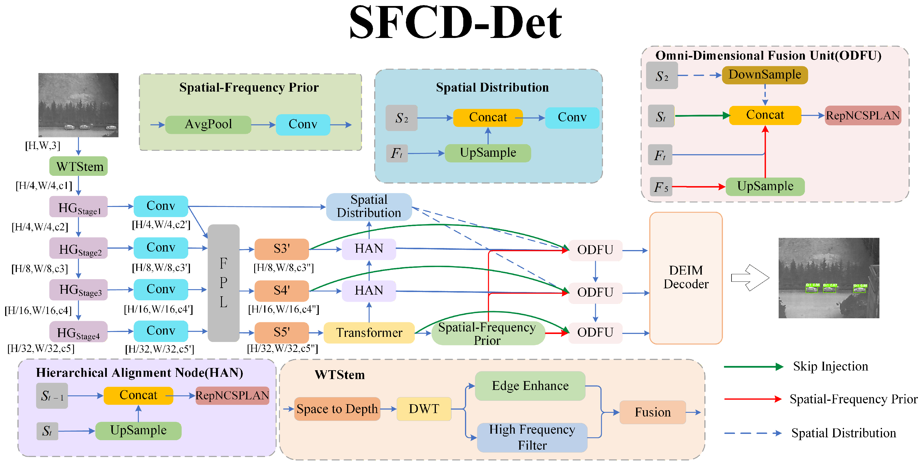
Figure 1.
Overall structure of SFCD-Det. The proposed detector introduces WTStem for early spatial–frequency feature preservation, FPL for adjacent-scale feature purification, and SFCFP for coordinated multi-scale reconstruction.
Figure 1.
Overall structure of SFCD-Det. The proposed detector introduces WTStem for early spatial–frequency feature preservation, FPL for adjacent-scale feature purification, and SFCFP for coordinated multi-scale reconstruction.
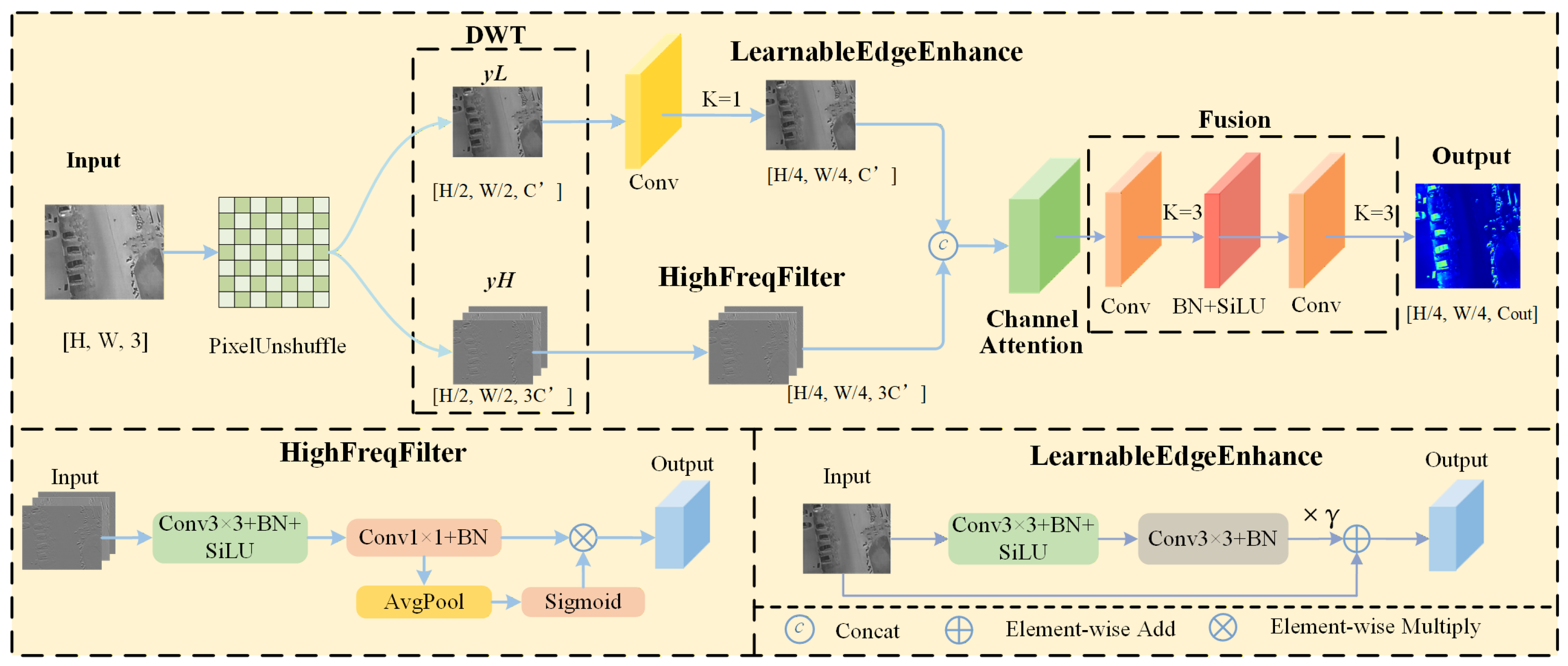
Figure 2.
Structure of the proposed WTStem. The input image is decoupled into orthogonal frequency sub-bands, followed by a dual-branch adaptive enhancement strategy for initial signal preservation.
Figure 2.
Structure of the proposed WTStem. The input image is decoupled into orthogonal frequency sub-bands, followed by a dual-branch adaptive enhancement strategy for initial signal preservation.
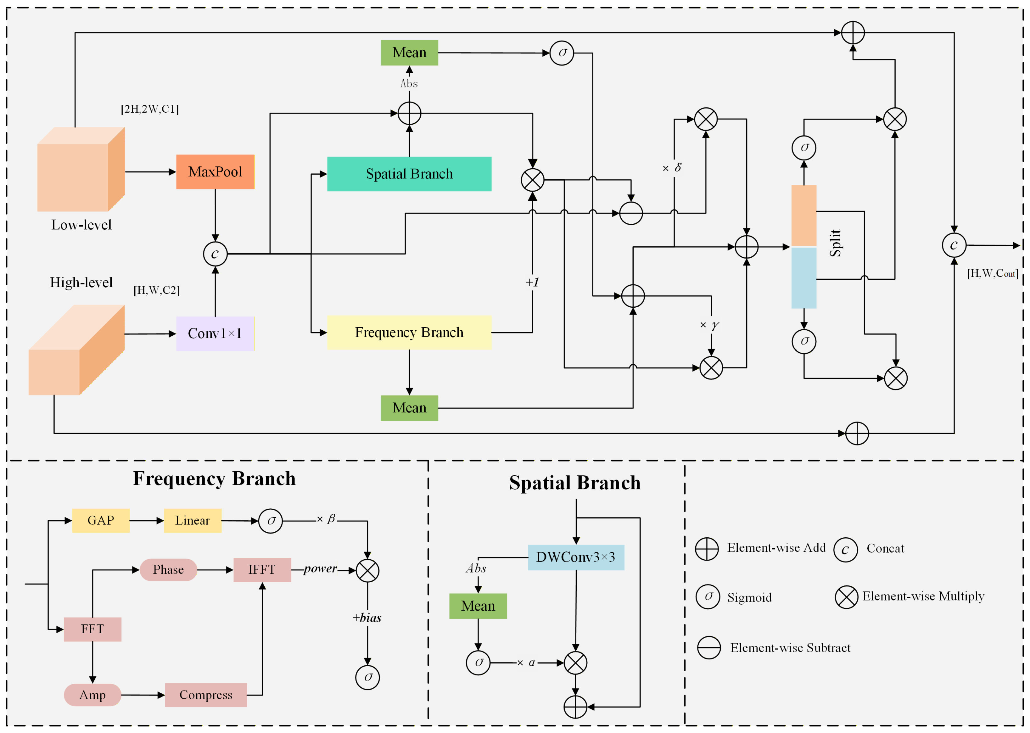
Figure 3.
Architecture of the FDAF module. FDAF models adjacent-scale feature interaction through spatial response encoding and spatial–frequency dynamic modulation.
Figure 3.
Architecture of the FDAF module. FDAF models adjacent-scale feature interaction through spatial response encoding and spatial–frequency dynamic modulation.
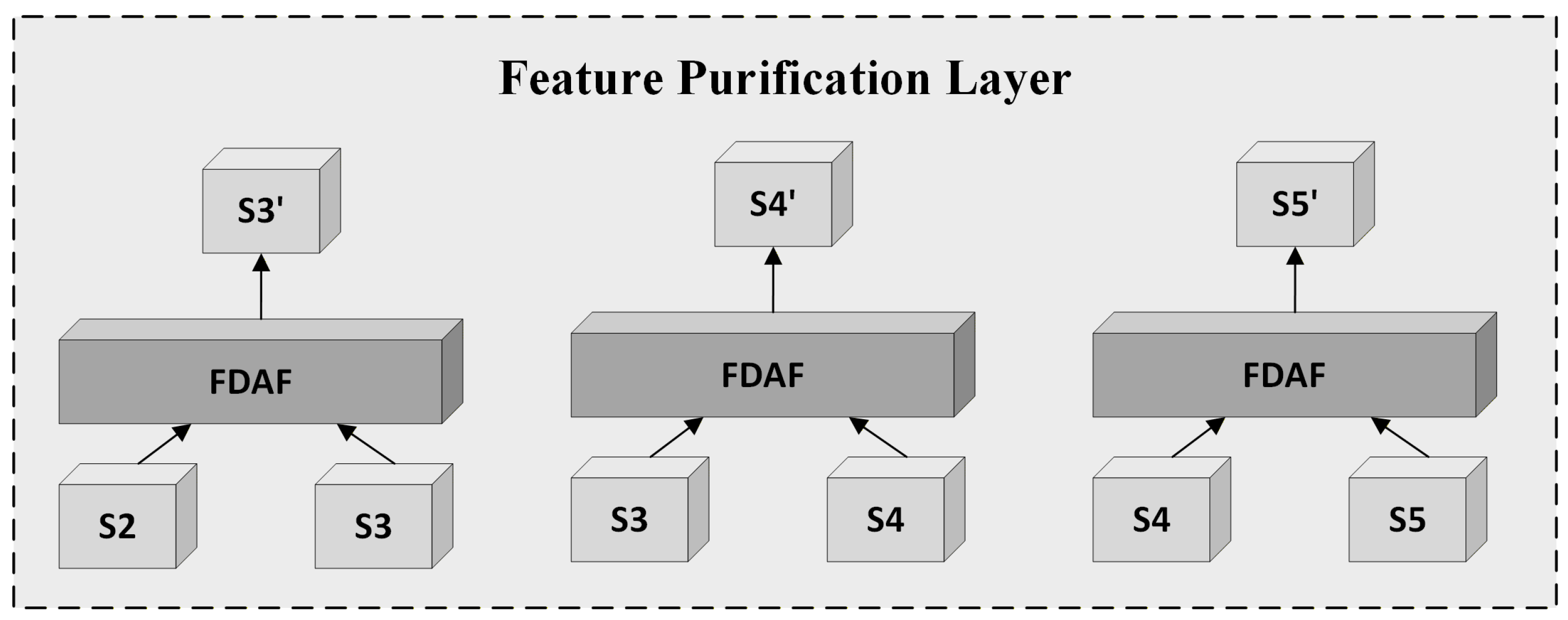
Figure 4.
Structure of the Feature Purification Layer (FPL). The layer integrates FDAF units to perform adjacent-scale feature purification.
Figure 4.
Structure of the Feature Purification Layer (FPL). The layer integrates FDAF units to perform adjacent-scale feature purification.
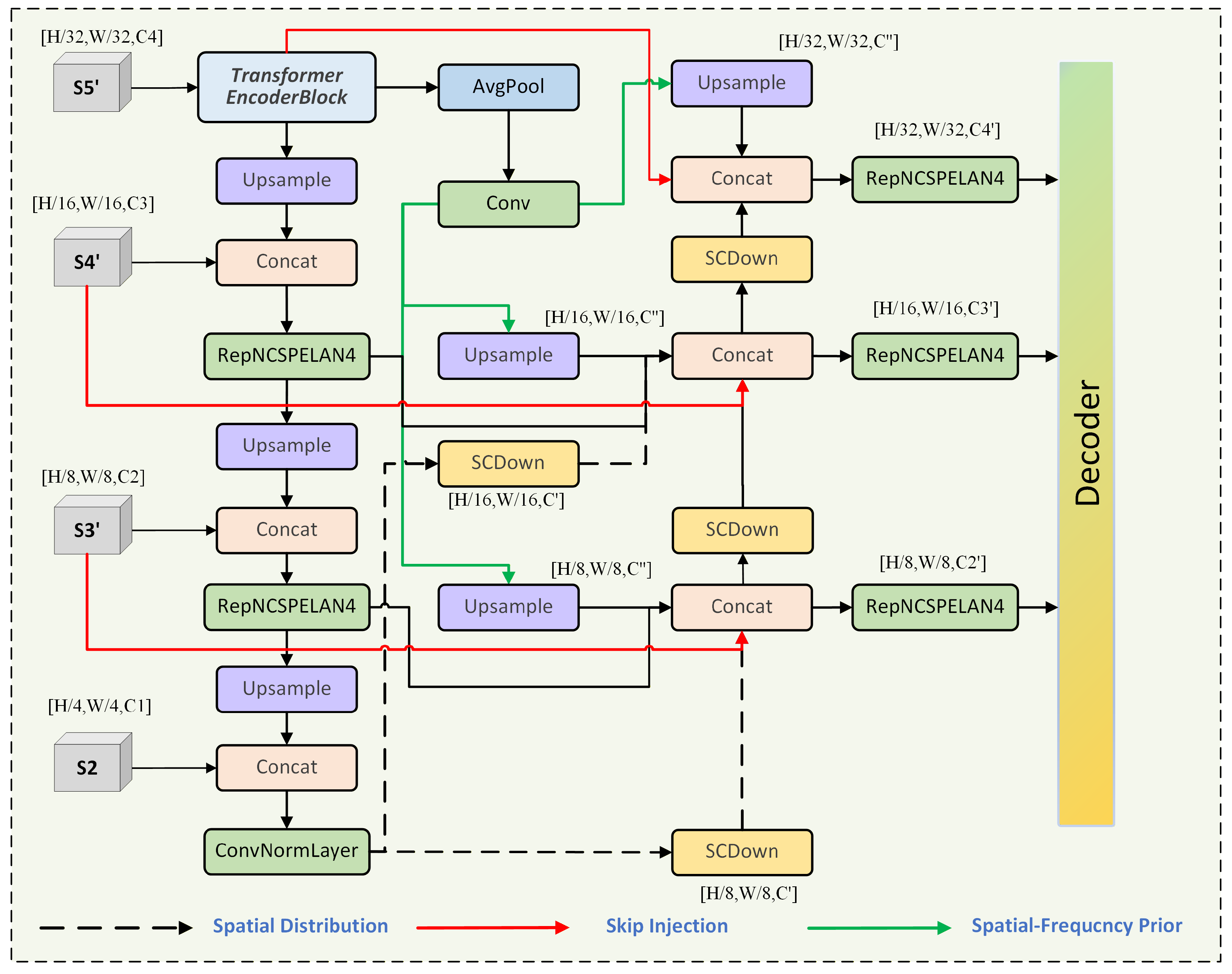
Figure 5.
Structure of the Spatial–Frequency Coordinated Feature Pyramid (SFCFP). SFCFP receives and the purified features , , and and reconstructs discriminative multi-scale features through S2 spatial distribution, S5 spatial–frequency prior broadcasting, and purified intermediate skip injection.
Figure 5.
Structure of the Spatial–Frequency Coordinated Feature Pyramid (SFCFP). SFCFP receives and the purified features , , and and reconstructs discriminative multi-scale features through S2 spatial distribution, S5 spatial–frequency prior broadcasting, and purified intermediate skip injection.
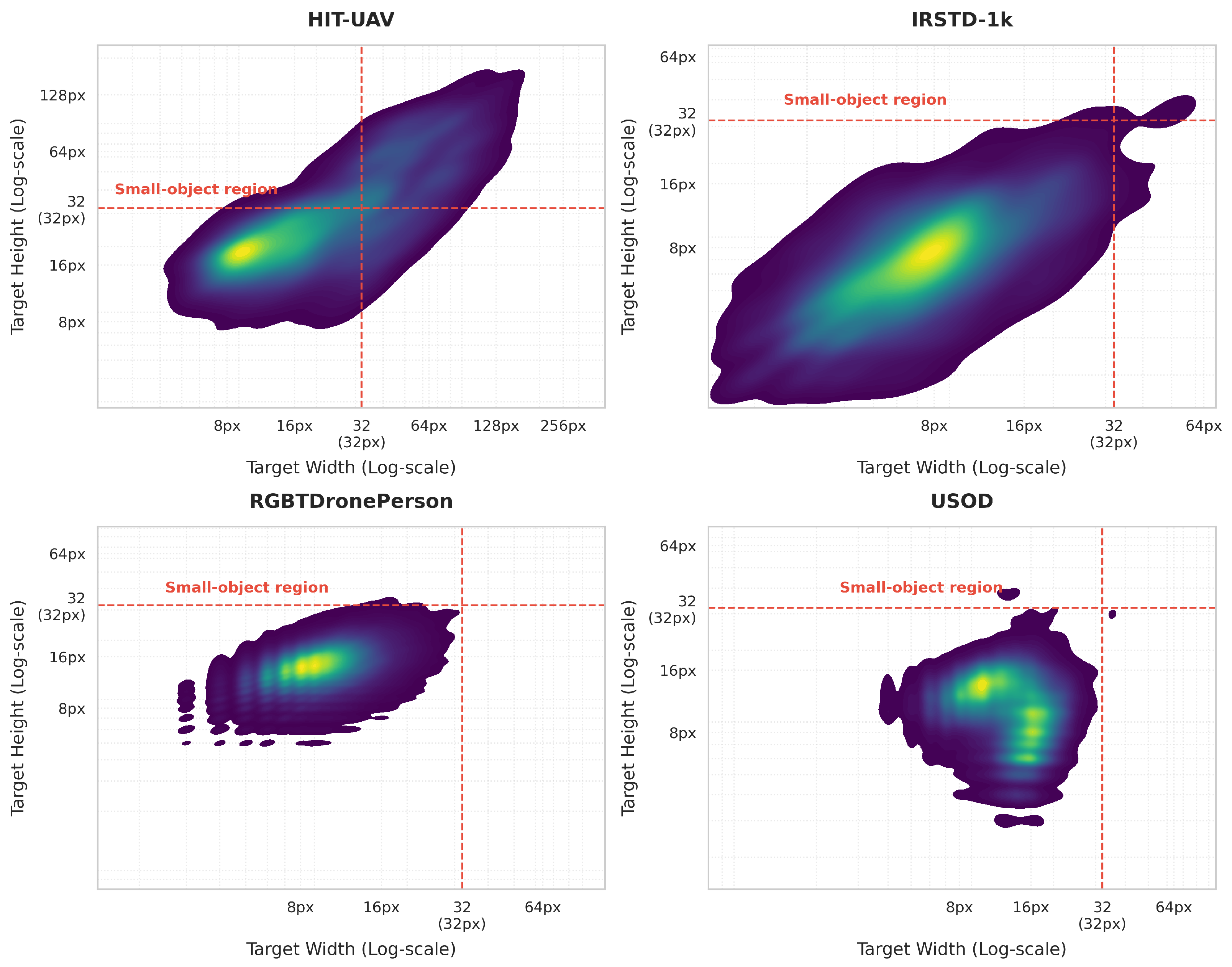
Figure 6.
Target width–height distributions of HIT-UAV, IRSTD-1K, RGBTDronePerson, and USOD in logarithmic coordinate space.
Figure 6.
Target width–height distributions of HIT-UAV, IRSTD-1K, RGBTDronePerson, and USOD in logarithmic coordinate space.
Figure 7.
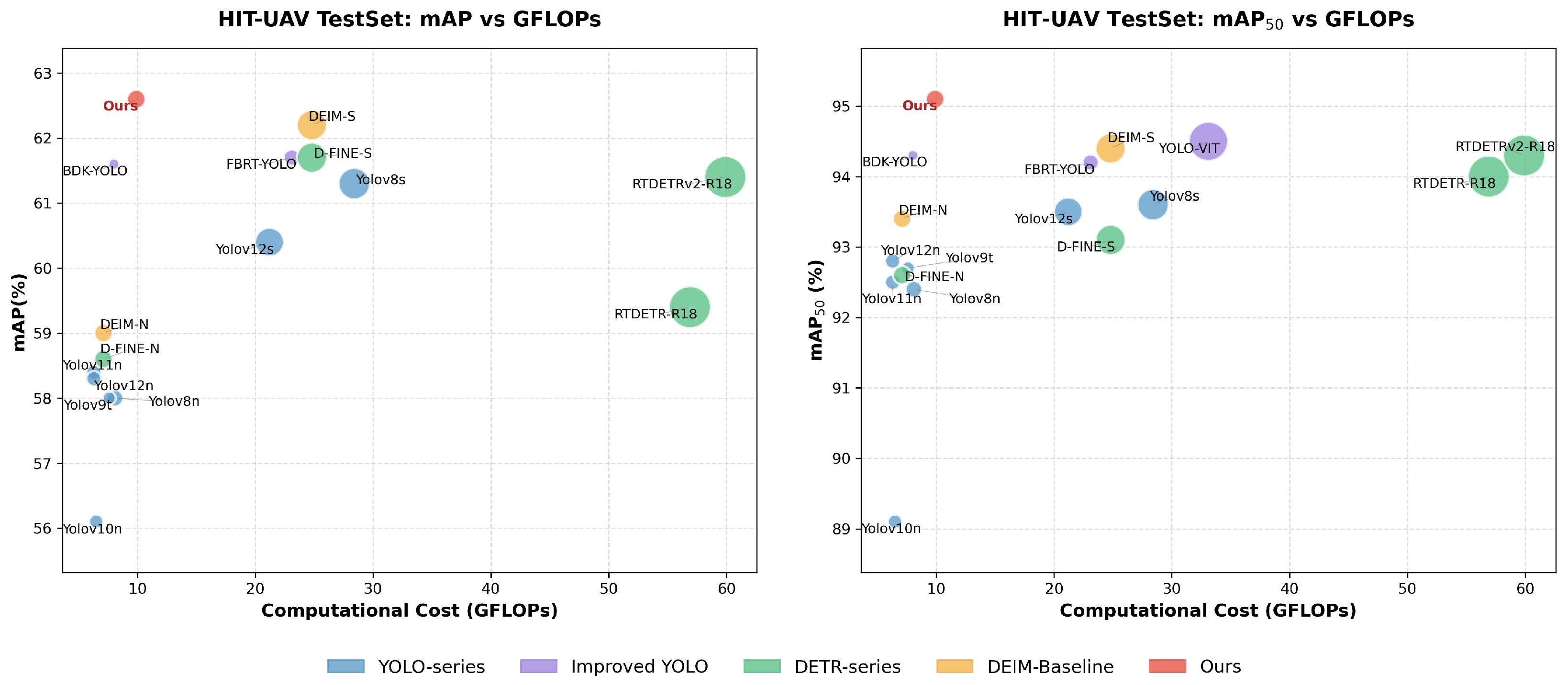
Accuracy vs. computational cost on the HIT-UAV test set. The bubble area indicates the parameter count. The top-left region indicates models with higher detection accuracy and lower reported parameter and FLOP costs.
Figure 7.
Accuracy vs. computational cost on the HIT-UAV test set. The bubble area indicates the parameter count. The top-left region indicates models with higher detection accuracy and lower reported parameter and FLOP costs.
Figure 8.
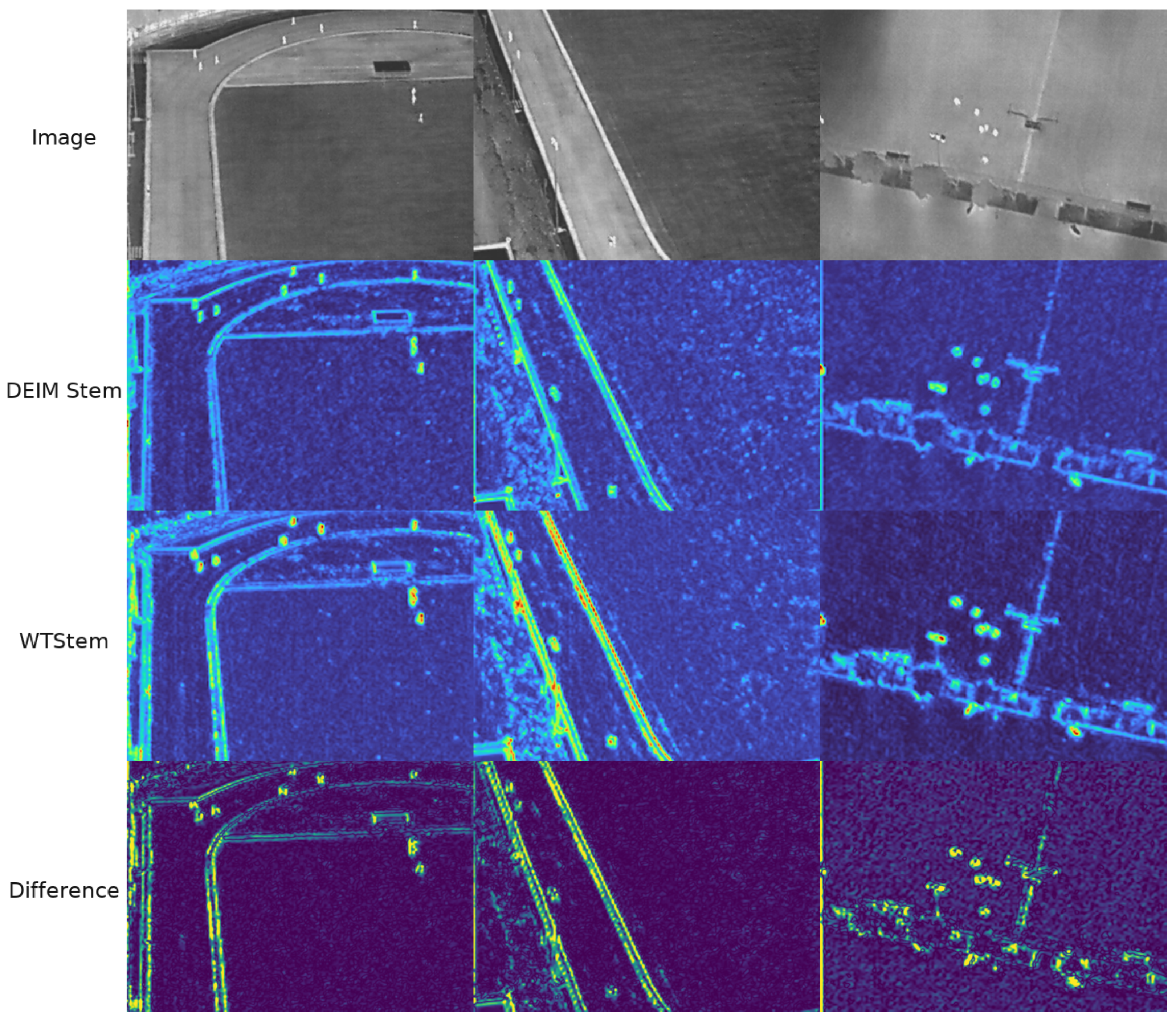
Visual comparison of initial signal preservation between the baseline stem and WTStem.
Figure 8.
Visual comparison of initial signal preservation between the baseline stem and WTStem.
Figure 9.
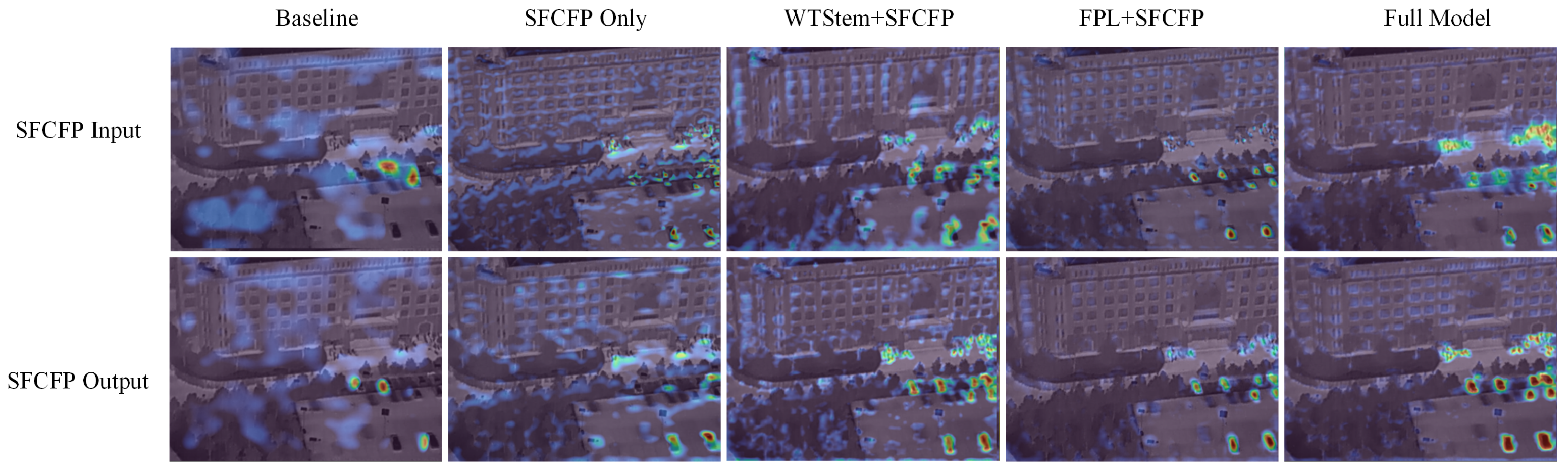
Visual comparison of SFCFP input and output activations under different module combinations.
Figure 9.
Visual comparison of SFCFP input and output activations under different module combinations.
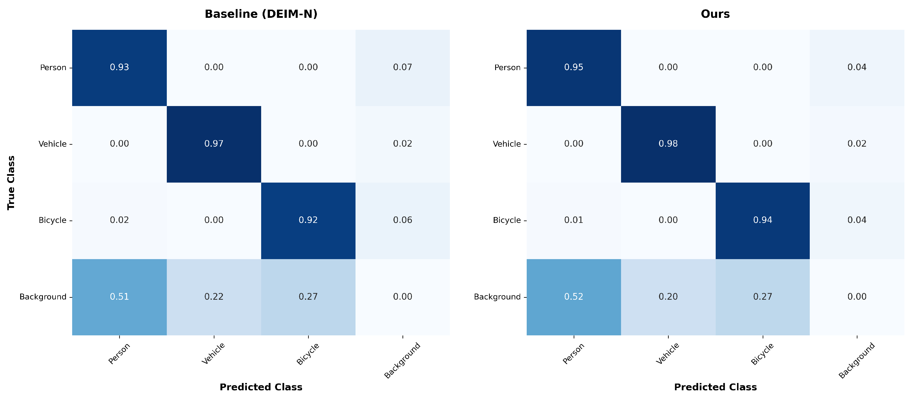
Figure 10.
Confusion matrix comparison between the baseline DEIM-N and our proposed method.
Figure 10.
Confusion matrix comparison between the baseline DEIM-N and our proposed method.
Figure 11.
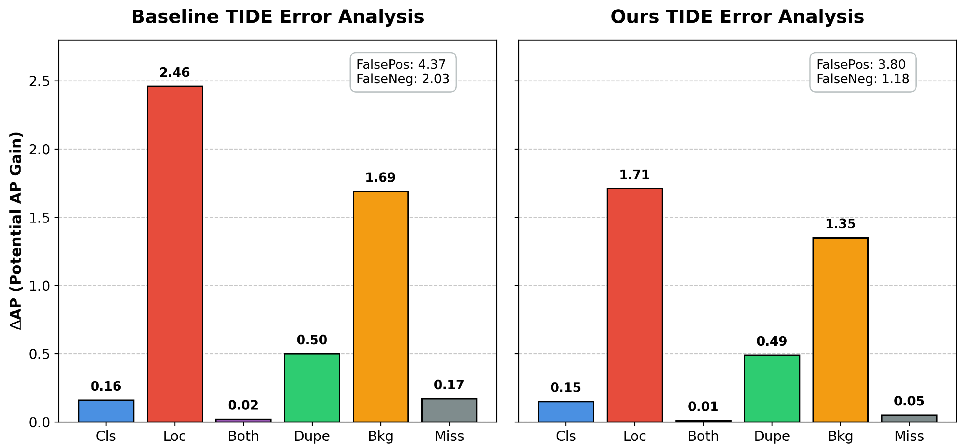
TIDE error analysis comparison between the baseline DEIM-N and our proposed method.
Figure 11.
TIDE error analysis comparison between the baseline DEIM-N and our proposed method.
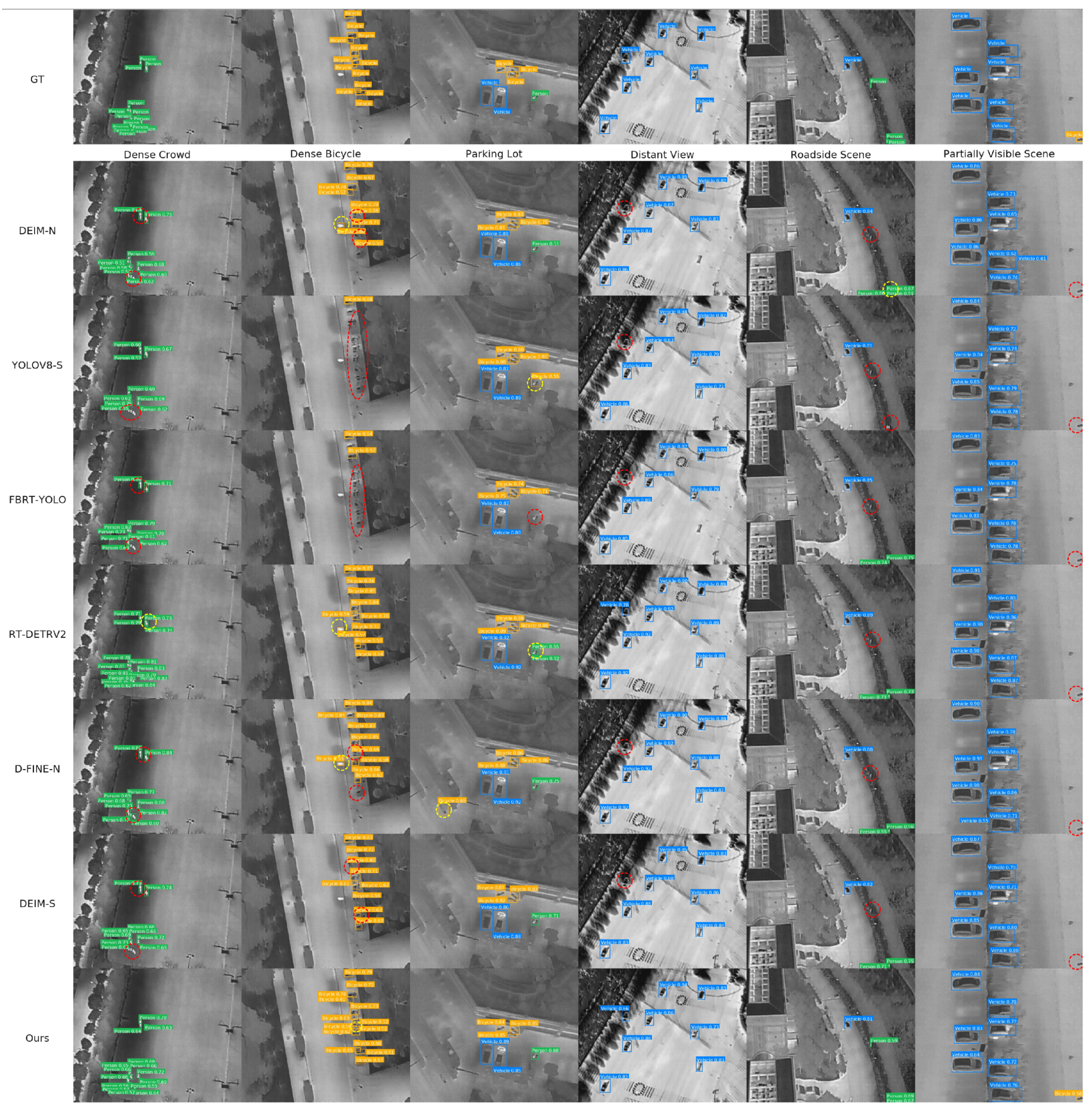
Figure 12.
Visual detection examples on HIT-UAV under typical UAV infrared scenarios. Red circles indicate visually identifiable missed detections, while yellow circles denote false predictions.
Figure 12.
Visual detection examples on HIT-UAV under typical UAV infrared scenarios. Red circles indicate visually identifiable missed detections, while yellow circles denote false predictions.
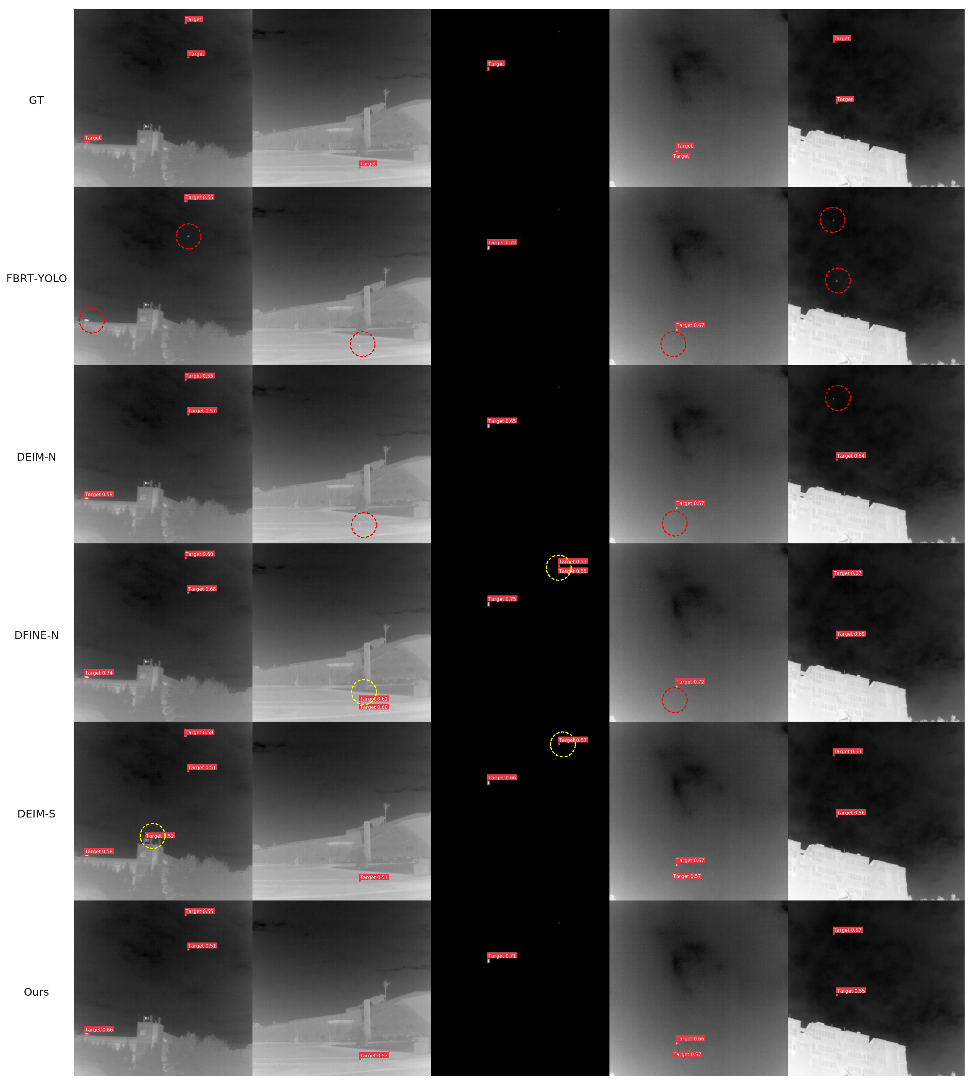
Figure 13.
Visual detection examples on IRSTD-1K under cluttered infrared backgrounds. Red circles indicate visually identifiable missed detections, yellow circles denote false predictions, and white circles indicate detected objects whose predicted bounding boxes do not fully cover the entire object.
Figure 13.
Visual detection examples on IRSTD-1K under cluttered infrared backgrounds. Red circles indicate visually identifiable missed detections, yellow circles denote false predictions, and white circles indicate detected objects whose predicted bounding boxes do not fully cover the entire object.
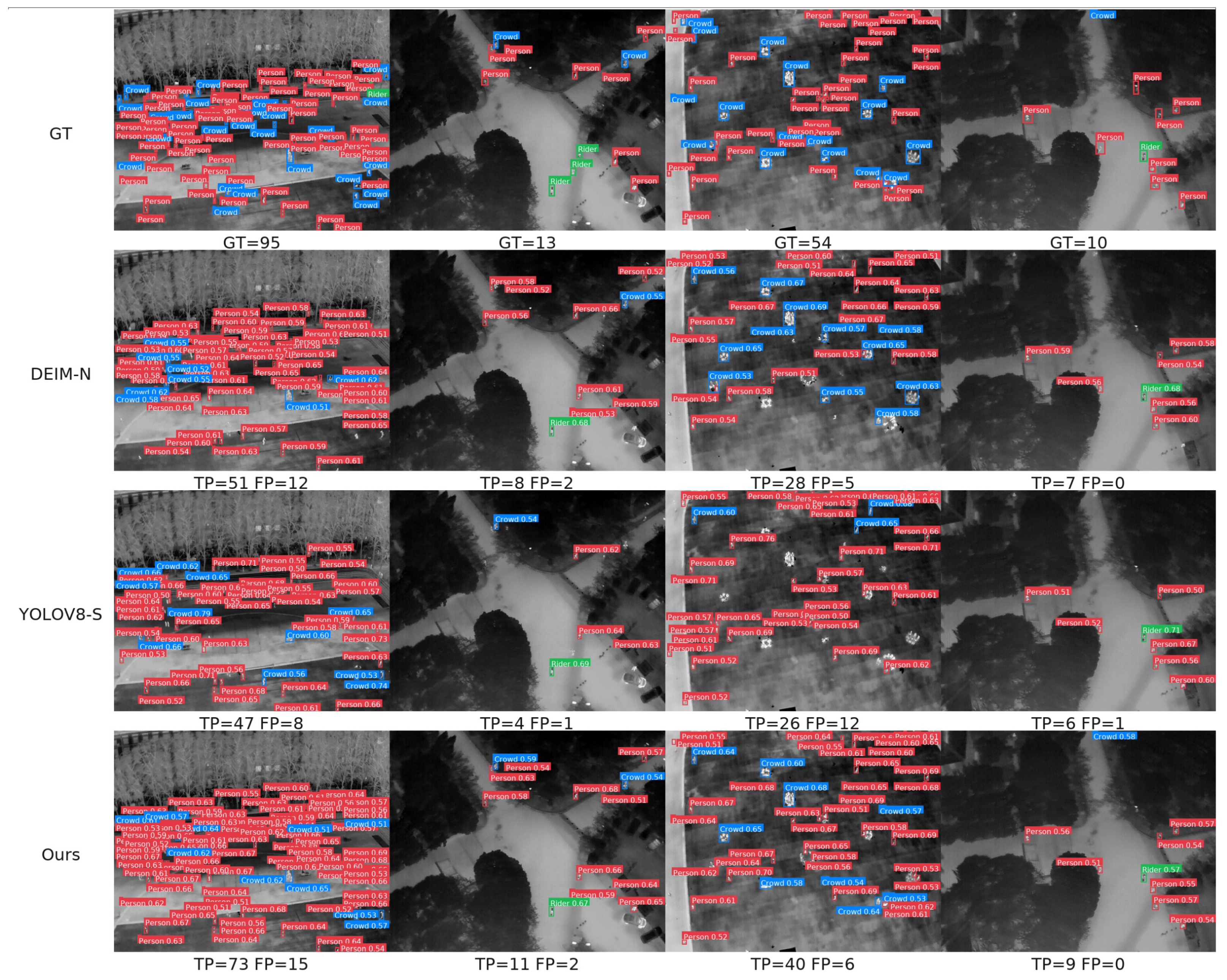
Figure 14.
Visual detection examples on the RGBTDronePerson dataset are provided to intuitively analyze model predictions in terms of TP and FP detection cases.
Figure 14.
Visual detection examples on the RGBTDronePerson dataset are provided to intuitively analyze model predictions in terms of TP and FP detection cases.
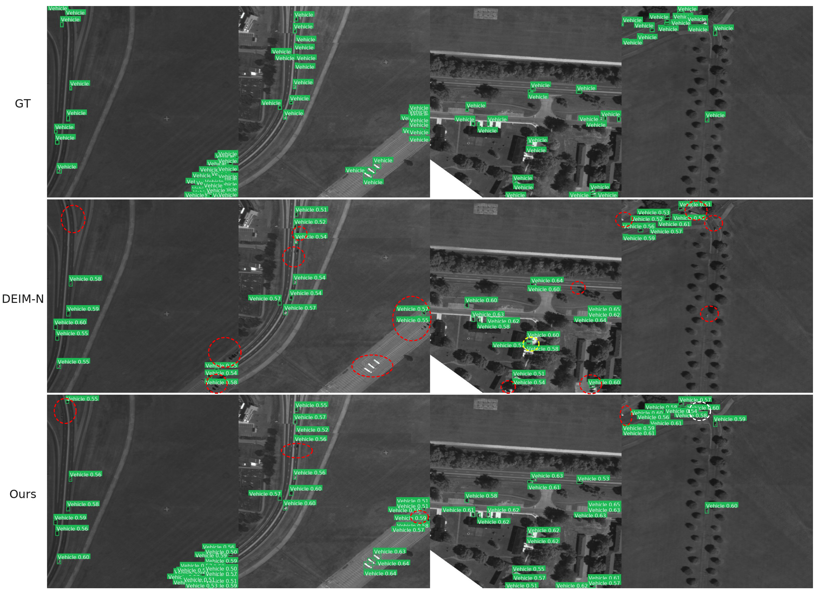
Figure 15.
Visual detection examples on USOD under low illumination and shadow occlusion. Red circles indicate visually identifiable missed detections, yellow circles denote false predictions, and white circles indicate detected objects whose predicted bounding boxes do not fully cover the entire object.
Figure 15.
Visual detection examples on USOD under low illumination and shadow occlusion. Red circles indicate visually identifiable missed detections, yellow circles denote false predictions, and white circles indicate detected objects whose predicted bounding boxes do not fully cover the entire object.
Table 1.
Implementation settings used for model training and evaluation.
Table 1.
Implementation settings used for model training and evaluation.
| Item | Setting |
|---|
| GPU | NVIDIA A100 |
| CPU | AMD EPYC 7742 64-Core Processor |
| Framework | PyTorch 2.3.0 |
| Python Version | Python 3.10 |
| Batch Size | 8 |
| Optimizer | AdamW |
| Initial Learning Rate | |
| Weight Decay | |
| Resize | |
Table 2.
Detection performance of advanced detectors on the HIT-UAV dataset. ‘Per.’, ‘Veh.’, and ‘Bic.’ denote the Person, Vehicle, and Bicycle categories. Bold and underline indicate the best and second-best results. The downward arrow indicates that lower values are better.
Table 2.
Detection performance of advanced detectors on the HIT-UAV dataset. ‘Per.’, ‘Veh.’, and ‘Bic.’ denote the Person, Vehicle, and Bicycle categories. Bold and underline indicate the best and second-best results. The downward arrow indicates that lower values are better.
| Method | Per. (%) | Veh. (%) | Bic. (%) | mAP (%) | mAP50 (%) | P (%) | R (%) | Params (M) ↓ | FLOPs (G) ↓ |
|---|
| YOLOv8-N | 91.0 | 97.5 | 88.6 | 58.0 | 92.4 | 90.4 | 87.1 | 3.01 | 8.1 |
| YOLOv8-S | 92.2 | 97.1 | 91.5 | 61.3 | 93.6 | 91.8 | 89.2 | 11.13 | 28.4 |
| YOLOv9-T | 90.4 | 97.5 | 90.1 | 58.0 | 92.7 | 89.6 | 88.0 | 1.97 | 7.6 |
| YOLOv10-N | 88.4 | 95.4 | 83.5 | 56.1 | 89.1 | 83.2 | 83.3 | 2.27 | 6.5 |
| YOLOv11-N | 91.3 | 97.7 | 88.6 | 58.4 | 92.5 | 89.9 | 86.9 | 2.58 | 6.3 |
| YOLOv12-N | 91.0 | 97.6 | 89.8 | 58.3 | 92.8 | 90.7 | 87.2 | 2.56 | 6.3 |
| YOLOv12-S | 92.5 | 96.4 | 91.5 | 60.4 | 93.5 | 92.0 | 88.3 | 9.23 | 21.2 |
| RT-DETR-R18 | 93.9 | 96.5 | 91.5 | 59.4 | 94.0 | 93.0 | 89.4 | 19.87 | 56.9 |
| RT-DETRv2-R18 | 93.7 | 97.6 | 91.7 | 61.4 | 94.3 | 90.5 | 89.5 | 19.88 | 59.9 |
| D-FINE-N | 91.6 | 96.5 | 89.6 | 58.6 | 92.6 | 89.4 | 87.1 | 3.72 | 7.1 |
| D-FINE-S | 93.1 | 97.0 | 89.3 | 61.7 | 93.1 | 90.3 | 87.1 | 10.18 | 24.8 |
| DEIM-N | 92.5 | 97.1 | 90.6 | 59.0 | 93.4 | 89.7 | 88.1 | 3.72 | 7.1 |
| DEIM-S | 93.9 | 97.0 | 92.4 | 62.2 | 94.4 | 91.0 | 90.2 | 10.18 | 24.8 |
| FBRT-YOLO | 92.4 | 97.8 | 92.5 | 61.7 | 94.2 | 91.6 | 90.0 | 2.90 | 23.1 |
| YOLO-VIT | 93.3 | 98.1 | 92.0 | - | 94.5 | 90.0 | 91.3 | 17.30 | 33.1 |
| BDK-YOLO | - | - | - | 61.6 | 94.3 | 90.5 | 90.3 | 1.35 | 8.0 |
| Ours | 94.7 | 97.8 | 92.7 | 62.6 | 95.1 | 91.2 | 90.9 | 3.81 | 9.9 |
Table 3.
Detection performance of advanced detectors on the IRSTD-1K dataset. Bold and underline indicate the best and second-best results. The downward arrow indicates that lower values are better.
Table 3.
Detection performance of advanced detectors on the IRSTD-1K dataset. Bold and underline indicate the best and second-best results. The downward arrow indicates that lower values are better.
| Method | mAP (%) | mAP50 (%) | P (%) | R (%) | Params (M) ↓ | FLOPs (G) ↓ |
|---|
| YOLOv8-N | 38.0 | 83.4 | 86.7 | 78.1 | 3.01 | 8.1 |
| YOLOv9-T | 35.2 | 80.5 | 85.0 | 77.9 | 1.97 | 7.6 |
| YOLOv11-N | 37.8 | 81.8 | 87.8 | 76.4 | 2.58 | 6.3 |
| YOLOv12-N | 37.2 | 82.3 | 84.7 | 80.8 | 2.56 | 6.3 |
| RT-DETR-R18 | 40.2 | 85.3 | 87.0 | 80.8 | 19.87 | 56.9 |
| D-FINE-N | 38.7 | 83.1 | 84.3 | 81.1 | 3.72 | 7.1 |
| D-FINE-S | 39.4 | 83.9 | 83.1 | 82.9 | 10.18 | 24.8 |
| DEIM-N | 39.0 | 83.7 | 83.4 | 82.7 | 3.72 | 7.1 |
| DEIM-S | 40.8 | 84.6 | 85.3 | 83.2 | 10.18 | 24.8 |
| FBRT-YOLO | 39.1 | 82.0 | 85.6 | 75.0 | 2.90 | 23.1 |
| IRMSD-YOLO | 41.2 | 86.2 | 89.1 | 83.1 | 8.35 | 37.1 |
| Ours | 41.4 | 86.4 | 83.5 | 85.0 | 3.81 | 9.9 |
Table 4.
Detection performance of advanced detectors on the RGBTDronePerson dataset. Bold and underline indicate the best and second-best results. The downward arrow indicates that lower values are better.
Table 4.
Detection performance of advanced detectors on the RGBTDronePerson dataset. Bold and underline indicate the best and second-best results. The downward arrow indicates that lower values are better.
| Method | mAP (%) | mAP50 (%) | P (%) | R (%) | Params (M) ↓ | FLOPs (G) ↓ |
|---|
| YOLOv8-S | 13.0 | 37.9 | 48.7 | 45.5 | 11.13 | 28.4 |
| YOLOv11-S | 14.3 | 40.8 | 52.3 | 44.9 | 9.41 | 21.3 |
| YOLOv12-M | 15.6 | 43.1 | 51.9 | 45.5 | 20.1 | 67.1 |
| FBRT-YOLO | 13.0 | 35.5 | 44.7 | 40.6 | 2.90 | 23.1 |
| D-FINE-S | 16.5 | 45.8 | 50.7 | 52.9 | 10.18 | 24.8 |
| DEIM-N | 15.8 | 44.3 | 50.8 | 49.5 | 3.72 | 7.1 |
| Ours | 16.8 | 46.8 | 53.2 | 53.6 | 3.81 | 9.9 |
Table 5.
Detection performance of advanced detectors on the USOD dataset. Bold and underline indicate the best and second-best results. The downward arrow indicates that lower values are better.
Table 5.
Detection performance of advanced detectors on the USOD dataset. Bold and underline indicate the best and second-best results. The downward arrow indicates that lower values are better.
| Method | mAP (%) | mAP50 (%) | P (%) | R (%) | Params (M) ↓ | FLOPs (G) ↓ |
|---|
| YOLOv8-S | 30.1 | 85.1 | 87.3 | 81.5 | 11.13 | 28.4 |
| YOLOv11-S | 32.3 | 87.5 | 89.4 | 82.5 | 9.41 | 21.3 |
| FBRT-YOLO | 28.3 | 83.1 | 85.5 | 80.4 | 2.90 | 23.1 |
| DEIM-N | 32.7 | 85.1 | 85.8 | 78.1 | 3.72 | 7.1 |
| Ours | 34.1 | 88.0 | 87.8 | 81.7 | 3.81 | 9.9 |
Table 6.
Ablation study of the proposed components on the HIT-UAV dataset.
Table 6.
Ablation study of the proposed components on the HIT-UAV dataset.
| Variant | WTStem | FPL | SFCFP | mAP (%) | mAP50 (%) | P (%) | R (%) |
|---|
| Baseline | - | - | - | 59.0 | 93.4 | 89.7 | 88.1 |
| Exp. 1 | ✔ | - | - | 59.8 | 93.9 | 90.1 | 89.6 |
| Exp. 2 | - | ✔ | - | 60.1 | 94.1 | 90.6 | 89.4 |
| Exp. 3 | - | - | ✔ | 61.2 | 93.8 | 90.0 | 89.1 |
| Exp. 4 | ✔ | - | ✔ | 61.8 | 94.3 | 91.1 | 90.0 |
| Exp. 5 | - | ✔ | ✔ | 62.0 | 94.6 | 90.3 | 90.4 |
| Exp. 6 | ✔ | ✔ | ✔ | 62.6 | 95.1 | 91.2 | 90.9 |
Table 7.
Accuracy and computational cost of different stem designs. Bold and underline indicate the best and second-best results. The downward arrow indicates that lower values are better.
Table 7.
Accuracy and computational cost of different stem designs. Bold and underline indicate the best and second-best results. The downward arrow indicates that lower values are better.
| Method | mAP (%) | mAP50 (%) | P (%) | R (%) | Params (M) ↓ | FLOPs (G) ↓ |
|---|
| DEIM-N | 59.0 | 93.4 | 89.7 | 88.1 | 3.72 | 7.1 |
| SRFD | 59.4 | 93.8 | 90.3 | 89.2 | 3.72 | 7.3 |
| LOGStem | 59.4 | 93.5 | 89.8 | 89.1 | 3.76 | 15.4 |
| RepStem | 58.5 | 93.2 | 89.7 | 88.6 | 3.72 | 6.7 |
| WTStem | 59.8 | 93.9 | 90.1 | 89.6 | 3.74 | 7.5 |
Table 8.
Accuracy and computational cost of different feature pyramid network designs. Bold and underline indicate the best and second-best results. The downward arrow indicates that lower values are better.
Table 8.
Accuracy and computational cost of different feature pyramid network designs. Bold and underline indicate the best and second-best results. The downward arrow indicates that lower values are better.
| Method | mAP (%) | mAP50 (%) | P (%) | R (%) | Params (M) ↓ | FLOPs (G) ↓ |
|---|
| DEIM-N | 59.0 | 93.4 | 89.7 | 88.1 | 3.72 | 7.1 |
| HS-FPN | 59.9 | 93.2 | 88.9 | 88.6 | 5.36 | 10.7 |
| GoldYOLO | 59.8 | 93.8 | 90.0 | 89.1 | 4.17 | 7.2 |
| HyperACE | 59.3 | 93.4 | 89.9 | 88.5 | 4.08 | 8.1 |
| A3FPN | 59.2 | 93.1 | 90.5 | 88.7 | 3.73 | 7.1 |
| SFCFP | 61.2 | 93.8 | 90.0 | 89.1 | 3.60 | 9.3 |
Table 9.
Internal ablation study of different pathways in SFCFP on the HIT-UAV dataset.
Table 9.
Internal ablation study of different pathways in SFCFP on the HIT-UAV dataset.
| Method | S2 Path | S5 Prior | Skip Injection | mAP (%) | mA50 (%) | P (%) | R (%) |
|---|
| DEIM-N | - | - | - | 59.0 | 93.4 | 89.7 | 88.1 |
| SFCFP w/S2 | ✔ | - | - | 60.1 | 93.6 | 89.5 | 88.6 |
| SFCFP w/S2+S5 | ✔ | ✔ | - | 60.8 | 93.8 | 89.8 | 88.9 |
| Full SFCFP | ✔ | ✔ | ✔ | 61.2 | 93.8 | 90.0 | 89.1 |
Table 10.
Five-seed stability analysis, reported as mean ± standard deviation.
Table 10.
Five-seed stability analysis, reported as mean ± standard deviation.
| Dataset | Method | mAP (%) | mAP50 (%) | P (%) | R (%) |
|---|
| HIT-UAV | DEIM-S | | | | |
| HIT-UAV | SFCD-Det | | | | |
| RGBTDronePerson | D-FINE-S | | | | |
| RGBTDronePerson | SFCD-Det | | | | |