Practical Near-Field Illuminance Simulation for Visual Inspection Using Novel Method

Abstract

Near-field direct illumination from extended luminaires presents a fundamental modeling challenge in automated visual inspection: standard far-field IES (Illuminating Engineering Society) photometric data treat luminaires as point sources, an assumption that breaks down when source-to-target distances are comparable to luminaire dimensions. This paper addresses this breakdown by establishing, both analytically and experimentally, the conditions under which IES-based point-source discretization remains valid and the minimum discretization required when it does not. A solid-angle-based illuminance formulation on triangular meshes is coupled with a controlled virtual-emitter discretization of elongated luminaires, and a reproducible selection workflow is derived that relates emitter count to the source–target distance ratio and a specified error criterion. The dependence of discretization requirements on source–target distance is characterized by an angular-subtense argument, yielding the scaling relation $N\sim (L/H)·C$, where L is the luminaire length, H the working distance, and C a constant determined by the IES angular gradient and the required accuracy. Validation experiments with one and two industrial linear luminaires (1.2 m, Banner Engineering WLS15xDW1200Dx) include single-luminaire heights of $H=20\mathrm{cm}$, $25\mathrm{cm}$, $35\mathrm{cm}$, $50\mathrm{cm}$, and $60\mathrm{cm}$, as well as effective-length reduction cases produced by opaque end masking at $H=35\mathrm{cm}$. The single-luminaire validation set compares $N=1$–7 virtual emitters for all cases, with the $H=20\mathrm{cm}$ case extended to $N=9$. The selected emitter counts are chosen as the best-performing candidate simulations after considering scalar error, smoothness, and profile consistency. The selected uncovered cases are $N=9$ at $H=20\mathrm{cm}$, $N=7$ at $H=25\mathrm{cm}$, $N=5$ at $H=35\mathrm{cm}$, and $N=3$ at $H=50$–$60\mathrm{cm}$. The masked-source experiments confirm that reducing the effective source length at fixed height reduces the required emitter count. The fitted selection relation developed from these cases indicates that the working distance H has the stronger influence within the tested range. The method provides a computationally efficient, practitioner-ready tool for inspection-lighting design when near-field goniophotometry or optical ray tracing is unavailable.

1. Introduction

Visual inspection is a cornerstone of modern industrial and manufacturing processes, particularly in smart factories and in-line quality assurance. Well-designed illumination is critical for repeatability, defect detectability, and measurement stability, and it also informs inspection cell design including sensor placement, fixturing, and shielding. As source-to-target distances in conveyor-based and robot-arm inspection systems are often in the order of the luminaire dimensions, near-field illumination modeling is an essential but underserved component of inspection system design.

In this work, near field and far field are used primarily in a geometric and photometric sense. In classical luminaire photometry, the far-field condition is reached when the source–detector distance is sufficiently large that the finite luminous extent of the luminaire no longer produces a significant distance-dependent change in the measured angular luminous-intensity distribution. Under this condition, the luminaire can be represented by a photometric center, and the inverse-square-law point-source model can be applied within the required measurement uncertainty [1,2,3]. The near field refers to shorter distances for which different parts of an extended source subtend appreciably different directions and solid angles at the receiver, so the spatial origin of the emitted light remains important [4,5]. Consequently, there is no single universal geometric ratio that defines the transition for every luminaire; the applicable photometric distance depends on source dimensions, optical construction, beam shape, detector geometry, and the required uncertainty. Visual inspection refers specifically to machine-vision-based inspection systems used in industrial automation, where cameras and illumination are deployed to detect defects, measure geometry, or assess surface quality.

Illumination design has received sustained attention in the inspection literature because variations in lighting conditions can affect the performance of trained AI-based vision models when they are deployed in environments that differ from those used during training. For example, machine-vision methods have been applied to autonomous steel-pipe weld-line inspection, where consistent illumination can play an important role in maintaining reliable image-based defect detection [6]. Structured lighting enhances defect detectability on specular surfaces by controlling illumination geometry and reflection paths [7]. Adaptive illumination strategies have been proposed for complex industrial parts where spatial light distribution dominates inspection performance [8]. Specialized setups such as annular and coaxial sources improve performance on low-contrast weld lines [9], and multi-light-source acquisition enables feature extraction under varying directions on highly reflective surfaces [10]. Camera deployment methods have been developed for triangular-facet inspection [11] and extended to continuous pose sets for machine-vision systems [12]. Collectively, this literature underscores the centrality of illumination design but does not provide a general, efficient method for near-field light modeling from standardized photometric data.

Recent reviews of manufacturing computer vision further identify lighting as a core component of industrial vision systems rather than an auxiliary detail. Zhou et al. [13] reviewed computer-vision applications across manufacturing and included the lighting module as part of the manufacturing-oriented vision-system framework. Ren et al. [14] emphasized that high-quality optical illumination and suitable image acquisition hardware are prerequisites for reliable defect detection. Kim et al. [15] similarly identified the light source as one of the principal components of a machine-vision system and discussed automated inspection and quality control as major application areas. These studies motivate the present focus on illumination modeling for compact visual-inspection cells.

Several factors contribute to the scarcity of general near-field visual-detection research based on standardized photometric data. First, manufacturer IES files normally provide whole-luminaire far-field luminous-intensity distributions rather than spatially resolved near-field source information. Second, detailed optical geometry, diffuser properties, LED pitch, package-level output variation, and material data are often proprietary or unavailable to inspection engineers. Third, near-field goniophotometric measurements require specialized equipment and are rarely supplied for industrial machine-vision luminaires. Finally, inspection performance is highly application-specific: the useful illumination field depends on target reflectance, defect type, camera pose, working distance, shielding, and fixture constraints. These factors make it difficult to build a universal near-field model directly from standardized photometric files and motivate a practical validation workflow that can be repeated for a given luminaire and inspection geometry.

On the modeling side, IES photometric files encode far-field luminous intensity distributions in a standardized format [16] and are the most universally available photometric description for industrial luminaires. The solid-angle method is widely used to improve light-simulation accuracy [17]. However, the point-source assumption embedded in IES data breaks down in near-field conditions. Spatial simulation approaches for extended linear sources have demonstrated that inverse-square and point-source models fail at short distances [18]. Detailed near-field LED modeling via Monte Carlo ray tracing captures spatial photon distributions with high fidelity [19] but requires luminaire-specific geometric or chip-scale models and substantial computational cost. Prior work and standards explicitly motivate near-field goniophotometry or alternative formulations for extended sources [4,5]. Related studies have optimized illumination for surface-defect inspection [20,21], used structured or multi-source illumination to improve visual contrast [22,23], and investigated near-field behavior of extended LED sources through explicit spatial or optical models [5,24].

Despite this body of work, a fundamental question remains unanswered in the open literature: given only a standard manufacturer-provided IES file for an extended industrial luminaire, what is the minimum number of discrete virtual emitters required to reproduce near-field illuminance distributions within a specified error bound, and how does this requirement scale with the ratio of working distance to luminaire length? Prior work has addressed near-field behavior through Monte Carlo ray tracing or explicit LED-chip modeling, both of which require luminaire-specific geometric data that are unavailable in practice. Classical analytic formulations assume Lambertian or otherwise idealized emitters. No published methodology provides a reproducible, measurement-validated workflow for answering this question using only the photometric data format universally available from manufacturers. This paper fills that gap.

The proposed methodology couples standard IES intensity data with per-triangle solid-angle-based illuminance evaluation on mesh elements, augmented for elongated sources by a small set of virtual point emitters. This study emphasizes the method of selecting the emitter count for a given luminaire, working distance, and error criterion, rather than claiming a universal number. Validation uses one and two industrial-grade luminaires across multiple mounting heights, effective source-length cases created with opaque tape, and multi-source orientations, with each scenario repeated three times. The approach is limited to direct illumination; occluders and interreflections are not modeled. These choices align with applications where fast, near-field, direct-light estimation supports rapid iteration on fixture design, shielding, and sensor placement.

The method is intended for rapid engineering planning of visual-inspection cells, rather than for optical design of LED packages, lenses, reflectors, or diffusers. In practice, inspection engineers frequently have only the luminaire dimensions and a manufacturer IES file while needing to choose the mounting height, source placement, source number, and expected target coverage. The proposed workflow provides a low-data method for determining whether a single point-source IES model is sufficient and, when it is not, how many virtual emitters are required to reproduce the measured near-field illuminance distribution within the selected error and smoothness criteria.

2. Light Calculation

2.1. IES Models and Their Near-Field Limitations

Classical luminaire goniophotometry measures the directional luminous-intensity distribution of a test source in a defined angular coordinate system. The relevant measurement principles, coordinate systems, goniophotometer configurations, test conditions, and error sources are treated in CIE 070, CIE 121, and ANSI/IES LM-75 [1,2,3]. The measured distribution is commonly transferred in an IES photometric file as discrete values of luminous intensity versus angular direction [16]. Such a file is compact because it represents the luminaire through a photometric center and an angular intensity distribution rather than retaining the spatial origin of light over the emitting aperture.

A key concept in this measurement framework is the photometric test distance, i.e., the source–detector separation used when the angular luminous-intensity data are measured. For a far-field luminous-intensity description to be applicable, that distance must be sufficiently large that the finite dimensions of the test luminaire do not cause material distance-dependent changes in the measured distribution, and that the inverse-square relation between illuminance and distance is valid within the required measurement uncertainty [1,2]. Equivalently, if illuminance E is measured along a fixed direction at distance r, the derived quantity $I=E{r}^2$ should be effectively independent of r once the far-field condition has been reached. The required separation is therefore not a universal fixed multiple of luminaire size: it can depend on the maximum luminous dimension, beam narrowness or asymmetry, optical elements, detector aperture and field of view, alignment, and the uncertainty target of the test. This is why photometric distance is a central issue in classical luminaire photometry and why a laboratory far-field measurement distance should not be confused with the much shorter application working distance in a compact inspection cell.

Standard measurement documents such as ANSI/IES LM-79-19 and CIE S 025/E:2015 define controlled conditions for the photometric characterization of solid-state lighting products, while CIE 121 and ANSI/IES LM-75 provide broader guidance on luminaire photometry and goniophotometric measurement practice [2,3,25,26]. When the receiver is brought into the geometric near field of an extended luminaire, different source regions are viewed under different directions and distances, and a single photometric center can no longer reproduce the spatially varying illuminance accurately. Near-field goniophotometry addresses this problem by preserving spatial as well as angular information about the emitted light, allowing near-field quantities to be reconstructed without relying on a single point-source representation [4,5]. However, such data are substantially less available than standard manufacturer IES files.

The distinction is directly relevant to the present work. The manufacturer IES file is used here only as the available far-field angular descriptor of the complete luminaire; it is not assumed to contain a spatially resolved near-field source model. The application working distances considered in the experiments are comparable to, or smaller than, the $1.2\mathrm{m}$ luminaire length. Therefore, direct use of one whole-luminaire IES point source is expected to be inadequate because the IES file is a far-field angular representation rather than a spatially resolved near-field source map. The proposed method addresses this gap by redistributing the whole-luminaire IES intensity over a controlled set of virtual emitters and selecting the discretization experimentally for the application geometry.

Although machine vision ultimately depends on radiometric quantities at the image sensor, this work employs photometric quantities (illuminance) as engineering proxies for illumination coverage and uniformity during inspection-cell design. The method does not model spectral radiance, camera spectral response, lens vignetting, or image formation. It targets rapid planning and comparative evaluation of illumination configurations using manufacturer-provided photometric data.

Industrial inspection luminaires, particularly LED retrofits of linear form factors, consist of discrete emitters, optical diffusers, and internal structures whose effective emission characteristics are provided only through manufacturer-supplied IES files. Closed-form analytic expressions for illuminance from idealized Lambertian sources, while well documented in photometry handbooks, require a known luminance distribution that is not available in practice. The proposed method provides a pragmatic bridge between standardized far-field photometric data and near-field engineering needs.

2.2. Algorithmic Workflow

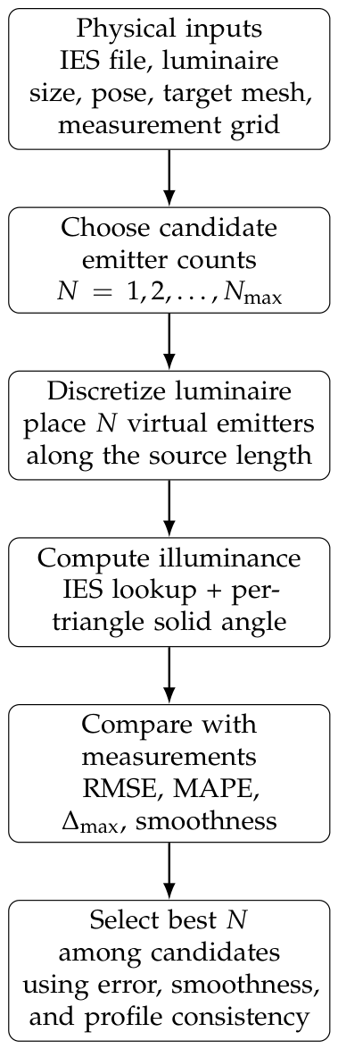
The complete workflow is summarized in Figure 1. It explicitly separates physical input data, numerical discretization of the extended luminaire, the solid-angle-based illuminance calculation, and the validation step used to select the selected number of virtual emitters.

• Geometry and Frames: Define the luminaire frame and target mesh frame; express source position and orientation in the target frame.
• IES Parsing and Interpolation: Read $I(\theta ,\varphi )$ from the IES file; evaluate I at required directions using bilinear interpolation.
• Candidate Emitter-Count Sweep: Select candidate virtual-emitter counts N, applied to the same luminaire at different working distances to isolate near-field geometry effects.
• Emitter Discretization: Approximate the extended luminaire using N equally spaced discrete emitters along its physical length, each assigned an equal luminous-flux share.
• Per-Element Evaluation: For each target mesh element, compute the direction vector from each emitter to the element centroid, evaluate $I(\theta ,\varphi )$, compute the element solid angle, and obtain the illuminance contribution.
• Aggregation: Sum contributions from all emitters to obtain the total illuminance field.
• Validation and Selection of N: Compare simulated and measured illuminance using RMSE, MAPE, maximum absolute deviation, the smoothness metric, and the stability of the central spatial profile. Select the candidate N that provides the best overall agreement and profile consistency among the simulated cases.

All computations use direct illumination only (no occlusion or interreflections). The workflow is intentionally modular: if detailed near-field goniophotometry, measured emitter non-uniformity, or diffuser properties become available, these data can replace the equal-emitter assumption without changing the solid-angle evaluation framework.

The simulator was implemented in Python 3.11 as a direct-illumination calculation. For each candidate value of N, the luminaire length is divided into N equally spaced virtual emitters. The IES file is treated as the far-field intensity distribution of the complete luminaire; therefore, the intensity contribution assigned to each virtual emitter is normalized by $1/N$. Each emitter uses the same angular shape from the IES file, but with one Nth of the whole-luminaire luminous-intensity magnitude. For each triangular mesh element, the direction from the emitter to the element centroid is used to interpolate the normalized luminous intensity from the IES table, the triangle solid angle is evaluated analytically, and the resulting luminous-flux contribution is divided by the element area to obtain illuminance. Contributions from all emitters are then summed. This normalization was used in all simulations and prevents the total predicted flux from increasing artificially with the number of virtual emitters.

Increasing N reduces discretization error and makes the model approach a continuous line-source approximation under the equal-emitter and identical-IES assumptions. In practice, the benefit saturates because a whole-luminaire IES file does not contain near-field source-level information such as individual LED locations, diffuser non-uniformity, or optical material properties. Therefore, the objective of the candidate sweep is to identify the smallest N that produces stable agreement with measurements, not to increase N indefinitely.

2.3. Solid-Angle Illuminance Formulation

The solid-angle approach accepts point-source IES intensity data while reflecting the physical dimensions of the luminaire through controlled discretization. The solid angle of a surface represents the “field of view” subtended at a point (here, the light source), so the luminous flux received by an area from a point-light source correlates directly with that solid angle.

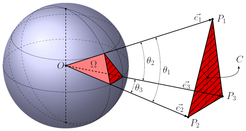
Referring to Figure 2, for the triangular region with vertices $P_1$, $P_2$, and $P_3$ and a source at O, the total luminous flux is

$$\Phi ={\int }_{\Omega }Id\Omega ={\int }_{\varphi }{\int }_{\theta }I(\theta ,\varphi )sin\theta d\theta d\varphi ,$$

(1)

and the illuminance over the triangle follows from $E=\Phi /A$, where A is the triangle area.

Since IES data are already in discrete form, a discrete evaluation is natural. For a single point-source contribution, the luminous flux is approximated as follows:

$$\Phi =I_C·\Omega ,$$

(2)

where $I_C$ is the luminous intensity in the direction from O to the triangle centroid C, and $\Omega$ is the solid angle of the triangle at O.

For the virtual-emitter model, the normalization by emitter count must be explicit because the IES file represents the complete luminaire rather than one segment of it. Let $I_{\mathrm{IES}}({\theta }_{t,k},{\varphi }_{t,k})$ be the whole-luminaire luminous intensity interpolated from the IES file in the direction from virtual emitter k to target triangle t. The normalized intensity assigned to emitter k is

$$I_{t,k}^{\left(N\right)}={\displaystyle \frac{1}{N}}{I}_{\mathrm{IES}}({\theta }_{t,k},{\varphi }_{t,k}),$$

(3)

and the simulated illuminance on triangle t becomes

$$E_t^{\mathrm{sim}}\left(N\right)={\displaystyle \frac{1}{A_t}}{\displaystyle \sum _{k=1}^N}{I}_{t,k}^{\left(N\right)}{\Omega }_{t,k}={\displaystyle \frac{1}{A_t}}{\displaystyle \sum _{k=1}^N}{\displaystyle \frac{I_{\mathrm{IES}}({\theta }_{t,k},{\varphi }_{t,k})}{N}}{\Omega }_{t,k},$$

(4)

where $A_t$ is the area of triangle t and ${\Omega }_{t,k}$ is the solid angle subtended by that triangle at virtual emitter k. This formulation preserves the total luminous intensity represented by the original IES file; increasing N changes the spatial sampling of the extended source but does not multiply the luminaire output. It also requires one IES table lookup per emitter–triangle pair while avoiding vertex-based integration over each element. A closed-form solid angle for a plane triangle [27] is used:

$$\Omega =2arctan\left({\displaystyle \frac{|{\overrightarrow{e}}_1·({\overrightarrow{e}}_2\times {\overrightarrow{e}}_3)|}{1+{\overrightarrow{e}}_1·{\overrightarrow{e}}_2+{\overrightarrow{e}}_2·{\overrightarrow{e}}_3+{\overrightarrow{e}}_3·{\overrightarrow{e}}_1}}\right),$$

(5)

where ${\overrightarrow{e}}_1$, ${\overrightarrow{e}}_2$, and ${\overrightarrow{e}}_3$ are unit vectors from O to $P_1$, $P_2$, and $P_3$. The absolute value in the numerator gives the unsigned solid-angle magnitude. This is the quantity used in the illuminance calculation because received luminous flux and illuminance are non-negative for the directly illuminated receiving side. Using unit vectors returns the exact solid angle and avoids small-angle approximations, which is important when the receiving region is tilted or the source–target geometry causes large angular extents. A signed solid angle would be useful for orientation bookkeeping, but it is not used here to assign negative illuminance.

The direction from the source to the triangle centroid, with Cartesian coordinates $(x_c,y_c,z_c)$ in the luminaire’s local frame, is expressed in spherical coordinates as follows:

$$r=\sqrt{x_c^2+y_c^2+z_c^2},\theta =arctan2(y_c,x_c),\alpha =arccos\left({\displaystyle \frac{z_c}{r}}\right).$$

(6)

When the luminaire is translated by $\overrightarrow{T}=(T_x,T_y,T_z)$ and rotated by $\mathbf{R}={\mathbf{R}}_z\left({\varphi }_z\right){\mathbf{R}}_y\left({\varphi }_y\right)$${\mathbf{R}}_x\left({\varphi }_x\right)$ [28], the transformed coordinates are

$$\left[\begin{array}{c}{x}^{\prime \prime }\\ y^{\prime \prime }\\ z^{\prime \prime }\end{array}\right]=\mathbf{R}\left[\begin{array}{c}{x}_c-T_x\\ y_c-T_y\\ z_c-T_z\end{array}\right],$$

(7)

and the updated spherical angles $({\theta }^{\prime },{\alpha }^{\prime })$ are used to evaluate $I_C$ from the IES data. Per-triangle evaluations are independent and parallelize well on modern CPUs and GPUs.

2.4. Theoretical Basis for Discretization Requirements

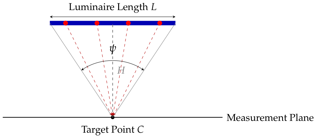
The number of virtual emitters required to faithfully reproduce the illuminance distribution of an extended source is governed by the angular subtense of the source as seen from the target plane. The representative sample schematic in Figure 3 shows the overall single-luminaire configuration used throughout this study: a linear source is positioned above a measurement plane, the source is approximated by a finite set of virtual emitters, and the contributions are evaluated at target points on the measurement grid. The dimensions and $N=4$ emitter layout in the schematic are illustrative; the actual working distance and selected emitter count are varied in the experimental cases.

For a linear luminaire of length L mounted at height H, the total angular subtense from a point directly below the luminaire center is

$$\psi =2arctan\left({\displaystyle \frac{L}{2H}}\right).$$

(8)

As H decreases relative to L, $\psi$ increases and the source occupies a larger solid angle. In this regime, the IES intensity function $I(\theta ,\varphi )$ varies significantly across the source extent, meaning that a single emitter at the luminaire center increasingly misrepresents the angular flux distribution received by target elements near the ends or off-center positions.

With N equally spaced emitters, the angular spacing between adjacent emitters is $\Delta \psi \approx \psi /N$. For the solid-angle evaluation to remain accurate, $\Delta \psi$ must be small compared to the angular scale over which $I(\theta ,\varphi )$ varies appreciably. For typical IES distributions with smooth angular falloff, this leads to the approximate scaling

$$N\sim {\displaystyle \frac{L}{H}}·C,$$

(9)

where C is a constant depending on the required accuracy and the angular gradient of the specific IES distribution. This scaling predicts that discretization requirements grow linearly with $L/H$, i.e., as the working distance decreases relative to the luminaire length. The experimental findings in Section 3 directly examine this prediction using mounting heights from 20 to $60\mathrm{cm}$ and effective source-length changes at $H=35\mathrm{cm}$. The selected emitter counts and the empirical fitted relation are presented after the single-luminaire and masked-source results, where the relation can be interpreted directly from the validation data.

The lower validity bound of the method is also established by this argument. When H approaches the scale of the internal LED pitch, diffuser structure, or other source-level features, the far-field assumption embedded in the IES file is violated not only by the overall source extent but by the discrete, spatially non-uniform nature of the source itself. The public photometric file and manufacturer information available for the tested luminaire do not report the internal LED pitch, and the diffused luminaire was not disassembled to measure it. Therefore, the LED-pitch condition is used as a physical interpretation and validity warning rather than as a fitted numerical threshold. The $H=5\mathrm{cm}$ experiment in Section 3.3.8 defines this boundary empirically for the tested luminaire and indicates when near-field goniophotometry or chip-scale ray tracing becomes necessary.

3. Experiments

The solid-angle-based illuminance calculation engine is combined here with a virtual point-light discretization approach [29] and implemented in Python with geometric processing on triangular meshes and photometric interpolation directly from IES data. The experiments are designed to answer two scientific questions: (1) Does the proposed method accurately reproduce near-field illuminance distributions from IES data? (2) How does the required emitter count N scale with the source-target geometry, specifically with $L/H$?

All experiments were conducted in a controlled, dark-room setup where the luminaire directly illuminates a flat working plane. Comprehensive architectural effects such as occlusion and multiple-bounce reflections are beyond the scope of this study.

The selected distances are not intended to represent general interior-lighting practice. They correspond to compact visual-inspection cells, in which cameras, luminaires, workpieces, shielding, and fixtures are often located within a short working distance. This is the regime in which the whole-luminaire point-source assumption in standard IES-based simulation is most likely to break down and, therefore, where a practical discretization rule is most useful.

3.1. Experimental Setup

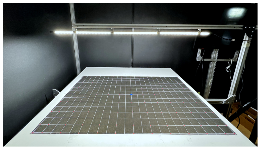
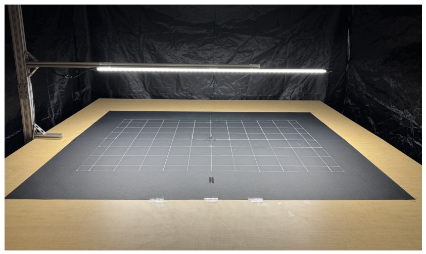
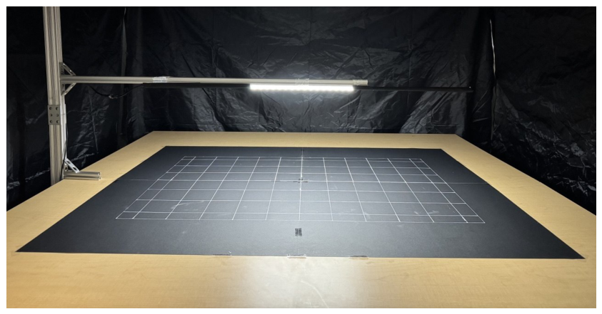
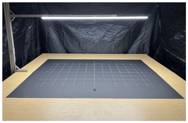
The prototype consists of a rigid fixture holding one or two luminaires at a prescribed distance above a flat table, with a gridded sheet on the table providing precisely marked measurement positions. An illuminance meter (lux meter) is placed at the marked points to record illuminance. The overall single-luminaire arrangement follows the representative sample geometry in Figure 3, while Figure 4 shows one physical implementation with the luminaire mounted at $50\mathrm{cm}$. The fixture height is adjustable to enable testing at different mounting distances.

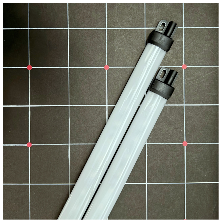
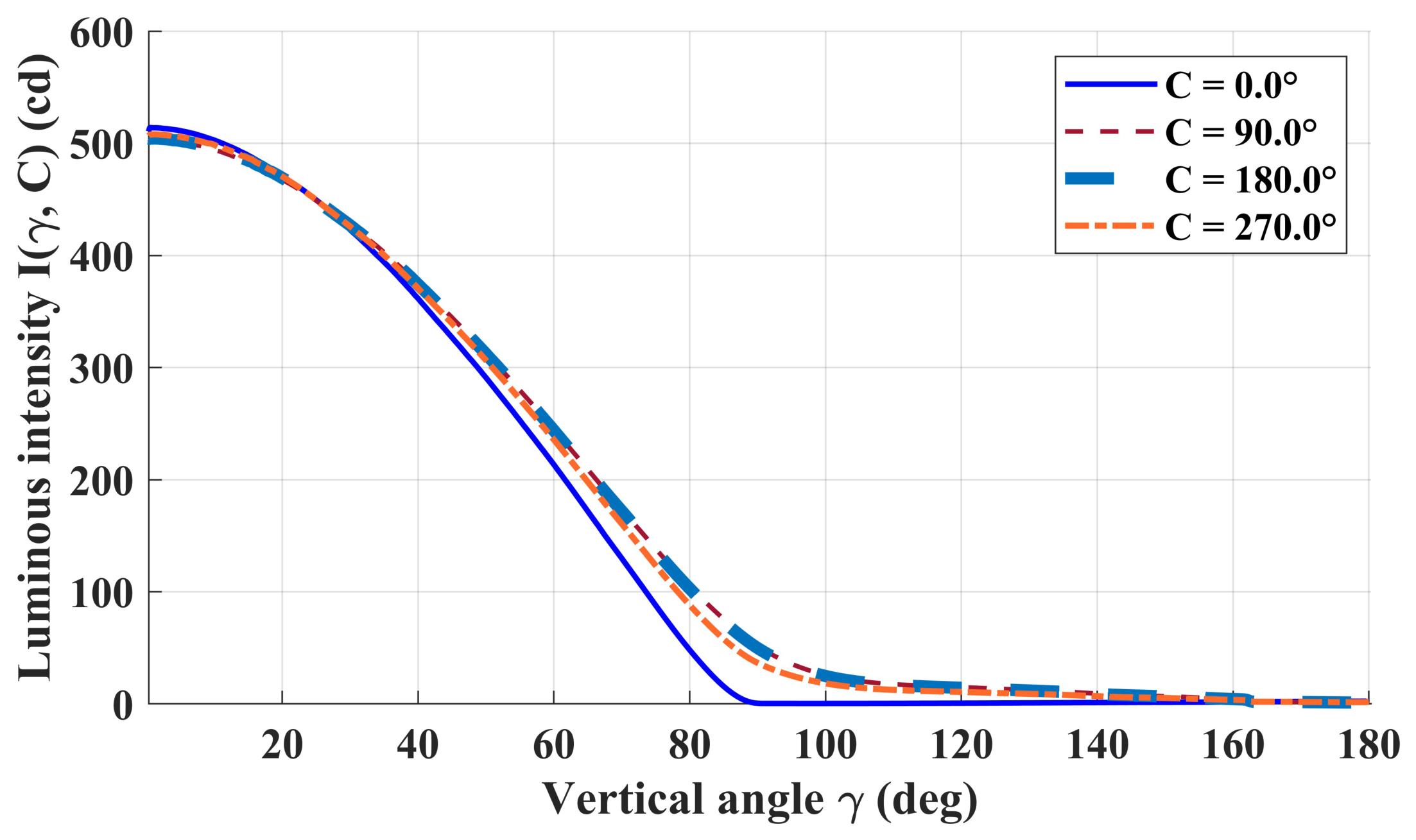
Two industrial LED luminaires from Banner Engineering (model WLS15xDW1200Dx) were used (Figure 5). Each unit is $1.2\mathrm{m}$ long, daylight-white, and designed for machine-lighting applications [30]. The luminous intensity distribution extracted from the manufacturer-provided IES file (Figure 6) shows near-rotational symmetry across C-planes ($0°$, $90°$, $180°$, $270°$) and smooth falloff with vertical angle $\gamma$, consistent with a diffuser approximating Lambertian behavior. This provides the baseline far-field photometric behavior against which near-field deviations are evaluated.

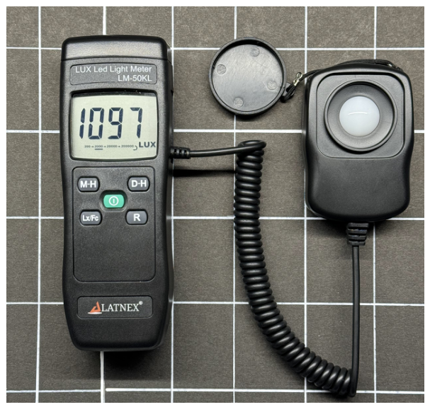
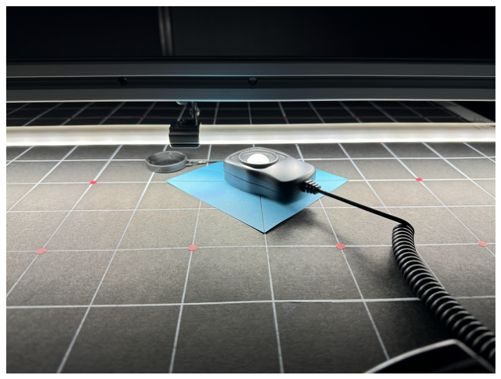
Illuminance measurements were obtained using a LATNEX LM-50KL lux meter with silicon photodiode and cosine angular correction (Figure 7). The stated accuracy is $\pm 3\%$ under calibration conditions and up to $8\%$ for other visible-light sources; cosine deviation is $\pm 0.5\%$ at $10°$, $\pm 2\%$ at $30°$, $\pm 3\%$ at $50°$, $\pm 6\%$ at $60°$, and up to $\pm 25\%$ at $80°$ [31]. All comparisons are interpreted within these instrument-limited uncertainty bounds. The effective sensor aperture was $d_{\mathrm{diff}}=20\mathrm{mm}$, well below the $50\mathrm{mm}$ grid spacing, so each reading is treated as a point sample.

The validation is intentionally limited to the tested industrial linear luminaire, which has a broad luminous-intensity distribution. Luminaires with narrow, asymmetric, or strongly lens-shaped beams may produce larger near-field errors and should be evaluated using the same candidate-emitter workflow before the selected N is transferred. The lux meter also has finite cosine-response accuracy, particularly for highly oblique rays. This limitation affects the absolute measurement uncertainty, especially near the edges of the measurement grid; however, repeated measurements and fixed sensor orientation were used to reduce random variation, and the selection of N was based on the combined behavior of MAPE, RMSE, maximum deviation, smoothness, and spatial-profile consistency, rather than on one metric alone.

To minimize geometric deformation, the fixture was attached to the luminaire housing at multiple points along its length. End-only mounting produced measurable sagging, introducing systematic illumination asymmetry that demonstrates the sensitivity of near-field measurements to luminaire straightness.

The ambient background illuminance with the test luminaire off ranged from 2 to 5 lx (slightly higher at 25 cm), small compared with the direct illuminance of several hundred to over a thousand lux. Background was measured at the center with the luminaire off and subtracted as a global offset. Spot checks at the corners confirmed $\Delta$ambient $<0.5\mathrm{lx}$ for the low-background cases. The room was dark with black-painted walls, keeping reflected contributions within experimental uncertainty.

Room temperature was controlled at approximately $24°\mathrm{C}$, and data collection commenced at least 20 min after energizing each luminaire to ensure thermal stabilization [25,26,32]. Luminaires were powered by the manufacturer-recommended constant-voltage supply with no dimming applied. A sensor alignment backplate ensured consistent placement and perpendicular orientation across the three repetitions of each experiment.

3.2. Error Metrics and Selection Criteria

For $M=117$ measurement locations, with measured illuminance $E_i^{\mathrm{meas}}$ and simulated illuminance $E_i^{\mathrm{sim}}$ at location i, the pointwise error is $e_i=E_i^{\mathrm{sim}}-E_i^{\mathrm{meas}}$. The error metrics are

$$\mathrm{RMSE}=\sqrt{{\displaystyle \frac{1}{M}}\sum _{i=1}^M{e}_i^2},{\Delta }_{max}=\underset{1\le i\le M}{max}\left|e_i\right|,\mathrm{MAPE}={\displaystyle \frac{100}{M}}{\displaystyle \sum _{i=1}^M}\left|{\displaystyle \frac{e_i}{E_i^{\mathrm{meas}}+ϵ}}\right|,$$

(10)

where $ϵ={10}^{-6}\mathrm{lx}$ avoids numerical instability. Repeatability across the three experimental runs is quantified by the mean coefficient of variation:

$$\overline{CV}={\displaystyle \frac{1}{M}}{\displaystyle \sum _{i=1}^M}{\displaystyle \frac{{\sigma }_i}{{\mu }_i}}\times 100,$$

(11)

where ${\mu }_i$ and ${\sigma }_i$ are the pointwise mean and standard deviation across repetitions.

The metrics are used to compare candidate discretizations rather than to assign a pass–fail label to each experiment. The $10\%$ MAPE level is retained as a practical engineering reference for inspection-planning accuracy, while $\overline{CV}$ indicates measurement repeatability. These values are not universal photometric tolerances; they account for the stated instrument accuracy and residual positioning uncertainty.

Smoothness of the simulated illuminance field is quantified by the mean spatial gradient magnitude R. For the candidate emitter count N, the gridded simulated illuminance is denoted $E_{i,j,N}^{\mathrm{sim}}$, where i and j are grid indices. The set $\mathcal{G}$ contains the interior grid points for which all required neighboring samples are available, and $M_g=\left|\mathcal{G}\right|$. The index-based smoothness metric used in the tables is

$$R={\displaystyle \frac{1}{M_g}}\sum _{(i,j)\in \mathcal{G}}\sqrt{{\left[{\displaystyle \frac{E_{i+1,j,N}^{\mathrm{sim}}-E_{i-1,j,N}^{\mathrm{sim}}}{2}}\right]}^2+{\left[{\displaystyle \frac{E_{i,j+1,N}^{\mathrm{sim}}-E_{i,j-1,N}^{\mathrm{sim}}}{2}}\right]}^2}.$$

(12)

Lower values of R indicate smoother spatial variation. The grid-index form is used because the measurement spacing is constant across each experiment; therefore, the reported unit remains lx for R. The final emitter-count selection is not based on scalar error alone. Candidate values of N are also checked against the measured spatial profile, and the selected value is the candidate that gives the best combined agreement, smoothness, and physically consistent centerline shape among the simulated cases.

3.3. Results

The single-luminaire experiments were processed as complete $N=1$–7 sweeps using the 117-point measurement grid, with the $H=20\mathrm{cm}$ case extended to $N=9$ as part of the expanded candidate sweep. Thus, each single-luminaire validation case now includes at least seven candidate simulations rather than relying on a single representative N value. For each case, the three measured repetitions were averaged pointwise and compared with the simulated illuminance for each candidate emitter count. The previously reported ambient values for the original experiments remain as described above. The newly added experiments were performed in a different setup, for which the ambient illuminance was less than $1\mathrm{lx}$ in all cases; this was negligible relative to the measured direct illuminance and was not a dominant contributor to the reported error metrics. The two-luminaire experiment is retained as a separate multi-source validation case and is not included in the single-luminaire discretization sweeps.

3.3.1. Single Luminaire at $H=20\mathrm{cm}$ ($L/H\approx 6.0$)

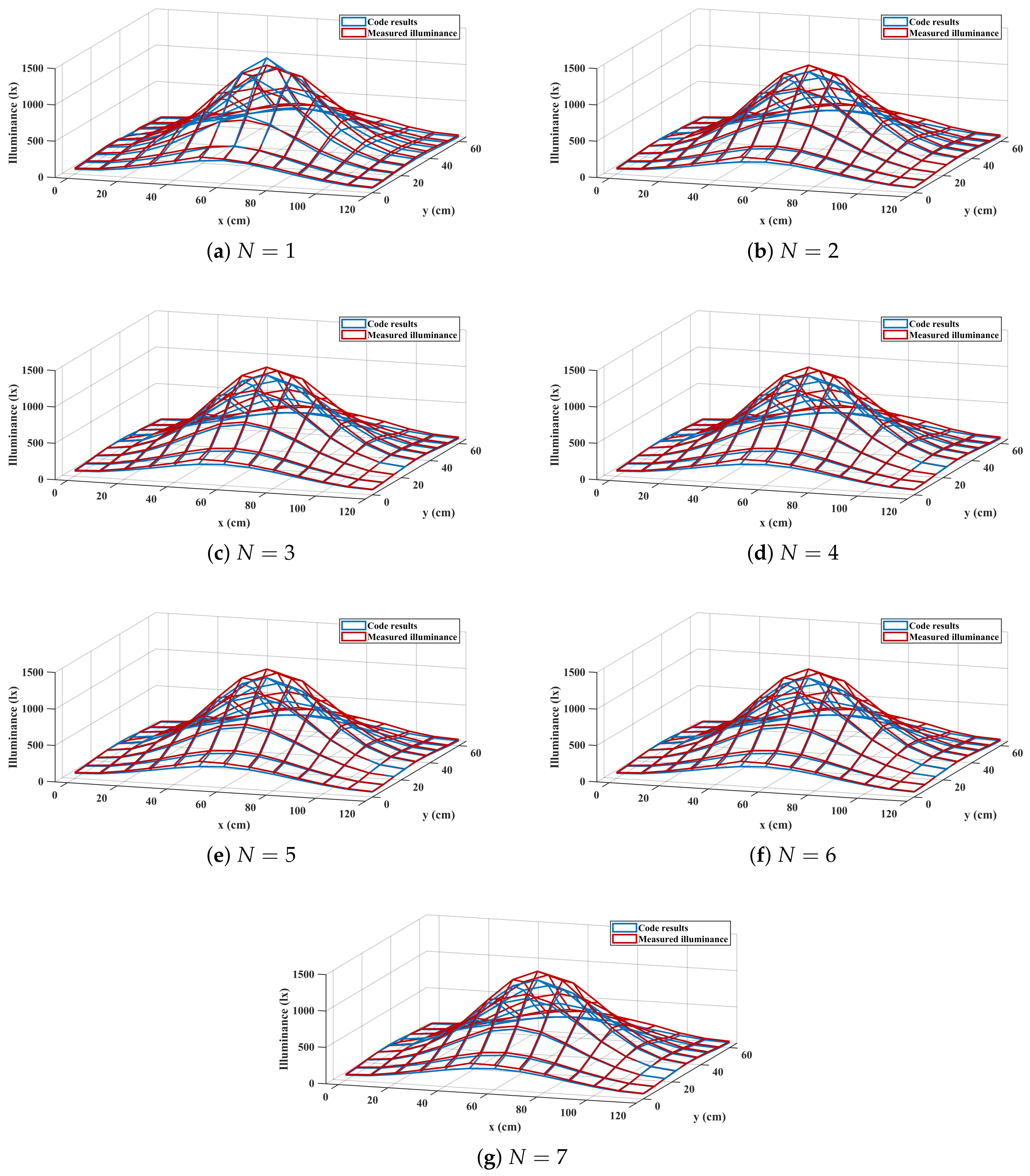
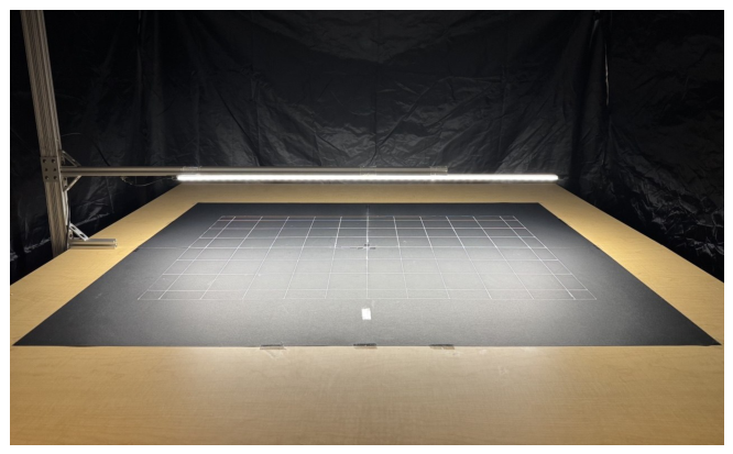
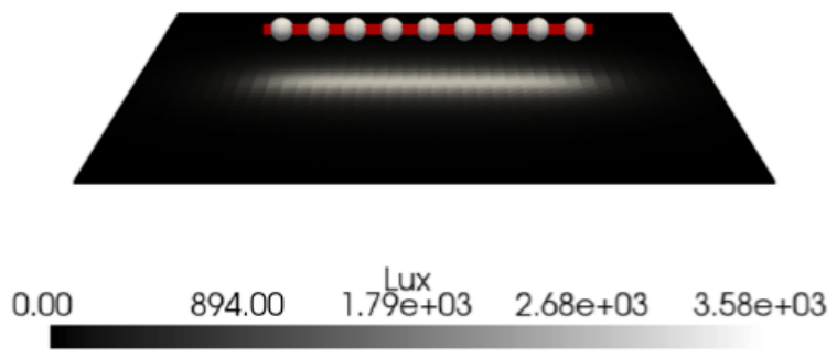
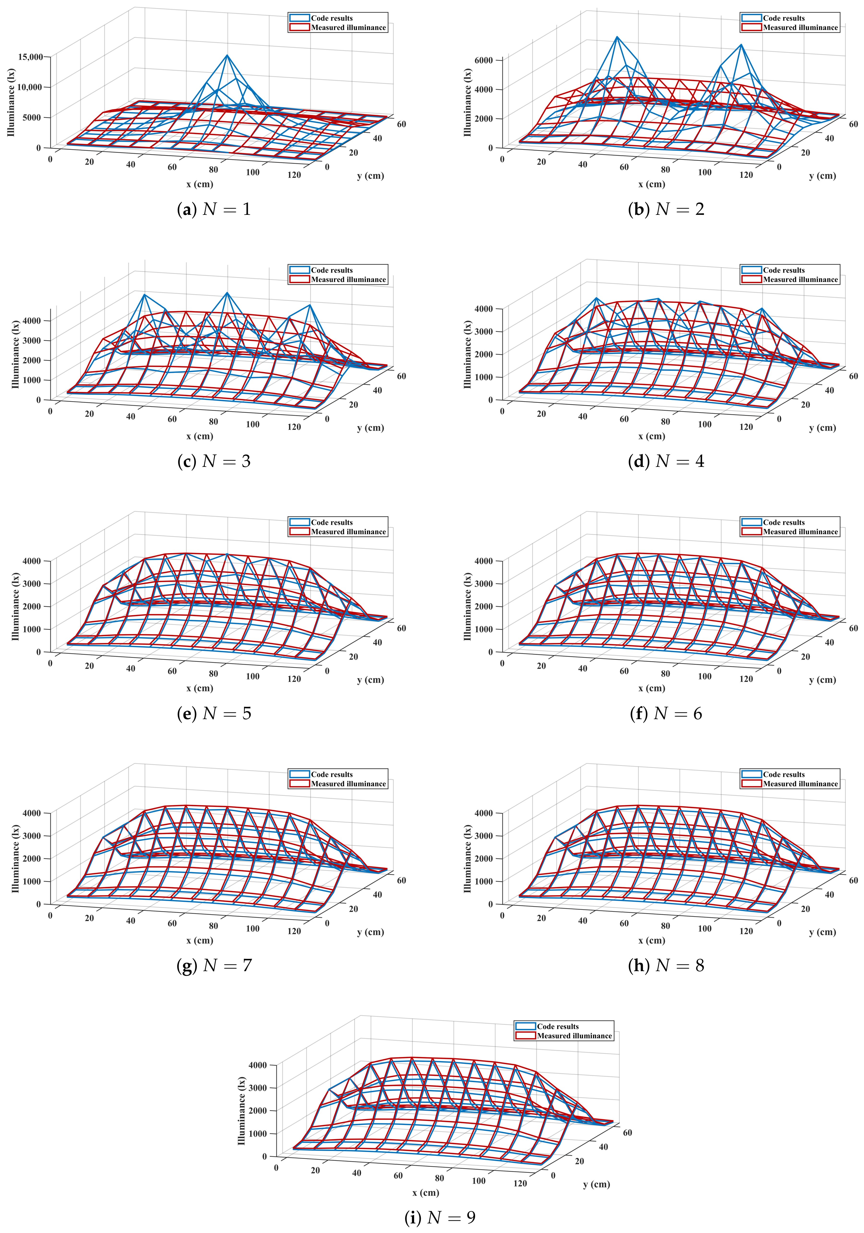
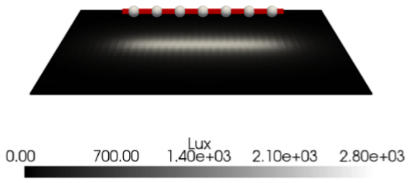
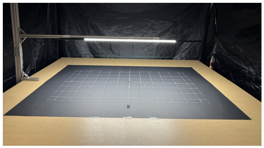
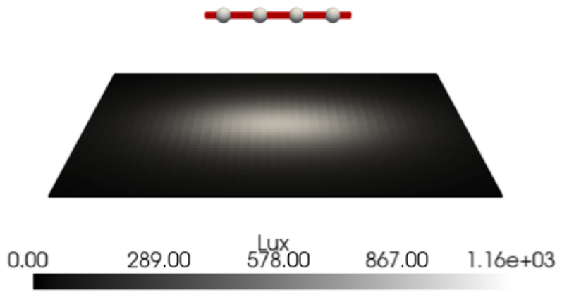
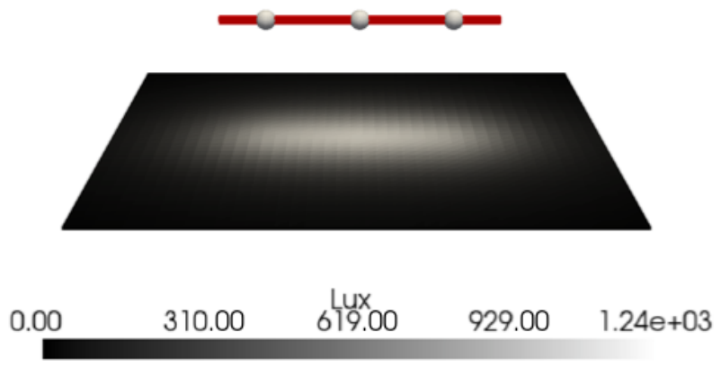
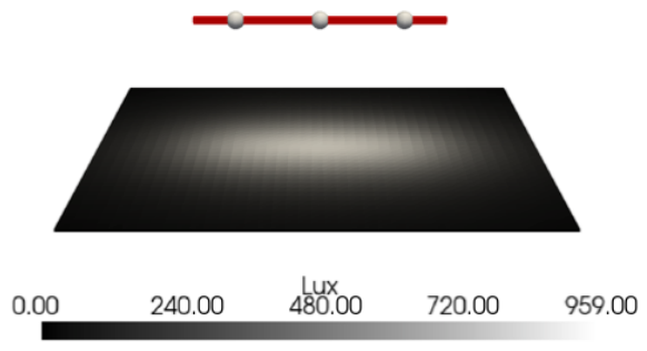
A single luminaire was mounted at $H=20\mathrm{cm}$ above the measurement plane. This case represents the strongest near-field condition in the full-grid experiments, with $L/H\approx 6.0$ for the $1.2\mathrm{m}$ luminaire. Therefore, it is expected to be the most sensitive to the number and placement of virtual emitters. The three measured repetitions gave $\overline{CV}=0.82\%$ over the 117 grid points, with a maximum pointwise CV of 3.26%. The physical setup and simulated scene are shown in Figure 8 and Figure 9, respectively, and the candidate-sweep metrics are summarized in

Table 1. Error and smoothness metrics for the single-luminaire experiment at $H=20\mathrm{cm}$. Bold indicates the selected N among the candidate simulations.

N	RMSE (lx)	MAPE (%)	${\mathbf{\Delta }}_{max}$ (lx)	R (lx)
1	1613.78	61.82	9035.13	1129.08
2	700.37	28.25	2820.76	986.26
3	326.34	18.82	1172.23	835.48
4	181.81	16.01	617.71	749.54
5	145.98	15.60	346.13	718.72
6	142.36	15.74	254.92	710.35
7	142.97	15.89	236.91	706.98
8	144.27	15.99	236.83	704.87
9	145.08	16.06	239.22	704.20

.

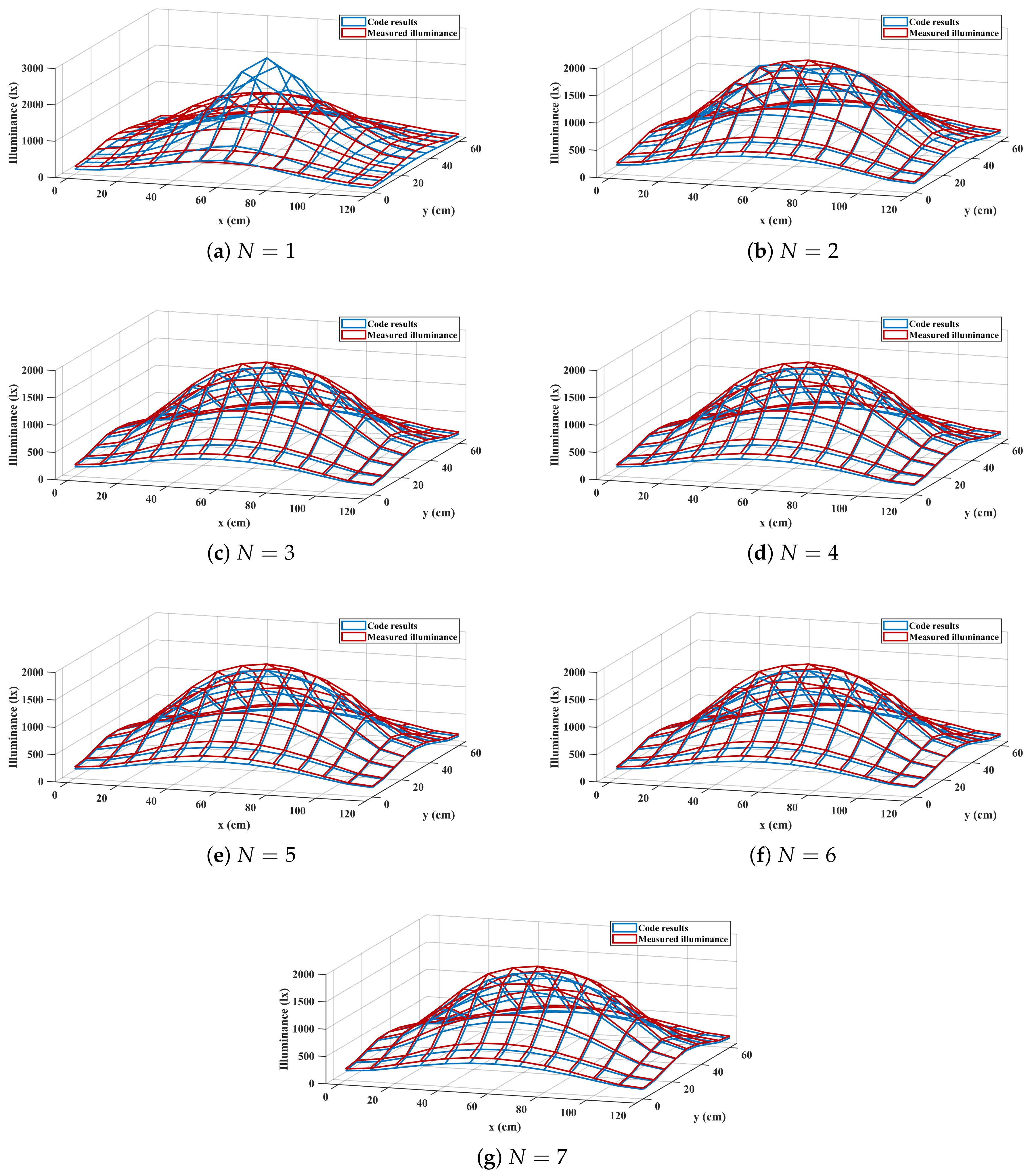
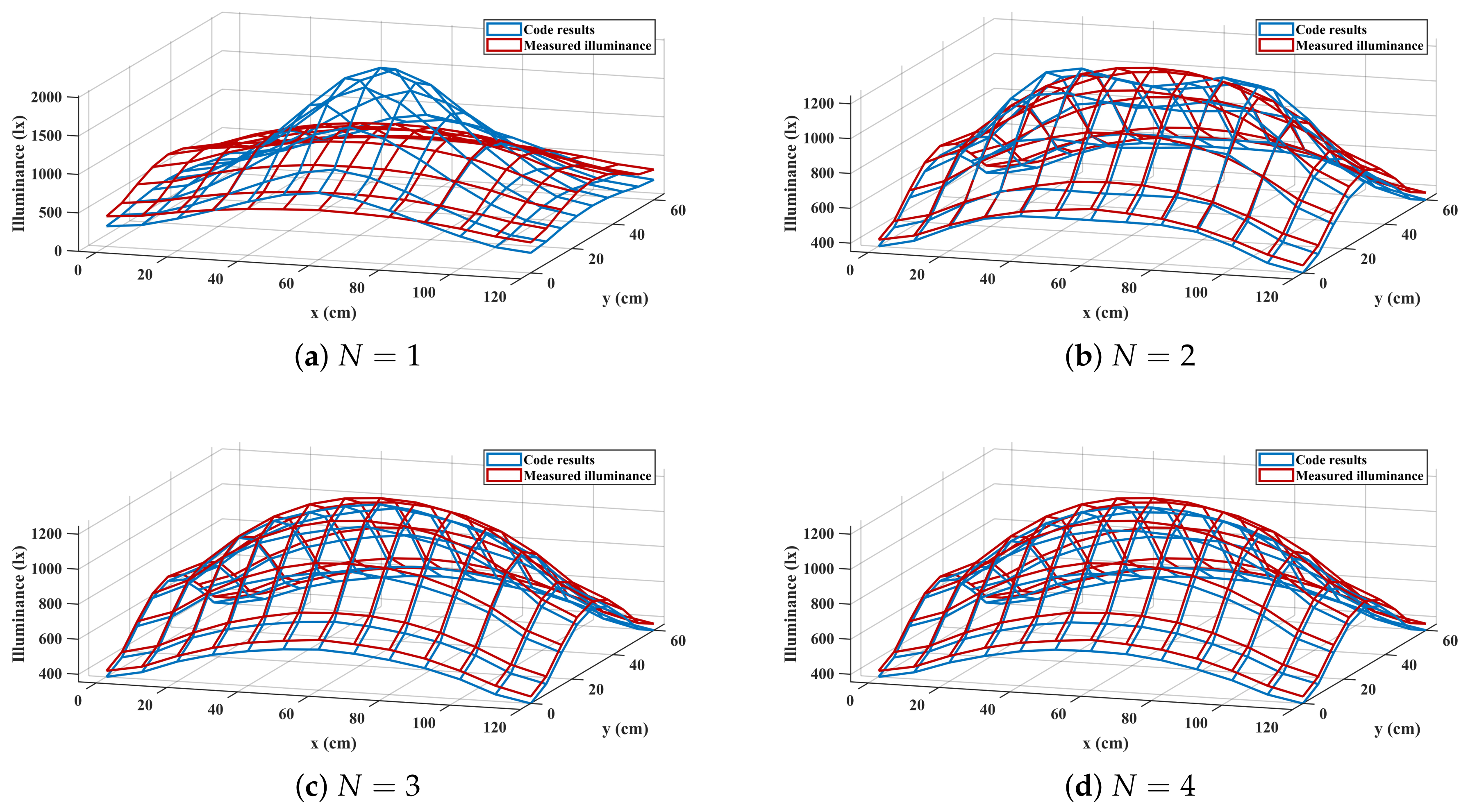
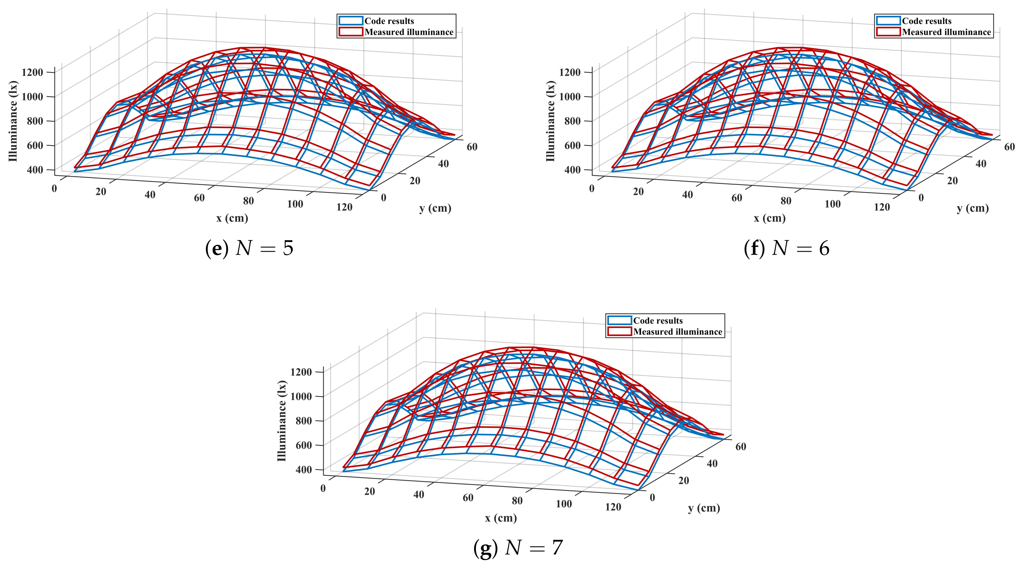
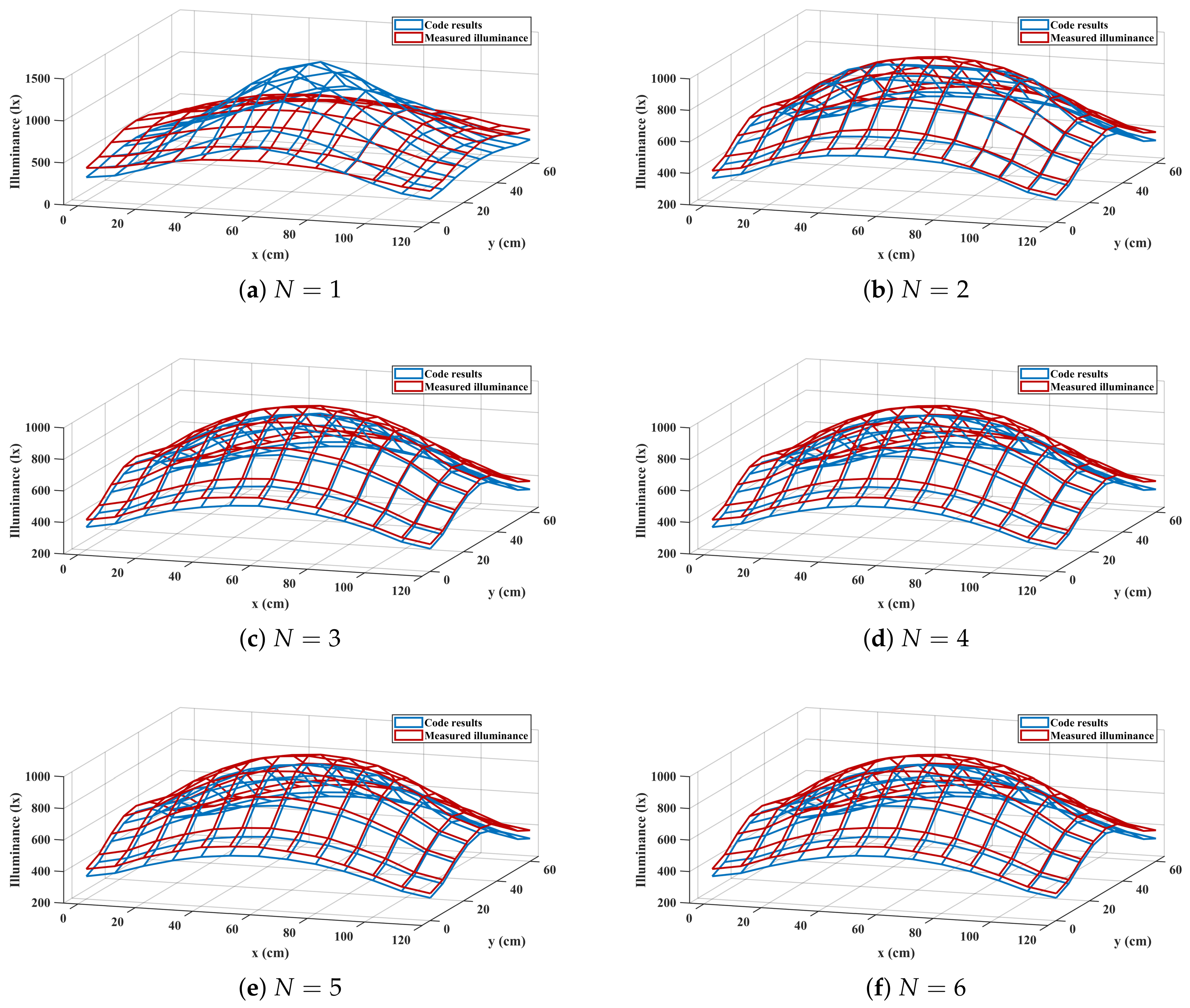
At $H=20\mathrm{cm}$, the error metrics improve sharply from $N=1$ to $N=5$ and then reach a plateau. Although $N=6$ gives the lowest RMSE, the centerline profile still shows residual oscillation caused by the discrete virtual-emitter placement. The additional $N=8$ and $N=9$ simulations have scalar error metrics close to those of $N=7$, while the smoothness metric continues to decrease. Among all tested simulations for this height, $N=9$ gives the most stable centerline representation and the smoothest illuminance field. Therefore, $N=9$ was selected as the best tested virtual-emitter count for $H=20\mathrm{cm}$. The complete measured–simulated comparison is shown in Figure 10.

3.3.2. Luminaire at $H=25\mathrm{cm}$ ($L/H\approx 4.8$)

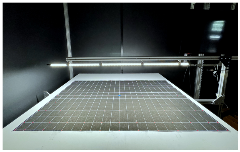
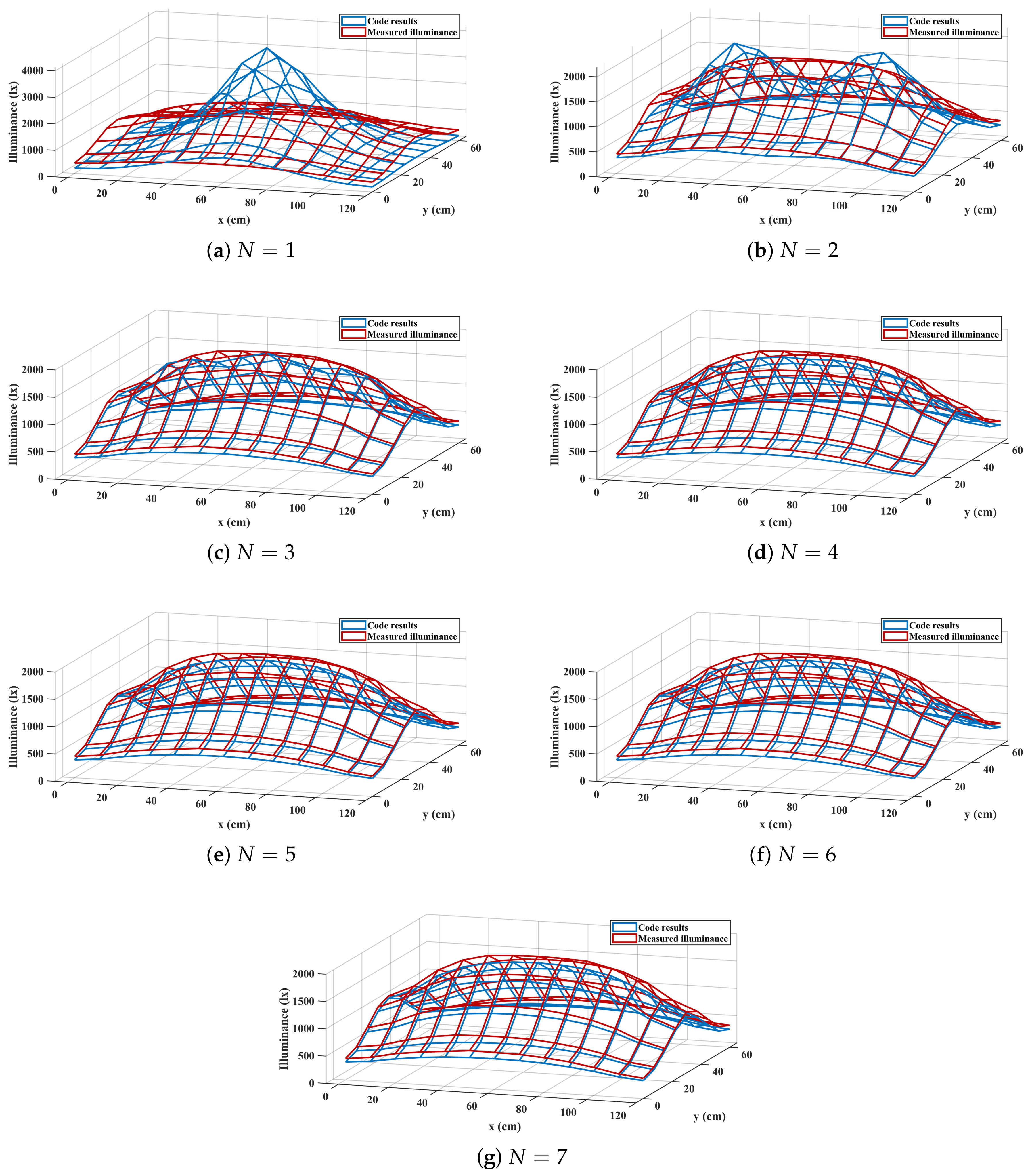
At $H=25\mathrm{cm}$, the increased $L/H$ ratio predicts a higher required emitter count than the farther-distance cases. The updated sweep evaluates $N=1$ through $N=7$ using the same 117-point grid. The three measured repetitions gave $\overline{CV}=0.47\%$ over the 117 grid points, with a maximum pointwise CV of 1.86%. The physical setup and simulated scene are shown in Figure 11 and Figure 12, respectively, and the candidate-sweep metrics are summarized in

Table 2. Error and smoothness metrics for the single-luminaire experiment at $H=25\mathrm{cm}$. Bold indicates the selected N among the candidate simulations.

N	RMSE (lx)	MAPE (%)	${\mathbf{\Delta }}_{max}$ (lx)	R (lx)
1	1130.19	56.56	5289.62	845.41
2	412.18	19.97	1474.87	690.58
3	158.23	10.94	516.12	574.34
4	88.58	9.24	244.00	531.44
5	80.60	9.20	143.83	520.80
6	81.57	9.36	135.89	517.70
7	83.14	9.52	141.02	516.15

.

For $H=25\mathrm{cm}$, $N=5$ gives the lowest RMSE and MAPE among the tested simulations. However, the $N=4$–6 profiles still contain visible oscillations and local shape reversals near the centerline, which are artifacts of under-discretizing the extended source. $N=7$ has a slightly higher MAPE than $N=5$, but it provides the smoothest and most physically consistent single-peak distribution. Therefore, $N=7$ was selected as the best candidate for this height among the simulated cases. The complete measured–simulated comparison is shown in Figure 13.

3.3.3. Single Luminaire at $H=35\mathrm{cm}$ ($L/H\approx 3.4$)

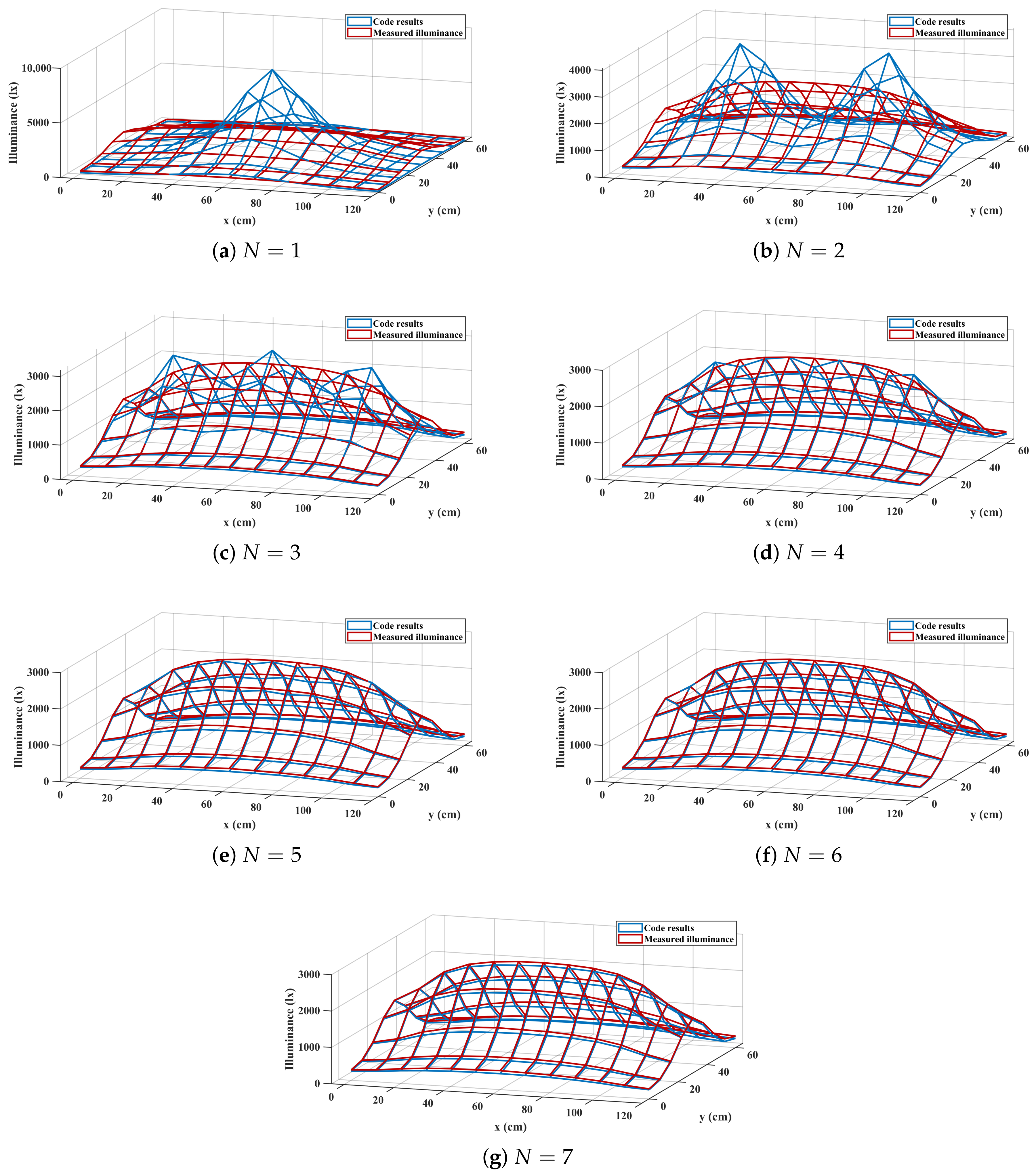
A single uncovered luminaire was mounted at $H=35\mathrm{cm}$. This intermediate height bridges the $25\mathrm{cm}$ and $50\mathrm{cm}$ cases and provides an additional point for evaluating the dependence of the required virtual-emitter count on $L/H$. The three measured repetitions gave $\overline{CV}=1.03\%$ over the 117 grid points, with a maximum pointwise CV of 8.63%. The physical setup and simulated scene are shown in Figure 14 and Figure 15, respectively, and the candidate-sweep metrics are summarized in

Table 3. Error and smoothness metrics for the uncovered single-luminaire experiment at $H=35\mathrm{cm}$. Bold indicates the selected N among the candidate simulations.

N	RMSE (lx)	MAPE (%)	${\mathbf{\Delta }}_{max}$ (lx)	R (lx)
1	605.72	43.08	2156.78	505.79
2	164.04	12.90	490.55	363.99
3	102.96	10.49	218.45	311.88
4	106.78	11.16	181.07	302.43
5	110.26	11.51	182.48	299.99
6	112.14	11.69	177.36	298.99
7	113.65	11.81	182.56	298.35

.

For the uncovered $H=35\mathrm{cm}$ case, $N=3$ provides the lowest RMSE and MAPE, but the $N=3$ and $N=4$ centerline profiles still show local oscillations that are not present in the measured field. From $N=5$ onward, the simulated distribution becomes a stable single-peak profile, while the changes in smoothness and maximum deviation are small. Therefore, $N=5$ was selected as the best candidate for this height among the simulated cases. The complete measured–simulated comparison is shown in Figure 16.

3.3.4. Single Luminaire at $H=35\mathrm{cm}$ with One Third of the Luminaire Covered

To address the effect of source length at a fixed working distance, the $H=35\mathrm{cm}$ experiment was repeated with one third of the luminaire covered in total by masking $1/6$ of the length from each side using opaque tape. The effective emitting length was approximately $0.8\mathrm{m}$, giving $L_{\mathrm{eff}}/H\approx 2.3$. The three measured repetitions gave $\overline{CV}=0.62\%$ over the 117 grid points, with a maximum pointwise CV of 9.69%. The physical setup and simulated scene are shown in Figure 17 and Figure 18, respectively, and the candidate-sweep metrics are summarized in

Table 4. Error and smoothness metrics for the $H=35\mathrm{cm}$ case with one third of the luminaire covered. Bold indicates the selected N among the candidate simulations.

N	RMSE (lx)	MAPE (%)	${\mathbf{\Delta }}_{max}$ (lx)	R (lx)
1	253.53	28.65	956.74	337.20
2	76.22	12.30	170.21	265.89
3	77.15	11.38	138.00	255.43
4	80.02	11.13	137.23	252.88
5	81.79	11.04	147.10	251.72
6	82.90	11.01	149.43	250.99
7	83.11	10.98	148.57	250.68

.

For the one-third-covered case, the lowest MAPE occurs at the largest tested N, but the improvement beyond $N=4$ is very small. $N=4$ gives nearly the same MAPE, the lowest maximum local deviation, and a lower computational cost. Therefore, $N=4$ was selected as the best practical candidate for this masked-source case among the simulated values. The complete measured–simulated comparison is shown in Figure 19.

3.3.5. Single Luminaire at $H=35\mathrm{cm}$ with Two Thirds of the Luminaire Covered

The fixed-height source-length study was further extended by covering two thirds of the luminaire in total, masking $1/3$ of the length from each side. The effective emitting length was approximately $0.4\mathrm{m}$, giving $L_{\mathrm{eff}}/H\approx 1.1$ at $H=35\mathrm{cm}$. The three measured repetitions gave $\overline{CV}=1.56\%$ over the 117 grid points, with a maximum pointwise CV of 60.75%. The physical setup and simulated scene are shown in Figure 20 and Figure 21, respectively, and the candidate-sweep metrics are summarized in

Table 5. Error and smoothness metrics for the $H=35\mathrm{cm}$ case with two thirds of the luminaire covered. Bold indicates the selected N among the candidate simulations.

N	RMSE (lx)	MAPE (%)	${\mathbf{\Delta }}_{max}$ (lx)	R (lx)
1	51.69	14.98	130.15	168.60
2	48.21	11.14	128.28	155.53
3	50.67	10.74	136.35	153.76
4	51.99	10.66	148.27	152.97
5	52.16	10.60	146.49	152.83
6	52.38	10.58	150.04	152.67
7	52.48	10.57	149.45	152.62

.

For the two-thirds-covered case, increasing N slightly reduces MAPE but does not reduce RMSE or the maximum local deviation. Because the effective source is much shorter, $N=2$ gives the best balance of accuracy, smoothness, and computational cost among the tested simulations. This supports the interpretation that reducing the effective source length reduces the required emitter count. The complete measured–simulated comparison is shown in Figure 22.

3.3.6. Luminaire at $H=50\mathrm{cm}$ ($L/H\approx 2.4$)

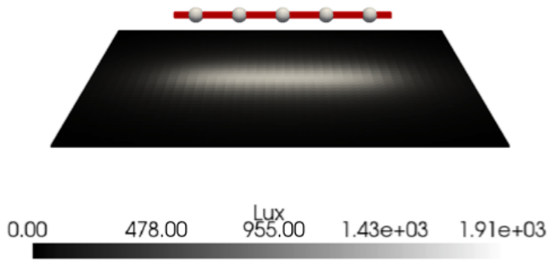
One luminaire was placed at $H=50\mathrm{cm}$, facing downward. This case represents a moderate near-field configuration and was part of the original validation set. The three measured repetitions gave $\overline{CV}=0.32\%$ over the 117 grid points, with a maximum pointwise CV of 1.39%. The physical setup and simulated scene are shown in Figure 4 and Figure 23, respectively, and the candidate-sweep metrics are summarized in

Table 6. Error and smoothness metrics for the single-luminaire experiment at $H=50\mathrm{cm}$. Bold indicates the selected N among the candidate simulations.

N	RMSE (lx)	MAPE (%)	${\mathbf{\Delta }}_{max}$ (lx)	R (lx)
1	271.32	27.93	775.12	254.56
2	45.18	5.41	106.97	164.18
3	41.46	5.70	61.82	152.45
4	46.62	6.38	64.66	150.19
5	48.84	6.66	66.53	149.37
6	49.98	6.80	67.77	149.02
7	50.85	6.90	68.03	148.70

.

At $H=50\mathrm{cm}$, $N=2$ gives the lowest MAPE but has a larger maximum local deviation and the same type of under-discretized centerline artifact observed in the farther-distance two-emitter case. $N=3$ gives the lowest RMSE, substantially reduces the maximum deviation, and provides a stable single-peak profile. Therefore, $N=3$ was selected as the best candidate for this height among the simulated cases. The complete measured–simulated comparison is shown in Figure 24.

3.3.7. Single Luminaire at $H=60\mathrm{cm}$ ($L/H\approx 2.0$)

A single luminaire was also tested at $H=60\mathrm{cm}$. This is the largest working distance in the single-luminaire validation set and, therefore, has the smallest $L/H$ ratio among the uncovered cases. The three measured repetitions gave $\overline{CV}=0.25\%$ over the 117 grid points, with a maximum pointwise CV of 0.81%. The physical setup and simulated scene are shown in Figure 25 and Figure 26, respectively, and the candidate-sweep metrics are summarized in

Table 7. Error and smoothness metrics for the single-luminaire experiment at $H=60\mathrm{cm}$. Bold indicates the selected N among the candidate simulations.

N	RMSE (lx)	MAPE (%)	${\mathbf{\Delta }}_{max}$ (lx)	R (lx)
1	162.70	20.34	417.02	167.41
2	39.83	5.91	71.57	106.61
3	47.87	7.38	73.46	101.71
4	51.86	7.96	78.04	100.37
5	53.49	8.20	80.38	99.86
6	54.35	8.31	79.41	99.60
7	54.96	8.39	81.84	99.39

.

For $H=60\mathrm{cm}$, $N=2$ provides the lowest RMSE, MAPE, and maximum local deviation among the tested simulations. However, the $N=2$ comparison shows a small nonphysical dip near the middle of the centerline profile, rather than the smooth single maximum observed in the measurements. $N=3$ removes this artifact and improves the gradient-based smoothness metric. Therefore, $N=3$ was selected as the best profile-consistent value for the farthest tested single-luminaire case. The complete measured–simulated comparison is shown in Figure 27.

The selected emitter counts follow the expected trend for the uncovered luminaire once profile stability is included: the selected value decreases from $N=9$ at $H=20\mathrm{cm}$ to $N=7$ at $H=25\mathrm{cm}$, and then to $N=5$ at $H=35\mathrm{cm}$ and $N=3$ at $H=50$–$60\mathrm{cm}$. This trend is more conservative than choosing the minimum scalar error alone, because low emitter counts can yield favorable RMSE or MAPE while producing nonphysical centerline oscillations. The masked-source cases support the same geometric interpretation: reducing the effective emitting length at fixed height reduces the practical emitter count from the uncovered $H=35\mathrm{cm}$ case to $N=4$ for one-third coverage and $N=2$ for two-thirds coverage.

The three $H=35\mathrm{cm}$ cases isolate the effect of changing the effective source length while keeping the working distance fixed. The uncovered luminaire has $L_{\mathrm{eff}}=1.2\mathrm{m}$ and selected $N=5$; covering one third of the source reduces $L_{\mathrm{eff}}$ to approximately $0.8\mathrm{m}$ and selected N to 4; covering two thirds reduces $L_{\mathrm{eff}}$ to approximately $0.4\mathrm{m}$ and selected N to 2. This fixed-height comparison confirms that the discretization requirement is controlled not only by H but by the ratio of effective emitting length to working distance, as predicted by the angular-subtense argument.

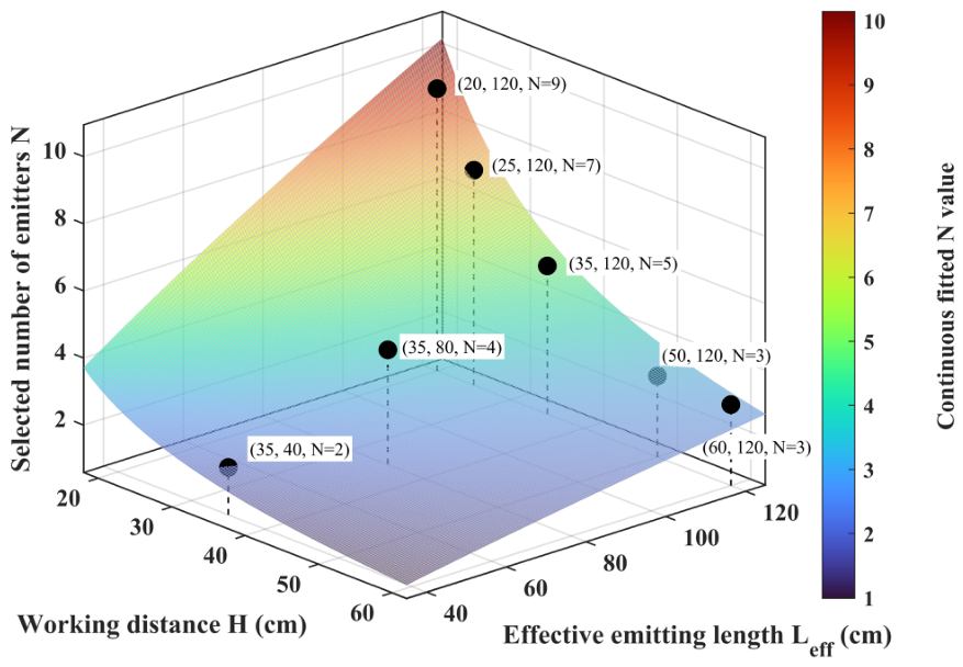
Using all selected cases in

Table 8. Selected virtual-emitter count for the single-luminaire and masked-source validation cases.

Case	$\mathit{L}/\mathit{H}$ or ${\mathit{L}}_{\mathbf{eff}}/\mathit{H}$	$\overline{\mathit{CV}}$ (%)	Selected N	RMSE (lx)	MAPE (%)
$H=20\mathrm{cm}$	6.0	0.82	9	145.08	16.06
$H=25\mathrm{cm}$	4.8	0.47	7	83.14	9.52
$H=35\mathrm{cm}$	3.4	1.03	5	110.26	11.51
$H=35\mathrm{cm}$, 1/3 covered	2.3 eff.	0.62	4	80.02	11.13
$H=35\mathrm{cm}$, 2/3 covered	1.1 eff.	1.56	2	48.21	11.14
$H=50\mathrm{cm}$	2.4	0.32	3	41.46	5.70
$H=60\mathrm{cm}$	2.0	0.25	3	47.87	7.38

, a two-variable power-law fit was obtained for estimating the selected emitter count:

$$N_{\mathrm{sel}}\approx \mathrm{round}\left[4.93L_{\mathrm{eff},\mathrm{cm}}^{0.79}{H}_{\mathrm{cm}}^{-1.07}\right],$$

(13)

where $L_{\mathrm{eff},\mathrm{cm}}$ and $H_{\mathrm{cm}}$ are the numerical values of the effective emitting length and working distance expressed in centimeters, respectively. The coefficient in Equation (13) is therefore tied to centimeter units; if another unit system is used, the coefficient must be converted or the relation must be refitted. The exponent magnitude for $H_{\mathrm{cm}}$ is slightly larger than that for $L_{\mathrm{eff},\mathrm{cm}}$, indicating that the working distance has the stronger influence within the tested range. Because the relation is fitted from the selected simulations in this study, it should be used as an interpolation guideline for comparable linear luminaires and similar near-field inspection geometries rather than as a universal photometric law. Figure 28 visualizes the fitted surface and the selected data points.

3.3.8. Establishing the Validity Boundary: Luminaire at $H=5\mathrm{cm}$

A complete characterization of the proposed method requires identifying not only the conditions under which it succeeds but also the physical limit beyond which IES-based simulation is fundamentally inapplicable. At $H=5\mathrm{cm}$, the source-to-target distance is very small compared with the luminaire length ($L/H=24$) and approaches the scale at which internal LED spacing, diffuser structure, and local source non-uniformities become visible in the measured field. The public datasheet and IES file for the tested luminaire do not report the internal LED pitch, and the luminaire was not disassembled because doing so would alter the optical system. Therefore, the pitch is not used as a numerical input in the model. Instead, the $H=5\mathrm{cm}$ test is used as an empirical failure case showing that, at sufficiently small distances, the far-field IES representation is violated not only by overall source extent but by source-level spatial non-uniformity that whole-luminaire IES data cannot capture.

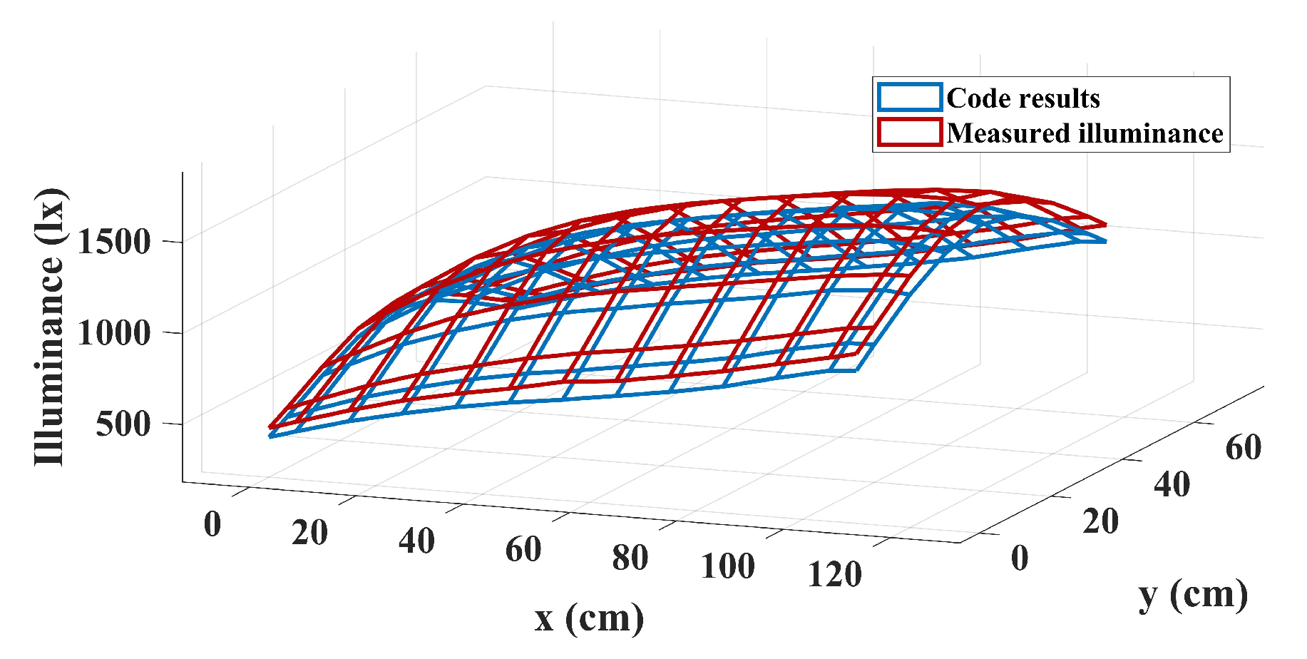
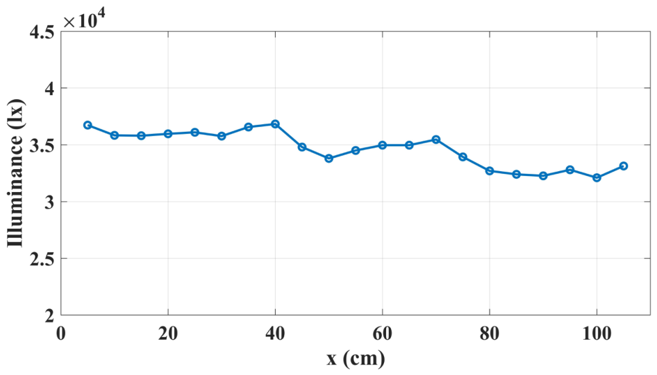
Illuminance values were measured along a straight line parallel to the luminaire at 21 points, repeated three times (Figure 29). The resulting distribution (Figure 30) deviates from the smooth arc expected of a uniform extended source, revealing LED-to-LED output differences and mechanical non-uniformities. These imperfections become significant error sources precisely because the IES model cannot represent individual emitter positions.

This experiment defines the practical lower bound of the proposed method for the tested luminaire: IES-based simulation is appropriate only while H remains large enough that source-level non-uniformities are averaged by the optical system and are not individually resolved at the target plane. If the LED pitch or diffuser structure is available from manufacturer data, it can be used as a useful warning scale. If it is not available, as in the present case, the limitation should be identified by a short-distance validation test. Below this boundary, near-field goniophotometry or chip-scale ray tracing is required. This finding provides practitioners with a physically motivated criterion for selecting the appropriate modeling approach, rather than discovering its limitations through trial and error.

3.3.9. Generalization to a Second Luminaire

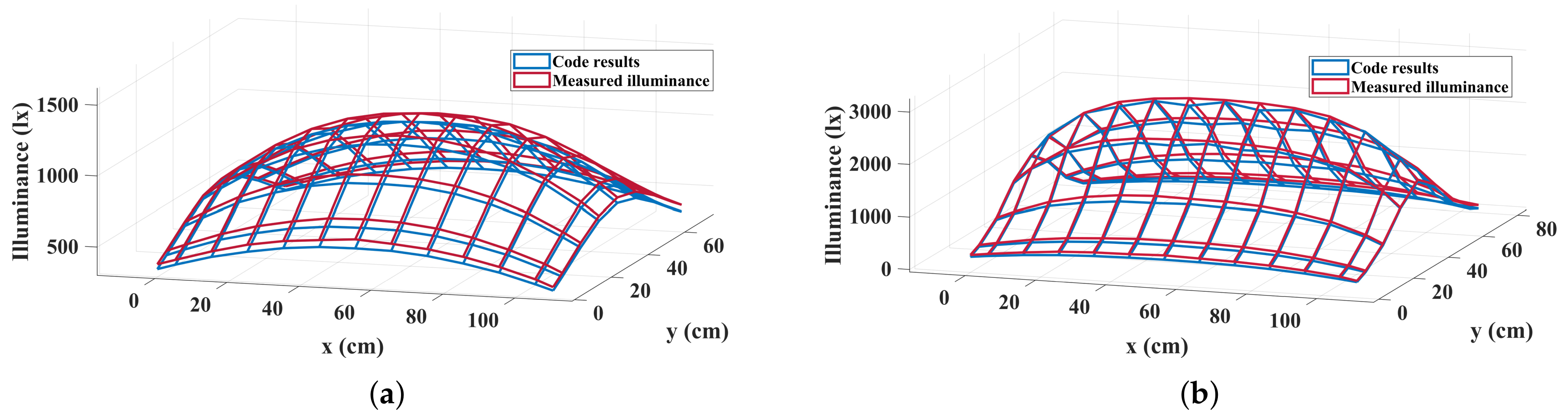
To examine whether the method and emitter-count guidelines transfer to a different unit of the same model, all experiments were repeated with the second Banner Engineering WLS15xDW1200Dx luminaire. The results are shown in Figure 31. At $H=50\mathrm{cm}$, the mean error is $6.2\%$ ($N=4$); at $H=25\mathrm{cm}$, the original transfer check gives $9.2\%$ with $N=5$. These results are within the same accuracy range as the first luminaire. The updated profile-stability criterion remains more conservative for the full single-luminaire sweep, where higher N values are selected when lower emitter counts create visible centerline oscillations.

3.3.10. Two-Luminaire Configuration

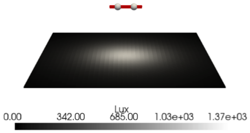
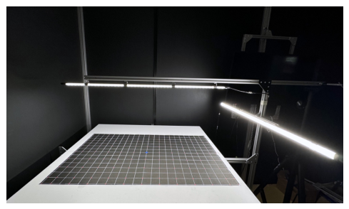
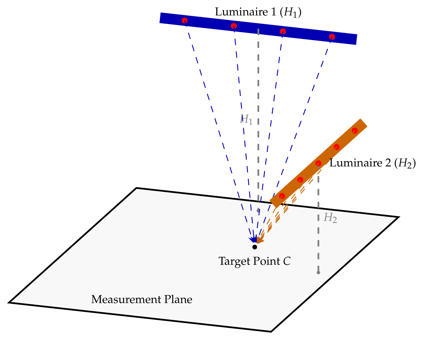
The final experiment evaluated the method in a multi-source configuration with arbitrary orientation. One luminaire was mounted at $H=50\mathrm{cm}$ facing the working plane; a second was mounted perpendicular to the first at $H=30\mathrm{cm}$, oriented $90°$ to the plane (Figure 32). These two different heights and orientations were chosen deliberately to create a more demanding validation case than two identical, co-planar, equal-height sources. The purpose was to test whether the same coordinate transformation, IES lookup, solid-angle evaluation, and superposition procedure remain valid when luminaires contribute from different positions, directions, and source–target distances. Four point-lights were used for the $50\mathrm{cm}$ luminaire and five for the $30\mathrm{cm}$ perpendicular one, following the criteria established in earlier experiments. The optical-path schematic used for this two-luminaire simulation is shown in Figure 33.

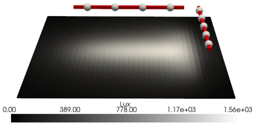
The corresponding simulated scene for this multi-source configuration is shown in Figure 34.

Simulated and measured illuminance are compared in Figure 35. The overall mean error across all 117 points is $6.9\%$. The simulated distribution correctly captures the asymmetric illuminance pattern, with the highest values in the region receiving flux from both luminaires. These results confirm that the workflow generalizes to multi-source, differently oriented configurations without modification.

3.4. Method Comparison

Table 9. Comparison of illuminance modeling approaches for extended industrial luminaires. Representative references are included for each method family.

Method	Representative References	Input Required	Comp. Cost	Near-Field Accuracy	Data Availability
Point-source IES ($N=1$)	[2,3,16,25,26]	IES file	Very low	Poor at $H<L$	Universal
Proposed (selected $\mathbf{N}=\mathbf{2}$–9)		IES file	Low	Good agreement in tested range	Universal
Monte Carlo ray tracing	[19]	Geometric + optical model	Very high	Excellent	Specialist software
Near-field goniophotometry	[4,5]	Lab measurement	N/A	Reference quality	Rarely available
Analytic Lambertian	[24]	Assumed luminance	Very low	Poor for LED luminaires	Universal

positions the proposed method relative to alternative approaches and lists representative references for each method family. The proposed method occupies the practical middle ground between the inaccurate but universally applicable point-source approximation and the accurate but resource-intensive ray tracing and goniophotometric approaches, making it particularly suited to inspection cell commissioning where design iteration speed is prioritized. Commercial optical-design packages such as Speos or Photopia are more appropriate when detailed source geometry, optical materials, diffuser properties, and ray-level source data are available. The proposed workflow is not intended to replace those validated tools; rather, it fills the lower-data planning case in which only a manufacturer IES file and luminaire dimensions are available.

4. Conclusions

This study introduces and validates a solid-angle-based workflow for simulating direct near-field illumination from extended industrial luminaires using triangular meshes and standard IES photometric data. Three transferable scientific findings are established:

• Discretization scales mainly with working distance and effective length. The ratio of luminaire length to working height is the primary geometric parameter governing emitter count requirements. An angular-subtense argument predicts approximately linear scaling $N\sim (L/H)·C$, examined experimentally through an expanded sweep at $H=20\mathrm{cm}$, $25\mathrm{cm}$, $35\mathrm{cm}$, $50\mathrm{cm}$, and $60\mathrm{cm}$ and two masked-source cases at $H=35\mathrm{cm}$. The uncovered single-luminaire experiments show that the selected emitter count decreases from $N=9$ at $H=20\mathrm{cm}$ to $N=7$ at $H=25\mathrm{cm}$, and then to $N=5$ at $H=35\mathrm{cm}$ and $N=3$ at $H=50$–$60\mathrm{cm}$. The fixed-height masked-source tests at $H=35\mathrm{cm}$ confirm that reducing $L_{\mathrm{eff}}$ from 1.2 m to approximately 0.8 m and 0.4 m reduces the selected emitter count from $N=5$ to $N=4$ and $N=2$, respectively. The empirical fit in Equation (13) indicates a stronger dependence on working distance H than on effective source length $L_{\mathrm{eff}}$ within the tested range.
• The validity boundary is physically motivated. IES-based simulation becomes unreliable when H approaches the scale of internal source features such as LED pitch, diffuser structure, or package-level non-uniformity. For the tested luminaire, the internal pitch was not publicly reported, so the $H=5\mathrm{cm}$ experiment was used as an empirical lower-bound demonstration. This criterion provides guidance for selecting between IES-based discretization and more detailed near-field goniophotometry or chip-scale ray tracing.
• The solid-angle formulation is computationally efficient and geometrically general. The closed-form per-triangle evaluation reduces IES table queries by a factor proportional to mesh density compared with vertex-based schemes, while naturally extending to arbitrary 3D meshes and multi-source, arbitrarily oriented configurations.

The main methodological contribution is a reproducible workflow for selecting the best practical emitter count for a specified luminaire, working distance, measurement grid, and error criterion, demonstrated across one and two luminaires. The expanded single-luminaire sweep shows how the selected N changes systematically with H and $L_{\mathrm{eff}}$, with $N=9$, 7, 5, 3, and 3 selected for the uncovered cases from $H=20$ to $60\mathrm{cm}$ and lower values selected when the effective source length is reduced at fixed height. The workflow is not limited to the tested luminaire: an engineer can repeat the discretization sweep and error evaluation for any luminaire for which an IES file is available.

The practical utility of the proposed method can be summarized as follows:

• Rapid Inspection-Cell Lighting Layout: It enables engineers to estimate direct illuminance and spatial coverage during early fixture design using only a manufacturer IES file, luminaire dimensions, source pose, and a target mesh, without first constructing a detailed optical model of LEDs, lenses, reflectors, or diffusers.
• Selection of Mounting Height and Source Discretization: By sweeping the number of virtual emitters at the intended working distance, the method helps determine when a single IES point source is inadequate and what discretization level gives a stable engineering approximation for the specific source–target geometry.
• Comparison of Alternative Luminaire Placements and Orientations: The same calculation can be repeated for candidate source locations, mounting heights, orientations, and multi-luminaire arrangements, allowing illumination configurations to be ranked before physical installation or prototype fabrication.
• Evaluation of Illumination on Nontrivial Target Geometry: Because the illuminance calculation is performed on triangular mesh elements using closed-form solid-angle evaluation, the framework can be applied to discretized 3D workpieces and inspection regions rather than being restricted to a single analytical plane.
• Screening for Coverage and Uniformity Problems before Camera Deployment: Predicted low-illuminance regions, strong gradients, and non-uniform coverage can be identified early, supporting decisions on light placement, shielding, fixturing, and camera pose in machine-vision inspection systems.
• Decision Support for Higher-Fidelity Characterization: The method provides a computationally inexpensive intermediate step between a single far-field IES point source and specialist approaches such as near-field goniophotometry or chip-scale Monte Carlo ray tracing. Large residual errors or failure to obtain a stable discretization can therefore be used as evidence that more detailed source characterization is warranted.

The formulation is limited to direct illumination on planar benchmarks; extensions to fully 3D targets, occlusion, interreflections, and diffuser-specific near-field characterization are important next steps. In future work, the illumination method presented in the current paper will be combined with the FASTVIS occlusion-detection framework [33] to develop a fast simulation workflow for inspection scenes that accounts for both direct illumination and geometric visibility. Additional extensions include dynamic sources, secondary light transport, and luminaire-specific near-field characterization.

References

1. Commission Internationale de l’Éclairage (CIE). CIE 070-1987: The Measurement of Absolute Luminous Intensity Distributions; CIE: Vienna, Austria, 1987. [Google Scholar]
2. Commission Internationale de l’Éclairage (CIE). CIE 121-1996: The Photometry & Goniophotometry of Luminaires; CIE: Vienna, Austria, 1996. [Google Scholar]
3. Illuminating Engineering Society. ANSI/IES LM-75-19: Approved Method: Guide to Goniometer Measurements and Types, and Photometric Coordinate Systems; IES: New York, NY, USA, 2019. [Google Scholar]
4. Ohno, Y. Overview of Near-Field Goniophotometry and Its Applications. In Proceedings of the CIE Conference, Budapest, Hungary, 23–27 June 2014. [Google Scholar]
5. Simonot, L.; Reux, F.; Carré, S.; Martinsons, C. The usefulness of near-field goniophotometry data to assess illuminances and discomfort glare in indoor lighting. Leukos 2022, 18, 246–257. [Google Scholar]
6. Komarsofla, A.K.; Charest-Finn, M.; Nokleby, S. Autonomous Inspection of Steel Pipe Weld Lines Implementing Frequency Analysis Combined with YOLOv5. In Proceedings of the Canadian Society for Mechanical Engineering International Congress, Sherbrooke, QC, Canada, 28–31 May 2023. [Google Scholar]
7. García-Chamizo, J.M.; Fuster-Guilló, A.; Azorín-López, J. Simulation of automated visual inspection systems for specular surfaces quality control. In Proceedings of the Pacific-Rim Symposium on Image and Video Technology; Springer: Berlin/Heidelberg, Germany, 2007; pp. 749–762. [Google Scholar]
8. Kuric, I.; Klarák, J.; Bulej, V.; Sága, M.; Kandera, M.; Hajdučík, A.; Tucki, K. Approach to automated visual inspection of objects based on artificial intelligence. Appl. Sci. 2022, 12, 864. [Google Scholar] [CrossRef]
9. Kuo, C.-F.J.; Fang, T.-Y.; Lee, C.-L.; Wu, H.-C. Automated optical inspection system for surface mount device light emitting diodes. J. Intell. Manuf. 2019, 30, 641–655. [Google Scholar]
10. Fu, G.; Jia, S.; Zhu, W.; Yang, J.; Cao, Y.; Yang, M.Y.; Cao, Y. Fusion of multi-light source illuminated images for effective defect inspection on highly reflective surfaces. Mech. Syst. Signal Process. 2022, 175, 109109. [Google Scholar] [CrossRef]
11. Parrott, E.; Pickard, J.K.; Dubay, R. Synthesis of Valid Camera Poses for the Inspection of Triangular Facets in a 3D Mesh. Sensors 2023, 23, 7878. [Google Scholar] [CrossRef] [PubMed]
12. Parrott, E.; Pickard, J.K.; Dubay, R. Practical Applications of a Set-Based Camera Deployment Methodology. Sensors 2023, 24, 111. [Google Scholar] [CrossRef] [PubMed]
13. Zhou, L.; Zhang, L.; Konz, N. Computer Vision Techniques in Manufacturing. IEEE Trans. Syst. Man Cybern. Syst. 2023, 53, 105–117. [Google Scholar] [CrossRef]
14. Ren, Z.; Fang, F.; Yan, N.; Wu, Y. State of the Art in Defect Detection Based on Machine Vision. Int. J. Precis. Eng.-Manuf.-Green Technol. 2022, 9, 661–691. [Google Scholar] [CrossRef]
15. Kim, S.; Nguyen, T.P.; Yoon, J. A Systematic Review of Machine Vision Applications in Factory and Manufacturing Processes: From Quality Control to Predictive Diagnostics. Int. J. Precis. Eng.-Manuf.-Green Technol. 2026, 13, 745–775. [Google Scholar] [CrossRef]
16. Illuminating Engineering Society of North America. IESNA Standard File Format for the Electronic Transfer of Photometric Data; (ANSI IESNA LM-63-02); IESNA: New York, NY, USA, 2002. [Google Scholar]
17. Gamito, M.N. Solid angle sampling of disk and cylinder lights. Comput. Graph. Forum 2016, 35, 25–36. [Google Scholar] [CrossRef]
18. Galatanu, C.D.; Gherasim, I. Spatial Light Source Simulations for Near Field Reflections. In Proceedings of the 11th International Conference on Electrical and Power Engineering (EPE); IEEE: New York, NY, USA, 2020. [Google Scholar]
19. Joo, J.Y.; Kang, C.S.; Park, S.S.; Lee, S.-K. LED Beam Shaping Lens Based on the Near-Field Illumination. Opt. Express 2009, 17, 23449–23459. [Google Scholar] [CrossRef] [PubMed]
20. Wu, X.; Gao, G. LED light design method for high contrast and uniform illumination imaging in machine vision. Appl. Opt. 2018, 57, 1694–1704. [Google Scholar] [CrossRef] [PubMed]
21. Zhang, P.; Cao, P.; Yang, Y.; Guo, P.; Chen, S.; Zhang, D. Simulation of a machine vision system for reflective surface defect inspection based on ray tracing. Appl. Opt. 2020, 59, 2656–2666. [Google Scholar] [CrossRef] [PubMed]
22. Peng, X.; Kong, L.; Sun, X. Design of a composite lighting system based on a freeform and a rod lens for machine vision. Appl. Opt. 2022, 61, 2108–2117. [Google Scholar] [CrossRef] [PubMed]
23. Zhang, H.; Peng, L.; Luo, Y.; Yu, S. Rectangular illumination method using LED arrays for machine vision. Appl. Opt. 2020, 59, 3518–3525. [Google Scholar] [CrossRef] [PubMed]
24. Moreno, I.; Avendaño-Alejo, M.; Tzonchev, R.I. Designing light-emitting diode arrays for uniform near-field irradiance. Appl. Opt. 2006, 45, 2265–2272. [Google Scholar] [CrossRef] [PubMed]
25. Illuminating Engineering Society. ANSI/IES LM-79-19: Optical and Electrical Measurements of Solid-State Lighting Products; IES: New York, NY, USA, 2019. [Google Scholar]
26. Commission Internationale de l’Éclairage (CIE). CIE S 025/E:2015 Test Method for LED Lamps, LED Luminaires and LED Modules; CIE: Vienna, Austria, 2015. [Google Scholar]
27. Van Oosterom, A.; Strackee, J. The solid angle of a plane triangle. IEEE Trans. Biomed. Eng. 1983, BME-30, 125–126. [Google Scholar] [CrossRef]
28. Craig, J.J. Introduction to Robotics, 3rd ed.; Pearson Education International: Upper Saddle River, NJ, USA, 2006. [Google Scholar]
29. Komarsofla, A.K.; Charest-Finn, M.; Nokleby, S.; Pickard, J. A practical method for realistic simulation of non-point light sources in commonly used computer graphics softwares. In Proceedings of the 2024 IEEE International Systems Conference (SysCon); IEEE: New York, NY, USA, 2024; pp. 1–6. [Google Scholar]
30. Banner Engineering. WLS15xDW1200Dx. Available online: https://www.bannerengineering.com (accessed on 25 December 2023).
31. LATNEX Corporation. LM-50KL Lux Meter: User Manual; LATNEX Corporation: Woodbridge, ON, Canada, 2023. [Google Scholar]
32. Illuminating Engineering Society. ANSI/IES LM-80-20: Measuring Luminous Flux and Color Maintenance of LED Packages; IES: New York, NY, USA, 2020. [Google Scholar]
33. Komarsofla, A.K.; Charest-Finn, M.; Nokleby, S.; Pickard, J.K. FASTVIS: A Lightweight and Hybrid-Compatible Method for Occlusion Detection in 3D Meshes Using Spherical Geometry. In Proceedings of the 2026 IEEE International Systems Conference (SysCon); IEEE: New York, NY, USA, 2026; pp. 1–7. [Google Scholar]
Figure 1. Workflow for near-field illuminance estimation and virtual-emitter selection. The selected N is specific to the luminaire, working distance, measurement grid, and chosen comparison criteria.
Applsci 16 07454 g001
Figure 2. Solid angle for a triangular area from the viewpoint of a light source.
Applsci 16 07454 g002
Figure 3. Optical-path principle and representative sample schematic for the single-luminaire measurement geometry. The extended source of length L is discretized into N = 4 virtual emitters (red points) at working distance H, and the received contribution (red dashed arrows) is evaluated at a target point C on the measurement plane.
Applsci 16 07454 g003
Figure 4. Experimental scene for the first experiment with the luminaire mounted at 50 cm .
Applsci 16 07454 g004
Figure 5. Luminaires used in experiments (two Banner Engineering WLS15xDW1200Dx units).
Applsci 16 07454 g005
Figure 6. Luminous intensity curves I ( γ , C ) from the IES file for representative C-planes ( 0 ° , 90 ° , 180 ° , 270 ° ).
Applsci 16 07454 g006
Figure 7. LATNEX LM-50KL lux meter used for illuminance measurements.
Applsci 16 07454 g007
Figure 8. Experimental setup for the single-luminaire experiment at H = 20 cm .
Applsci 16 07454 g008
Figure 9. Simulated scene for the single-luminaire experiment at H = 20 cm .
Applsci 16 07454 g009
Figure 10. Simulated vs. measured illuminance for the single-luminaire experiment at H = 20 cm with N = 1 –9 virtual emitters.
Applsci 16 07454 g010
Figure 11. Experimental setup for the single-luminaire experiment at H = 25 cm .
Applsci 16 07454 g011
Figure 12. Simulated scene for the single-luminaire experiment at H = 25 cm .
Applsci 16 07454 g012
Figure 13. Simulated vs. measured illuminance for the single-luminaire experiment at H = 25 cm with N = 1 –7 virtual emitters.
Applsci 16 07454 g013
Figure 14. Experimental setup for the uncovered single-luminaire experiment at H = 35 cm .
Applsci 16 07454 g014
Figure 15. Simulated scene for the uncovered single-luminaire experiment at H = 35 cm .
Applsci 16 07454 g015
Figure 16. Simulated vs. measured illuminance for the uncovered single-luminaire experiment at H = 35 cm with N = 1 –7 virtual emitters.
Applsci 16 07454 g016
Figure 17. Experimental setup for the H = 35 cm case with one third of the luminaire covered.
Applsci 16 07454 g017
Figure 18. Simulated scene for the H = 35 cm experiment with one third of the luminaire covered.
Applsci 16 07454 g018
Figure 19. Simulated vs. measured illuminance for the H = 35 cm case with one third of the luminaire covered, with N = 1 –7 virtual emitters.
Applsci 16 07454 g019
Figure 20. Experimental setup for the H = 35 cm case with two thirds of the luminaire covered.
Applsci 16 07454 g020
Figure 21. Simulated scene for the H = 35 cm experiment with two thirds of the luminaire covered.
Applsci 16 07454 g021
Figure 22. Simulated vs. measured illuminance for the H = 35 cm case with two thirds of the luminaire covered, with N = 1 –7 virtual emitters.
Applsci 16 07454 g022
Figure 23. Simulated scene for the single-luminaire experiment at H = 50 cm .
Applsci 16 07454 g023
Figure 24. Simulated measured illuminance for the single-luminaire experiment at H = 50 cm with N = 1 –7 virtual emitters.
Applsci 16 07454 g024aApplsci 16 07454 g024b
Figure 25. Experimental setup for the single-luminaire experiment at H = 60 cm .
Applsci 16 07454 g025
Figure 26. Simulated scene for the single-luminaire experiment at H = 60 cm .
Applsci 16 07454 g026
Figure 27. Simulated vs. measured illuminance for the single-luminaire experiment at H = 60 cm with N = 1 –7 virtual emitters.
Applsci 16 07454 g027aApplsci 16 07454 g027b
Figure 28. Empirical selected-emitter relation based on the validation cases in Table 8. The surface represents Equation (13), and the markers indicate the selected emitter counts from the simulated candidate sweeps.
Applsci 16 07454 g028
Figure 29. Experimental scene at H = 5 cm .
Applsci 16 07454 g029
Figure 30. Measured illuminance distribution at H = 5 cm . Non-uniformities reflect LED-to-LED output differences unresolvable by the IES model.
Applsci 16 07454 g030
Figure 31. Results for the second luminaire at (a) H = 50 cm ( N = 4 , mean error 6.2%) and (b) H = 25 cm ( N = 5 , mean error 9.2%).
Applsci 16 07454 g031
Figure 32. Two-luminaire experiment: one luminaire at 50 cm facing the plane; a second perpendicular at 30 cm .
Applsci 16 07454 g032
Figure 33. Optical-path schematic used for the two-luminaire simulation. Luminaire 1 is discretized into N = 4 emitters at H 1 , while Luminaire 2 is discretized into N = 5 emitters at H 2 ; the total illuminance at the shared target point C is obtained by superimposing the solid-angle-based illuminance contributions from both sources.
Applsci 16 07454 g033
Figure 34. Simulated scene for the two-luminaire experiment.
Applsci 16 07454 g034
Figure 35. Simulated vs. measured illuminance for the two-luminaire experiment (mean error 6.9%).
Applsci 16 07454 g035