Evaluating Ground Imagery for Long-Standoff, Vision-Based Navigation, Localization and Positioning

Abstract

In this paper, we evaluated image quality, algorithms and a workflow associated with matching horizons derived from 3D terrain data to ground imagery as a way to visually estimate a geographic position. The evaluation represented a passive, vision-based navigation technique using long-standoff (>1 KM) terrain features and a horizon detection algorithm hosted within an Android-based geospatial application. Our method involved quantitatively grading edge image feature quality based on pixel data between sky and terrain from high to poor. We tested the algorithm and processing to derive a position using images of varied quality, representing fine and gross, and near and far geographic terrain structures. The site chosen for our tests was located near the Organ Mountains in New Mexico to take advantage of largely unobstructed, long-distance features that challenged both image quality and horizon detection. Testing used the Samsung S23 Ultra (S23U) phone’s primary internal camera to acquire the necessary ground images and native compute power. Our evaluation workflow featured both pre-processing and near-real-time processing elements for position estimations. Pre-processing involved building a Geopackage containing geolocated, synthetic horizons extracted from available 3D terrain data of the test area and camera/sensor configuration data. These data were pre-loaded onto the phone to accomplish the live, near-real-time positional determinations matched to the extracted horizons generated from images acquired by the S23U camera. Our results showed that single-image processing, where only one high-quality ground photo was acquired, 75% of solutions were within 100 m of the actual camera position (compared with the internal sensor-based, Exchangeable Image File Format (EXIF) metadata). Single images of fair quality resulted in positional accuracies where only 38% of the solutions were within 100 m of the EXIF. Improvement was realized when four or more images from varying directions collected from a single location resulted in over 90% of positions falling within 100 m of the EXIF.

1. Introduction

Global navigation satellite system (GNSS) constellations have served society since 1993, with vast improvements in technology and accuracy. Modern services include the American global positioning system (GPS), as well as the European GALILEO, Russian GLONASS, China’s BeiDou, Indian’s regional INRSS (now, NavIC) and the Japanese QZSS. The reliability and accuracy of the GNSS has been fundamental to positioning, navigation and timing requirements for civil and military users and technologies, including transportation, communications and a host of civil infrastructural applications. Recently, assessments have shown that GNSS, although ubiquitous, has vulnerabilities that can jeopardize function and performance across the applications mentioned. Among these vulnerabilities are those associated with the technology’s inherent line-of-sight limitations such as signal loss due to terrain features (e.g., storms, dense urbanscapes, canyons, treelines) and multi-path interference (the interference generated when a signal arrives, through different paths, at the receiver/antenna) [1,2,3,4].

Addressing the reliance on GNSS is increasingly being explored as part of assured position and navigation research—or APN. APN technologies, including vision navigation, are seen as ancillary to GNSS and complementary to provide as accurate as possible positional data for verification or mitigation due to signal disruption. APN may include advanced/smart inertial measurement units (IMUs), digital compass-magnetometer, barometric sensors, odometry, RF-based wireless local networks, and image-based, pose-enhanced geo-localization aligned with robotics and autonomy [5,6]. The objective of this evaluation is to use an image-based APN that takes advantage of the ubiquity of geospatial data and formats while employing algorithms that can deliver results in low power with minimal storage and limited computational power to derive relative position based on feature matching in a cell-phone environment.

The maturation of algorithms for computer vision and electro-optic imaging coupled with improved processing hardware is driving a revival in the use of feature matching, photogrammetry and passive and active visual odometry as a way to contribute to reliable, assured positioning. Many of these innovations have come from planetary exploration and autonomous navigation research, including terrain relative navigation, stereo vision and odometry, and are incorporating new AI-based algorithms for positioning using feature-based strategies [7,8]. Vision-based navigation (VBN) and the techniques evaluated here do not rely upon image-to-image matching methods or external signals [9,10,11]. Instead, our workflow generates positional solutions that use extracted and computationally less-burdensome data to accomplish feature matching and relative positioning achievable using a cell-phone processor. While most often exploited for planetary/space and airborne navigation applications, VBN is rapidly extending to terrestrial observation geometries, including expanding into ground vehicular navigation applications [12,13].

VBN methods use the concept of correlating observed terrain feature key points from cameras with a local spatial database to generate position and attitude information (e.g., localization) [14]. The mathematical approaches selected vary with respect to viewing geometry, camera quality, environmental complexity, desired application, required accuracy and computational cost. Typically, VBN processing involves image collection, feature extraction and matching, where correspondence is achieved between the image(s) and object space, subsequently generating the triangulated geometrical data necessary for positioning. A technique that has shown utility across multiple sensor modalities is “matching” of one-dimensional horizon profiles and single-camera-acquired viewpoints [15]. In our VBN evaluation, horizon profiles are generated from readily available geospatial foundation data sources (e.g., airborne or satellite imagery or derived products). While raw correlation among many geospatial data sources can be computationally expensive, use of pre-generated profiles over an area-of-interest (AOI) can result in improved processing efficiencies and accuracies approaching absolute positioning [16]. Through an understanding of the optical specifications of the viewing sensor geometry and the application of machine learning (ML) algorithms that provide accurate level-of-detail (LOD) rendering based upon range, a synthetic horizon profile can be constructed and quickly transformed to facilitate matching.

Once matching is achieved, positional updates can be generated in conjunction with positions provided by GNSS. In some instances, updates may be provided to an IMU for update and correction. As previously noted, overall accuracy of the matching process and subsequent localization is a function of multiple parameters. Although single, narrow field-of-view (FOV) sensors may suffer ambiguities in the range dimension, multiple observations covering as much of an AOI as feasible in a 360° azimuthal range provide a geometric constraint that bounds potential error [17]. Our approach to skyline horizon matching borrows from a body of work addressing the shortfalls and vulnerabilities of GPS/GNSS systems while demonstrating the progress made in computer vision and applications in both urban and complex natural-terrain position rendering. Typically, such methods demand high computational resources and bandwidth; however, recent work has demonstrated time- and power-saving algorithmic strategies and workflows. For instance, recent methods have been described where the use of a priori or auxiliary sensors along with inertial navigation sensors can accurately compute positions based on specific terrain features using both local and panoramic skylines [18]. Additional research shows superior localization accuracies achieved when horizon lines from digital elevation models (DEMs) are aligned at the feature level with horizons created from on-board cameras [19,20]. Our VBN testing aligns with the latter with dependence on ancillary sensors.

Improvements to the VBN technique have shown the application of 3D models as reference data and foundation or source data used from narrow FOV mobile-phone cameras capable of deriving geographic camera positions within 10 s of meters of the actual position. These positions were acquired from a moving vehicle platform applying inertial (pitch and roll) correction to collected images. The emergence of deep learning algorithms designed for geo-localization such as PlaNet and IM2GPS are helping move vision localization into more complex environments but still show trade-offs between accuracy and data richness for certain areas [21,22]. For other robust global representation that aggregate local features applied to place recognition, NetVLAD (CNN architecture) and HPointLoc for improving SLAM (simultaneous localization and mapping) are promising [23,24]. This becomes more evident with vision positioning in natural environments where our evaluation of a relative position determination based upon horizon extraction and matching consisted of the following three elements: (1) a terrain type and condition possessing long uninterrupted vistas (ranges) to test the image quality of available geographic features, (2) an on-device segmentation workflow applying edge detection and refinement algorithms and (3) generation and testing of relative positional results for single and multiple images of varied quality (accuracy as compared to EXIF).

2. Materials and Methods

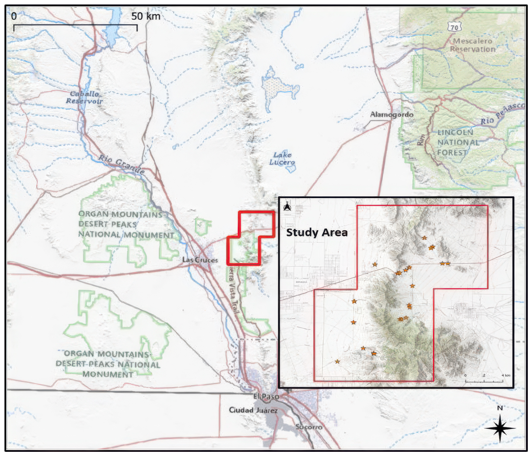
Our VBN evaluation of horizon matching used a desert location near the Organ Mountains in New Mexico (roughly centered at 32.331 N and 106.5554 W, elev. 1879 m) in the Chihuahuan Desert, approximately 20 km northeast of the City of Las Cruces (Figure 1).

The region is characterized by an arid to semi-arid (Steppe) climate and located near southern end of the Rio Grande Rift Valley. The study site was located near the San Augustin pass, separating the Organ Mountains to the south and the San Andres Mountains to the north [25]. Our justifications for using this region were that it offered largely unobstructed features at ranges of greater than 1 km and challenged the ability of the algorithm and phone-based workflow for multiple stand-off observations. In the future, it is our intent to investigate other physiographic regions as funding becomes available. Two polygons, a northern (14 km by 11 km), and a southern (13 km by 12 km) were established as the AOIs and contained a rich variety of near- and far-field terrain features (50 m to >1000 m) that served as ground imagery reference points for the VBN database and positional solution. Using the Las Cruces Municipal meteorological report for 13 June 2024, the meteorological surface observation recorded a northern surface wind direction at a velocity of 3.1 m s⁻¹, an unlimited cloud ceiling (coded as 22,000 m), and a horizontal prevailing visibility of 16,093 m (10 statute miles), occurring alongside an ambient air temperature of 26.0 °C and a corresponding dew point temperature of 3.6 °C.

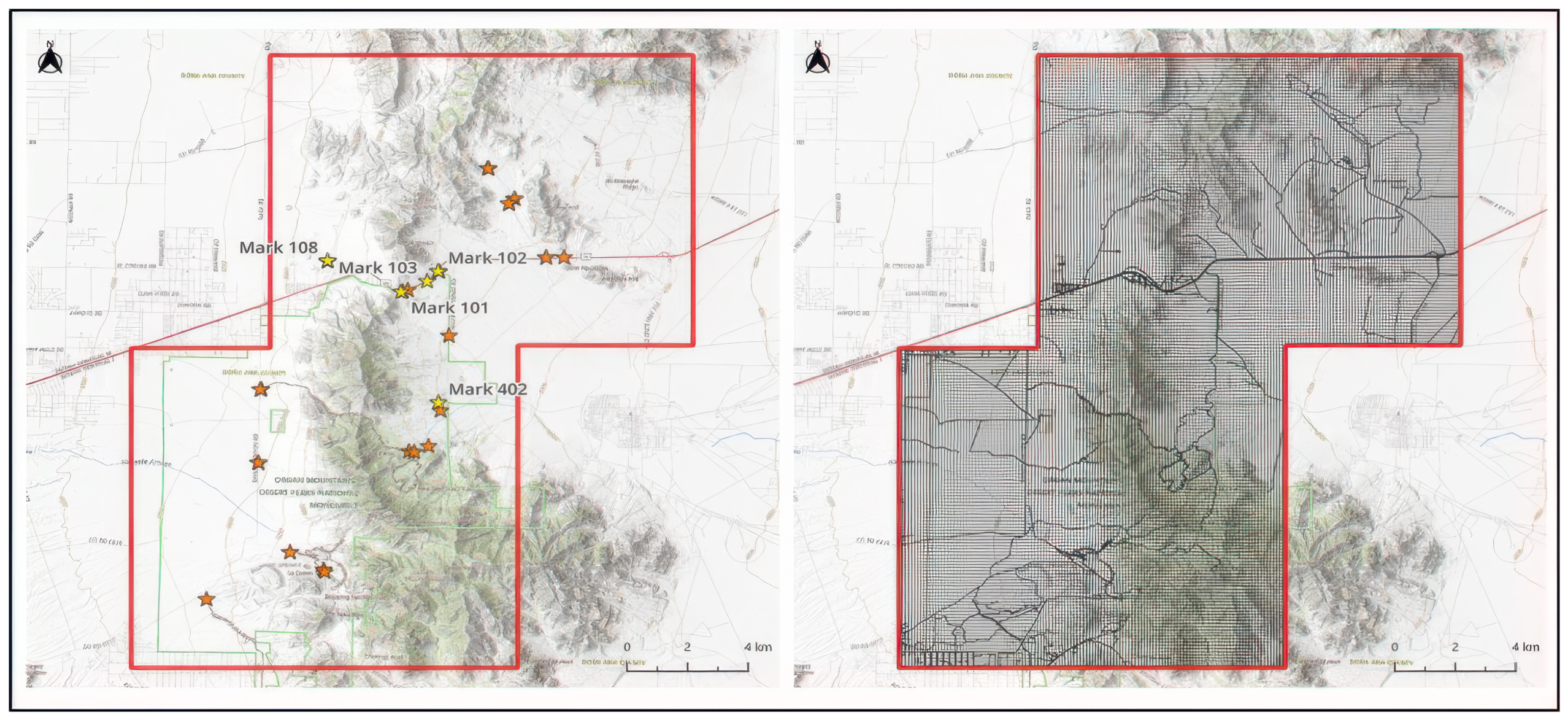
The testing scheme involved the use of the Samsung S23U cellular phone and main camera. The S23U camera hardware is shown in

Table 1. Features of the Samsung S23U camera used in the evaluation (https://www.samsungmobilepress.com (accessed on 29 June 2025)).

S23U Feature	Main Camera	Ultra-Wide Camera	Telephoto Camera
Resolution	200 megapixel	12 megapixel	10 megapixel
Pixel Pitch	0.6 µm	1.4 µm	1.12 µm
Aperture	f/1.7	f/2.2	f/2.4
Focal Length	24 mm	13 mm	70 mm
Sensor Size	1/1.3 in	1/2.55 in	1/3.52 in

[26]. Included on the S23U was the Android Team Awareness Kit (ATAK version 5.1.0.24 and our P3R plug-in v.2.1) and a pre-processed, 2.2 GB Geopackage containing the synthetic horizon profiles from the northern region seen above, with locations generated from a foundational, parent 3D terrain elevation databases [27]. In the initial step of our evaluation, a database of synthetic horizons was extracted by combining first, a regular grid at 100 m post spacing and second, a collection of posts spaced at 20 m along all the roads in the study area (Figure 2).

Grid size was selected based upon our experience with previous regions having open and long-range horizon features. This is not a restricted value, and we are evaluating this variable for other terrain scenarios. These roads originated from the OpenStreetMap “Highway” data set (https://www.openstreetmap.org, accessed on 24 May 2024).

The synthetic horizons for each post were generated using a modified version of the ray-tracing processing package “Horayzon” [28]. Our version of Horayzon (v1.2), Göttingen, DEU uses hardware-based ray tracing to calculate the elevation angle at each bin/post in the database and is specifically designed to compute topographic horizons and sky view factors (SVF) from digital elevation models (DEMs). For our data, this resulted in a gridded data set containing 31,389 posts, and the road-based data set contained 18,360 points for a total of 49,749 posts, where each 360° horizon was divided into 570 equally spaced bins.

2.1. Pre-Processing Synthetic Horizon Database

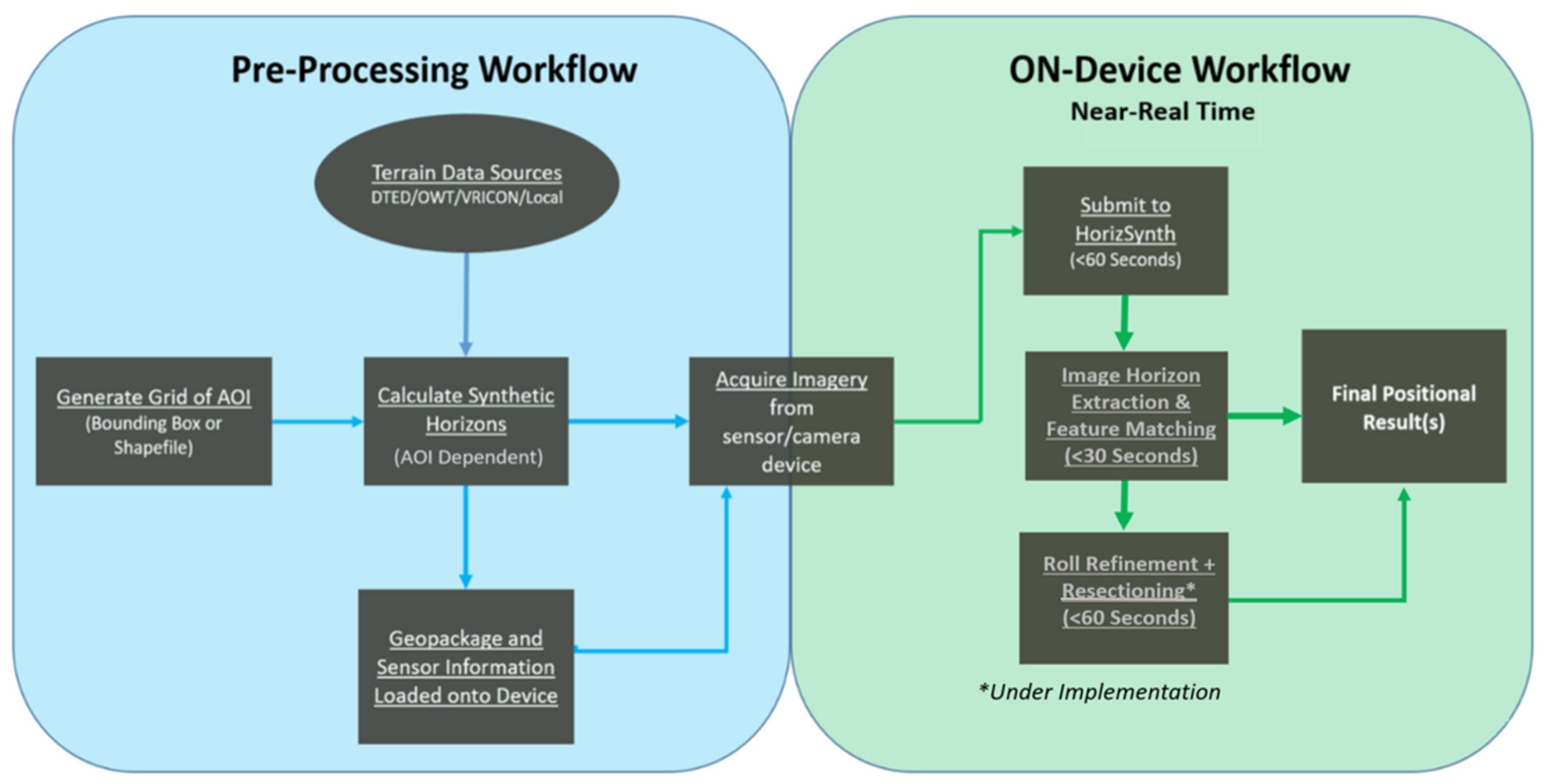
The pre-processing workflow involved (1) selecting a reference 3D terrain data source, (2) bounding an AOI, (3) grid generation resulting in a polygon (or bounding box) and a 360° viewshed computed for each grid point, (3) synthetic horizon extraction and database (Geopackage) construction, and (4) sensor optical information. Once these data are pre-loaded on the phone, the on-device geopositioning workflow can be executed as shown in Figure 3. The terrain data sources used in our evaluation were the following two data sets acquired in 2021: Maxar (MAXAR Space Systems, Palo Alto, CA, USA) with a ground sample distance (GSD) of 50 cm/pixel and vertical accuracy of <3 m (LE90—Linear Error 90%) and a TanDEM-X (European Space Agency) possessing a GSD of 12 m and vertical accuracy of <4 m (LE90). For this experiment, we selected a 100 m open-grid area and 20 m road spacing to optimize horizon generation and processing performance based on the coverage area of the test and GSD of the data set. Other sources of elevation data (high-resolution airborne lidar, terrain data processed from drone imagery, etc.) may also be used if they are available to the pre-processing stage and are in the same horizontal and vertical map datum. The two data sets were combined using the open-source, command line Geospatial Data Abstraction Layer (GDAL) virtual raster data set (VRT) tool.

A series of reduced resolution images, acquired and processed at each camera station location or “Mark”, were created from the VRT data set based on the S23U’s main camera focal length and pixel resolution. These same parameters correspondingly determine the number of “bins” (n) into which the 360-degree horizon is divided. The final output of processing is a set of vectors representing the horizon at each camera (observer) station. Each observer station has one n x 1 vector representing the horizon as elevation angles.

2.2. Collected Camera Images and Horizon Quality Analysis

After completion of the synthetic horizon database, camera images can be acquired. For effective derivation of a sky/non-sky horizons in imagery, an objective computational analytical technique was used to allow for quality assessment and further vision-based localization from that horizon. This approach was used to evaluate the horizon generated from the techniques described in Section 2.4 below. For many edge-detection algorithms, the gradient is a useful operator to determine a true boundary between image segments [29]. For two dimensions, such as with an image, the gradient ($\nabla F$) is defined as the following:

$$\nabla F={\displaystyle \frac{\partial F}{\partial x}}\widehat{I}+{\displaystyle \frac{\partial F}{\partial y}}\widehat{J}$$

(1)

where in this case the x direction could be columns and the y direction rows. However, where we already have a defined horizon, we are only interested in the gradient above and below that horizon intersection point for each column. In this situation, the gradient in one dimension simply becomes the central difference, which for an intensity image I in the vertical direction ($\partial y$) would be the following:

$${\displaystyle \frac{\partial I}{\partial y}}={\displaystyle \frac{\left(I\left(y+1\right)-I\left(y-1\right)\right)}{2}}$$

(2)

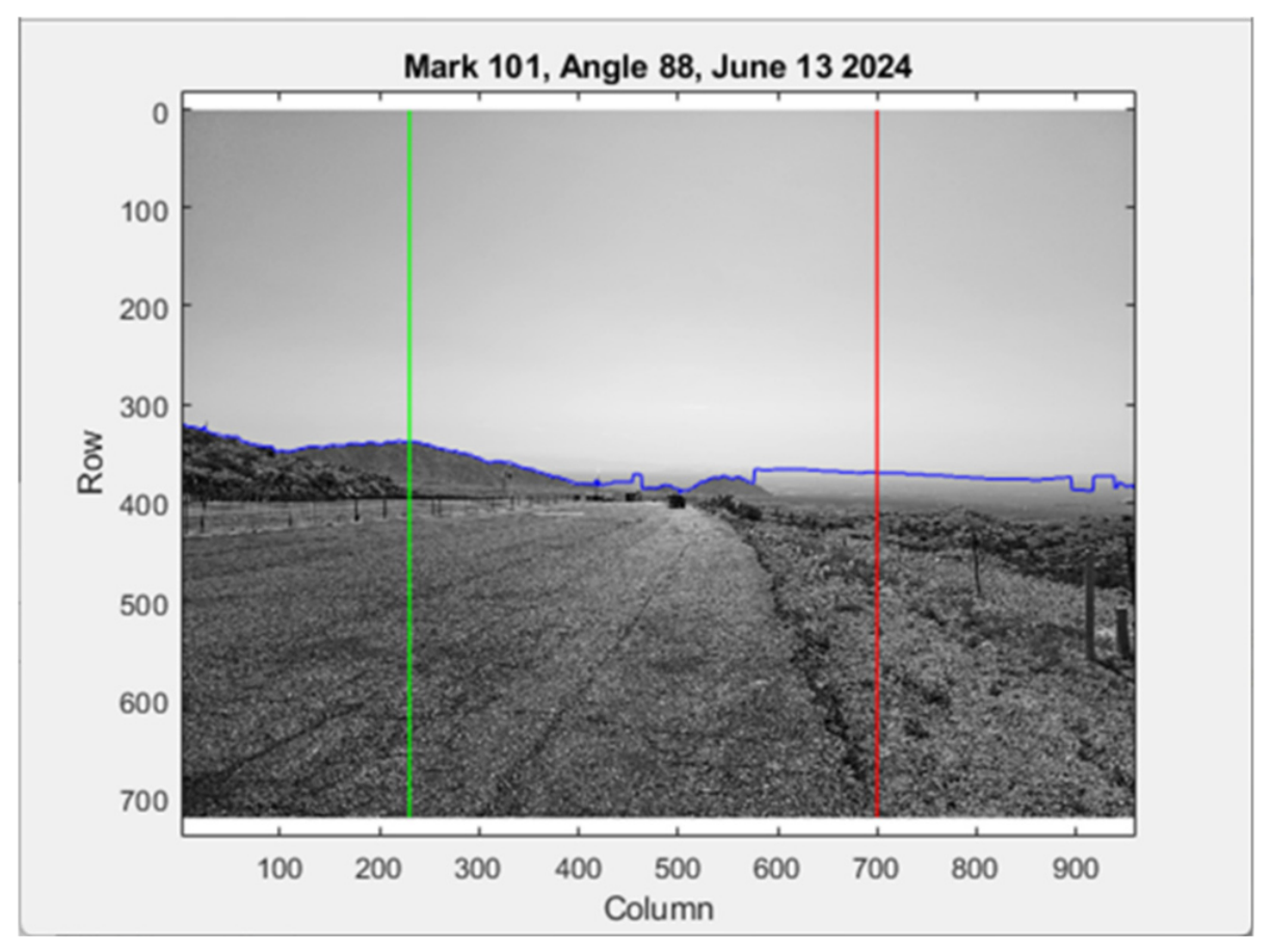
For the Organ Mountain environment, the sky pixels (above the horizon) are more homogeneous than the non-sky pixels (below the horizon). So, for each column the gradient values above the horizon should be smaller (close to zero) than below the horizon. Two examples are shown below depicting how the gradient information was used to assess image quality for vision-based localization. The first example is from camera Mark 101 and shows the impact of distance haze on the extracted horizon (Figure 4).

For this example, the RGB image has been converted to intensity (or luminance) via the following formula [30]:

$$I=0.299R+0.587G+0.114B$$

(3)

where R, G, and B are the red, green and blue pixel values from the Samsung S23U image. Green and red vertical lines are shown on this image to draw attention to the accuracy of sky/non-sky horizon line detected by the algorithm (blue line). The green line, which corresponds to column 230 in the image, intersects the horizon where there is good separation between the sky and non-sky pixels. The red line, which corresponds to column 700, intersects the “detected” horizon within a haze layer as the true terrain/sky horizon is too far in the distance to be detected in these conditions. This would be considered a poor separation between sky and non-sky pixels.

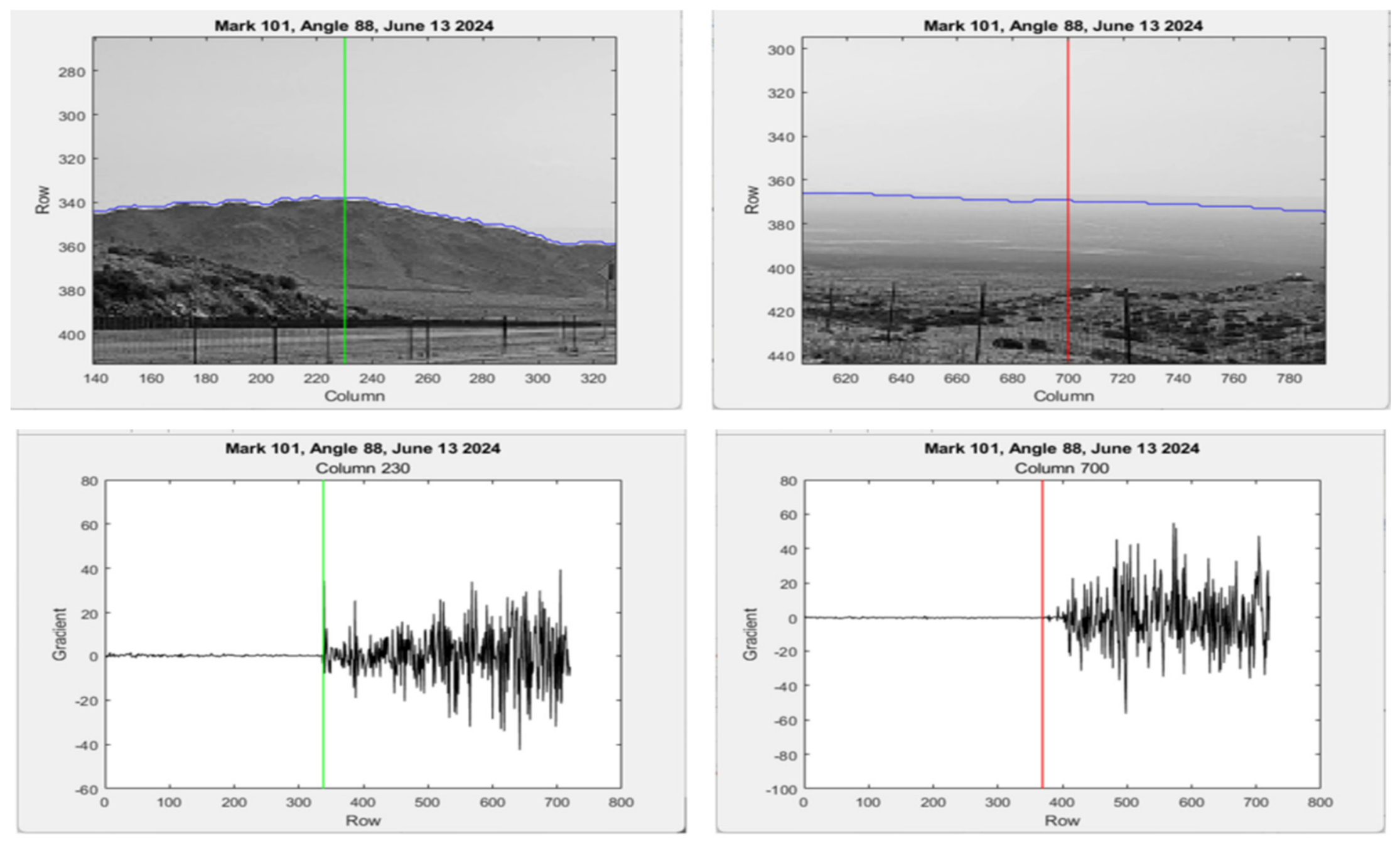
Figure 5’s compilation shows a close-up of where the green line (top left side) and red line (top right side) cross the detected horizon. As shown in Figure 4, the green line crosses the horizon at a true sky/non-sky interface, while the red line crosses the detected horizon in the haze layer. The bottom left and right graphs in Figure 5 show the gradient for columns 230 and 700, respectively. The left side shows that at the detected horizon (approximately row 342), there is a sharp change immediately after the horizon intersection, which provides confidence in a correct horizon detection. However, when analyzing the bottom right graph in Figure 5 (the haze intersection, about row 365), the gradients immediately before and after the detected horizon are similar, which shows a low confidence in a correct horizon detection. Similar to the need for a quality assessment where the haze is a substantial component of the horizon is a case where near-field objects result in horizon anomalies [31].

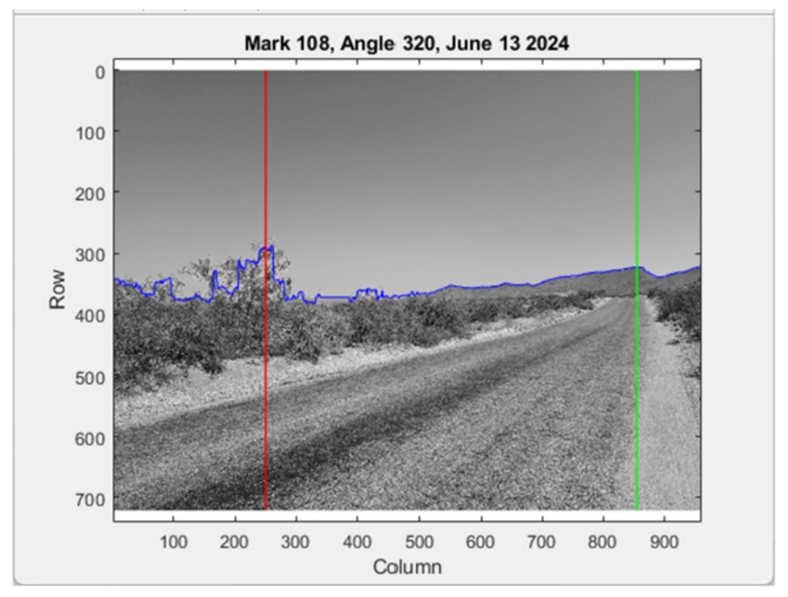
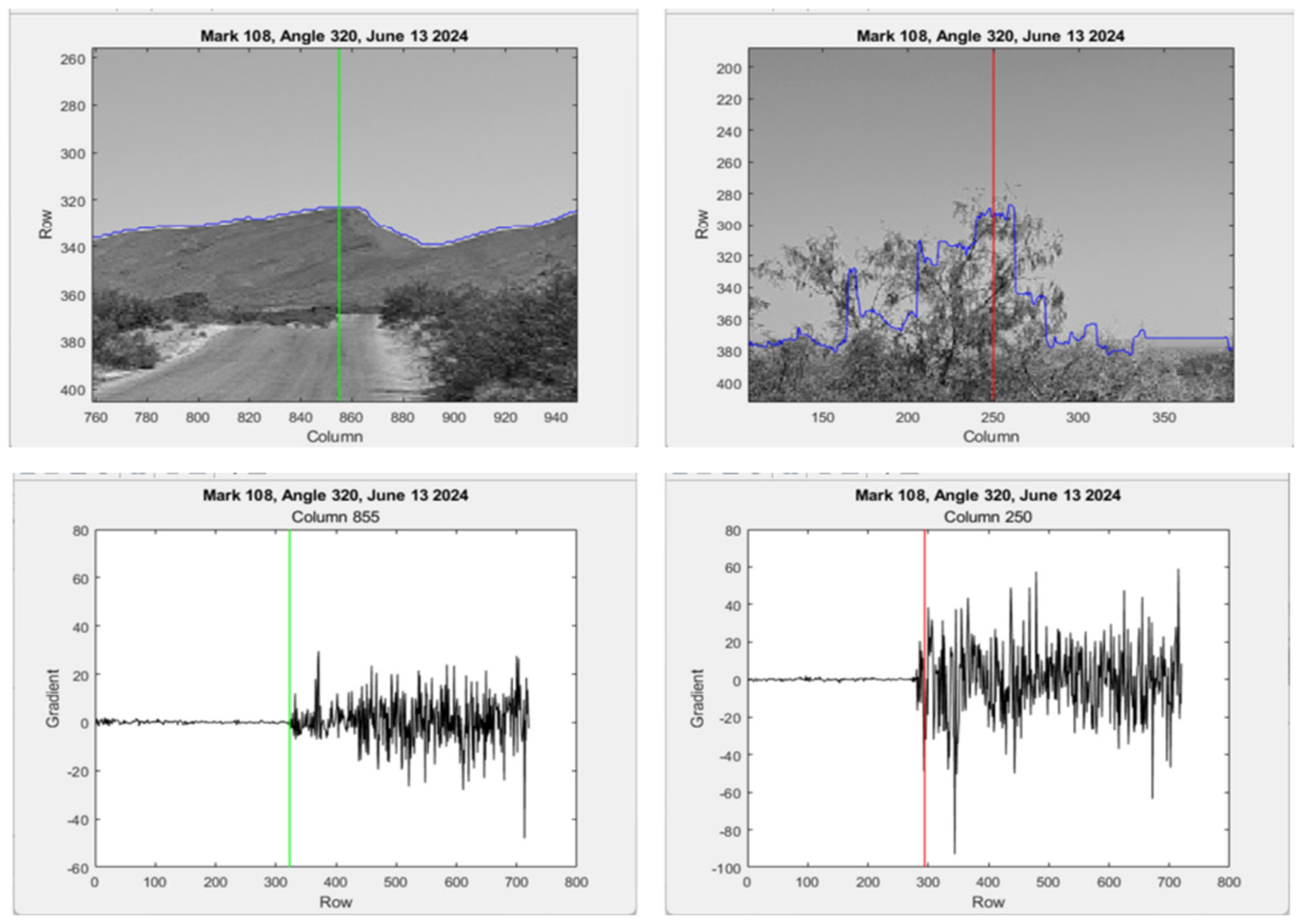
Figure 6 shows a different image from the Organ Mountain area. The image from Mark 108 at an azimuth of 320 degrees has near-field vegetation in the skyline that would not be resolved with most digital surface model data. As with the previous example, the green line, this time in column 855, intersects the detected horizon over a distance mountain. The red line in column 250, intersects the detected horizon over some near-range vegetation. The top two images presented in Figure 7 show a closer view of the intersection for both the green (left) and red (right) lines. The bottom two images in Figure 7 show the gradient values for the green and red line columns. The gradient data for the green line are as before; the gradient data are relatively flat from the sky pixels and then show image heterogeneity from the terrain pixels. The data for the red line, which intersects the vegetation, show gradient structure both above and below the detected horizon.

Extending this analysis to all columns for all images provides a numerical method to assess image quality. The mean of the absolute value of the gradient values is generated a few pixels (nominally 5–10) above and below the detected horizon line. Where the gradient values show a marked change at the detected horizon is considered a valid horizon point. Where there is little difference (either both flat—haze or both with structure—vertical obstruction) is considered a poor horizon point. Based on this analysis, we organized the 278 Organ Mountain images into three classes based upon the quality of the detected horizon as determined by the gradient method described above. An image with a detected horizon with less than 15% of the pixels showing haze or vertical obstructions was considered “high quality”. An image showing between 15% and 30% haze or vertical obstruction was considered “fair quality”. Finally, images with greater than 30% haze or vertical obstruction were considered “poor”. Statistically, this was represented in computing the descriptive statistics for the test images and using the “high-quality” images as the reference to explore the percentile error for the “fair and poor-quality” images.

Table 2. Image categories and descriptive statistics.

Image Quality	Mean	Standard Deviation	Percentile Error by Pixel
High (n = 18)	133.07	51.79	n/a
Fair (n = 8)	135.07	37.99	0.4991/4.92%
Poor (n = 6)	129.89	39.25	0.994/9.94%

shows these statistics and error by pixel count with the fair-quality images possessing 4.92% error compared to the high-quality-image data. The poor-quality data have a percentile error of 9.94% compared to the high-quality images. This increasing error in quality represents the quality and availability of horizon features to derive an accurate position once compared to the synthetic database.

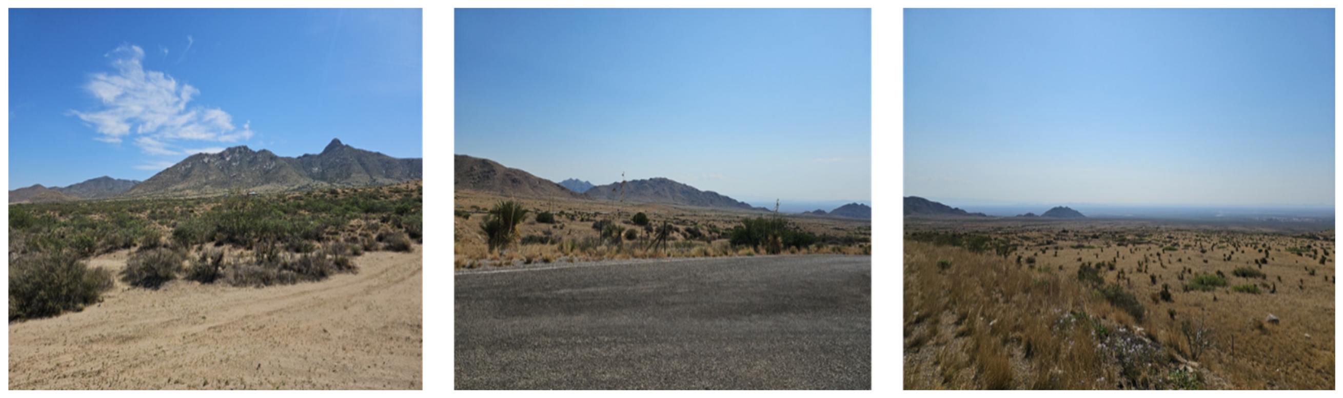
Our collection produced 278 images of varied quality and uneven distribution across the three categories for long stand-off feature matching from around the southern portion of the AOI. Our analysis permitted us to bin these images into three categories—high, fair, and poor—possessing identifiable features and known distance from the point of an observer (Figure 8). Based on previous processing, we expected high-quality images to have a clean, well-defined horizon producing good results (Figure 8—left). These features were typically within 10 km of the observer. Fair-quality image horizons are shown in Figure 8 (center) and have a mix of high-quality and poor-quality features where extraction and matching can be difficult. For example, the left two-thirds of the image show a good skyline, but the right-third has hazy, flat horizon features far in the distance. These images fall into a range of 10 to 20 km from the observer. Figure 8 (right) is an example of a poor image horizon with mostly flat features that are hard to distinguish from the sky. These horizons will produce poor results as they contain an ill-defined or non-descript horizon or a horizon blocked by near-field trees or other obstructions. Our experience has shown that images with a significant portion of the horizon very far in the distance (e.g., >25 km) produce poor positional results, often because our horizon detection algorithm has demonstrated inconsistencies at these very long ranges. Such horizons are very difficult to discern from the skyline and are typically flat with few discriminating features.

2.3. Image Distortion Evaluation

Distortion evaluation and correction is typically the first step in any photogrammetric processing. Typically, this involves capturing several images of a well-measured grid of points and performing a least squares adjustment to fit a radial/tangential distortion model such as the Brown’s model or others [32,33]. With cell phone cameras it is difficult to determine what internal processing the manufacturer does before rendering the final image and often with modern versions the radial distortion (largest contribution) has already been corrected [34,35]. We assessed the potential S23U distortion by imaging a black and white grid of squares using the standard S23U phone application with distortion correction turned on and off and collecting two images. To eliminate any movement of the camera, we mounted the device on a tripod and operated the camera remotely from a PC desktop. Using this method, we found only 1–2 pixels of distortion between the two 4000 × 3000 pixel images located at the extreme edges and corners of the frame, indicating there was little distortion in the native GeoCam camera application images produced by the S23U that would adversely affect our horizon extraction should it be used in image capture. As a final check, we used an OpenCV-base application (https://github.com/niconielsen32/CameraCalibration/tree/main, accessed 17 April 2024) to check distortion of the GeoCam images. We processed a set of black-and-white grid square images to develop a set of correction parameters and corrected a test image with these parameters, comparing it to the original image and, again, observed only 1–2 pixels of difference between the two. Based on the evaluation described above, we concluded that uncorrected images from TAK GeoCam were sufficient for use in our horizon-matching positioning workflow.

2.4. On-Device Geopositioning

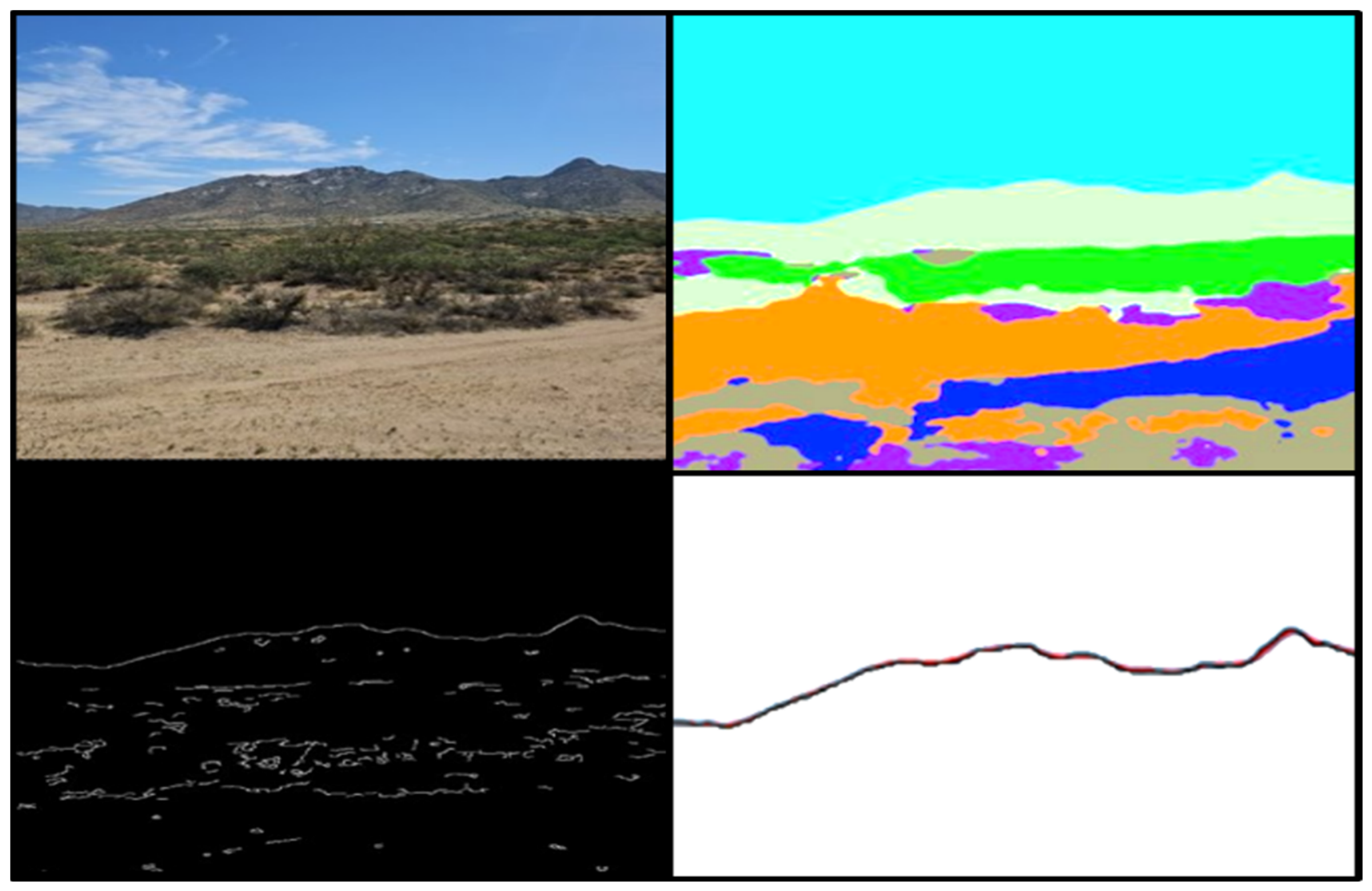
Horizon extraction on the S23U smartphone utilizes a sky detection method that incorporates a machine learning segmentation algorithm aided by an edge-detection algorithm. This workflow allows for the horizon to be extracted in near real time due to both algorithms’ less computationally-burdensome nature. Initially each image is run through a segmentation model that classifies pixels within the image. The resulting multi-class mask is then converted into a binary image with sky and non-sky classified pixels. This binary mask provides an initial, coarse horizon estimate. For each vertical column of pixels in the image, the algorithm identifies the lowest coordinate “sky” pixel. However, due to the required downscaling of the input image for the segmentation model and subsequent upscaling, this initial estimate tends to smooth over fine details of the true horizon line. Subsequently, the OpenCV Canny Edge Detection function refines the horizon profile by identifying the precise boundary between terrestrial objects and the sky. However, the canny edge detection is prone to misidentification of unwanted objects, like cloud edges. An example of the algorithmic pseudocode used for processing this phase of the workflow is shown below (Algorithm 1):

Algorithm 1 Edge Detection Pseudocode

//Define algorithm parameters canny_pixel_buffer = 15//Buffer around segmentation horizon //Main function for horizon detection FUNCTION Find_Horizon (image):     //Pre-process the image     downscaled_image = resize (image, model.size)//Downscale image for the model     segmentation_mask = model (downscaled_image)//Get segmentation mask     upscaled_mask = resize (segmentation_mask, image.size)//Upscale mask to original size     binary_mask = create_binary_mask (upscaled_mask, SKY_CLASS)//Create binary mask of sky and non-sky pixels     //Edge detection edges = canny_edge_detection (image)//Compute Canny edge detection     //Initialize the refined horizon     refined_horizon = empty_list_of_size (image.width)     //Process each column of the image     FOR i FROM 0 TO image.width-1:         //Get initial horizon estimate from the segmentation mask         sky_edge = find_lowest_sky_pixel(binary_mask [:, i])         //Define a window around the initial horizon estimate         y_min = sky_edge−canny_pixel_buffer         y_max = sky_edge + canny_pixel_buffer         //Find Canny edges within the window         canny_window = edges[y_min:y_max, i]         edge_locations_in_window = find_edge_locations (canny_window)         //Refine the horizon point         IF edge_locations_in_window is not empty:           //Convert window-relative locations to absolute image coordinates           absolute_edge_locations = edge_locations_in_window + y_min           //Find the edge closest to the original segmentation horizon           closest_edge_y = find_closest_edge (absolute_edge_locations, sky_edge)           refined_horizon [i] = closest_edge_y       ELSE:           //If no Canny edge is found, use the initial estimate           refined_horizon [i] = sky_edge       END IF       END FOR       RETURN refined_horizon END FUNCTION

Ranftl et al. describe the machine learning algorithm we applied as a simple semantic segmentation model using Dense Prediction Transformers [36]. An example of this processing is shown in Figure 9, where an initial estimate from segmentation is refined with canny edge detection [37]. This is where the two-step process provides a distinct advantage. Because the segmentation model classifies clouds as “sky”, the initial horizon estimate lies below any cloud cover. Consequently, the Canny edge detector’s search for the true horizon is constrained to a narrow window around this robust initial estimate, effectively preventing it from misidentifying cloud edges as the horizon. In essence, the segmentation provides a coarse but reliable guide, while the edge detector provides precision. Readers may note that the other, non-sky, segmented edges may be of value as features for localization. In fact, the exploitation of other classes of segmented edges to include vegetation, urban, man-made, and multiple terrain edges (valleys, drainage, and other features below the skyline) are under consideration for future evaluations of the workflow.

2.5. Image Pixel Horizon Coordinate Transformation Workflow

Prior to matching captured image horizons to the pre-processed synthetic horizon database, a coordinate transformation must be applied to place the image data into the same coordinate system as the synthetic data. The pre-processed synthetic horizon database described in Section 2.1 is stored on the S23U as azimuth-elevation angle pairs in a cylindrical coordinate system. Captured image horizons are extracted as pixel coordinates and need to be converted to cylindrical coordinates for the matching process and subsequent geo-positioning. Azimuth angles are regularly spaced in the synthetic horizons database and, as part of the metatdata, the TAK GeoCam stores camera roll (φ), pitch (θ), and azimuth (ψ). Along with these parameters, the focal length of the camera in pixels (f_px) is also known. We used NumPy (v.2.2.6) and the following steps for converting from pixel horizon to elevation horizon were developed, starting with the pixel horizon, (h(x), v(x)), where h(x) is the horizontal pixel index from the center of the image and v(x) is the extracted horizon in pixels above the center of the image, as follows:

• Rotate the pixel horizon data by roll angle, (φ), about the center of the image where “dot” is the NumPy dot product, as follows:

h_r(x), v_r(x) = [cos(φ) − sin(φ); sin(φ) cos(φ)] .dot([h(x) v(x)])

(4)

2.

Apply pitch correction by converting pitch angle, (θ), to a pixel count from the center of the image, as follows:

v_rp(x) = v_r(x) + f_px × tan(θ)

(5)

3.

Compute the horizontal cylindrical coordinate indices as described in [33], where β is the angular size given by one pixel β = tan⁻¹(1/f_px), as follows:

h_{r_cyl}(x) = f_px × tan(xβ)

(6)

4.

Compute cylindrical radius for computing elevation angle, as follows:

r_cyl = sqrt(h_{r_cyl}(x)² + f_px²)

(7)

5.

Compute the elevation angle, as follows:

v_ang(x) = tan⁻¹(v_rp(x), r_cyl)

(8)

6.

Compute the horizontal pixels angles, as follows:

h_ang(x) = atan⁻¹(h(x), f_px)

(9)

This effectively places the image horizon, (h_ang(x), v_ang(x)), in the same coordinate system as the stored synthetic horizon database and permits curve matching between the two data sets.

2.6. Curve Matching Between Corrected Image Horizons and Synthetic Horizon Features

Next, a horizon comparison routine based on Shen and Wang is performed that implements an error minimization and maximum correlation search that is used to determine the best-fit synthetic horizon from the database [38]. Mueen’s Algorithm for Similarity Search (MASS ver. 4) is used to find the find the best azimuth alignment between the image horizon and the database of synthetic horizons [39]. Once the horizons are aligned, a standard Pearson’s correlation coefficient is applied to find the synthetic horizon with the best match to the image horizon.

Once the image horizon is placed into the cylindrical synthetic database coordinate system, we can execute the curve matching process and begin the geo-location process. The image horizon, h_ang(x), v_ang(x), is irregularly space along h_ang(x). To curve match against the database, we need to interpolate into the regularly spaced values of the database, h_db(x) given that

v_{ang_db}(x) = interp(h_db(x), h_ang(x), v_ang(x))

(10)

where interp is the NumPy standard 1D interpolation function (https://numpy.org/doc/stable/reference/generated/numpy.interp.html, accessed 20 May 2025). After interpolation, we apply the azimuth (ψ) from TAK GeoCam to get the final horizontal indices, h_f(x) for searching the synthetic horizon database:

h_f(x) = h_db(x) + ψ

(11)

For each grid post in the synthetic horizon database the following steps are computed:

• Use “findNN” (https://www.cs.unm.edu/~mueen/findNN.html (accessed 20 May 2025)) from Mueen’s Algorithm for Similarity Search (MASS) to find the distance between v_{ang_db}(x) and all locations along database signature, v_db, where d = findnn(v_{ang_db}, v_db).
• This index of the minimum value of d gives us the azimuth offset between h_f(x) and the best match for the current grid post.
• Shift the h_f(x) to the best match in the current post: h_fd(x) = h_f(x) + index[min(d)].
• Compute Pearson’s correlation coefficient between the curve and the corresponding section of the curve from the synthetic database, v_db: cc(post) = corrcoef(v_{ang_db}, v_db) where corrcoef is the standard NumPy corrcoef function (https://numpy.org/doc/stable/reference/generated/numpy.corrcoef.html, accessed 20 May 2025).
• Repeat steps 1–4 for each post in the database.

The post with the highest correlation coefficient is the best match for the image curve. Its location is our final estimated geographic position. As part of the point extraction, horizon-matching and roll-processing workflows, critical camera information that accurately defines sensor optical characteristics (e.g., focal length, pixel pitch, and field-of-view) is also utilized. Once extracted, the resulting values are ranked and weighted to refine the estimated position and orientation. For improved accuracy, simultaneous sensor images can be collected at varying orientations by the camera to afford a more robust geolocation solution. For this study, we used the EXIF position metadata served as “truth” recorded at the time of the image capture that uses the internal GPS receiver, phone accelerometer and gyroscope for localization. In a recent study, Ryser et al. report in open-sky areas, EXIF generally provides 2 to 13 m accuracies [40]. We, therefore, computed the relative accuracy by using the distance between the EXIF and image horizon-matched positions.

3. Results

3.1. Horizon Extraction Processing—Single-Image Solutions

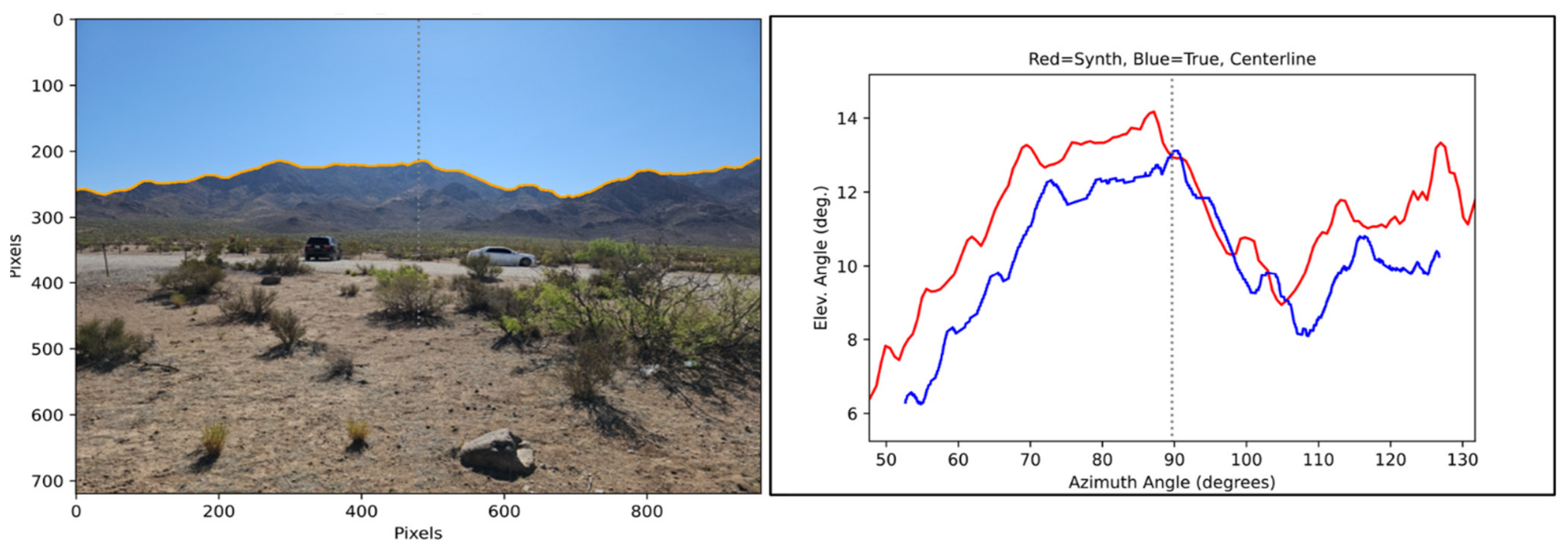
Figure 10 (left) shows a sample single image collected at the Mark 103 position with its extracted horizon (orange trace) and a vertical, dashed image centerline for reference. This image was collected west of the center of the study site at Long. −106.651702, Lat. 32.346759. Figure 10 (right) shows a plot of the extracted horizon (blue) and the synthetic horizon (red) of the post in the database closest to EXIF position of the image and includes the peak at the vertical centerline. The closest posting is indicated by the dashed line near the image center for illustration and reference. This figure shows the true horizon (blue) plotted at the azimuth (89.8°) as recorded during image acquisition by TAK GeoCam and saved in the EXIF data. From this analyses, there is an error of about six degrees in the EXIF azimuth.

This figure also shows the reference centerline in the middle of the plot. The closest post is about 22.6 m. away from the EXIF (truth) position.

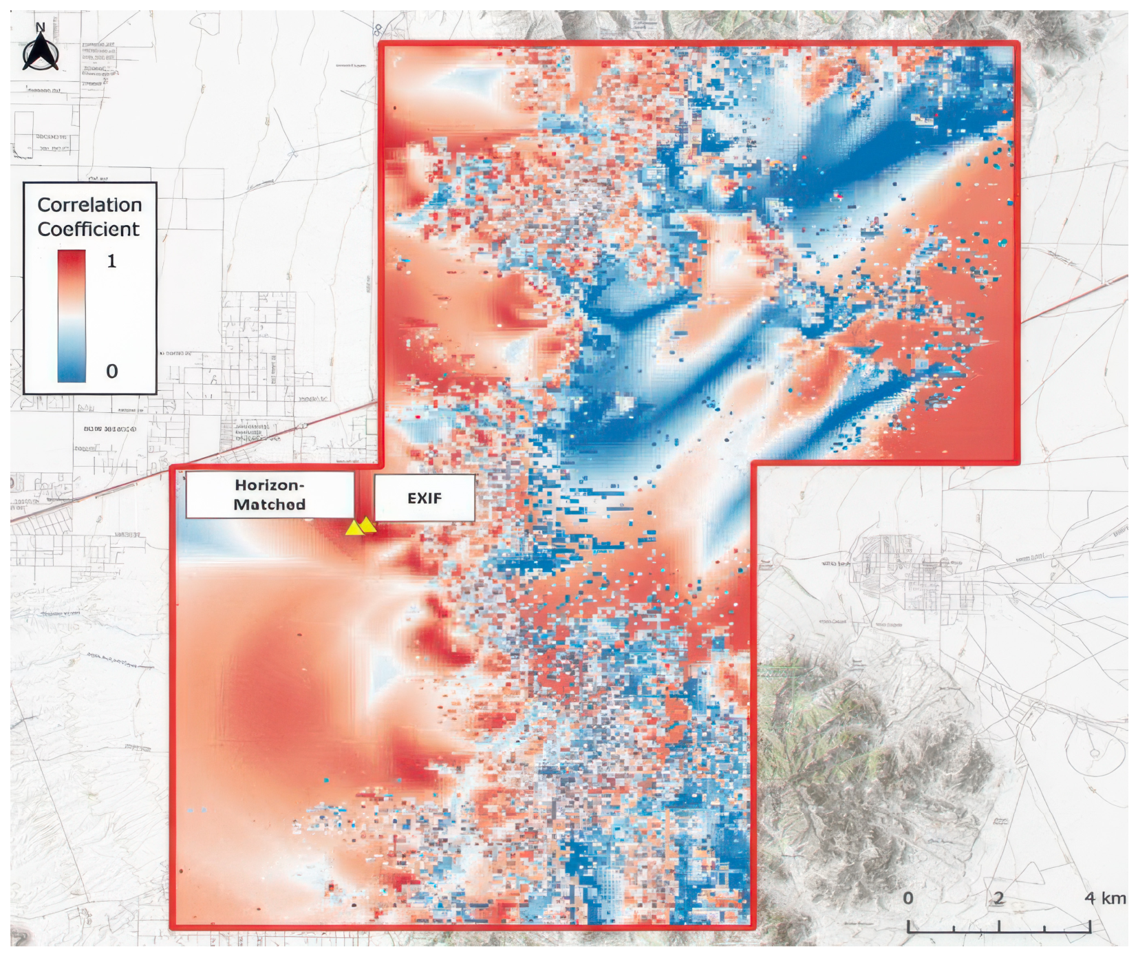
The results from individual directional image runs were overlaid and averaged to find hotspots in correlation values (Figure 11). We applied weighted average based on the attributes in the data set to construct a heat map representing position correlation coefficients within the QGIS (ver 3.44 Solothurn) geospatial package. Visually, a heat map generated for the solutions from the Mark 103 image is presented with darker reds representing areas of higher correlation (closer to 1.0) and darker blues representing areas of lower correlation (closer to 0.0). The graphic also shows the EXIF position and estimated horizon-matched position, that are very close at this scale. These positions are in within the brightest red section (highest correlation coefficient) on the heat map. This workflow increases the computational time dependency on the number of images collected but improves overall accuracy in locations where a single image fails to extract distinct matching features in one direction.

3.2. Comparing Image Quality and Azimuth Correction Application

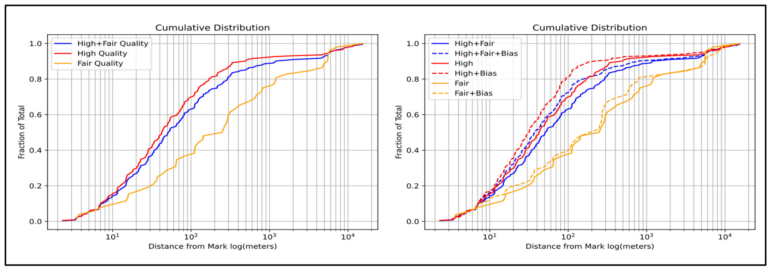
As mentioned, accuracy was determined by computing the distance between the image EXIF position and horizon-matched-computed position. Figure 12 shows the results for our single images as collected. The graphic shows the cumulative distribution of distances from truth (EXIF) for the high-quality images, the fair-quality images, and the high- and fair-quality images combined. The blue line shows results for the high- + fair-quality images. About 14% of the solutions were within 10 m of the actual position, 49% were within 50 m, 63% were within 100 m and 75% were within 200 m. As expected, the high-quality images alone have better results (red curve, 75% within 100 m) and the fair-quality images alone have worse results (orange curve, 38% within 100 m).

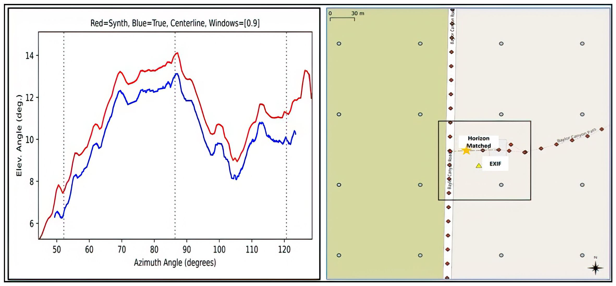
While our evaluation was chiefly focused on single- and multi-image-derived solutions, our analysis of all 278 images showed an average roll-bias on −0.73 degrees. As applied here, a roll-bias correction is intended to show the potential improvement as part of a future field-calibration procedure applied to all affected images solutions. The process we are developing involves computing the average bias (from all 278) images over known locations and the results presented in Figure 13 showing the potential benefit of such an appropriate and robust procedure that is not presently practicable for field implementation. We attempted to quantify this roll-bias by aligning each of the high-quality images with its closest post from the database. We estimated the roll error for each image by implementing a linear fit of the differences between the two curves. An overall bias was computed by averaging all the roll errors for all the high-quality images. Figure 13 (left) shows data from the Mark 103 image collection position. The original cumulative distributions (solid lines) are compared to the roll-bias corrected images, cumulative distributions (dashed lines) and the subsequent improvements for each image type where between 9% and 13% were achieved. Figure 13 (right) shows final alignment of the position as calculated by horizon matching using the MASS algorithm to find the best azimuth for each post; then Pearson’s correlation coefficient was calculated between the two. The estimated position (star icon) comes from the location of the post with the highest correlation coefficient. In this case, the estimated position was 26.5 m away from the EXIF (triangle) position. For this testing, we used the center 90% of the image horizon to calculate Pearson’s correlation coefficient. With the current lack of such a practical procedure, we are offering most of our results without any bias correction to provide a candid representation of what a user could potentially expect from the basic workflow. Although the results reported here were not corrected for roll-bias, we hope to implement a bias correction after more testing and evaluation that may be applied to data possessing such issues.

3.3. Horizon Extraction Processing—Multi-Image Solutions

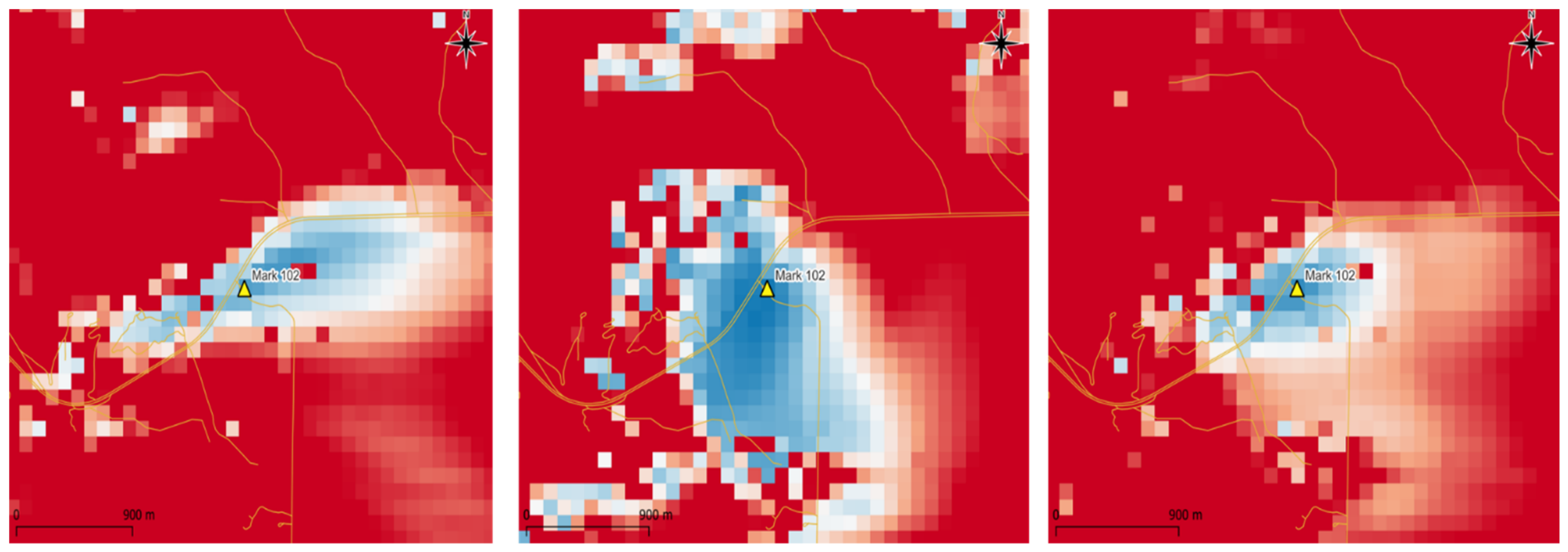
From an operational perspective, there is no reason an observer should be constrained to collect only single images. In fact, in practice, we have found it intuitive to take multiple images at different azimuths, standing stationary at an observation Mark. Conceptually, the exploitation of multiple images should improve positional accuracy with the introduction of varied terrain perspectives within a field of view. In practice, the collection of multiple images is useful with data sets that have a high number of strong matching correlations near the true position. This is the often the case where prominent features are observed from longer distances such as was found with the Organ Mountain data. In our example, slight translations from the correct position when observing the Organ Mountains from a distance will still produce high correlations. This results in “hot spots” that were described in the previous sections using heat maps to show areas of correlation. When exploiting multiple images, these hotspots can be combined by computing and averaging the heat maps from each image. Our process isolates consistent spatial clusters across all image results and produces a highly robust estimate of the true location while mitigating single-image false positives and in many instances produce an improved position solution. Images acquired from the same location were shown to improve the accuracy of positions, even from fair and poor categories of images. As an example, Figure 14 shows the results from individual and combined positional determinations as a series of heat map estimates from camera station Mark 102, a data set possessing poor image qualities as determined by the described method in Section 2.2. This multi-image solution estimate features two image results from two different azimuths, 325° (Northwest) and 225° (Southwest) with the size of the blue area around the point indicating higher accuracy the smaller the area becomes. In this case, the far right image (a combination solution of the two images) shows a tighter blue area which corresponds to a more accurate estimate of position. The individual scenes show prominent hot spots where the centers are not at the exact correct position. However, the raster combination of the two images produces a reduced hotspot with the center/highest raster correlation closer to the true position (11 m).

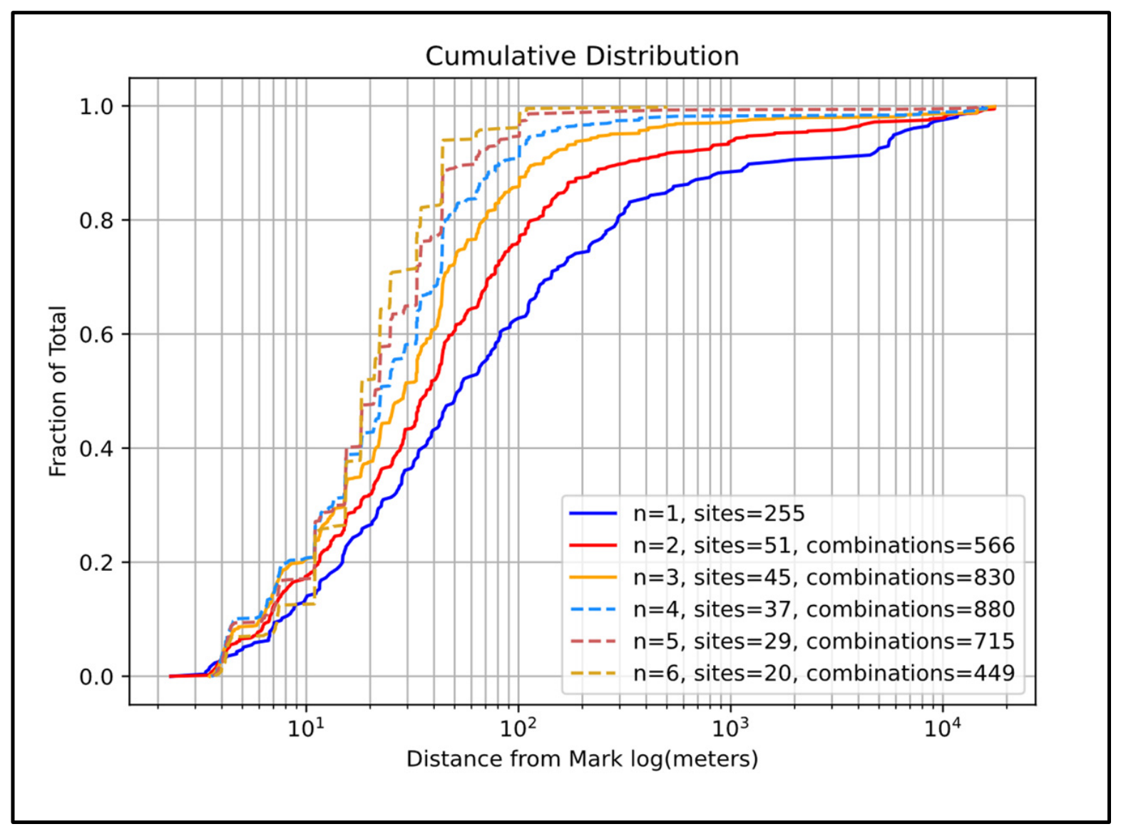
There were 51 separate sites from the 255 high + fair images. (locations with images within 2 m of each other). From these 51 sites, there were 566 unique combinations (combos) of two images. There were 45 sites with three or more images and 910 unique combinations. Figure 15 shows the cumulative distribution for the original high + fair results (without bias correction) and results for the two through six combinations of images. The high + fair percentage of solutions within 100 m of the mark improved from 63% to 76%; three images improved to 85%; four images, 90%; five images, 95%; and six images, 97%.

Collectively,

Table 3. Single- and multi-image accuracies derived using the S23U imagery and horizon matching, positions in meters, UTM Zone 13.

Observation Mark	Image Quality	EXIF (Image) Position	Horizon-Computed Position	2D Distance (m)
103A	High	353,695.7 E, 3,589,029.1 N	353,710.0 E, 3,589,049.8 N	25.1
103B	High	353,695.3 E, 3,589,029.3 N	353,610.0 E, 3,588,995.2 N	91.0
103C (Multi-Image)	High + High	353,695.5 E, 3,589,029.2 N	353,675.8 E, 3,589,028.8 N	19.7
402A	Fair	354,066.9 E, 3,584,431.0 N	355,700.0 E, 3,596,000.0 N	11,683.7
402B	Fair	354,068.8 E, 3,584,430.0 N	354,700.0 E, 3,584,300.0 N	644.4
402C (Multi-Image)	Fair + Fair	354,067.9 E, 3,584,430.5 N	354,200.0 E, 3,584,300.0 N	50.3
102A	Poor	354.059.4 E, 3,589,408.3 N	350,500.0 E, 3,592,900.0 N	4986.1
102B	Poor	354,059.6 E, 3,589,408.0 N	357,200.0 E, 3,590,200,0 N	33,238.8
102C (Multi-Image)	Poor + Poor	354,059.5 E, 3,589,408.1 N	353,300.0 E, 3,590,600.0 N	1413.3

shows the results for representative images across the determined image qualities, their EXIF and horizon-computed positions in UTM coordinates and the final computed 2D distance result for the vision-based positions as determined by horizon matching (e.g., Easting—X and Northing—Y directions). The high-quality images yielded the best results, with multiple images in each category greatly improving the positional accuracy of each evaluated observation. In multi-image processing, we compute results by averaging Pearson’s correlation coefficient for each observation post in the database. This can (but not always) be used to mitigate errors from single-image processing.

Table 3 illustrates these results more clearly. For Mark 103 from Table 3, both single images have good individual results (25.1 m, 91.0 m). The average result for Mark 103 is slightly better (19.7 m) than the best individual result (103 A, 25.1 m). For Mark 402 each individual image has an outlier result far from the actual location (11,683.7 m, 644.4 m), but the average result has a good result (50.3 m). Averaging the results from multiple images has mitigated the outlier results from the two individual images. This does not happen in every case, but this example shows the benefit of using multiple images. Mark 102 has poor results for both input images (4986.1 m, 33,238.8 m). The average result is still poor (1413.3 m) showing that averaging does not necessarily work well in every single case. Although additional testing is needed in more complex and challenging feature environments, our evaluation shows encouraging results for determining position using only the computational horsepower of a cell phone.

3.4. Processing Observations

Execution of each stage using the S23U processor has been explored, and we show in

Table 4. Processing demand information for the S23U.

Area of Interest	Database Size (On Device)	Pre-Processing Time	Areal of Interest Coverage (AOI)	Processing Time to Position—Single Image	CPU Device Load S23U
Urban- Short-Range Horizons	238 MB	40 Seconds on Linux	3.84 sq km	14 s initial run, 7 s subsequent runs	551% CPU of 800% Possible
Desert- Long-Range Horizons	222 MB	38 Seconds on Linux	3.09 sq km	13 s initial run, 7 s subsequent runs	493% CPU of 800% Possible

the following two disparate data sets: an urban data set possessing complex short-range horizons and the desert data set featured here with long-range horizon features. For the ATAK and P3R plug-in, processing the two data sets on the S23U each data set possessed a similar size. At start up, 1.2 GB was required and memory space allocation stayed within pre-allocated levels (with an 8 GB physical limit). The standard operational state for the S23U CPU (central processing unit) is around 460 MB. This allowed the efficient and fast processing of a single-image position derivation to be recorded at 14 to 13 s for a 238 MB and 222 MB scene, respectively. We believe this performance can be greatly improved with faster processor capability and new compression algorithms that are currently being explored.

4. Discussion

To evaluate the ability for a common smart-phone camera system to determine its position without GPS, experiments were conducted with a Samsung S23U smart phone to match image horizons to a synthetic data set generated from foundation surface models. The 278 images collected over the Organ Mountain site were analytically binned into three quality classes. As reported, with a pre-processed database of synthetic horizons generated at a 100 m grid spacing combined with 20 m road spacing where only one high-quality ground photo was acquired, 75% of solutions were within 100 m. Single images of fair quality resulted in positional accuracies within 100 m in only 38% of the solutions. Not surprising, multiple images collected and processed from the same location produced correspondingly better positional results as observed in other studies and experiences in autonomy and robotics vision [41]. Importantly, accuracy in vision-based positioning are dependent on many associated factors observed in the literature including post spacing in the database, as well as image quality [42,43]. For example, we presented results within 100 m as “good” in the paper because the database utilized a 100 m grid spacing. In our assessment thus far, we observed that for a 100 m × 100 m grid, a random point, on average, would have a positional solution of about 37.5 m from the nearest post. Given this, a thorough examination should be conducted with regard to post-spacing influence, as well as the influence of image resolution on a solution accuracy using both single- and multiple-image collections and processing.

As work continues to evolve, the overall function and applicability of this approach to other and more complex environments, multiple discussion and improvement areas have been noted. First and foremost is the need to investigate other analytical tools that evaluate the “quality” of the image to be used to extract the image-based horizon. Our 1D and 2D gradient analysis technique allowed for quantitative assessment of an image horizon based upon one sound approach in the literature. This allowed for three broad classes (“high”, “fair”, and “poor”) to be categorized based upon the quantitative metric of heterogeneity between sky and terrain (pixels), indicating where the segmentation algorithms will perform well. “High” images had substantial identifiable horizon features and contrast between the sky and non-sky, “poor” images were analyzed to have mainly flat horizons and sub-optimal sky/non-sky contrast, and “fair” images were somewhere in between. Future versions of this application will attempt to quantify classification by integrating other approaches that will analyze the shape of the profile as well as the radiometric characteristics of the images including adding a metric for applying procedures for evaluating line feature strength to images to gage feature clarity, edge density and gradient magnitude (or average intensity) of detected edges and an improved Sobel operator for checking line features [44,45].

A second area of improvement mentioned was a more robust integration and understanding of a multi-image approach. From an operational concept, collecting multiple images at the same location is quite simple: collect a picture, rotate in an azimuthal direction, and take another. In this instance, a roll-bias correction would be advantageous as part of the permanent workflow. The only real concern could be data storage and computational load. However, these would likely be mitigated under most normal circumstances. Images could be deleted soon after use, and a few extra seconds or even a minute or two for processing would likely be a small price for an individual in need of their location. Further work in the space could include improved analysis of multiple heat maps such as shown in Figure 11 and Figure 14. A weighting approach that could be considered is using an analytical quality metric noted above in a multi-image scenario. Another method would be to create panoramic signatures that would produce horizons that subtend more of the 0–360 azimuth range and, thus, could provide a more accurate result with a reduced computational penalty.

An additional mensuration technique that was only briefly mentioned and is under development for inclusion and testing into future versions of the workflow is the (spatial) resection method adaptive photogrammetric processing across variable feature environments [46,47]. As applied to terrain point features, this would be a valuable way to enhance image feature-based positional accuracy.

5. Conclusions

In this paper, we studied the ability of imagery collected from a commercial smartphone camera to generate a geographic position using vision-based localization techniques. The approach used a correlation method to match the sky/non-sky horizon extracted from the smartphone image to a synthetic profile previously generated from Maxar (50 cm) and Terra-SAR-X (10 m) digital surface models. A Samsung S23U smartphone was used to collect the imagery over multiple areas in the Organ Mountain region near Las Cruces, NM. This effort purposefully used a terrain site that was optimized to study the processing capability of positional determination using a cell-phone processor. The area provided a good variety of unobscured ranges and features for which to test each stage of the workflow to ascertain a cell-phone-based positional capability. The 278 images collected were analyzed and categorized into three quality classes (high, fair, and poor) describing the identifiable terrain features and their skyline horizon profiles compared to a geodatabase containing the synthetic profiles generated at 100 m grid-spacing using the Horayzon open-source-software method.

For the images judged to be of high-quality, 75% of the horizon-matched positions were within 100 m. For the images judged to be fair-quality, only 38% of those generated positions were within 100 m (the overall percentage of both high- and fair- quality frames less than 100 m was 63%). Additional analysis revealed that the roll of the smartphone during acquisition was impacting correlation between the image and synthetic horizons and adversely impacted the accuracy of the horizon generated positions. Through application of a roll-compensation method, accuracy of the horizon generated positions improved to 82% and 40% for the high- and fair-image quality data respectively.

A final analysis was conducted on the combination of images as opposed to the use of only single images, as in practice, it would be intuitive for a user to take images of multiple features while standing at the same point but changing their viewing azimuth. The results showed that by using both high- and fair-quality images, positional accuracy obtained through the horizon-matching process that were less than 100 m were 76%, 85%, 90%, 95%, and 97% for combinations of two, three, four, five, and six images, respectively.

To better understand the general functionality of the horizon-matching technique, the algorithm should be tested in multiple terrain environments. The Organ Mountain S23U data explored here was in some ways an optimal data set. The horizons produced by the sharp mountain peaks with an arid environment provided both structural features for correlation as well as high contrast between the sky and non-sky components. This is unlikely to be the case in other environments to include agriculture and forested areas where skylines may be less feature rich and the radiometric contrast reduced. However, with the maturing processing pipeline, horizon-matching algorithms can quickly produce results, whether or not an accurate position is generated. Understanding where, or where not, a particular algorithm will be successful is valuable knowledge.

References

1. Zidan, J.; Adegoke, E.; Kampert, E.; Birrell, S.; Higgins, M. GNSS Vulnerabilities and Existing Solutions: A Review of the Literature. IEEE Access 2022, 9, 153960–153976. [Google Scholar] [CrossRef]
2. Broumandan, A.; Jafarnia, J.; Lachapelle, G. Spoofing Detection, Classification and Cancelation (SDCC) Receiver Architecture for a Moving GNSS Receiver. GPS Solut. 2015, 19, 475–487. Available online: http://plan.geomatics.ucalgary.ca/ (accessed on 22 October 2025).
3. Psiaki, M.L.; Humphreys, T.E. GNSS Spoofing and Detection. Proc. IEEE. 2016, 104, 1258–1270. Available online: https://ieeexplore.ieee.org/stamp/stamp.jsp?tp=&arnumber=7445815 (accessed on 22 October 2025). [CrossRef]
4. Coulon, M.; Chabory, A.; Garcia Peña, A.J.; Vezinet, J.; Macabiau, C. Characterization of Meaconing and Its Impact on GNSS Receivers. ION GNSS+ 2020. In Proceedings of the 33rd International Technical Meeting of the Satellite Division of the Institute of Navigation, Virtual, 21–25 September 2020; pp. 3713–3737. [Google Scholar]
5. Grejner-Brzezinska, D.; Toth, C.; Sun, H.; Wang, X.; Rizos, C. A Robust Solution to High-Accuracy Geolocation: Quadruple Integration of GPS, IMU, Pseudolite and Terrestrial Laser Scanning. IEEE Trans. Instrum. Meas. 2020, 60, 3694–3708. [Google Scholar]
6. Shore, T.; Mendez, O.; Hadfield, J. PEnG: Pose-Enhanced Geo-Localisation. In IEEE Robotics and Automation Letters, IEEE Robotics and Automation Society; IEEE: New York, NY, USA, 2025; Volume 10, pp. 3835–3842. [Google Scholar] [CrossRef]
7. Sarlin, P.-E.; DeTone, D.; Malisiewicz, T.; Rabinovich, A. SuperGlue: Learning Feature Matching with Graph Neural Networks. In Proceedings of the IEEE/CVF Conference on Computer Vision and Pattern Recognition (CVPR), Seattle, WA, USA, 13–19 June 2020; pp. 4938–4947. [Google Scholar]
8. Jiaqian, H.; Zhenhua, J.; Shuang, L.; Ming, X. Vision-aided inertial navigation for planetary landing without feature extraction and matching. Acta Astronaut. 2024, 225, 316–327. [Google Scholar] [CrossRef]
9. Kuang, B.; Wisniewski, M.; Rana, Z.; Zhao, Y. Rock Segmentation in the Navigation Vision of the Planetary Rovers. Mathematics 2021, 9, 3048. [Google Scholar] [CrossRef]
10. Kuang, B.; Rana, Z.; Zhao, Y. Sky and Ground Segmentation in the Navigation Visions of the Planetary Rovers. Sensors 2021, 21, 6996. [Google Scholar] [CrossRef] [PubMed] [PubMed Central]
11. Kerbl, B.; Kopanas, G.; Leimkuhler, T.; Drettakis, G. 3D Gaussian Splatting for Real-Time Radiance Field Rendering. ACM Trans. Graph. (SIGGRAPH Conf. Proc.) 2023, 42, 1–14. [Google Scholar] [CrossRef]
12. Lin, Z.; Tian, Z.; Zhang, Q.; Zhuang, H.; Lan, J. Enhanced Visual SLAM for Collision-Free Driving with Lightweight Autonomous Cars. Sensors 2024, 24, 6258. [Google Scholar] [CrossRef] [PubMed]
13. Mohsin Kabir, M.; Jamin Rahman, J.; Istenes, Z. Terrain detection and segmentation for autonomous vehicle navigation: A state-of-the-art systematic review. Inf. Fusion 2025, 113, 102644. [Google Scholar] [CrossRef]
14. Muller, C.; Van Dalen, C.E. Map Point Selection for Visual SLAM. Robot. Auton. Syst. 2023, 167, 104485. [Google Scholar] [CrossRef]
15. Damien, M.; Argyros, A.; Lourakis, M. Horizon matching for localizing unordered anoramic images. Comput. Vis. Image Underst. 2010, 114, 274–285. [Google Scholar] [CrossRef]
16. Dumble, S.; Gibbens, P. Efficient Terrain-Aided Visual Horizon Based Attitude Estimation and Localization. J. Intell. Robot. Syst. 2014, 78, 205–221. [Google Scholar] [CrossRef]
17. Carter, J.; Pham, M.; Massaro, R.; Edwards, J.; Fischer, R.; Anderson, J. Terrestrial Vision-Based Localization Using Synthetic Horizons; Report TN-23-X; U.S. Army Corps of Engineers Engineer Research and Development Center Geospatial Research Laboratory (USACE ERDC GRL): Vicksburg, MS, USA, 2023.
18. Pan, Z.; Tang, J.; Tjahjadi, T.; Guo, F. Fast Geo-Location Method Based on Panoramic Skyline in Hilly Area. SPRS Int. J. Geo-Inf. 2021, 10, 537. [Google Scholar] [CrossRef]
19. Tian, Z.; Zhang, H.; Hu, Q. Global Localization Technology of Lunar Rover by Horizon Line Matching. In IEEE Transactions on Aerospace and Electronic Systems; Institute of Electrical and Electronics Engineers: New York, NY, USA, 2024; Volume 60, pp. 8744–8756. [Google Scholar] [CrossRef]
20. Jeremy, W.; Mares, M.; Martino, A.; Irwin, C.; Renshaw, K. Geolocalization from multiband image matching to simulated scenery based on digital elevation data. In Proceedings SPIE 13046, Infrared Technology and Applications L; Society of Photo-Optical Instrumentation Engineers: Bellingham, WA, USA, 2024; Volume 130461B. [Google Scholar] [CrossRef]
21. Gakne, P.V.; O’Keefe, K. Skyline-based Positioning in Urban Canyons Using a Narrow FOV Upward-Facing Camera. In Proceedings of the 30th International Technical Meeting of the Satellite Division of The Institute of Navigation (ION GNSS+ 2017), Portland, OR, USA, 25–29 September 2017; pp. 2574–2586. [Google Scholar] [CrossRef]
22. Tomesek, J.; Cadi, M.; Brejcha, J. CrossLocate: Cross-modal Large-scale Visual Geo-Localization in Natural Environments using Rendered Modalities. In IEEE/CVF Winter Conference on Applications of Computer Vision (WACV); IEEE Computer Society: New York, NY, USA, 2022. [Google Scholar] [CrossRef]
23. Arandjelovic, R.; Gronat, P.; Torii, A.; Pajdla, T.; Sivic, J. NetVLAD: CNN architecture for weakly supervised place recognition. In Proceedings of the IEEE Conference on Computer Vision and Pattern Recognition (CVPR), Las Vegas, NV, USA, 27–30 June 2016; pp. 5297–5307. [Google Scholar] [CrossRef]
24. Yudin, D.; Solomentsev, Y.; Musaev, R.; Staroverov, A.; Panov, A.I. HPointLoc: Point-based indoor place recognition using synthetic RGB-D images. In Proceedings of the 29th International Conference on Neural Information Processing 2022 (ICONIP), Virtual, 22–26 November 2022; Proceedings, Part III, pp. 471–484. [Google Scholar] [CrossRef]
25. Halka, C. Roadside Geology of New Mexico; Mountain Press: Missoula, MT, USA, 1987; pp. 132–133. [Google Scholar]
26. Samsung Mobile Press. 2023. Available online: https://www.samsungmobilepress.com (accessed on 29 June 2025).
27. Improving Situation Awareness with the Android Team Awareness Kit (ATAK). In Proceedings of the SPIE Conference on Defense and Security 2015, (SPIE.DSS), Baltimore, MD, USA, 20–24 April 2015.
28. Steger, C.; Steger, B.; Schar, C. HORAYZON v1.2: An efficient and flexible ray-tracing algorithm to compute horizon and sky view factor. Geosci. Model Dev. 2022, 15, 6817–6840. [Google Scholar] [CrossRef]
29. Ahmad, T.; Bebis, G.; Nicolescu, M.; Nefian, A.; Fong, T. Horizon line detection using supervised learning and edge cues. Comput. Vis. Image Underst. 2019, 191, 102879. [Google Scholar] [CrossRef]
30. International Telecommunication Union. Studio Encoding Parameters of Digital Television for Standard 4:3 and Wide-Screen 16:9 Aspect Ratios. 2011. (Recommendation ITU-R BT.601-7). Available online: http://www.itu.int (accessed on 11 February 2026).
31. Ngo, D.; Lee, G.; Kang, B. Haziness Degree Evaluator: A Knowledge-Driven Approach for Haze Density Estimation. Sensors 2021, 21, 3896. [Google Scholar] [CrossRef] [PubMed] [PubMed Central]
32. Brown, D. An Advanced Reduction and Calibration for Photogrammetric Cameras; Final Report No. 593003; Air Force Cambridge Research Laboratories, Office of Aerospace Research: Bedford, MA, USA, 1964.
33. Zhang, Z. A flexible new technique for camera calibration. IEEE Trans. Pattern Anal. Mach. Intell. 2000, 22, 1330–1334. [Google Scholar] [CrossRef]
34. Kersten, T.P.; Sonksen, L.; Przybilla, H.-J. Geometric Accuracy Investigations of Mobile Phone Devices in the Laboratory Using High-Precision Reference Bodies. In The International Archives of the Photogrammetry, Remote Sensing and Spatial Information Sciences, 8th International ISPRS Workshop LowCost 3D—Sensors, Algorithms, Applications; ISPRS Copernicus Pub.: Göttingen, Germany, 2024; Volume XLVIII-2/W8-2024. [Google Scholar]
35. Maalek, R.; Lichti, D.D. Automated calibration of smartphone cameras for 3D reconstruction of mechanical pipes. Photogram Rec. 2021, 36, 124–146. [Google Scholar] [CrossRef]
36. Ranftl, R.; Bochkovskiy, A.; Koltun, V. Vision Transformers for Dense Prediction. In Proceedings of the 2021 IEEE/CVF International Conference on Computer Vision and Pattern Recognition, Montreal, QC, Canada, 10–17 October 2021; pp. 12159–12168. [Google Scholar] [CrossRef]
37. Canny, J. A computational approach to edge detection. In IEEE Transactions on Pattern Analysis and Machine Intelligence; IEEE Computer Society: Washington, DC, USA, 1986; Volume 8, pp. 679–698. [Google Scholar]
38. Shen, Y.; Wang, Q. Sky Region Detection in a Single Image for Autonomous Ground Robot Navigation. Int. J. Adv. Robot. Syst. 2013, 10, 1. [Google Scholar] [CrossRef] [PubMed]
39. Zhong, S.; Abdullah, M. MASS: Distance Profile of a Query Over a Time Series. Data Min. Knowl. Discov. 2024, 38, 1466–1492. [Google Scholar] [CrossRef]
40. Ryser, E.; Spichiger, H.; Jaquet-Chiffelle, D.-O. Geotagging accuracy in smartphone photography. Forensic Sci. Int. Digit. Investig. 2024, 50, 301813. [Google Scholar] [CrossRef]
41. Gaglione, S.; Del Pizzo, S.; Troisi, S.; Agrisano, A. Position accuracy analysis of a robust vision-based navigation system. In Proceedings of the International Archives of the Photogrammetry, Remote Sensing and Spatial Information Sciences, ISPRS TC II Mid-Term Symposium “Towards Photogrammetry 2020”, Riva del Garda, Italy, 4–7 June 2018; Volume XLII-2. [Google Scholar]
42. Bouyssounouse, X.; Nefian, A.; Deans, M.; Thomas, A.; Edwards, L.; Fong, T. Horizon based orientation estimation for planetary surface navigation. In Proceedings of the 2016 IEEE International Conference on Image Processing (ICIP), Phoenix, AZ, USA, 25–28 September 2016; pp. 4368–4372. [Google Scholar] [CrossRef]
43. Pritt, S.W. Geolocation of photographs by means of horizon matching with digital elevation models. In Proceedings of the 2012 IEEE International Geoscience and Remote Sensing Symposium, Munich, Germany, 22–27 July 2012; pp. 1749–1752. [Google Scholar] [CrossRef]
44. You, R.J.; Lee, C.L. Extracting Ridge and Valley Lines in Mountainous Areas from Airborne Lidar Data by Utilizing Line Feature Strength. J. Indian Soc. Remote Sens. 2025, 54, 805–815. [Google Scholar] [CrossRef]
45. Shi, L.; Zhao, Y. Edge Detection of High-Resolution Remote Sensing Image Based on Multi-Directional Improved Sobel Operator. IEEE Access 2020, 11, 135979–135993. [Google Scholar] [CrossRef]
46. Easa, S. Space resection in photogrammetry using collinearity condition without linearisation. Surv. Rev. 2010, 42, 40–49. [Google Scholar] [CrossRef]
47. Pulido-Mantas, T.; Roveta, C.; Calcinai, B.; di Camillo, C.G.; Gambardella, C.; Gregorin, C.; Coppari, M.; Marrocco, T.; Puce, S.; Riccardi, A. Photogrammetry, from the Land to the Sea and Beyond: A Unifying Approach to Study Terrestrial and Marine Environments. J. Mar. Sci. Eng. 2023, 11, 759. [Google Scholar] [CrossRef]
Figure 1. Organ Mountain Study Area ROI (inset) and environs of the VBN study site. The red stars (enlarged, inset map) represent where ground images were collected during the tests.
Applsci 16 07397 g001
Figure 2. (Left) Geolocation and distribution of image collection locations (Red Stars) and (Right) 100 m grid postings in the study area.
Applsci 16 07397 g002
Figure 3. Pre-processing (in blue) and on-device positioning (in green) workflow stages starting with terrain sources used to (1) build horizons, (2) image capture, and (3) on-device processing for matching of terrain features for geolocation estimation. Roll refinement and resection are under development to address image roll-bias and accelerated feature matching.
Applsci 16 07397 g003
Figure 4. Intensity image of an S23U photo from observation position Mark 101. The green line to the left shows where an image column produces a good horizon intersection. The red line shows where haze has prevented a good horizon intersection.
Applsci 16 07397 g004
Figure 5. The top images show a close-up view where the green and red lines from figure one intersects the detected horizon (blue line). The bottom images show the gradient along column 230 (green) and column 700 (red) as a function of the row. The colored line in each of the bottom gradient images corresponds to where the column intersects the horizon.
Applsci 16 07397 g005
Figure 6. Intensity image of an S23U photo from position Mark 108 near the Organ Mountains. The green line to the right shows where an image column produces a good horizon intersection. The red line shows where near-range obstructions (in this case vegetation) have prevented a good horizon intersection.
Applsci 16 07397 g006
Figure 7. The top two images show a close-up view of where the green and red lines from figure one intersect the detected horizon (blue line). The bottom two images show the gradient along column 855 (green) and column 250 (red) as a function of the row. The colored line in each of the bottom images corresponds to where the column intersects the horizon.
Applsci 16 07397 g007
Figure 8. Example image qualities and distances representing high (≤10 km) (left), fair (10–20 km) (middle) and poor (≥20 km) (right) observer categories for terrain features and horizons within the study area.
Applsci 16 07397 g008
Figure 9. Image taken within the test site (top left). Semantic Segmentation result (top right). Canny edge detection result (lower left). Horizon Extraction results (lower right), with red being the segmentation horizon, and black being the final horizon refined with canny.
Applsci 16 07397 g009
Figure 10. Extracted horizon from high-quality Mark 103 image capture (left) the matched true in blue and synthetic horizon in red exhibiting an azimuth error of approximately 6° (right).
Applsci 16 07397 g010
Figure 11. Heat map of the Mark 103 position solution and EXIF locations (yellow triangles).
Applsci 16 07397 g011
Figure 12. Analysis and results for cumulative distances from the true position and horizon-matched computed position for the various image qualities. These results showed the high + fair percentage within 100 m of the mark improved from 62% to 72%; high alone improved from 74% to 83%; fair alone improved from 31% to 44%.
Applsci 16 07397 g012
Figure 13. Roll-bias corrected and matched horizons (right) and final computed matched position (left)–star, compared to the EXIF solution (left)–triangle for the single-image Mark 103 position. Grid posts are in blue dots and road segments are shown as red diamonds.
Applsci 16 07397 g013
Figure 14. The left image is from Mark 102 (yellow triangle) looking southwest. The result for this image is 326 m from the actual reference position. The center image is also from Mark 102 looking northwest. The result for this image is 213 m from the reference position. The right image is the combined result and presents a solution estimate that is 11 m from the reference point at Mark 102.
Applsci 16 07397 g014
Figure 15. Results for multiple image collections showing improved computed positional accuracy with more images per site. Roll-bias correction was not applied to these multiple-image solutions.
Applsci 16 07397 g015