On the Water–Lithium Bromide Mixture and Its CuO-Based Nanofluid Properties: Viscosity Evaluation

Abstract

The use of nanofluids in components of absorption cooling systems enhances heat and mass transfer processes. Limited information exists on the thermophysical properties of the nanofluid prepared with water–lithium bromide (H₂O–LiBr) as the base fluid and CuO nanoparticles. Due to the limited data available, viscosity is experimentally assessed in this study, providing novel results. The nanofluid was formed using the two-step method, using first a magnetic stirrer and second a sonication bath. A high-accuracy sensor was utilized for viscosity measurements. The nanoparticle mass fraction in the nanofluid was 0.1 wt%, while the salt mass fraction in the base fluid ranged from 56.62 to 60.69 wt% and the temperature from 24 to 60 °C. A strong temperature and salt concentration dependence of viscosity was observed for the nanofluid, exhibiting a 3–9% lower viscosity than the base fluid. As an additional scientific novelty, the viscosity of both the H₂O–LiBr mixture and the CuO/H₂O–LiBr nanofluid was examined for variable shear rates, showing a slight dilatant behavior. To develop a method for predicting viscosity, machine learning techniques were used. The best performing model was the multi-layer perceptron, which closely reproduces the experimental data and was selected for creating a graphical user interface for viscosity prediction.

1. Introduction

Over the past few years, the use of nanofluids has increased as a result of their better thermal conductivity in comparison to traditional fluids. In the case of absorption cooling systems, nanofluids allow for enhancing the mass and heat transfer processes. In this regard, a recent review of Venegas et al. (2025) [1] compiles the improvement obtained in the absorber, desorber, and whole absorption machine, associated with the use of nanoparticles incorporated into the base fluid (mainly ammonia–water (NH₃–H₂O) and water–lithium bromide (H₂O–LiBr) solutions).

One of the main conclusions obtained in the review, with respect to mass transfer enhancement in absorbers using H₂O–LiBr, is that the best improvement was obtained by Wang et al. (2020) [2] using 0.1 wt% of CuO nanoparticles. Concerning the mass transfer improvement in desorbers, the maximum enhancement was obtained by Zeiny et al. (2019) [3] using CB nanoparticles. Regarding the overall absorption chiller, the greatest improvement in COP was reached by Yildiz and Sunal (2023) [4] using TiO₂ nanoparticles. Accordingly, the highest performance gains were obtained by applying distinct nanoparticles or varying the experimental conditions.

The positive effect of nanoparticle addition on mass transfer becomes more evident when the mass transfer driving force is lower, i.e., when absorption or desorption is more difficult to achieve. According to Venegas et al. (2025) [1], this is a noteworthy conclusion because nanoparticle addition has the potential to enlarge the system’s operating window and improve COP even under harsh ambient conditions.

The formulation of reliable thermodynamic-property correlations is critically important for modeling and designing absorption systems. Given the extensive variety of nanoparticles investigated to date, a key research priority is to quantify the thermodynamic properties of the nanofluids that have experimentally proven to deliver the greatest improvements in absorption system performance.

Throughout the years, many authors have proposed correlations to predict the viscosity of nanofluids. According to Bhat et al. (2022) [5], in most cases, the viscosity of nanofluids is expressed as a function of the nanoparticle volume fraction. In contrast, some correlations also incorporate the effects of temperature, particle size, and base-fluid properties. Most empirical correlations developed for a wide range of nanofluids generally predict that the viscosity of the nanofluid increases relative to that of the base fluid as the nanoparticle concentration increases. Classical examples include the models of Einstein (1906) [6] and Batchelor (1977) [7] for dilute suspensions, the generalized correlation proposed by Nielsen (1970) [8], and later experimental formulations incorporating temperature and aggregation effects, such as those reported by Nguyen et al. (2007) [9] and Chen et al. (2007) [10]. In their majority, these correlations were developed for water-based nanofluids.

Correlations to predict the thermodynamic properties of nanofluids used in absorption cooling systems are very limited. In Su et al. (2011) [11], the correlation presented by Chon et al. (2005) [12] was modified to predict the thermal conductivity of the CNT/NH₃–H₂O nanofluid. Through regression analysis of experimental data, a new correlation was derived by Wang et al. (2021) [13] to predict the surface tension of the CuO/H₂O–LiBr nanofluid. Finally, the equation obtained by Fahar and Otanicar (2015) [14] using the Hamilton–Crosser model (Hamilton and Crosser, 1962 [15]) can be applied to forecast the density of H₂O–LiBr with added Ag and Fe₂O₃ nanoparticles. In Yang et al. (2012) [16], the Einstein model (Einstein, 1906) [17] was adjusted to forecast the viscosity of NH₃–H₂O containing CB, ZnFe₂O₄, and Fe₂O₃ nanoparticles. In Li et al. (2023) [18], an empirical predictive model was constructed to evaluate the viscosity of the CuO/H₂O–LiBr nanofluid on the basis of the Batchelor model (Batchelor, 1977 [7]).

Due to the very limited research available on viscosity of nanofluids used in absorption cooling systems, a literature review including other fluids has been performed that shows viscosity reductions after adding different nanoparticles. An optimum concentration of nanoparticles has been found in most of the works. For higher nanoparticle concentrations, viscosity increases because they agglomerate and create larger and asymmetric particles, avoiding the movement of layers relative to each other.

Table 1. Summary of studies showing a decrease in the viscosity of nanofluids compared to the base fluid. Sand *: Al₂O₃ (7.12%), SiO₂ (73.69%), ZrO₂ (7.68%), Fe₂O₃ (3.84%).

Reference	Base Fluid	Nanoparticle	Size (nm)	Fraction	Temperature (°C)
Jamal-Abad et al. (2014) [19]	Oil	Al2O3	15	1–2 wt%	–
		CuO	40	1–2 wt%	–
		TiO2	20	1–2 wt%	–
Basu et al. (2016) [20]	LC	GP	0.35	(0.126–2.92)$·{10}^{-4}$ wt%	30–60
Elsoudy et al. (2024) [21]	Oil	CuO	35	0.04–0.1 wt%	25–150
Ettefaghi et al. (2013) [22]	Oil	CuO	–	0.1–0.5 wt%	40, 100
Kavosh (2016) [23]	PG	CuO	40	0.3–2.3 vol%	25–50
Manikandan and Rajan (2016) [24]	PG-Water	Sand *	25–40	0.5–2 vol%	10–60
Lee et al. (2021) [25]	Oil	GR	–	0.05–0.15 wt%	10–40
		GO	∼0.34	0.05–0.15 wt%	10–40
		RGO	∼0.74	0.05–0.15 wt%	10–40
Shokrlu et al. (2014) [26]	Oil	Fe	40–60	0.1–1 wt%	25–80
		Ni	<100	0.1–1 wt%	25–80
Wang et al. (2017) [27]	Oil	GP	0.8–1.2	0.02–0.2 mg/mL	20–60
Abbas and Sukkar (2022) [28]	Oil	GP	1–20	0.02–0.2 wt%	15–65
Yusuff et al. (2021) [29]	Oil	GP	40	0.01–0.1 wt%	25–75
Pakharukov et al. (2022) [30]	Oil	GP	97.8	(0.1–30)$·{10}^{-3}$ wt%	20–80
Jain et al. (2008) [31]	PP	SiO2	15–30	0.2–1.5 wt%	180
Esfe et al. (2019) [32]	Oil	MWCNT/CuO	5–15/40	0.0625–1 vol%	25–50
Farbod et al. (2015) [33]	Oil	CuO	61, 78, 91	0.2–1 wt%	22
Zabala et al. (2016) [34]	Oil	–	25	0.5–3 wt%	30–80
Patel (2016) [35]	Oil	CuO	≤50	0.002–0.5 wt%	27–82
		Fe2O3	≤50	0.002–0.5 wt%	27–82
		NiO	≤50	0.002–0.5 wt%	27–82
Patel et al. (2018) [36]	Oil	CuO	≤50	0.05–0.5 wt%	38–71
		Fe2O3	≤50	0.05–0.5 wt%	38–71
		NiO	≤50	0.05–0.5 wt%	38–71
Taborda et al. (2017) [37]	Oil	SiO2	8	10–10,000 mg/L	25–60
		SiO2	12, 97, 285	1000 mg/L	25
		Fe3O4	97	1000 mg/L	25
		Al2O3	35	1000 mg/L	25
Yang et al. (2011b) [38]	NH3–H2O	Fe2O3	<30	0.1–0.3 wt%	26.5
Yang et al. (2011a) [39]	NH3–H2O	Al2O3	<20	0.1–0.3 wt%	26.5
		Fe2O3	<30	0.1–0.3 wt%	26.5
		ZnFe2O4	<30	0.1–0.3 wt%	26.5

includes a summary of experimental investigations available assessing the impact of temperature and nanoparticle fraction on viscosity reduction. Table 1 shows the names of the nanoparticles and the base fluids, the ranges of nanoparticle fractions and temperatures used in the experiments, and the nanoparticle sizes. As observed in Table 1, the viscosity decrease is not shown for all types of fluids (no experimental data are available for water, for example), and all of them (except the NH₃–H₂O solution) correspond to high viscosity base fluids. Then, it seems that the effect of viscosity decrease is linked to the physical properties of the base fluid, which facilitate position of nanoparticles between fluid layers.

In Table 1, it can be observed that most of the works have been performed using oil as base fluid, and only two studies are related to absorption systems, in this case using the NH₃–H₂O solution. Yang et al. (2011b) [38] evaluated the impact of viscosity on heat and mass transfer in NH₃–H₂O falling film absorbers when Fe₂O₃ nanoparticles were added. The mass and heat transfer was weakened or enhanced with suitable components. The lowest-viscosity nanofluid, obtained by adding 0.2 wt% Fe₂O₃ and 1.5 wt% SDBS, demonstrated optimal heat and mass transfer. In other work, Yang et al. (2011a) [39] developed a comparative investigation on falling film absorption between NH₃–H₂O and NH₃–H₂O using different types of nanoparticles (Al₂O₃, Fe₂O₃, and ZnFe₂O₄). With an initial ammonia fraction of 15 wt%, the effective absorption ratio was enhanced by 70% using Fe₂O₃ nanofluid and by 50% using ZnFe₂O₄. Maximum reduction of viscosity was obtained using 0.1 wt% of nanoparticles in the cases of Al₂O₃ and ZnFe₂O₄ and 0.2 wt% for Fe₂O₃.

In the present research, the viscosity of the CuO/H₂O–LiBr nanofluid is experimentally evaluated, considering the typical salt concentration used in absorption systems (from about 56 to 61 wt%). CuO nanoparticles have been selected based on the good results obtained in previous experiments after adding these to the H₂O–LiBr solution, in the absorber (Wang et al. (2020) [2], Wang et al. (2018) [40]), and whole chiller (Patil et al. (2022) [41], Patil et al. (2023) [42]). In addition to this, the nanoparticle concentration of 0.1 wt% has been selected, taking into account that the maximum improvement in the mass transfer was obtained in Wang et al. (2020) [2] using this concentration. This research does not include a concentration sweep to evaluate the viscosity trend and to find an optimum/agglomeration mechanism, because the final objective of the research is to optimize mass transfer in components of absorption chillers. This work aimed to find experimental data about viscosity of this specific nanofluid to construct future models able to predict performance of absorption chiller components.

The only experimental investigation published in the open literature about viscosity of the CuO/H₂O–LiBr nanofluid (Li et al. (2023) [18]) includes nanoparticle concentrations of 0.01, 0.03, 0.04, and 0.05 vol% and the addition of the dispersant E414 with a volume fraction of 2%. In that work, viscosity of the nanofluid always increased with respect to the H₂O–LiBr base fluid. According to the authors, the dispersant reduces intermolecular distances and enhances intermolecular attraction, thereby promoting intermolecular friction and increasing viscosity. The individual effect of nanoparticles on viscosity was not experimentally evaluated, only the separate effect of the dispersant and the combined effect of dispersant–nanoparticles. In the present study, a nanoparticle concentration of 0.1 wt% (volume fractions between 0.025 and 0.027%) is used, without dispersant.

With regard to shear stress effect on viscosity of the H₂O–LiBr solution and the CuO/H₂O–LiBr nanofluid, no research can be found in the open literature. Data previously published for viscosity of the H₂O–LiBr solution only include values as a function of temperature and salt concentration (Cao et al. [43], Hasaba et al. [44], Lee et al. [45], Löwer [46], Lo Surdo et al. [47], Mashovets et al. [48], Raatschen [49], Rohman et al. [50], Satoh et al. [51], Sawada et al. [52], and Wimby et al. [53]. However, shear rate has a notable effect on absorption, as demonstrated by Wang et al. (2019) [54] and Landel et al. (2016) [55].

To analyze the experimental data and identify useful correlations, regression techniques in machine learning have been applied. Since the 1950s, machine learning has developed as a central field within artificial intelligence (AI), enabling systems to perform tasks such as learning, prediction, and decision-making that traditionally require human intelligence (Shinde and Shah, 2018 [56]). Within this context, regression analysis is a widely used technique to model relationships between independent and dependent variables and to predict continuous outcomes (Maulud and Abdulazeez, 2020 [57]).

A variety of regression models are commonly applied in machine learning. Linear approaches, such as ridge regression and least angle regression (LARS), assume linear dependencies between variables. In contrast, non-linear methods, including regression trees (CART), random forests, support vector regression (SVR), gradient boosting regression (GBR), multivariate adaptive regression splines (MARS), and k-nearest neighbors (KNN), are capable of capturing more complex and non-linear patterns in data (Doan and Kalita, 2015 [58]).

Machine learning approaches have been widely used in prior research to analyze the rheology of refrigerant nanofluids and predict their flow behavior. Li et al. (2023) [59] combined out-of-equilibrium molecular dynamics simulations with artificial intelligence techniques to estimate the flow behavior of polymer nanocomposites under varying shear rates ($\gamma$), temperatures, and filler loadings. Song et al. (2024) [60] applied artificial intelligence methods to predict the viscosity of a hybrid nano-refrigerant composed of 50% ZnO and 50% MWCNTs in a 20% ethylene glycol–80% water mixture, evaluating nine regression models, including multiple linear regression (MLR), polynomial regression (PR), and elastic net regression. Akbari et al. (2025) [61] proposed a hybrid AI–optimization framework for estimating and optimizing thermophysical properties of CoFe₂O₄-based nano-refrigerants, integrating radial basis function networks (RBFNs), including generalized regression neural networks (GRNN), with particle swarm optimization (PSO) to model thermal conductivity and viscosity under varying conditions.

In nanolubricant systems, Hariharan et al. (2024) [62] used a multi-layer perceptron (MLP) to predict the viscosity of nanobiolubricants at different SiO₂ concentrations, with validation against experimental data. Similarly, Sepehrnia et al. (2025) [63] developed an optimized multi-layer perceptron neural network (MLPNN) to accurately predict the viscosity of SAE 50 lubricant with a MWCNT/SnO₂ (25:75) hybrid nanolubricant under varying shear rates, temperatures, and volume fractions. However, up to now, no previous work in the open literature has applied artificial intelligence techniques to predict the viscosity of base fluids or nanofluids in absorption cooling systems.

The present work addresses the gaps previously described in this literature review by investigating and providing new experimental data of the effects of LiBr mass fraction and temperature on the viscosity of the CuO/H₂O–LiBr nanofluid (0.1 wt% CuO), the shear rate effect on viscosity of both the H₂O–LiBr solution and the CuO/H₂O–LiBr nanofluid, and by developing AI-based predictive models for the viscosity of both the base fluid and the nanofluid.

2. Materials and Methods

The experimental study, designed to determine the viscosity of H₂O–LiBr and its nanofluids containing CuO nanoparticles, was carried out using the materials, equipment, and procedures described below.

2.1. Preparation of the Base Fluid and the Nanofluid and Measurement

Copper oxide nanoparticles (purity > 99%) were obtained from PlasmaChem [64], exhibiting an average particle diameter of 40 nm and a specific surface area exceeding 10 ${\mathrm{m}}^2/\mathrm{g}$, with a bulk density of 0.8 $\mathrm{g}/{\mathrm{cm}}^3$. Various nanofluid formulations were synthesized via a two-step procedure, comprising 0.1 wt% copper oxide and LiBr concentrations ranging from 56.62 wt% to 60.69 wt% in the base solution. The sample masses were determined using an OHAUS DV215CD analytical balance, and deionized water served as the solvent for preparing the H₂O–LiBr base fluid.

The nanoparticles were dispersed in the base fluid using a magnetic stirrer (BUNSEN, San Francisco, CA, USA, 10 $\mathrm{L}$, 500 $\mathrm{W}$, 2100 $\mathrm{rpm}$) followed by sonication (P SELECTA, Barcelona, Spain, 3000513, 360 $\mathrm{W}$) to ensure uniform dispersion. Magnetic stirring was applied until visual uniformity was observed, followed by 1.5 h of sonication to achieve a homogeneous suspension.

Viscosity measurements were performed using the ROTAVISC lo-vi instrument, equipped with the ELVAS-SP adapter, to determine very low viscosity values in the range 1–2000, with an accuracy of 2%. To obtain viscosity data at different temperatures, the sample holder was heated using hot water circulated from a Huber CC Pilot One heating bath.

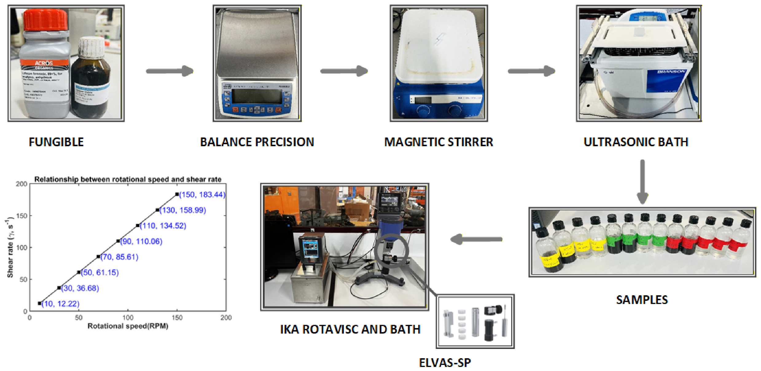
The experimental framework, including the nanofluid preparation protocol, instrumentation, and the calibrated relationship between rotational speed and shear rate, is detailed in Figure 1. For each sample, viscosity and shear stress were measured in triplicate across a shear rate range of 10–150 RPM and temperatures from 25–60 °C. All reported data are mean values with uncertainties, Equation (1), given at the 95% confidence level. Total uncertainty was computed as the quadratic sum of instrumental accuracy and statistical uncertainty:

$${\sigma }_{\mathrm{visc}}=\sqrt{{\sigma }_{\mathrm{accuracy}}^2+{\left(t_{95}{\displaystyle \frac{s_{\mathrm{visc}}}{\sqrt{m}}}\right)}^2}$$

(1)

where ${\sigma }_{\mathrm{accuracy}}$ is the actual measurement accuracy for each test condition, which depends on the rotational speed (RPM) employed and is provided by the instrument. $s_{\mathrm{visc}}$ is the sample standard deviation, m the number of measurements, and $t_{95}$ the Student’s t factor for 95% confidence.

The system was ensured to remain stable during all measurements. Prior to each experiment, samples were equilibrated in a temperature-controlled bath to guarantee thermal stability. During measurements, continuous rotation was maintained, and the total measurement time was kept shorter than the timescale over which any static changes in the sample could be visually observed. No sedimentation or particle agglomeration was detected, and therefore, no dispersing agents were required, as the suspension remained stable throughout the measurement period. Additionally, the exposed surface area was sufficiently small to render evaporation and absorption effects negligible.

Visual inspection to verify stability of the nanofluid has been reported previously in the literature in much research, alone or in combination with other techniques. For example, the following works include only visual inspection to check stability: Momin et al. (2025) [65] for the H₂O-based MgO, ZnO, and MWCNT nanofluid, Jia et al. (2025) [66] for lubricating oil including CuO nanoparticles, Muzhanje et al. (2025) [67] using CuO/Al₂O₃ nanoparticles mixed with PCMs, Sofiah et al. (2023) [68] employing CuO/Polyaniline nanocomposites-blended in palm oil, and Sofiah et al. (2022) [69] using CuO in palm olein. A quantitative indicator that confirms that concentration is retained after heating is that no significant change in the viscosity measurements for each experimental point occurs. Each measurement was repeated at least 3 times, and the relative standard deviations were very low (average value of 2.2%). In addition to this, no experimental evidence of viscosity trend (for example, viscosity increase due to concentration change) was observed.

The viscosity characterization behavior was performed using linear regression analysis to evaluate flow consistency and the constitutive behavior of the fluids. By applying the Power Law model (Ostwald–de Waele), as in Abbas 2022 [28], $\tau =k{\gamma }^n$, the flow behavior index (n) was quantified by linearizing the relationship as follows:

$${log}_{10}\left(\tau \right)=n{log}_{10}\left(\gamma \right)+{log}_{10}\left(k\right)$$

(2)

where $\tau$ represents the shear stress, $\gamma$ denotes the shear rate, and k is the consistency index.

Following Newton’s law of viscosity, the dynamic viscosity $\mu$ is defined as the ratio between shear stress and shear rate:

$$\mu ={\displaystyle \frac{\tau }{\gamma }}$$

(3)

2.2. Machine Learning Regression Techniques

The experimental data collected to characterize viscosity were used to develop a predictive model estimating viscosity as a function of H₂O–LiBr and CuO concentrations, shear rate, and temperature. The system exhibits well-defined and experimentally consistent trends, where viscosity increases with H₂O–LiBr concentration, decreases with CuO content and temperature, and shows a non-monotonic dependence on shear rate. These coupled nonlinear interactions motivate the use of data-driven regression approaches, since deriving an explicit constitutive equation from first principles is non-trivial within the explored experimental domain.

To capture the combined effect of these concurrent trends, a comparative modeling strategy was adopted to evaluate both linear and nonlinear functional approximations of increasing flexibility. Polynomial regression (PR) and ridge regression (RR) were used as interpretable parametric baselines, while random forest (RF), support vector regression (SVR), k-nearest neighbors (KNN), and multi-layer perceptron (MLP) were employed as non-parametric and machine-learning-based approaches capable of learning more flexible input–output mappings. This framework enables a systematic assessment of model performance under different functional assumptions without imposing a predefined constitutive equation. Instead, the models learn the underlying mapping directly from data, allowing flexible approximation of potentially nonlinear and coupled dependencies within the investigated parameter space.

Before applying any regression or machine learning model, feature scaling was performed to prevent variables with larger magnitudes from dominating the learning process. Each feature was standardized to have a zero mean and unit variance, according to

$$x^{\prime }={\displaystyle \frac{x-\overline{x}}{{\sigma }_x}}$$

(4)

A total of 558 samples were obtained and randomly partitioned into 372 training samples (≈67%) and 186 independent test samples (≈33%). The test set was kept strictly independent and was not used during model training or hyperparameter optimization, ensuring an unbiased evaluation of generalization performance.

Hyperparameter optimization was performed using repeated 5-fold cross-validation with three repetitions. This strategy reduces variance associated with data partitioning and provides a more robust estimate of generalization performance, particularly for moderately sized datasets.

Linear models (PR and RR) were evaluated across multiple polynomial degrees to capture nonlinear relationships explicitly. In contrast, nonlinear models (RF, SVR, KNN, and MLP) were trained on the original feature space, as their internal structures inherently allow flexible nonlinear function approximation. The full search space for all models is summarized in

Table 2. Hyperparameter search spaces and optimization strategy for all regression models.

Model	Hyperparameter Space	Search Size
PR	Degree $\{1,2,3\}$ Intercept: True, False	6
RR	Degree $\{1,2,3\}$ $\alpha \in [{10}^{-4},{10}^{-2}]$ (100 log-spaced)	300
RF	$n_{estimators}\{50,100,150,200\}$ Depth $\{3,5,7,\infty \}$ Leaf $\{1,2,3\}$	48
SVR	Kernel: rbf, poly $C\in [{10}^{-2},{10}^2]$ $\gamma \in \{0.001,0.01,0.1,1,scale,auto\}$ $ϵ\in \{0.001,0.01,0.1,0.5\}$	960
KNN	$k\{2,3,5,7,10,15\}$ Weights: uniform, distance $p\{1,2,3\}$ Metric: minkowski, chebyshev, manhattan, euclidean Algorithm: auto, ball_tree, kd_tree, brute	576
MLP	Architecture: 1–2 layers, 2–18 neurons (sampled) $\alpha \in \{{10}^{-4},{10}^{-3.33},{10}^{-2.66},{10}^{-2}\}$ Solver: lbfgs, adam	720

.

Multiple metrics were used to evaluate model performance, providing a comprehensive assessment of predictive accuracy. The coefficient of determination ($R^2$) was used as the primary optimization criterion and as the refit score for model selection in the grid search procedure (

Table 3. Evaluation metrics employed for regression model assessment.

Metric	Formula
Mean Absolute Error (MAE)	${\displaystyle MAE=\mathrm{Median}\left(\right|y_i-{\widehat{y}}_i\left|\right)}$
Root Mean Squared Error (RMSE)	${\displaystyle RMSE=\sqrt{\frac{1}{n_s}\sum _{i=1}^n{(y_i-{\widehat{y}}_i)}^2}}$
Coefficient of Determination ($R^2$)	${\displaystyle R^2=1-\frac{{\sum }_{i=1}^{n_s}{(y_i-{\widehat{y}}_i)}^2}{{\sum }_{i=1}^{n_s}{(y_i-\overline{y})}^2}}$
Mean Absolute Percentage Error (MAPE)	${\displaystyle MAPE=\frac{100}{n_s}{\displaystyle \sum _{i=1}^{n_s}}\left|\frac{y_i-{\widehat{y}}_i}{y_i}\right|}$
Maximum Absolute Error (MAXE)	${\displaystyle MAXE=\underset{i}{max}\left|y_i-{\widehat{y}}_i\right|}$

). MAE and RMSE were included to quantify absolute and quadratic errors, respectively. MAPE and MAXE were also computed to assess relative and worst-case deviations.

To ensure reproducibility, all models were implemented using scikit-learn pipelines, guaranteeing that preprocessing and model fitting were performed consistently within each cross-validation fold. This prevents data leakage and ensures that performance metrics reflect true out-of-sample predictive capability.

3. Results and Discussion

3.1. Experimental Results

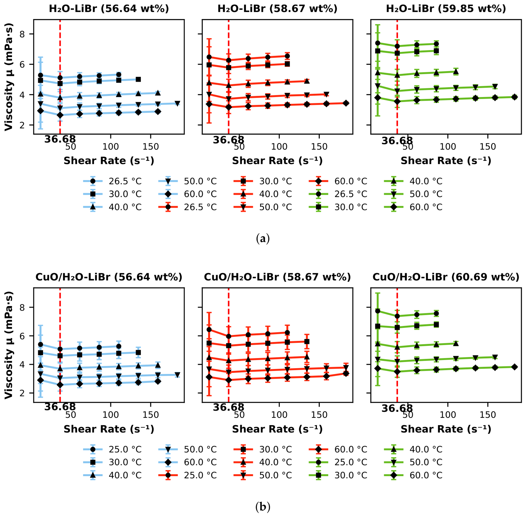
Figure 2 depicts how the viscosity of H₂O–LiBr and CuO/H₂O–LiBr changes with shear rate and temperature for each salt concentration, including measurement uncertainties indicated by error bars. Values shown are the mean of the three measures taken in each experimental condition. A minimum value for the viscosity can be observed at 30 RPM, corresponding to a shear rate of $\gamma =36.68{\mathrm{s}}^{-1}$, followed by a slight increase in viscosity, reaching, at the maximum shear rate tested, a viscosity value similar to the one obtained at 10 RPM ($\gamma =12.22{\mathrm{s}}^{-1}$). The maximum increase was observed for H₂O–LiBr at 50 °C and 150 RPM, reaching 9.95% at 56.64 wt%, and for CuO/H₂O–LiBr at 60 °C and 150 RPM, reaching 16% at 58.67 wt%. As expected, increasing the salt concentration leads to higher viscosity in both the base fluid and the nanofluid, while higher temperatures result in lower viscosity. Approximately, viscosity increases 0.0027 mPa·s/wt% and decreases 0.001 mPa·s/°C. The minimum obtained at 30 RPM can be attributed to the low accuracy of the measurements at 10 RPM, as shown by the error bars in the figure.

The experimental viscosity data for the H₂O–LiBr solution were validated against established predictive models. Specifically, present results were compared with the widely adopted correlation of Lee et al. (1990) [45], as implemented in the Engineering Equation Solver (EES™) [70], and the more recent correlation proposed by Fleßner and Ziegler (2023) [71]. The average absolute relative deviation (AARD) (Equation (5)) was calculated for all experimental points in each model, allowing a comprehensive assessment of predictive performance. For reporting and discussion purposes, the measurements at 30 RPM were taken as a reference case, as they exhibit the lowest deviation with respect to the most recent correlation available in the literature, namely, the model proposed by Fleßner and Ziegler (2023) [71]. The results demonstrate excellent agreement between the present experimental datasets and the theoretical predictions, yielding an AARD of 3.23% for EES™ and 3.59% for the Fleßner and Ziegler model.

$$AARD(\%)={\displaystyle \frac{100}{n}}{\displaystyle \sum _0^n}{\displaystyle \frac{[{\mu }_{cal}-{\mu }_{exp}]}{{\mu }_{exp}}}$$

(5)

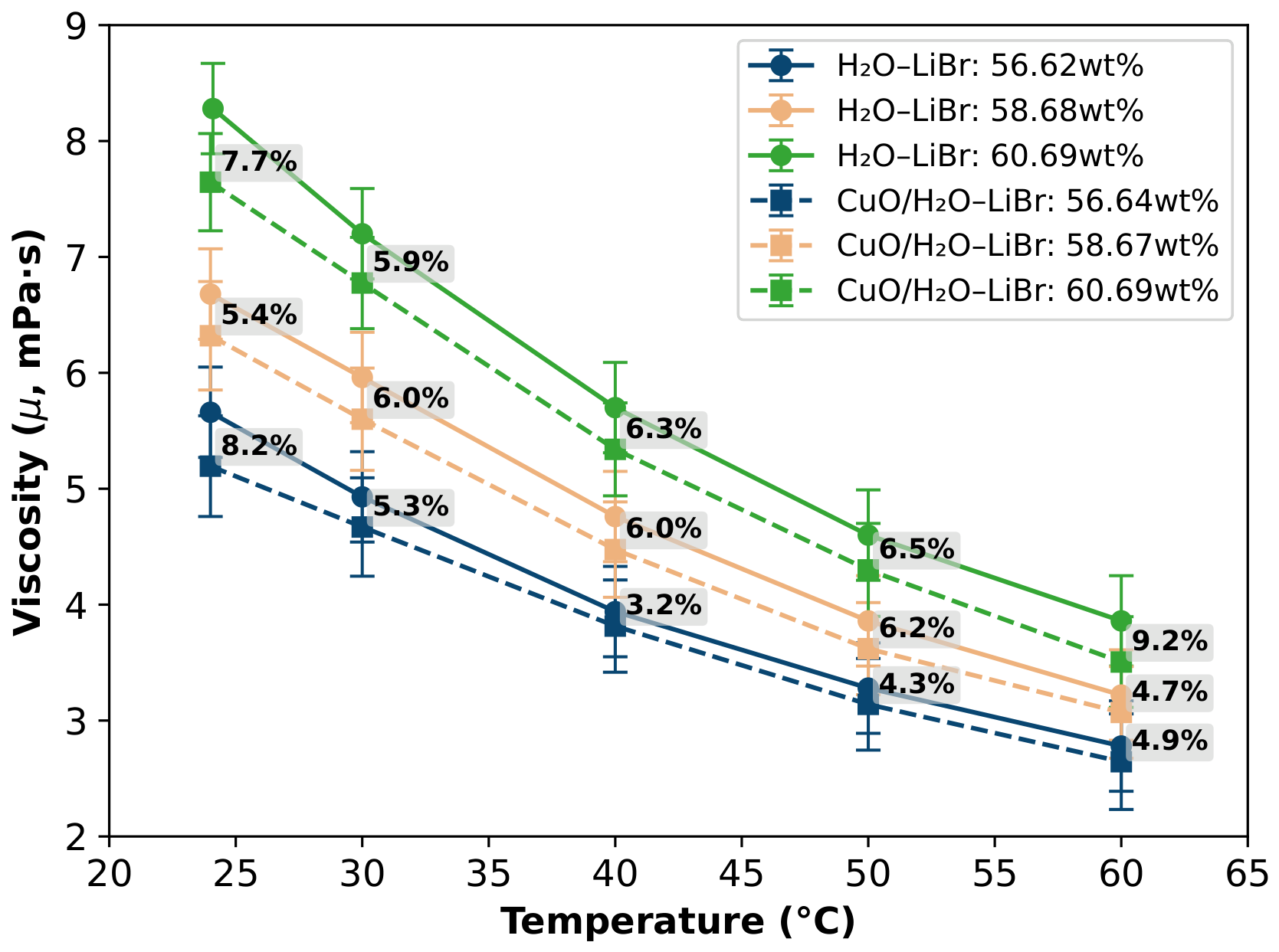
To assess the degree of viscosity reduction (DVR) of the CuO/H₂O–LiBr nanofluid compared to the H₂O–LiBr base fluid, additional viscosity measurements of the base fluid and the nanofluid were conducted at a fixed shear rate of $\gamma =36.68$ ${\mathrm{s}}^{-1}$ (30 RPM). In this case, the large difference in concentration shown in Figure 2 for the most LiBr concentrated solution was avoided using the same concentration (60.69 wt%) in both fluids. This approach was adopted to ensure a meaningful comparison between the base fluid and the nanofluid and to enable a reliable determination of the DVR. The DVR is depicted in Figure 3, showing a significant viscosity reduction ranging from 3.2% to 9.2%, with an average degree of viscosity reduction (ADVR), as per Equation (6), of 5.98%.

$$ADVR(\%)={\displaystyle \frac{100}{n}}{\displaystyle \sum _0^n}{\displaystyle \frac{[{\mu }_{base}-{\mu }_{nanofluids}]}{{\mu }_{base}}}$$

(6)

The measurement accuracy associated with experiments in Figure 3 was 0.39 mPa.s. This accuracy is included in the error bars presented in the figure. As can be observed, even when the experimental results are shifted within the limits defined by the error bars, the same overall trend is maintained. Consequently, the observed viscosity reduction of 3.2–9.2% remains distinguishable from the experimental uncertainty and supports the validity of the reported ADVR values.

Viscosity reduction can be attributed to the possible placement of nanoparticles between the base fluid layers, facilitating the movement of the fluid layers relative to each other and generating a self-lubricating effect. Consequently, the internal resistance to flow decreases, enabling energy transfer via advection and reducing the dynamic viscosity of the nanofluid. In addition, the presence of nanoparticles may disturb the smooth gliding of the fluid layers, introducing micro-scale disruptions that modify the local flow structure and further contribute to the observed changes in viscosity.

It should be highlighted that the present results represent the first study available in the open literature showing the effect of shear rate on the viscosity of the H₂O–LiBr solution. Furthermore, for the first time, the viscosity of the CuO-based nanofluid is evaluated at 0.1 wt% concentration. Viscosity is a very important thermophysical property that notably influences heat, momentum, and mass transfer processes in absorption systems, as demonstrated by Mittermaier and Ziegler (2018) [72], Yang et al. (2011a) [39] and Yang et al. (2011b) [38]. Previous data available for viscosity of the H₂O–LiBr solution, used by Fleßner and Ziegler (2023) [71] to develop a new correlation, only include data as a function of temperature and concentration. Novel results presented in this research allow a more precise viscosity prediction for the H₂O–LiBr solution and its CuO-based nanofluid.

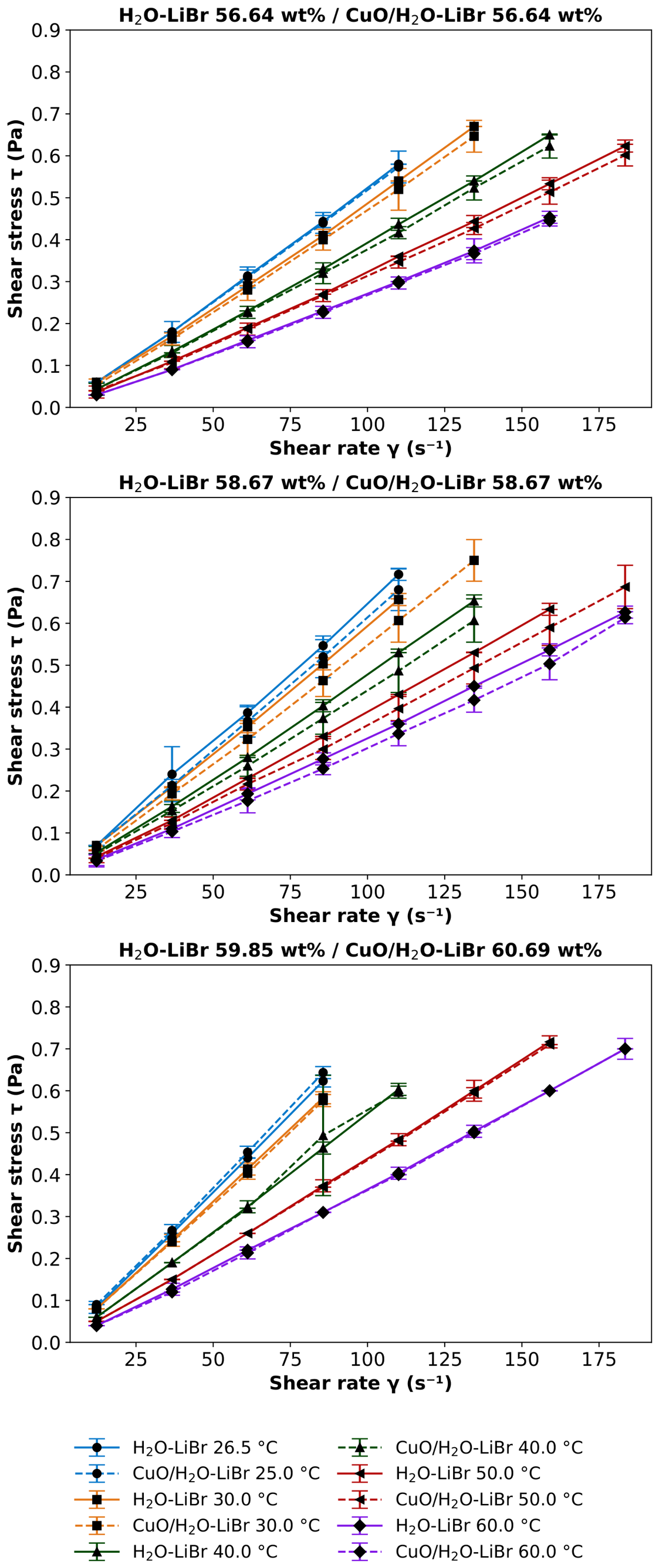
Figure 4 presents the shear stress vs. shear rate, including the corresponding error bars for each measurement, and these data are the ones used to evaluate dilatancy of the base fluid and the nanofluid. The figure compares the base fluid H₂O–LiBr and the nanofluid CuO/H₂O–LiBr, and the same increasing trend is observed. Additionally, for the nanofluid, a reduction of the shear stress compared to the base fluid can be observed. This reduction made it possible to apply higher shear rates, which the base fluid.

The results presented in Figure 2 and Figure 4 correspond to the same set of samples. In contrast, the results shown in Figure 3 were obtained from different samples tested under different operating conditions. Consequently, different concentrations and temperatures appear in the figures because they correspond to the specific samples that were experimentally analyzed under each set of conditions.

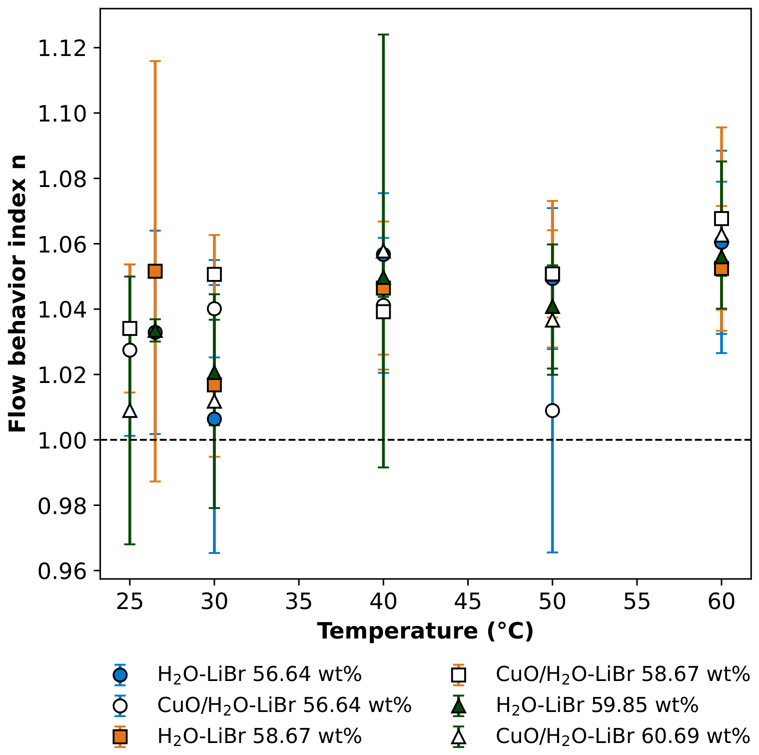
The flow behavior index n (Equation (1)) was determined via polynomial fitting for both H₂O–LiBr and CuO/H₂O–LiBr systems, Figure 5. For all temperatures and compositions evaluated, the calculated values satisfy $n>1$, indicating a slight shear-thickening (dilatant) behavior. This trend is consistent with the rheological response presented in Figure 2, where viscosity shows a modest increase with increasing shear rate. The uncertainty associated with n was estimated from the standard error of the regression slope using a 95% confidence interval and is represented by the error bars in Figure 5. Despite the relatively small deviations observed among conditions, the regressions exhibited excellent agreement with the experimental data, with coefficients of determination exceeding $R^2>0.996$ across all experimental conditions.

3.2. Regression Model Using Machine Learning Techniques

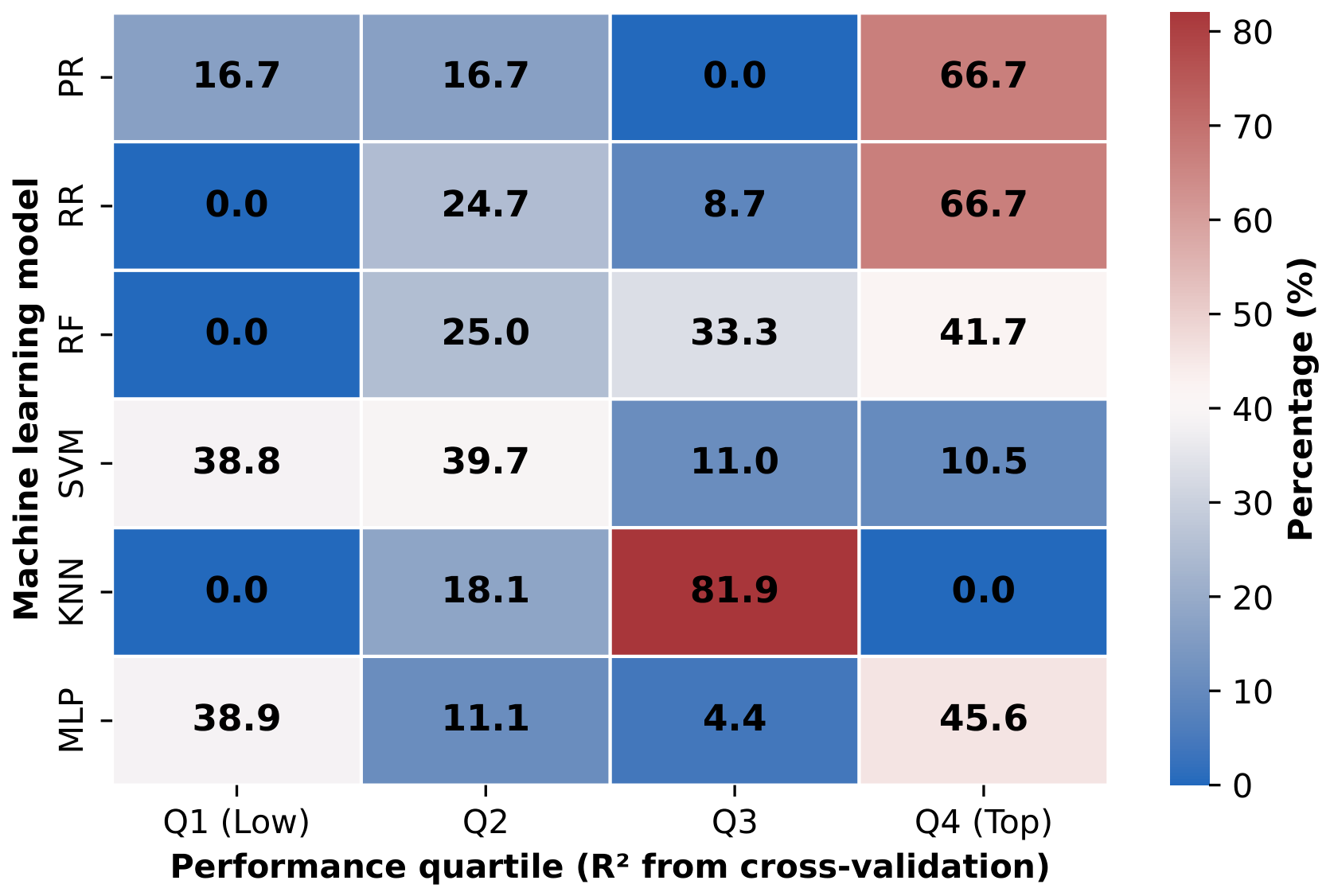
The distribution of model performance across $R^2$ quartiles (Figure 6) reveals distinct sensitivity profiles for each architecture. SVR exhibited the highest susceptibility to hyperparameter configurations, with nearly half of its trials, 48%, relegated to the lowest performance quartile ($Q_1$). In stark contrast, KNN demonstrated exceptional stability, with 81.9% of its instances falling within the third quartile ($Q_3$), yet it consistently failed to reach the top-tier performance threshold. Across the entire experimental space, only 25% of the 2610 configurations reached the fourth quartile ($Q_4$). The most robust predictive capabilities were consistently observed in the MLP and RR models, which successfully populated the elite $Q_4$ bracket with 45.6% and 66.7% configurations, respectively.

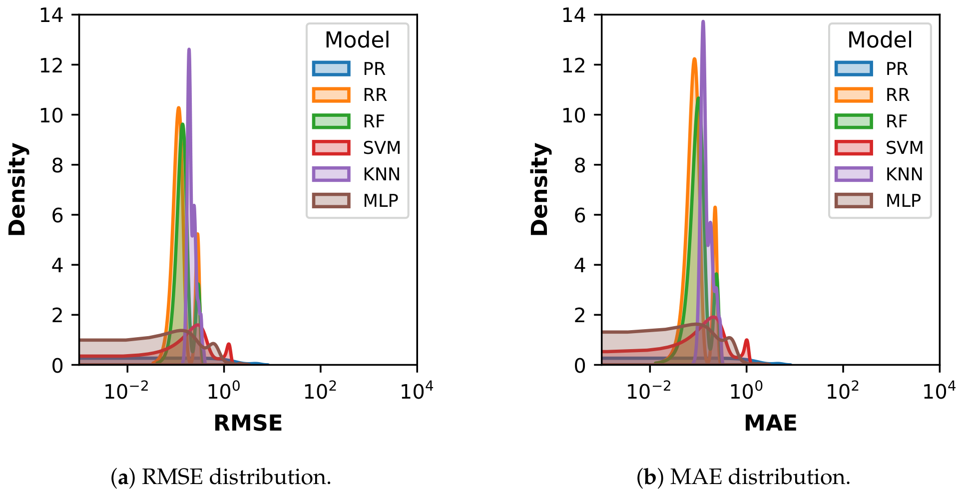
The comparative analysis of the error distributions shown in Figure 7 provides valuable insights into model stability. Although connectionist models such as the MLP achieved the highest predictive performance, their broader error distributions reveal a pronounced sensitivity to architectural design and initialization parameters. In contrast, RR and KNN models exhibited narrower, more leptokurtic distributions, suggesting more consistent generalization across the experimental range.

Table 4. Top 10 models’ performance based on cross-validation metrics.

Rank	Model	Key Parameters	${\mathit{R}}^2$ (CV)	RMSE (CV)	MAE (CV)
1	MLP	{act: ’tanh’, $\alpha$: 0.01, hls: (4, 2)}	$0.9923\pm 0.0025$	$0.1084\pm 0.0201$	$0.0754\pm 0.0107$
2	MLP	{act: ’tanh’, $\alpha$: 0.01, hls: (4, 6)}	$0.9922\pm 0.0030$	$0.1085\pm 0.0221$	$0.0722\pm 0.0084$
3	MLP	{act: ’tanh’, $\alpha$: $4.64\times {10}^{-4}$, hls: (4, 2)}	$0.9922\pm 0.0028$	$0.1086\pm 0.0210$	$0.0760\pm 0.0090$
4	MLP	{act: ’tanh’, $\alpha$: 0.01, hls: (4,)}	$0.9922\pm 0.0040$	$0.1074\pm 0.0281$	$0.0711\pm 0.0104$
5	MLP	{act: ’tanh’, $\alpha$: 0.0001, hls: (6,)}	$0.9921\pm 0.0030$	$0.1091\pm 0.0211$	$0.0741\pm 0.0090$
6	MLP	{act: ’tanh’, $\alpha$: 0.0001, hls: (4, 2)}	$0.9921\pm 0.0028$	$0.1095\pm 0.0209$	$0.0768\pm 0.0090$
7	MLP	{act: ’tanh’, $\alpha$: 0.01, hls: (6,)}	$0.9920\pm 0.0030$	$0.1098\pm 0.0223$	$0.0762\pm 0.0118$
8	MLP	{act: ’tanh’, $\alpha$: $4.64\times {10}^{-4}$, hls: (6,)}	$0.9920\pm 0.0033$	$0.1092\pm 0.0231$	$0.0742\pm 0.0122$
9	RR	{$\alpha$: 0.01, poly_deg: 3}	$0.9920\pm 0.0028$	$0.1101\pm 0.0210$	$0.0783\pm 0.0094$
10	RR	{$\alpha$: 0.0095, poly_deg: 3}	$0.9920\pm 0.0028$	$0.1101\pm 0.0210$	$0.0783\pm 0.0094$

summarizes the performance metrics of the ten best model configurations identified through exhaustive hyperparameter optimization. The results are ranked according to the mean cross-validation (CV) $R^2$, along with the corresponding RMSE and MAE. The use of repeated 5-fold cross-validation, which facilitates the evaluation of multiple configurations to identify the optimal model based on statistical stability rather than manual selection.

The MLP dominates this task, occupying 80% of the top ten positions. The best configuration (Rank 1) achieved a near-perfect fit ($R^2=0.9923$) with a shallow 4–2 architecture and a (tanh) activation function, indicating that optimal performance can be achieved efficiently with a minimal risk of overfitting.

RR with a third-degree polynomial expansion remains competitive (ranks 9–10), indicating that the underlying nonlinear relationship still exhibits a pronounced polynomial character. The strong presence of RR in Q4, as shown in Figure 6, suggests that the dependence of viscosity on concentration and temperature, despite being nonlinear, retains a structure that can be efficiently represented by regularized polynomial models.

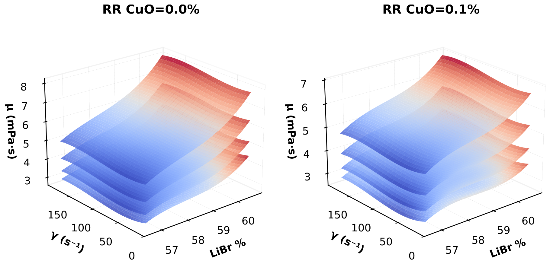
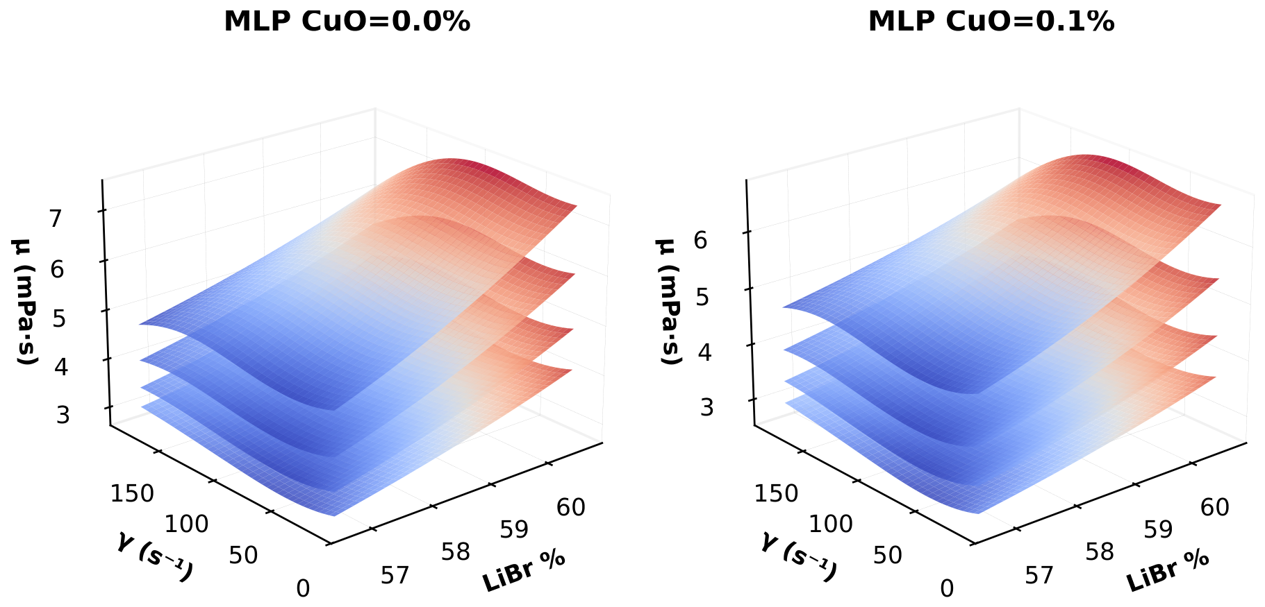
However, while linear and polynomial regressions are restricted to predefined functional forms that impose rigid trends (Figure 8), the MLP’s layered structure allows the non-linear curvature of viscosity relative to shear rate, (Figure 9).

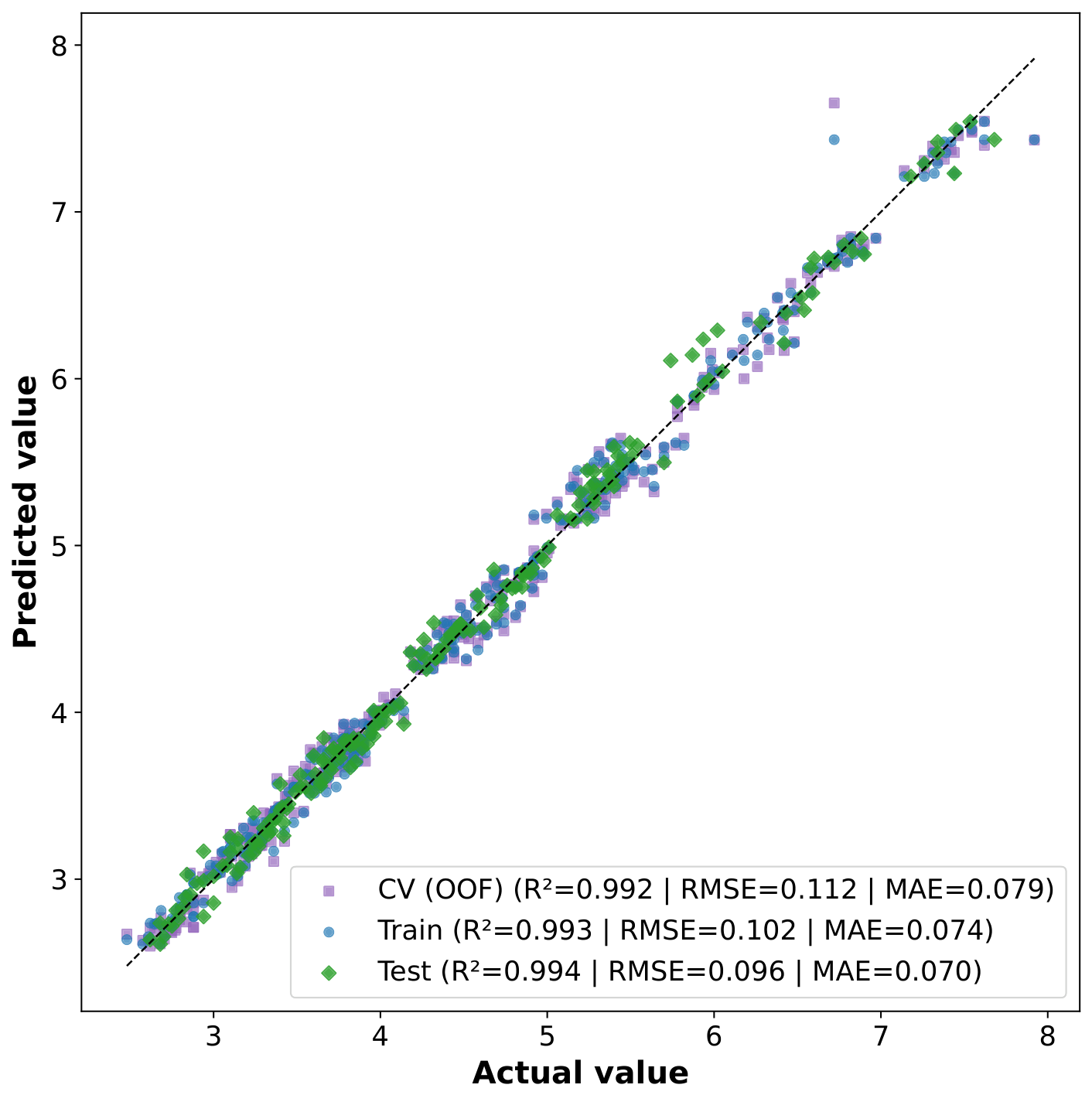
In the following analysis, all results correspond to the best-performing model (Rank 1). Figure 10 presents the predicted vs. actual values for the training, cross-validation, and test sets, confirming the excellent generalization capability of the model. The actual values used in the procedure correspond to the experimental values for each measurement; their 2% accuracy is not shown in the figure to maintain clarity and improve data reading.

Furthermore, the low and consistent MAPE values (1.71% for training and 1.63% for testing) and MAXE values (10.6% for training and 7.7% for testing) support the absence of overfitting.

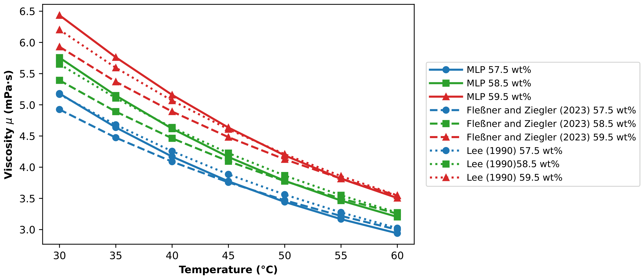
The main advantages of the proposed model lie in its ability to accurately predict both the viscosity of the base fluid and the nanofluid and the inclusion of the shear rate in the model. In addition to this, up to now, there are no previous theoretical models able to predict the viscosity of the nanofluid. With respect to the base fluid, there are some models, and they can still be used, but without the influence of the shear rate. The largest deviation from the experiment of these models was obtained with Fleßner and Ziegler (2023) [71], yielding an AARD of 6.03% at 10 RPM and 4.85% at 150 RPM. For Lee et al. (1990) [45], the AARD was 3.57% at 10 RPM and 3.80% at 150 RPM. A direct comparison between predictions of correlations [71] and [45] and the current MLP model appears in Figure 11, showing an excellent agreement, mainly with [45].

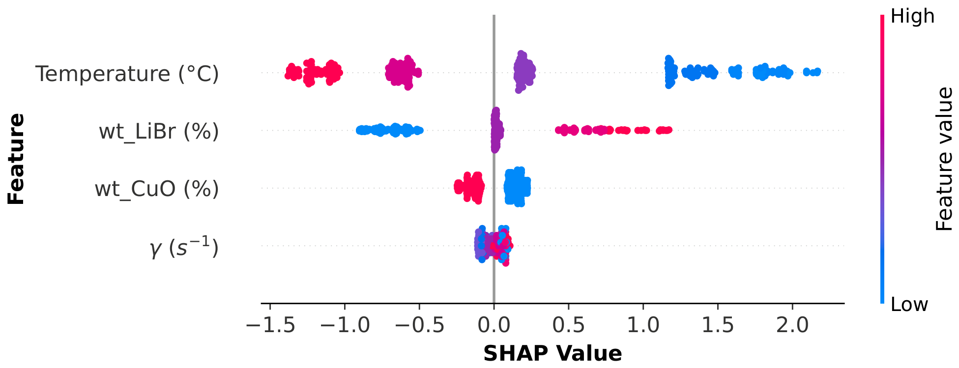
To enhance model transparency and verify its consistency with physical principles, a SHAP (SHapley Additive exPlanations) summary plot was employed (Figure 12). This game-theory-based method quantifies both the magnitude and direction of each feature’s contribution to the predicted viscosity.

The SHAP analysis reveals that temperature is the dominant factor governing viscosity, followed by LiBr concentration ($wt\text{\_}LiBr$). Higher temperatures (red markers) are associated with negative SHAP values, confirming the expected physical trend of viscosity reduction with increasing temperature. Conversely, higher LiBr concentrations shift SHAP values positively, indicating a direct increase in predicted viscosity. The nanoparticle concentration ($wt\text{\_}CuO$) shows a more moderate effect, contributing with a lower overall impact than the base fluid components. Finally, the shear rate ($\gamma$) shows a narrow SHAP distribution, indicating a subtle influence compared to dominant thermal effects. This aligns with the experimental flow behavior index (n), which remains close to unity with a slight shear-thickening tendency ($n>1$). While the MLP architecture is structurally capable of capturing these non-Newtonian nuances, the analysis confirms that shear rate acts as a secondary fine-tuning factor within this specific experimental range.

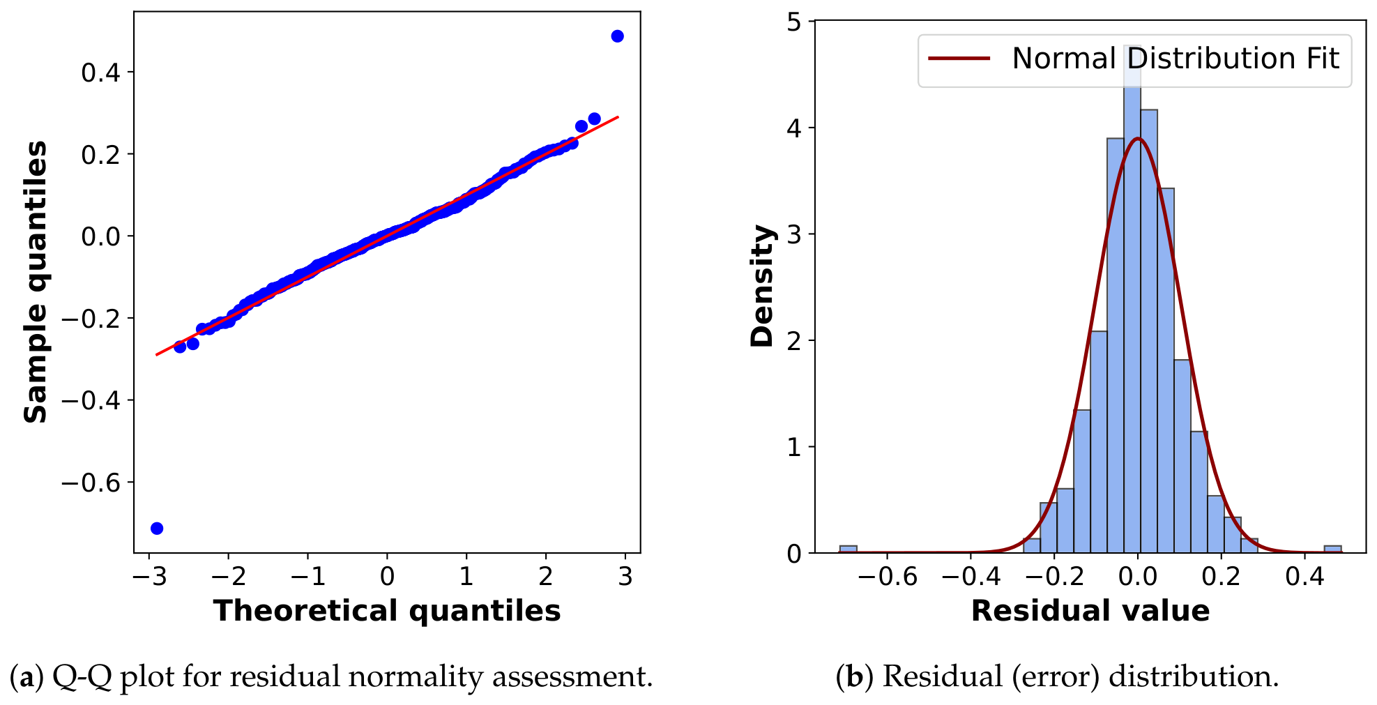
Figure 13 presents the Q-Q plot and histogram for residual analysis. The Q-Q plot confirms that most points closely follow the diagonal, with minor deviations at the tails typical of experimental data, which do not compromise the model’s validity. The histogram indicates that prediction errors are centered around zero and approximately normally distributed, suggesting random errors without systematic bias.

3.3. Design and Implementation of MLP-Based Prediction Graphical User Interface (GUI)

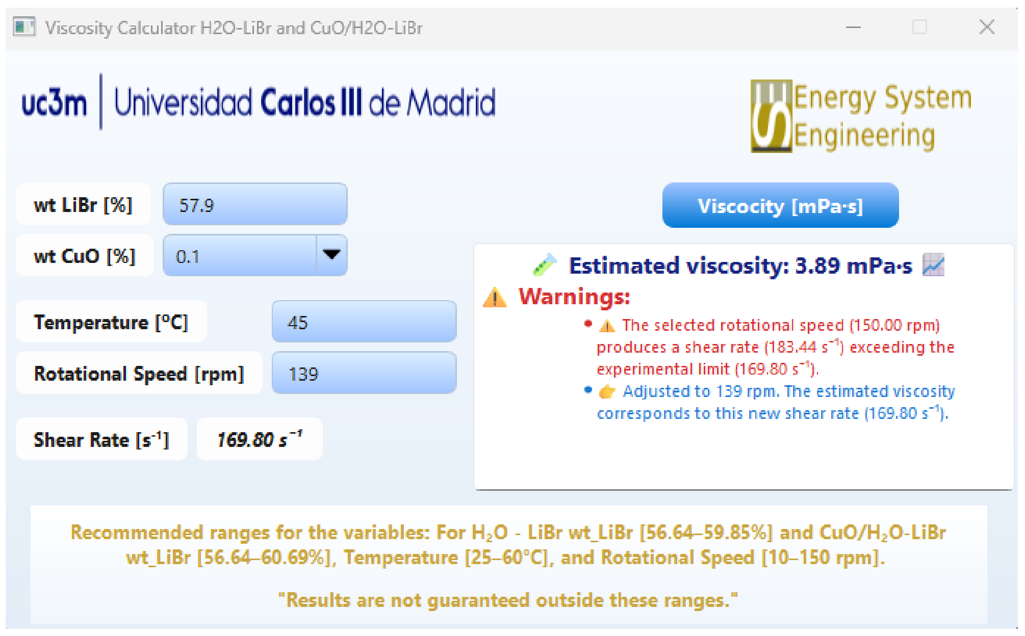
As determined in the previous section, the best model for predicting the experimental data was the MLP, which was therefore used to develop a graphical application in Python 3.13.7 using the PySide6 library and Qt Designer. The program was exported as a standalone executable (.exe), which does not require Python for its execution, Figure 14. The application allows the estimation of the viscosity of H₂O–LiBr and CuO/H₂O–LiBr solutions based on the LiBr concentration [56.64–60.69 wt%], CuO content [0 and 0.1 wt%], temperature [25–60 °C], and shear rate. The shear rate is expressed as a linear function of the rotation speed [10–150 RPM]. The prediction tool is available on the web page of the research group (https://ise.uc3m.es/projects/pvabs-2/ (accessed 6 July 2026)).

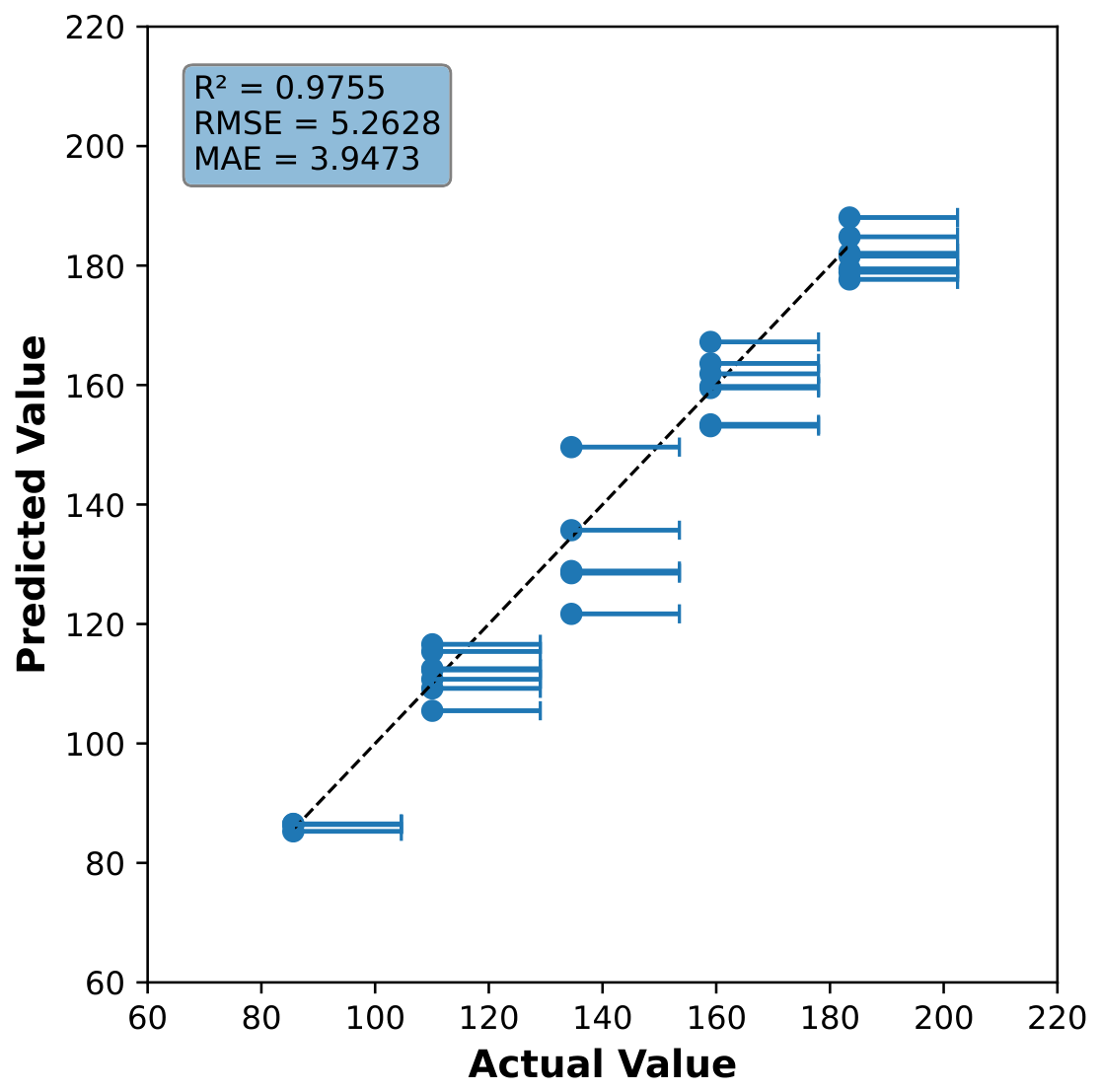
As observed in the results presented in the previous sections, due to the shear-thickening behavior of the fluid at different LiBr and CuO concentrations and temperatures, there exists a maximum shear rate at which the sample can be tested. The measurements were conducted in increments of 20 RPM, so the true maximum shear rate could potentially occur 19 RPM beyond the maximum measured value, as illustrated in Figure 15. To predict this maximum shear rate, a linear regression adjustment using a cubic model was performed, yielding a coefficient of determination $R^2=0.975$, (Figure 15).

The GUI is designed to be intuitive and user-friendly, incorporating several warning messages to inform users when the selected operating conditions fall outside the validated experimental ranges. To estimate the viscosity, the user must enter the LiBr concentration (wt%), specify the CuO concentration (wt%), as well as the temperature (°C) and the rotational speed (RPM). The rotational speed is automatically converted into the corresponding shear rate (${\mathrm{s}}^{-1}$). If the calculated shear rate exceeds the maximum experimental limit of the available dataset, the software automatically adjusts it to the highest valid value. A warning message is displayed to notify the user of this correction, and the predicted viscosity is then calculated and reported for the adjusted shear rate. This ensures that all viscosity predictions remain within the range supported by the experimental data.

Nevertheless, an explicit engineering correlation may be useful for practical applications. For this reason, the mathematical expression corresponding to the RR model, Equation (7), corresponding to Rank 9 in the Table 4, has been included.

$$\mu =4.16363+{\displaystyle \sum _{j=1}^{34}}{k}_j·w{t}_{LiBr}^{a_j}·T^{b_j}·w{t}_{CuO}^{c_j}·{\gamma }^{d_j}$$

(7)

Coefficients and exponents appear in

Table 5. Coefficients and exponents for Equation (7).

j	${\mathit{a}}_{\mathit{j}}$	${\mathit{b}}_{\mathit{j}}$	${\mathit{c}}_{\mathit{j}}$	${\mathit{d}}_{\mathit{j}}$	${\mathit{k}}_{\mathit{j}}$
1	1	0	0	0	$1.57559\times {10}^{-1}$
2	0	1	0	0	$-5.52354\times {10}^{-1}$
3	0	0	1	0	$-6.44203\times {10}^{-2}$
4	0	0	0	1	$6.41021\times {10}^{-2}$
5	2	0	0	0	$5.29566\times {10}^{-2}$
6	1	1	0	0	$-1.92043\times {10}^{-1}$
7	1	0	1	0	$-1.32302\times {10}^{-1}$
8	1	0	0	1	$1.60228\times {10}^{-2}$
9	0	2	0	0	$2.23142\times {10}^{-1}$
10	0	1	1	0	$3.02445\times {10}^{-2}$
11	0	1	0	1	$-2.24414\times {10}^{-2}$
12	0	0	2	0	$1.38546\times {10}^{-3}$
13	0	0	1	1	$-2.98300\times {10}^{-3}$
14	0	0	0	2	$8.60428\times {10}^{-2}$
15	3	0	0	0	$1.87956\times {10}^{-1}$
16	2	1	0	0	$-2.58163\times {10}^{-2}$
17	2	0	1	0	$-6.97083\times {10}^{-2}$
18	2	0	0	1	$2.91850\times {10}^{-3}$
19	1	2	0	0	$3.31429\times {10}^{-2}$
20	1	1	1	0	$2.50141\times {10}^{-2}$
21	1	1	0	1	$-6.25007\times {10}^{-3}$
22	1	0	2	0	$1.60404\times {10}^1$
23	1	0	1	1	$6.34838\times {10}^{-3}$
24	1	0	0	2	$-7.33885\times {10}^{-3}$
25	0	3	0	0	$-5.31111\times {10}^{-3}$
26	0	2	1	0	$-5.10739\times {10}^{-3}$
27	0	2	0	1	$2.16953\times {10}^{-3}$
28	0	1	2	0	$-5.53004\times {10}^{-1}$
29	0	1	1	1	$6.30461\times {10}^{-3}$
30	0	1	0	2	$1.75992\times {10}^{-2}$
31	0	0	3	0	$-6.44501\times {10}^{-2}$
32	0	0	2	1	$6.41662\times {10}^{-2}$
33	0	0	1	2	$3.74642\times {10}^{-3}$
34	0	0	0	3	$-5.29883\times {10}^{-2}$

. As explained in Section 2.2 (see Equation (4)), all variables were scaled so that their values ranged between 0 and 1. For this reason, to use Equation (4), the input values should be scaled accordingly. The parameters used for the scaling appear in

Table 6. Parameters for Equation (4).

Variable x	$\overline{\mathit{x}}$	${\mathit{\sigma }}_{\mathit{x}}$
$w{t}_{LiBr}$	58.43313	1.49345
T	43.54032	12.57936
$w{t}_{CuO}$	$5.05376\times {10}^{-2}$	$4.99997\times {10}^{-2}$
$\gamma$	79.55473	49.07259

.

4. Conclusions

In this research, novel experimental results are presented for the viscosity of the H₂O–LiBr solution and the CuO/H₂O–LiBr nanofluid. For the first time, the effect of shear rate on the viscosity of this solution and its CuO-based nanofluid has been evaluated, and additionally, new data for the pure CuO/H₂O–LiBr nanofluid have been obtained. Temperatures have been modified between 24 and 60 °C, mass fractions of salt in the base fluid from 56.62 to 60.69 wt%, while the nanoparticle concentration was fixed at 0.1 wt%. These novel results allow a more precise viscosity prediction for the H₂O–LiBr solution and its CuO-based nanofluid. From this research, the following conclusions have also been reached:

• The viscosity data analysis indicates that the H₂O–LiBr solution and its CuO-based nanofluid exhibit dilatant behavior, with viscosity increasing slightly as the shear rate rises. Within the tested shear rate range (10 to 150 RPM), the maximum viscosity increase observed for CuO/H₂O–LiBr was 16% at 60 °C, 150 RPM, and a concentration of 58.67 wt%. The minimum viscosity in all of the cases corresponded to a shear rate of 36.68 ${\mathrm{s}}^{-1}$ (30 RPM). Viscosity values obtained under this condition for the H₂O–LiBr solution agree very well with those obtained using the correlation of Lee et al. (1990) [45] (average absolute relative deviation equal to 3.23%) and using that of Fleßner and Ziegler (2023) [71] (3.59%).
• A comparison between the nanofluid and the base fluid reveals a notable reduction in the viscosity of the nanofluid, with an average degree of viscosity reduction of 5.98%. These results indicate potential improvements in mass and heat transfer processes within the absorption machine, accompanied by reduced pressure drops and lower pump energy consumption.
• An AI-based predictive framework has been developed to determine the viscosities of the nanofluid and base fluid, demonstrating excellent agreement with experimental data. Furthermore, a standalone executable (.exe) with an intuitive GUI has been provided, enabling users to obtain accurate predictions without local Python installation. The Python-based source code is available upon request.

The main limitation of this research is the use of only one concentration of nanoparticles. Future research could include the use of other nanoparticle concentrations, covering a range close to the optimum value (0.1 wt%) found in reference [2] for mass transfer. In this way, the concentration corresponding to the minimum viscosity can be confirmed or identified. In this experimental study, potential sources of errors include the high uncertainty at low shear rates. The use of viscometers with higher accuracy in this region are recommended for future research.

References

1. Venegas, M.; de Vega, M.; García-Hernando, N. Performance improvement of absorption chillers: A review on nanoparticle addition. Renew. Sustain. Energy Rev. 2025, 208, 115008. [Google Scholar] [CrossRef]
2. Wang, G.; Zeng, M.; Zhang, Q. Experimental investigation of saturated pressure and mass transfer characteristics of nano-lithium bromide solution. Int. Commun. Heat Mass Transf. 2020, 115, 104605. [Google Scholar] [CrossRef]
3. Zeiny, A.; Haruna, M.; Wen, D. Aqueous lithium bromide nanosolution for solar absorption refrigeration systems. AIP Conf. Proc. 2019, 2123, 020083. [Google Scholar] [CrossRef]
4. Yildiz, A.; Sunal, S. The effect of CuO and TiO2 nano particles on energy and exergy performance in diffusion absorption refrigeration system. ISI Bilim Tek. Derg. 2023, 43, 41–58. [Google Scholar] [CrossRef]
5. Bhat, A.Y.; Qayoum, A. Viscosity of CuO nanofluids: Experimental investigation and modelling with FFBP-ANN. Thermochim. Acta 2022, 714, 179267. [Google Scholar] [CrossRef]
6. Einstein, A. Eine neue Bestimmung der Moleküldimensionen. Ann. Phys. 1906, 324, 289–306. [Google Scholar] [CrossRef]
7. Batchelor, G. The effect of Brownian motion on the bulk stress in a suspension of spherical particles. J. Fluid Mech. 1977, 83, 97–117. [Google Scholar] [CrossRef]
8. Nielsen, L.E. Generalized Equation for the Elastic Moduli of Composite Materials. J. Appl. Phys. 1970, 41, 4626–4627. [Google Scholar] [CrossRef]
9. Nguyen, C.; Desgranges, F.; Roy, G.; Galanis, N.; Maré, T.; Boucher, S.; Angue Mintsa, H. Temperature and particle-size dependent viscosity data for water-based nanofluids—Hysteresis phenomenon. Int. J. Heat Fluid Flow 2007, 28, 1492–1506. [Google Scholar] [CrossRef]
10. Chen, H.; Ding, Y.; Tan, C. Rheological behaviour of nanofluids. New J. Phys. 2007, 9, 367. [Google Scholar] [CrossRef]
11. Su, F.; Ma, X.; Lan, Z. The effect of carbon nanotubes on the physical properties of a binary nanofluid. J. Taiwan Inst. Chem. Eng. 2011, 42, 252–257. [Google Scholar] [CrossRef]
12. Chon, C.; Kihm, K.; Lee, S.; Choi, U. Empirical correlation finding the role of temperature and particle size for nanofluid (Al2O3) thermal conductivity enhancement. Appl. Phys. Lett. 2005, 87, 153107. [Google Scholar] [CrossRef]
13. Wang, G.; Dong, P.; Lu, Y.; Zeng, M.; Zhang, Q. Experimental and theoretical investigation on the surface tension of nano-Lithium Bromide solution. Int. Commun. Heat Mass Transf. 2021, 123, 105231. [Google Scholar] [CrossRef]
14. Fahar, M.; Otanicar, T. Experimental and theoretical description of a technique for the concentration measurement of binary liquids containing nanoparticles. Int. J. Heat Mass Transf. 2015, 85, 561–567. [Google Scholar] [CrossRef]
15. Hamilton, R.; Crosser, O. Thermal conductivity of heterogeneous two-component systems. Ind. Eng. Chem. Fundam. 1962, 1, 187–191. [Google Scholar] [CrossRef]
16. Yang, L.; Du, K.; Ding, Y.; Cheng, B.; Li, Y. Viscosity-prediction models of ammonia water nanofluids based on various dispersion types. Powder Technol. 2012, 215, 210–218. [Google Scholar] [CrossRef]
17. Einstein, A. A new determination of molecular dimensions. Ann. Phys.-Berl. 1906, 4, 37–62. [Google Scholar]
18. Li, J.; Wang, G.; Li, J.; Li, X.; Liu, Y.; Zhang, Q. Empirical model for fitting the viscosity of lithium bromide solution with CuO nanoparticles and E414. Front. Energy Res. 2023, 10, 1093424. [Google Scholar] [CrossRef]
19. Jamal-Abad, M.; Dehghan, M.; Saedodin, S.; Valipour, M.; Zamzamian, A. An experimental investigation of rheological characteristics of non-Newtonian nanofluids. J. Heat Mass Transf. Res. 2014, 1, 17–23. [Google Scholar]
20. Basu, R.; Kinnamon, D.; Skaggs, N.; Womack, J. Faster in-plane switching and reduced rotational viscosity characteristics in a graphene-nematic suspension. J. Appl. Phys. 2016, 119, 185107. [Google Scholar] [CrossRef]
21. Elsoudy, S.; Akl, S.; Abdel-Rehim, A.; Munyebvu, N.; Howes, P. Design of experiments coupled with Bayesian optimisation for nanolubricant formulation. Colloids Surf. A Physicochem. Eng. Asp. 2024, 693, 134026. [Google Scholar] [CrossRef]
22. Ettefaghi, E.; Ahmadi, H.; Rashidi, A.; Mohtasebi, S.; Alaei, M. Experimental evaluation of engine oil properties containing copper oxide nanoparticles as a nanoadditive. Int. J. Ind. Chem. 2013, 4, 28. [Google Scholar] [CrossRef]
23. Kavosh, M. The viscosity study of CuO nanofluid based on Propylene Glycol. Int. J. Math. Phys. Sci. Res. 2016, 4, 96–103. [Google Scholar]
24. Manikandan, S.; Rajan, K. Sand-propylene glycol-water nanofluids for improved solar energy collection. Energy 2016, 113, 917–929. [Google Scholar] [CrossRef]
25. Lee, J.; Chen, Y.; Liang, H.; Kim, S. Temperature-dependent rheological behavior of nanofluids rich in carbon-based nanoparticles. J. Mol. Liq. 2021, 325, 114659. [Google Scholar] [CrossRef]
26. Shokrlu, Y.; Babadagli, T. Viscosity reduction of heavy oil/bitumen using micro- and nano- metal particles during aqueous and non-aqueous thermal applications. J. Pet. Sci. Eng. 2014, 119, 210–220. [Google Scholar] [CrossRef]
27. Wang, N.; Xu, G.; Li, S.; Zhang, X. Thermal Properties and Solar Collection Characteristics of Oil-based Nanofluids with Low Graphene Concentration. Energy Procedia 2017, 105, 194–199. [Google Scholar] [CrossRef]
28. Abbas, A.; Sukkar, K. Rheological behaviour modification of Basrah crude oil by graphene additions at different temperatures in petroleum pipeline. AIP Conf. Proc. 2022, 2443, 030048. [Google Scholar] [CrossRef]
29. Yusuff, A.; Yahya, N.; Zakariya, M.; Sikiru, S. Investigations of graphene impact on oil mobility and physicochemical interaction with sandstone surface. J. Pet. Sci. Eng. 2021, 198, 108250. [Google Scholar] [CrossRef]
30. Pakharukov, Y.; Shabiev, F.; Safargaliev, R.; Mavrinskii, V.; Vasiljev, S.; Ezdin, B.; Grigoriev, B.; Salihov, R. The mechanism of oil viscosity reduction with the addition of graphene nanoparticles. J. Mol. Liq. 2022, 361, 119551. [Google Scholar] [CrossRef]
31. Jain, S.; Goossens, J.; Peters, G.; van Duin, M.; Lemstra, P. Strong decrease in viscosity of nanoparticle-filled polymer melts through selective adsorption. Soft Matter 2008, 4, 1848–1854. [Google Scholar] [CrossRef]
32. Esfe, M.; Dalir, R.; Bakhtiari, R.; Afrand, M. Simultaneous effects of multi-walled carbon nanotubes and copper oxide nanoparticles on the rheological behavior of cooling oil: Application for refrigeration systems. Int. J. Refrig. 2019, 104, 123–133. [Google Scholar] [CrossRef]
33. Farbod, M.; Asl, R.K.; Abadi, A.N. Morphology dependence of thermal and rheological properties of oil-based nanofluids of CuO nanostructures. Colloids Surf. A Physicochem. Eng. Asp. 2015, 474, 71–75. [Google Scholar] [CrossRef]
34. Zabala, R.; Franco, C.; Cortés, F. Application of Nanofluids for Improving Oil Mobility in Heavy Oil and Extra-Heavy Oil: A Field Test. In Proceedings of the SPE Improved Oil Recovery Conference, Tulsa, OK, USA, 11–13 April 2016; p. SPE-179677-MS. [Google Scholar]
35. Patel, H. Effect of Nanoparticles and Solvent Based Emulsion on Heavy Oil Viscosity. Master of Science Thesis, University of Oklahoma, Norman, OK, USA, 2016. [Google Scholar]
36. Patel, H.; Shah, S.; Ahmed, R.; Ucan, S. Effects of nanoparticles and temperature on heavy oil viscosity. J. Pet. Sci. Eng. 2018, 167, 819–828. [Google Scholar] [CrossRef]
37. Taborda, E.; Franco, C.; Ruiz, M.; Alvarado, V.; Cortés, F. Experimental and theoretical study of viscosity reduction in heavy crude oils by addition of nanoparticles. Energy Fuels 2017, 31, 1329–1338. [Google Scholar] [CrossRef]
38. Yang, L.; Du, K.; Cheng, B.; Li, Y. The effect of viscosity on the heat and mass transfer of NH3/H2O falling film absorption with Fe2O3 nanofluid. In Proceedings of the Asia-Pacific Power and Energy Engineering Conference, 2011; IEEE: New York, NY, USA, 2011. [Google Scholar]
39. Yang, L.; Du, K.; Niu, N.; Cheng, B.; Jiang, Y. Experimental study on enhancement of ammonia-water falling film absorption by adding nanoparticles. Int. J. Refrig. 2011, 34, 640–647. [Google Scholar] [CrossRef]
40. Wang, G.; Zhang, Q.; Zeng, M.; Xu, R.; Xie, G.; Chu, W. Investigation on mass transfer characteristics of the falling film absorption of LiBr aqueous solution added with nanoparticles. Int. J. Refrig. 2018, 89, 149–158. [Google Scholar] [CrossRef]
41. Patil, P.; Pawar, R. Enhancing the thermal performance of LiBr-H2O vapor absorption system by the addition of CuO nanoparticles. YMER 2022, 21, 501–509. [Google Scholar]
42. Patil, P.; Kardekar, N.; Kamble, D. Performance analysis and optimization of nano particle base LiBr-H2O vapor absorption system by using Taguchi, Grey relational analysis and ANOVA. Mater. Today Proc. 2023, 72, 1413–1419. [Google Scholar] [CrossRef]
43. Cao, Y.; Ding, Y.; Guo, Y.; Wang, C.; Liu, Y.; Tao, L.; Li, J. Measurement and calculations of density, viscosity and surface tension for lithium bromide and ionic liquid aqueous solutions. Huagong Xuebao CIESC J. 2021, 72, 1874–1884. [Google Scholar] [CrossRef]
44. Hasaba, S.; Uemura, T.; Narita, H. On the Thermodynamic Properties of Aqueous Lithium Bromide Solutions—II. Refrigeration 1961, 36, 4–11. [Google Scholar]
45. Lee, R.; DiGuilio, R.; Jeter, S.; Teja, A. Properties of lithium bromide-water solutions at high temperatures and concentrations—II density and viscosity. ASHRAE Trans. 1990, RP-527, 709–714. [Google Scholar]
46. Löwer, H. Thermodynamische und Physikalische Eigenschaften der Wässrigen Lithiumbromidlösung. Ph.D. Thesis, Technische Hochschule Karlsruhe, Karlsruhe, Germany, 1960. [Google Scholar]
47. Lo Surdo, A.; Wirth, H.E. Transport properties of aqueous electrolyte solutions. Temperature and concentration dependence of the conductance and viscosity of concentrated solutions of tetraalkylammonium bromides, ammonium bromide, and lithium bromide. J. Phys. Chem. 1979, 83, 879–888. [Google Scholar] [CrossRef]
48. Mashovets, V.P.; Baron, N.M.; Scherba, M.U. Viscosity and Density of Aqueous LiCl, LiBr and LiI Solutions at Moderate and Low Temperatures. J. Appl. Chem. USSR 1971, 44, 1981–1986. [Google Scholar]
49. Raatschen, W. Thermophysikalische Eigenschaften von Methanol/Wasser–Lithiumbromid Lösungen. Ph.D. Thesis, RWTH Aachen, Aachen, Germany, 1985. [Google Scholar]
50. Rohman, N.; Dass, N.N.; Mahiuddin, S. Isentropic compressibility, effective pressure, classical sound absorption and shear relaxation time of aqueous lithium bromide, sodium bromide and potassium bromide solutions. J. Mol. Liq. 2002, 100, 265–290. [Google Scholar] [CrossRef]
51. Satoh, T.; Hayashi, K. The Viscosity of Concentrated Aqueous Solutions of Strong Electrolytes. Bull. Chem. Soc. Jpn. 1961, 34, 1260–1264. [Google Scholar] [CrossRef]
52. Sawada, I.; Yamada, M.; Fukusako, S.; Kawanami, T. Thermophysical Properties of Aqueous Solutions Near the Equilibrium Freezing Temperature. Int. J. Thermophys. 1998, 19, 749–759. [Google Scholar] [CrossRef]
53. Wimby, J.M.; Berntsson, T.S. Viscosity and density of aqueous solutions of lithium bromide, lithium chloride, zinc bromide, calcium chloride and lithium nitrate. 1. Single salt solutions. J. Chem. Eng. Data 1994, 39, 68–72. [Google Scholar] [CrossRef]
54. Wang, F.; Lin, W.; Ling, Z.; Fang, X. A comprehensive review on phase change material emulsions: Fabrication, characteristics, and heat transfer performance. Sol. Energy Mater. Sol. Cells 2019, 191, 218–234. [Google Scholar] [CrossRef]
55. Landel, J.R.; Thomas, A.L.; McEvoy, H.; Dalziel, S.B. Convective mass transfer from a submerged drop in a thin falling film. J. Fluid Mech. 2016, 789, 630–668. [Google Scholar] [CrossRef]
56. Shinde, P.P.; Shah, S. A Review of Machine Learning and Deep Learning Applications. In Proceedings of the 2018 Fourth International Conference on Computing Communication Control and Automation (ICCUBEA); IEEE: New York, NY, USA, 2018; pp. 1–6. [Google Scholar] [CrossRef]
57. Maulud, D.; Abdulazeez, A.M. A Review on Linear Regression Comprehensive in Machine Learning. J. Appl. Sci. Technol. Trends 2020, 1, 140–147. [Google Scholar] [CrossRef]
58. Doan, T.; Kalita, J. Selecting Machine Learning Algorithms Using Regression Models. In Proceedings of the 2015 IEEE International Conference on Data Mining Workshop (ICDMW), Atlantic City, NJ, USA, 14–17 November 2015; pp. 1498–1505. [Google Scholar] [CrossRef]
59. Li, H.; Tian, H.; Chen, Y.; Xiao, S.; Zhao, X.; Gao, Y.; Zhang, L. Analyzing and Predicting the Viscosity of Polymer Nanocomposites in the Conditions of Temperature, Shear Rate, and Nanoparticle Loading with Molecular Dynamics Simulations and Machine Learning. J. Phys. Chem. B 2023, 127, 3596–3605. [Google Scholar] [CrossRef] [PubMed]
60. Song, X.; Baghoolizadeh, M.; Alizadeh, A.; Jasim, D.J.; Basem, A.; Sultan, A.J.; Salahshour, S.; Piromradian, M. Utilizing machine learning algorithms for prediction of the rheological behavior of ZnO (50%)-MWCNTs (50%)/Ethylene glycol (20%)-water (80%) nano-refrigerant. Int. Commun. Heat Mass Transf. 2024, 156, 107634. [Google Scholar] [CrossRef]
61. Akbari, M.; Bagherzadeh, S.A.; Dehkordi, M.H.R.; Naghsh, A.; Azimy, N.; Azimy, H. Optimizing thermophysical properties of non-Newtonian nano-refrigerants for refrigeration systems using machine learning approaches. Int. J. Refrig. 2025, 179, 420–431. [Google Scholar] [CrossRef]
62. Hariharan, G.; Navada, M.K.; Brahmavar, J.; Aroor, G. Machine Learning-Based Predictive Model to Assess Rheological Dynamics of Eco-Friendly Oils as Biolubricants Enriched with SiO2 Nanoparticles. Lubricants 2024, 12, 92. [Google Scholar] [CrossRef]
63. Sepehrnia, M.; Maleki, H.; Hamidi, A.; Davoodi, A.; Golmohammadi, H. Rheological behavior of MWCNT-SnO2/SAE50 hybrid nanolubricant: Experimental evaluation and viscosity prediction using optimized machine learning model. Alex. Eng. J. 2025, 127, 771–786. [Google Scholar] [CrossRef]
64. PlasmaChem GmbH. PlasmaChem. Nanomaterials and Related Products. Catalogue & Price-List, 3rd ed.; PlasmaChem Surface and Nanotechnology: Berlin, Germany, 2018. [Google Scholar]
65. Momin, M.; Nwaokocha, C.N.; Sharifpur, M.; Cheraghian, G.; Meyer, J.P.; El-Rahman, M.A. Investigation of thermal and electrical properties of ternary composite nanofluids using MgO, ZnO, and MWCNT nanoparticles. Results Phys. 2025, 70, 108139. [Google Scholar] [CrossRef]
66. Jia, Z.; Qing, S.; Zhu, T.; Hu, M.; Ma, M. Effect of surface modification on the stability and thermophysical properties of copper oxide nanolubricants. Chem. Phys. 2025, 593, 112639. [Google Scholar] [CrossRef]
67. Muzhanje, A.T.; Hassan, M.A.; Gepreel, M.H.; Ookawara, S.; Hassan, H. Preparation and characterization of nanoparticle enhanced sp07 and sp11 phase change composites for cold thermal energy storage applications. Mater. Res. Bull. 2025, 191, 113554. [Google Scholar] [CrossRef]
68. Sofiah, A.G.; Samykano, M.; Sudhakar, K.; Said, Z.; Pandey, A.K. Copper oxide/polyaniline nanocomposites-blended in palm oil hybrid nanofluid: Thermophysical behavior evaluation. J. Mol. Liq. 2023, 375, 121303. [Google Scholar] [CrossRef]
69. Sofiah, A.G.; Samykano, M.; Shahabuddin, S.; Pandey, A.K.; Kadirgama, K.; Said, Z.; Sudhakar, K. Copper (II) oxide nanoparticles as additives in RBD palm olein: Experimental analysis and mathematical modelling. J. Mol. Liq. 2022, 363, 119892. [Google Scholar] [CrossRef]
70. Klein, S. Engineering Equation Solver. Professional, v10.612-3d, ed.; Professional, 1992–2019.
71. Fleßner, C.; Ziegler, F. Viscosity Correlation for Aqueous Lithium Bromide Solution. Int. J. Thermophys. 2023, 44, 21. [Google Scholar]
72. Mittermaier, M.; Ziegler, F. The impact of viscosity on the combined heat, mass and momentum transfer in laminar liquid falling films. Heat Mass Transf. 2018, 54, 1199–1215. [Google Scholar]
Figure 1. Steps followed in the preparation of the nanofluid.
Applsci 16 06902 g001
Figure 2. Viscosity of (a) H2O–LiBr solutions and (b) CuO/H2O–LiBr nanofluids solutions at different salt concentrations. Influence of shear rate and temperature.
Applsci 16 06902 g002
Figure 3. Viscosity comparison: base fluid vs. nanofluid at 30 RPM. DVR represented in %.
Applsci 16 06902 g003
Figure 4. Shear stress vs. shear rate of H2O–LiBr and CuO/H2O–LiBr.
Applsci 16 06902 g004
Figure 5. Results of the flow behavior index n of H2O–LiBr and CuO/H2O–LiBr.
Applsci 16 06902 g005
Figure 6. Models predict performance distribution by quartile.
Applsci 16 06902 g006
Figure 7. Error distributions (a) (RMSE) distribution; (b) (MAE) distribution.
Applsci 16 06902 g007
Figure 8. Surface prediction of RR (rank 9 in Table 4) at 30, 40, 50, and 60 °C.
Applsci 16 06902 g008
Figure 9. Surface prediction of MLP (rank 1 in Table 4) at 30, 40, 50, and 60 °C.
Applsci 16 06902 g009
Figure 10. Predicted vs. actual values for training, cross-validation, and test sets of MLP (Rank 1).
Applsci 16 06902 g010
Figure 11. Comparison between predictions of correlations [71] and [45] and the current MLP model for H2O–LiBr at 30 RPM.
Applsci 16 06902 g011
Figure 12. Feature importance analysis using SHAP values.
Applsci 16 06902 g012
Figure 13. Residual diagnostics: (a) Q-Q plot for residual normality assessment; (b) residual (error) distribution.
Applsci 16 06902 g013
Figure 14. Graphical user interface (GUI) developed.
Applsci 16 06902 g014
Figure 15. Predicted vs. actual maximum shear rate.
Applsci 16 06902 g015