The Role of Geometric Simplification in Building Energy Simulation: A Systematic Review with Insights on Historic Buildings

Abstract

Energy simulation software has become a widely adopted tool in both professional and academic fields, supporting tasks such as renovation evaluation, performance estimation, and energy certification. Despite its extensive use, there are still challenges in the modeling process that need further investigation, as they can affect the accuracy of the simulation results. Many of these issues are related to the geometric simplification performed during the modeling phase. In fact, energy modeling software requires a simplification process of the real building, which inevitably leads to a loss of accuracy. This issue is especially critical in historic buildings, where complex geometries increase the risk of error and require more advanced modeling expertise than new buildings. Moreover, although many previous studies have addressed the accuracy of building energy simulations, few studies have systematically addressed the role of geometric simplification in this context. The analyzed literature is not exclusively related to historic buildings but also considers new and generic constructions, as many modeling issues are common among these categories. However, historic buildings often have greater geometric complexity and therefore provide an opportunity to analyze various modeling challenges. In this regard, this research presents a systematic review of geometric model simplification strategies used in building energy simulation, studies their impact on the results, and tries to define an appropriate procedure for energy modeling to reduce the performance gap. Furthermore, the results indicate that future research is needed to develop well-documented and accurate geometric model simplification methods capable of assisting designers with their building energy simulation needs.

1. Introduction

Globally, it is estimated that buildings contribute 36% of the total final energy consumption, with this figure rising to 40% within the European Union (EU) [1]. As a result, the built environment constitutes a major contributor to overall energy demand both at the global and regional levels. This topic is gaining increasing relevance in the context of historic buildings, which constitute a substantial portion of the existing building stock in many European countries. Due to their cultural and architectural value, historic structures pose unique challenges to energy efficiency upgrades, often constrained by preservation requirements and complex geometries. Consequently, a more targeted analysis of this building category is essential to support the development of conservation and renovation strategies that balance heritage protection with improved energy and functional performance.

In this regard, building energy simulation is an important support tool for designing and analyzing green buildings. Many available and proven energy simulation tools, such as Energy Plus, IDA ICE, TRNSYS, etc., guarantee high accuracy and effectiveness in comprehensive simulation of building design [2]; however, they require an increase in the modeling complexity and detailed model analysis [3].

Moreover, the process of creating a building energy model is also quite complex and involves several stages. These include the development of the geometric virtual model, the definition of the thermo-physical properties of envelope materials (e.g., layer thickness, conductivity, density, emissivity, and optical properties of windows), and the characterization of user profiles through schedules for internal gains, ventilation/infiltration rates, and HVAC setpoints. In addition, accurate outdoor weather conditions corresponding to the analyzed location also need to be defined [4].

Each of these steps could be a source of uncertainty for simulation results, particularly for historic buildings, since they are often characterized by greater complexity with respect to the new buildings. For instance, as highlighted by some authors, several major limitations in the simulation of historic buildings have been identified [4,5,6]: the lack of reliable information on the thermo-physical properties of building envelope materials, the limitation of software in reproducing the geometric complexity, the adoption of an incomplete or wrong model to simulate a certain physical phenomenon affecting such buildings, and the frequent lack of accurate architectural drawings or updated documentation describing the actual building geometry and construction details.

In particular, the second aspect is pivotal in historic buildings since these are generally characterized by complex geometries, which consider both the spatial organization of interior volumes and the morphological complexity of the envelope. Furthermore, geometric modeling represents the first stage of simulation and typically occupies approximately half of the simulation process time [7]. Errors or oversimplifications introduced at this stage can affect the entire process, significantly influencing the accuracy of results and the reliability of subsequent simulation steps. Simplification occurs when converting real building geometry into a simulation model, or in some cases, model simplification is used to reduce computational efforts and computation time. More in detail, architectural features characteristic of such constructions, e.g., basements, columns, portals, cornices, etc., might significantly influence their thermal performance [8]. Nevertheless, these elements are frequently disregarded in contemporary modeling tools, which are predominantly designed to simulate modern architecture. This tendency toward excessive simplification may result in a substantial underestimation of the energy performance [8].

In this sense, one of the aspects that must be addressed concerns the impact of thermal zone grouping, floor representation, and zone dimensioning, regarding the balance of computational efficiency and accuracy. Another aspect to consider, closely related to the first, concerns the definition of thermal zone dimensions (based on internal, middle, or external reference lines), especially in historic buildings which are often characterized by thick walls, where improper choices can lead to significant errors in volume and surface area estimation, and thus heat losses and solar gain calculations. The definition of building envelopes’ thermo-physical properties is another critical point to consider during modeling process, because historic buildings are often characterized by material heterogeneity and limited data availability, which leads to making assumptions and simplifications. A further aspect is related to the modeling of transparent surfaces, since the aggregation of glazed elements and the simplification of window components are common practices, yet must be handled carefully to preserve solar gain and ventilation accuracy. Moreover, elements such as window frames, overhangs, and the shadow provided by the wall thickness could significantly influence thermal performance and should not be neglected. Lastly, the assessment of thermal bridges is crucial for accurate energy modeling, although they are often overlooked or too simplified in historic buildings. Although these aspects are frequently discussed in the context of new buildings, they are rarely addressed or tailored to historic buildings. In this regard, the present review proposes a systematic framework for geometric simplification methods in building energy simulations of historic buildings. The paper is structured as follows: in Section 2 the aim and method of the paper are stated; in Section 3 the review of the main geometric issues is shown, divided into four main categories, such as thermal zone issues, simplification of opaque surfaces, simplification of transparent surfaces and thermal bridge; in Section 4 discussion and recommendations are highlighted according to the outcomes of the literature review; and in Section 5 the conclusion and further research on this topic are depicted.

2. Aim and Methods

In this study, a comprehensive literature review was conducted regarding the selection of geometric model simplification methods for building energy simulation, particularly focusing on features, methods, and procedures. Specifically, the objectives of this study are as follows:

• introduce fundamental basic concepts related to geometric simplification for energy modeling obtained from the literature;
• summarize the various geometric simplification methods and practical applications of building energy analysis;
• investigate the impact of simplification strategies during the building energy modeling process;
• suggest future developments and their potential research significance.

More in detail, the work focuses on the impacts of various geometric simplification methods on the comparison between measured and simulated values of indicators and recommendations on the most suitable ones. The paper discusses some common trends, advantages, drawbacks, and key points emerging from the reviewed literature, highlighting potentialities and critical issues.

A systematic literature review was carried out using the academic databases Google Scholar, Web of Science, and Scopus. The literature search focused on publications from 2000 to 2025 related to geometric simplification methods in building energy simulation, particularly in the context of historic buildings.

To ensure broad coverage of the research field, multiple combinations and variations of keywords were used, including “building energy simulation”, “historic buildings”, “heritage buildings”, “geometric simplification”, “model simplification”, “thermal zoning”, “building geometry”, and “energy model reduction”. Boolean operators (AND/OR) were applied to refine the search strategy across databases.

The inclusion criteria considered (1) peer-reviewed journal articles, conference papers, books, technical reports, and professional guidelines; (2) studies addressing geometric simplification strategies or related model reduction methods in building energy simulation; and (3) studies involving either historic buildings or modern buildings with transferable methodological relevance. The exclusion criteria included (1) studies focused exclusively on urban-scale energy modeling; (2) studies concerning early-stage conceptual design models without defined spatial configurations; (3) non-English publications; and (4) papers lacking sufficient methodological detail or quantitative evaluation.

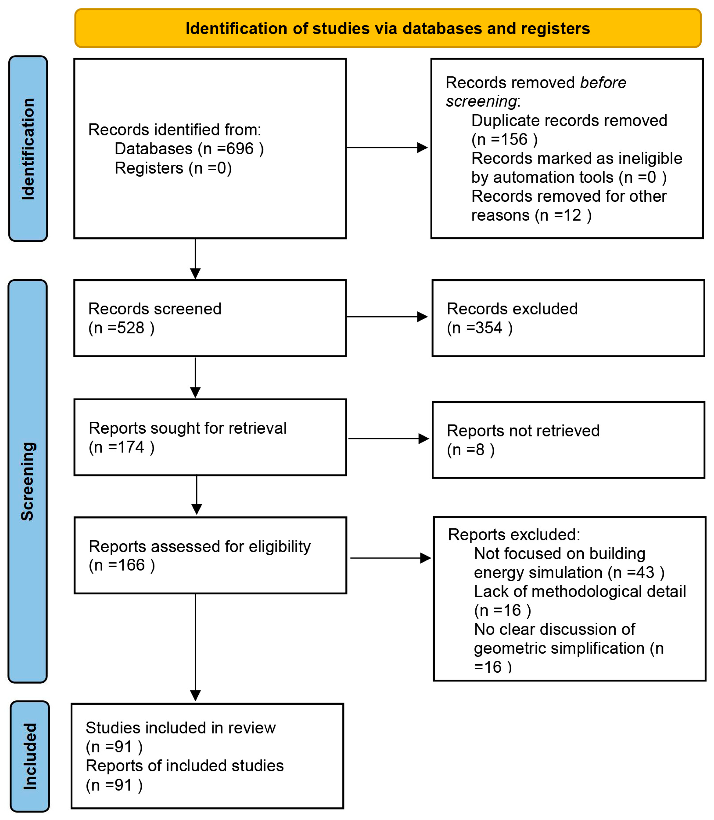
After removing duplicates and screening titles, abstracts, and full texts according to the relevance to the research scope, a total of 91 studies were retained for the final review. The overall study identification and selection process is presented in the PRISMA 2020 flow diagram (Figure 1). Due to the limited number of studies specifically addressing geometric simplification in historic building energy modeling, selected studies from modern building contexts were also included to provide methodological and conceptual references relevant to historic applications.

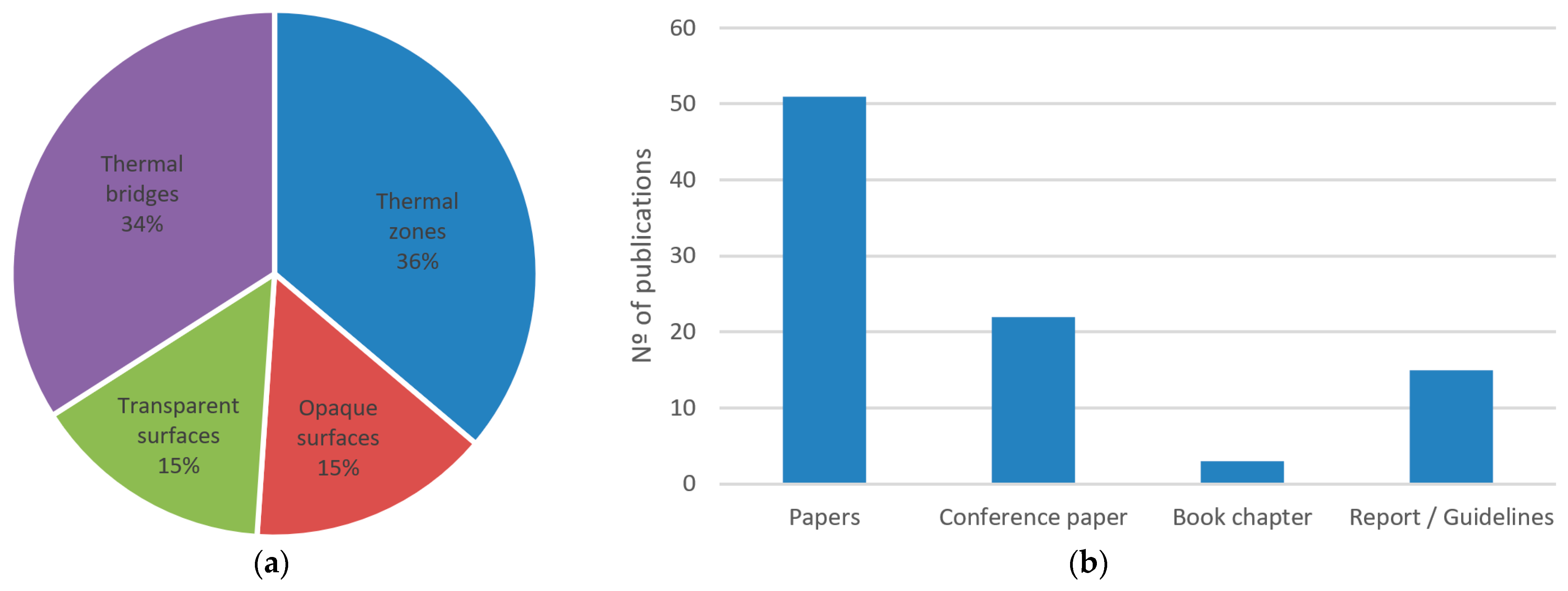
According to this review, the majority of the retrieved studies focus on simplification methods related to thermal zones (36%) and thermal bridges (34%), while fewer address opaque surfaces (15%) or transparent surfaces (15%) (Figure 2). In addition, Figure 2 summarizes the distribution of the reviewed literature by type of resource, showing that most contributions come from journal papers, with a smaller proportion from conference proceedings and technical reports/guidelines. This overview helps clarify both the relative emphasis of current research and the limited number of comprehensive studies on geometric simplification in the energy simulation of historic buildings.

The outcomes of this review should be regarded as an initial contribution toward establishing a structured methodology for geometric simplification in BES of historic buildings. Given the morphological complexity and heritage value of such structures, defining an appropriate level of geometric abstraction is both technically challenging and methodologically significant. Moreover, this review provides a foundational framework for the development of more advanced geometric simplification strategies adapted to different historic building typologies in future studies.

3. Review of Geometric Model Simplification in Energy Simulation Modelling

This chapter describes the main procedures for simplifying energy simulation models, evaluating different possibilities, and analyzing critical issues in the simplification procedures of thermal zones, opaque and transparent surfaces, and modeling thermal bridges. A detailed quantitative summary of the reviewed studies, including simplification methods, error ranges, and simulation impacts, is provided in

Table A1. Previous studies about geometric simplifications in building energy simulation.

Ref.	Building Information	Simulation Tool	Simplified Method	Indicator	Validation Results	What Did Literature Do?
[18]	House, Toronto (Canada)	Energyplus	S1: zoned by orientation; S2: zoned by above ground and basement; S3: single zone	Total energy demand	S1: −0.8%; S2: −11.4%; S3: −19.3%	Conducted sensitivity analyses to quantify the impact of thermal zoning on building performance.
[20]	Office building (2003) (US)	EnergyPlus	Koopman operator	Heating demand, Cooling demand	heating −2.7%, cooling −5.5%	Analyzed a detailed building energy model using an optimization method called the Koopman operator, to identify and develop zoning approximations based on zone temperature.
[14]	House (2012) (UK)	EnergyPlus	Zoned by floor	Heating demand, Simulation time	heating +10.6%, time −30%	Emphasized the benefit of simplified zoning models on reduced preparation and simulation time.
[19]	House (1960), Madrid (Spain)	TRNSYS	S1: zoned by orientation; S2: zoned by apartment; S3: zoned by floor; S4: three representative floors; S5: inside, center or outside perimeter	Heating demand, Cooling demand	S1: heating −3.9%, cooling −3.4%; S2: heating −10.2%; cooling −15.1%; S3: heating −12.5%; cooling −21.6%; S4: heating −14%; cooling +7.9% S5: 14% across heating, 10% across cooling	Investigated the effect of defining building’s geometrical and physical characteristics during the modelling phase on the assessment of building loads.
[15,31]	Office building (2007), Bolzano (Italy)	EnergyPlus	S1: zoned by floor; S2: three representative floors; S3: surface grouping; S4: zone squaring	Heating demand, Cooling demand	S1: heating −8.12%, cooling −9.29%; S2: heating −4.81%, cooling −7.86% S3: heating −1.43%, cooling −0.18%; S4: heating +1.35%, cooling +0.4%;	Analyzed detailed model and progressively simplified for: (a) accuracy through progressive simplifications, (b) most significant building parameters (c) maximum number of simplifications able to ensure time requirements in early-stage building design and acceptable correctness.
[17]	House and office building	EnergyPlus	Core and perimeter	EUI, Heating loads, Cooling loads	EUI: RMSE = 15%, Heating: RMSE = 175%, Cooling: RMSE = 105%	Compared results of 25 real floor plans corresponding to distinct morphologies obtained with detailed architectural zoning and with the perimeter and core zoning paradigm.
[21]	Office building (2007) (US)	EnergyPlus	Koopman operator	Heating demand, Cooling demand	heating −31.2%, cooling −9.1%	Introduced a systematic approach for creating zoning approximations in institutional buildings.
[16]	House (UK)	Designbuilder, EnergyPlus	S1: zoned by function and schedule; S2: zoned by floor; S3: zoned by building	Heating demand	S1: heating −6.9%; S2: heating −17.1%; S3: heating −26.1%	Investigated the effect of reducing the number of thermal zones in modeling a domestic building on prediction accuracy.
[22]	Office building	Revit, Energyplus	S1: Hierarchical clustering approach; S2: Koopman operator	Total energy demand	S1: −0.793%; S2: −0.815%	Evaluated two simulation-time reduction techniques in terms of their effectiveness to predict the energy demands under different retrofit scenarios.
[23]	House, Legnica (Poland)	Designbuilder, EnergyPlus	S1: zoned by schedule; S2: zoned by floor; S3: excluding shading elements	Heating demand, Maximum hourly power	S1: heating −2.4%, power +1.1%; S2: heating −8.3%, power +1.1%; S3: heating −3.5%, power +0.1%	Introduced different variants of the simulation model developed in DesignBuilder on the quality of results obtained to find simplifications which allow obtaining an acceptable level of deviations.
[25]	Office building, Kunshan (China)	EnergyPlus	S1: zoned by function, orientation and schedule; S2: zoned by floor; S3: surface grouping; S4: three representative floors; S5: inside, center or outside perimeter	Total energy demand, Simulation time	S1: energy +2.1%, time −8.2%; S2: energy +31.8%, time −32.1%; S3: energy +1.9%; S4: energy +3.1%; S5: 1.9% across energy	Investigated what the appropriate level of simplification in geometric modelling is.
[37]	Church (XIII century), Lisbon (Portugal)	WUFI Plus	S1: zoned by floor for additional functions; S2: surface grouping	Temperature and water-vapor pressure goodness of fit, Simulation time, Fit/Time	S1: fit(T) −1.5%, fit(Pv) −0.3%, time −15%, fit/time +14.3%; S2: fit(T) −1.7%, fit(Pv) −0.3%, time 0%, fit/time −2.3%	Evaluated model simplifications adopted for a historical building according to model’s accuracy/simulation time ratio.
[26]	House (2005), New Minia (Egypt)	IDA ICE	S1: zoned by function, orientation and schedule; S2: zoned by same oriented spaces for all floors; S3: zoned by floor; S4: zoned by building	Heating demand, Cooling demand, Simulation time	S1: heating −3.1%, cooling +9.6%, time −63%; S2: heating −3.5%, cooling +15.1%, time −84%; S3: heating −0.3%, cooling +10.6%, time −73%; S4: heating −23.6%, cooling +12.2%, time −94%	Simplified the model of a residence house in Egypt by incrementally reducing the number of thermal zones from modeling every space as a separate zone to modeling the building as a single zone.
[24]	High-rise residential building (South Korea)	TRNSYS	S1: no facility zone; S2: zoned by direct and indirect air conditioning; S3: zoned by air conditioned and unconditioned; S4: three representative floors; S5: five representative floors;	Heating and cooling demands, Heating and cooling peak, Simulation time	S1: cooling +0.83%, heating −0.77%, cooling peak +0.17%, heating peak −0.42%, time −15%; S2: cooling +12.08%, heating −1.1%, cooling peak +15.49%, heating peak +0.73%, time −35%; S3: cooling +13.08%, heating −2.32%, cooling peak +16.48%, heating peak −0.11%, time −38%; S4: cooling +12.43%, heating −1.75%, cooling peak +5.37%, heating peak −0.93%, time −83%; S5: cooling +1.96%, heating −0.18%, cooling peak +1.08%, heating peak −0.12%, time −75%	Conducted optimization of passive design strategy for residential buildings with building model simplification based on air conditioning to reduce the simulation time.
[32]	Office building (US)	EnergyPlus	1/2/3/6/12/60 representative floors	Annual energy intensity	across 0–0.69%	Studied the accuracy of using multipliers to reduce input data for building energy simulation.
[33]	Office buildings (Germany and Greece)	TRNSYS, Energyplus	S1: zoned by periodic geometries; S2: zoned by three sub-buildings	Simulation time, Temperature	S1: time −93.8%, temperature +16.7%; S2: time −81.2%, temperature +1.25%;	Highlighted the necessity of elaborate boundary conditions definition and showed the inability to provide efficient boundary conditions affecting its efficiency.
[36]	Exhibition hall (2015), Stuttgart (Germany)	Honeybee, Energyplus	Reduce low polygon mesh for curved surfaces	Total energy demand, Simulation time	energy: CVRMSE = 3.4%, NMBE = 0.1%	Presented a computational tool that automatically simplifies the geometry of complex curved building envelopes for energy simulation.
[34]	House (1989), Bergamo (Italy)	TRNSYS	Zone squaring	Total energy demand, Simulation time	energy −12%, time −50%	Defined a methodology aimed at the creation of a simplified energy model combined with heating plant simplifications.
[2]	Office buildings (circular and cross-shaped)	Honeybee, Energyplus	Reduce sides of planar for curved surfaces	Cooling load, Simulation time	cooling −1%, time −75%	Presented a comparison of different pathways for the energy modelling of complex building geometry.
[44]	Mansory building (1859), Ottawa (Canada)	Delphin	S1: 1-D blended model; S2: 2-D parallel model	Moisture gained, RHT Index	S1: gained −16.7%, RHT +167%; S2: gained +6.7%, RHT −25%	Examined how the variability in geometry and composition may affect model outcomes using a simulation approach with stochastic methods for a sample rubble core masonry wall.
[45]	House (14 C), Bolzano (Italy)	Delphin	S1: stone elements with different dimensions; S2: external regular stone blocks, different central stones; S3: external regular stone sides, different central stones; S4: only a central stone layer	Thermal conductance	S1: +5.8%; S2: +15.3%; S3: +18.2%; S4: +35.8%	Studied the influence of different geometrical simplifications, discretization, and material selections on the thermal performances of traditions stone walls.
[43,47]	Traditional solid wall	BuildDesk U, BRE U-value Calculator	S1: representation as two layers S2: a mortar core between two stone layers	U-value	S2 represents more accurately the higher presence of mortar within the core	Investigated the impact of traditionally constructed masonry wall on U-value calculations.
[46]	Ten historic buildings (12–18 C) (Italy)	-	S1: 90/10 stone to mortar; S2: 80/20 stone to mortar; S3: 86.6/8.7/4.7 stone to mortar and air	U-value	S1: 29–34%; S2: 24–29%; S3: 54–58%	Presented an interdisciplinary assessment methodology for the thermal performance evaluation of the traditional stone walls located in Lombardy Region.
[40]	House (17 C), Bolzano (Italy)	Energyplus	Homogeneous wall model	Indoor Air Temperature	RMSE = 0.66 K, MAE = 0.63 K	Proposed a calibration methodology aimed at reducing the risk of obtaining a calibrated model whose parameters are far from the actual values is particularly high in historical buildings.

in Appendix A.

3.1. Thermal Zones

A thermal zone consists of a building volume division into small zones used to perform more or less detailed calculations in building energy simulations. In the guidelines and regulations provided in different countries, several definitions of thermal zones exist.

Table 1. Overview of thermal zone division criteria as specified in various guides/regulations.

Guideline/Regulation	Definition of One Thermal Zone
BRE National Calculation Methodology modelling guide [9]	“A thermal zone is an area that: a. Has the same heating and cooling set-points; b. The same ventilation provisions; c. Has the same plant operating times; d. Has the same set-back conditions; e. Is served by the same type(s) of terminal device; f. Is served by the same primary plant; g. Where the output of each type of terminal device is controlled in a similar manner.”
The Canadian standardization method EE4 [10]	“A thermal zone, generally referred to as a zone, are portions of a building served by a common HVAC system that have similar heating loads, cooling loads and operating schedules.”
ASHRAE 90.1 [11]	“Different HVAC zones may be combined to create a single thermal block or identical thermal blocks to which multipliers are applied provided all of the following conditions are met: a. The space use classification is the same throughout the thermal block. b. All HVAC zones in the thermal block that are adjacent to glazed exterior walls face the same orientation or their orientations vary by less than 45 degrees of each other. c. All of the zones are served by the same HVAC system. d. All of the zones have schedules that differ by 40 or less equivalent full-load hours per week.”
Commercial Energy Services Network (COMNET) [12]	“A thermal block is a space or collection of spaces within a building having sufficiently similar space conditioning requirements so that those conditions could be maintained with a single thermal controlling device. A thermal block is a thermal and not a geometric concept: spaces need not be contiguous to be combined within a single thermal block.”

provides an overview of thermal zone (or thermal block) definitions based on different criteria, including usage, temperature control, solar gain, perimeter or interior location, HVAC distribution system type, and separate interior and perimeter thermal zones.

As provided in Table 1, the thermal zone divisions are largely similar; however, in practical modeling, these guidelines often lack precise direction, leaving energy simulators to rely heavily on their personal experience. Therefore, more practical simplification methodologies need to be studied further, and can be divided into grouping of thermal zones, the use of the inside, center or outside perimeter for the size definition, construction of part or all of the building, and irregular shapes. As the thermal zoning process is a pivotal step for both simulation accuracy and workflow efficiency, the following sections discuss some critical aspects in the definition of thermal zones and provide recommendations for the proper modeling of historic BES models.

3.1.1. Grouping of Thermal Zones

In building energy simulation, grouping of thermal zones is an effective method to simplify model complexity and reduce workload. Merging thermal zones with similar thermal characteristics, usage patterns, or load profiles into a single group helps lower computational time and resources while preserving accuracy [13]. Thermal zone grouping is particularly suitable for large buildings, preliminary design stages, or when optimizing computational efficiency. Given the few studies focusing on thermal zone grouping in historic building energy modeling, this section critically reviews relevant research from modern contexts. While historic structures often present more complex and irregular spatial configurations, understanding how zone aggregation impacts simulation accuracy in modern contexts provides a valuable theoretical foundation. These approaches offer transferable insights that can guide the development of adaptation strategies tailored to the morphological and functional characteristics of historic architecture. Therefore, despite the contextual differences, these methods are reviewed here for their potential applicability and for highlighting gaps in current historic building research.

In this regard, several studies have examined how thermal zone grouping affects the accuracy of results. For example, Korolija et al. [14], Picco et al. [15] compared the detailed model in which one zone per room with a simplified model in which one zone per floor, finding that the simulation time could be reduced by 30% with the annual heating demand underestimated by around 14%.

Heo et al. [16] studied a semi-detached UK house and found that reducing zones to one per floor or one for the entire house led to heating demand underestimations of 17% and 26%, respectively. Dogan et al. [17] compared detailed zoning with the perimeter and core zoning defined in the ASHRAE 90.1 on 25 real floor plans corresponding to distinct morphologies, reporting large variations in energy use intensity and inconsistencies in energy load predictions.

The above studies show that the thermal zone grouping can significantly reduce simulation time, while oversimplification may compromise accuracy [18]. Therefore, many researchers focus on further improving the prediction accuracy of grouped thermal zones. Dipasquale et al. [19] divided the thermal zones by apartment and further by orientation (north and south). The output results showed that these two methods underestimated the heating demand by 10.2% and 3.9%, respectively. Georgescu et al. [20,21] used the Koopman operator to reduce a 191-zone model to 32 zones, with only a 3.3% error in annual heating and cooling load prediction. Similarly, Giannakis et al. [22] proposed hierarchical clustering approach, in which the thermal zones were merged iteratively. However, both methods require a fully detailed baseline model, which can be time-consuming and introduce uncertainties. Klimczak et al. [23] grouped the thermal zones based on their operating temperature, concluding that merging zones with similar internal conditions can simplify models while preserving reliability.

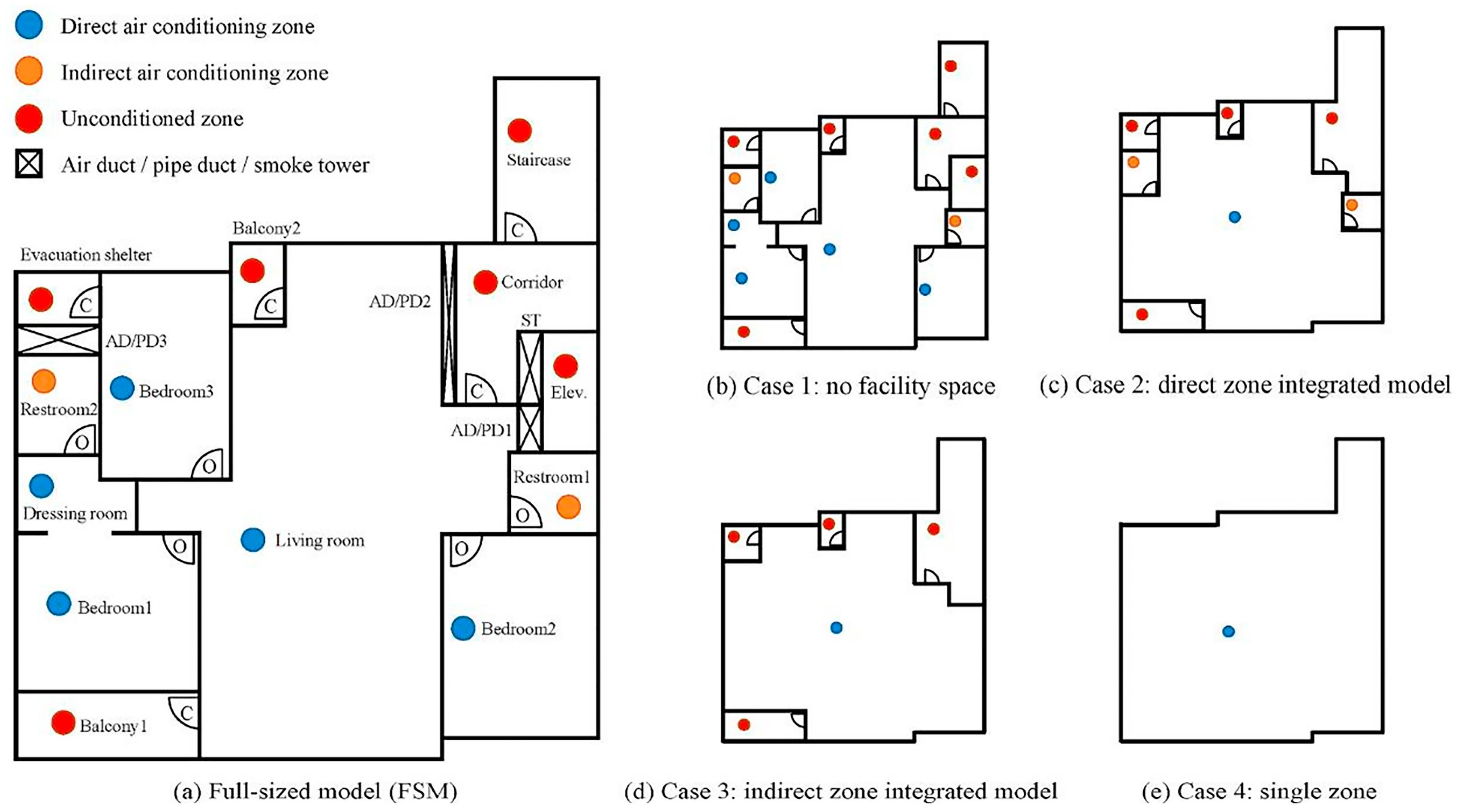
In addition, Jung et al. [24] divided the thermal zones into direct air conditioning zone, indirect air conditioning zone (i.e., a space that is not mechanically conditioned but whose temperature is influenced by adjacent directly conditioned zones, such as restrooms) and unconditioned zone, and finally tried to merge them (Figure 3). The result showed a different trend, particularly regarding cooling demand, which can be explained by the coupled air flow due to the integration of the direct air conditioning zone. The full-sized model had a slow coupling air velocity, while the integrated zone had a relatively fast coupling air velocity.

Furthermore, some studies try to summarize guidelines for maintaining model accuracy. In the research of Georgescu et al. [20,21], some guidelines are proposed, including the following: (1) when merging zones, the thermal mass of unmodeled walls should be captured; (2) zones containing exterior surfaces should not be merged with zones that do not contain exterior surfaces; (3) perimeter zones that are merged should have similar surface orientations and window areas; and (4) zones with small volumes and surface areas can be merged with much larger adjacent zones with little loss of accuracy.

Zhao et al. [25] defined the division of thermal zones based on the above-mentioned national standardization methods. They defined a thermal zone as one with the following characteristics: (1) spaces in a thermal zone must be on the same level in the building; (2) the orientation of the exterior walls of the spaces in a thermal zone is the same or their orientation difference is less than 45 degrees; (3) the surrounding space (walls in this space are exposed to the air) and internal space should be divided into different thermal zones; and (4) the heating and ventilation systems and temperature setpoints of these spaces should be the same. Using this approach for an office building, the annual energy demand was only overestimated by 2.1%, and the simulation time was reduced by 8.2%, compared with the detailed model. Elhadad et al. [26] used similar criteria considering orientation, operation schedules, use, etc. The cooling demand increased by 9.6%, the heating demand decreased by 3.1%, and the simulation time decreased by 63%. They emphasized that differently oriented zones should not be combined to avoid different solar heat load (summer) or heat gain (winter) effects being mixed in one greater unified zone to confuse both energy and comfort behavior.

D. Bishop et al. [27] investigated three zoning strategies in a New Zealand residence. In the first strategy, which is the most detailed, a thermal zone for each room has been created; in the second, two thermal zones have been created based on the conditioned and unconditioned spaces, while in the third, a single thermal zone has been created for the whole building. The results showed that in the second and third zoning definitions, the percentage error in predicting the peak heating power, with respect to the first zoning definition, increased between −0.6% and −3.1% for the second and between −2.4% and 5.0% for the third strategy. The authors stated that such underestimation is probably due to the moderating effect of larger zone air volumes, which dampen the rate of exchange of temperature.

3.1.2. Inside, Center or Outside Perimeter

Energy simulation software typically does not require the inclusion of envelope thickness in the modeling process. In determining the position of a building’s exterior walls, energy modelers often use the internal, external edge, or center line dimensions (Figure 4). Modeling based on the external edge allows for a more accurate simulation of outdoor solar radiation and heat gains, while overestimates the volume, using the internal edge ensures accurate calculations of the building area and interior room volume, while underestimates the dispersion losses, and the center line is in between the previous solutions. This issue is particularly critical for historic buildings, where wall thickness can be substantial. In such cases, adopting the external edge may significantly overestimate the conditioned volume, while relying on the internal edge may distort the actual building geometry, leading to inaccuracies in thermal mass and envelope area estimation.

In the literature, Dipasquale et al. [19] explored how different building size definitions affect energy performance. Among the three methods, the second method resulted in a 14% higher simulated heating demand and a 7.2% higher cooling demand compared to the first method. The third method led to an even greater increase, with heating demand rising by 16.1% and cooling demand by 9.8%. They thought the difference was mainly due to the influence of solar gains and proposed to use internal cold bridges to reduce the difference. Zhao et al. [25] also tried to carry out comparisons between three methods, in which the energy demand by using the second and third methods increased by 2.5% and 1.8%, respectively, compared to the first one.

Ladenhauf et al. [28,29] proposed an algorithm for the geometric simplification of the complex building information models according to semantic constraints to create simple building models for energy analysis. Building geometries are reduced to flat surfaces without thickness representing the thermal shell, with outer edges used for exterior elements and centerlines for interior ones.

As suggested in the “Tips and Tricks for Using EnergyPlus” document [30], a suggested approach is to consider outside dimensions for exterior surfaces and centerline dimensions for the interior surfaces in order to properly calculate the floor area, zone volume, and thermal mass. Moreover, the document highlighted that only in buildings with huge thick walls (as in historic buildings), it is recommended to use the centerline dimensions for all surfaces (exterior and interior) to properly consider the given thermal mass, without excessively overestimating the volume.

3.1.3. Construction of Part or All of the Building

When establishing a geometric model, it is common to simplify buildings with typical floors, which have consistent spatial layouts and thermal characteristics, by modeling only one representative floor. For buildings with several floor levels, modelers often simulate the ground floor, top floor, and a single middle floor, with the results extrapolated accordingly. This method is supported by tools such as EnergyPlus and eQuest, although it is not explicitly mandated by national simulation standards and is primarily outlined in software user manuals. In historic buildings, however, this approach must be applied with caution. Many heritage structures lack standardized floor repetition, as their vertical spatial organization often varies significantly in height, layout, and function. That said, certain sections, particularly former residential areas, may display some degree of repetition, in which case simplified floor-based modeling can be cautiously adopted, provided the spatial and functional consistency is verified.

In the research of Picco et al. [31], they tried to simplify a six-story office building in Italy by modeling just three zones (or floors), one for the underground deposit, one for the top floor, and one for the middle floors. The heating and cooling energy demand were underestimated by 4.8% and 7.9%, respectively. Ellis et al. [32] studied the accuracy of using multipliers to reduce input data and concluded that even simulating a single floor with a multiplier could give accurate annual energy results for an entire building, as long as the floor to be simulated is near mid-height. Although accurate for the whole building, the results may not accurately predict the performance of a specific floor. This result has potential implications for HVAC equipment sizing. Dipasquale et al. [19] compared the simplified method of the number of floors with the staircase modeled with a single air-node zone and a multi-air-node zone (Figure 5). They found that multi-node models, which account for long-wave radiation reflections and air temperature stratification, better represent building behavior and may be preferable in similar cases.

Jung et al. [24] simplified the model of a 19-story high-rise residential building into 3, 5, 7, and 9 stories. Compared with modeling three floors, more floors captured the temperature gradient better. For example, in the case of a seven-story building, the result considered not only the value of the ground, middle and attic floors but also the value of the upper floor of the ground floor and the lower floor of the attic floor. While accuracy decreased slightly with more simplification, computational time improved significantly.

Besides the modeling of typical floors, geometric simplification can also be achieved through the construction of the representative building block. In this regard, Giannakis et al. [33] presented two techniques: one is the geometry simplification for periodic geometries, and the other is the use of co-simulation to split a building into simpler sub-buildings, which can be evaluated in parallel and exchange boundary conditions data during simulation. While geometry simplification had difficulty defining accurate boundary conditions, the co-simulation approach seems more effective, since its implementation reduced runtime by up to 80% and preserved boundary accuracy.

3.1.4. Irregular Shapes

In building energy simulation, irregular shapes, such as curved surfaces, special-shaped structures, asymmetric layouts, etc., become difficult to model due to their complex geometric features, and their dynamic thermal performance is significantly different from that of regular shapes. In historic buildings, irregular shapes are particularly prevalent, reflecting traditional construction methods, successive modifications, and stylistic features from different historical periods. Elements such as curved vaults and asymmetrical floor plans are typical features of heritage structures and pose significant challenges for accurate geometric representation. Therefore, existing simplification approaches originally developed for modern non-standard architecture may offer methodological insights but require careful adaptation to address the unique geometric and material characteristics of historic buildings.

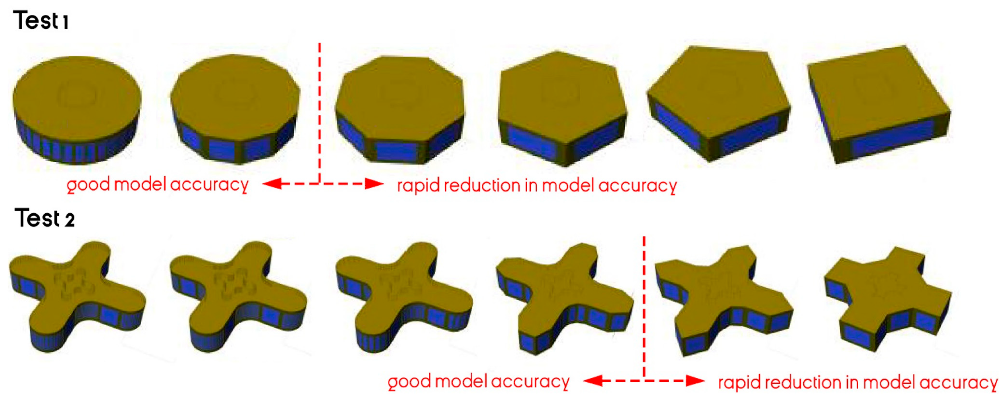
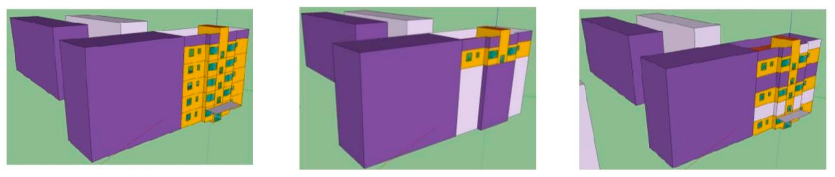
For buildings with irregular shapes or some auxiliary spaces outside the main shape, simplifying the building shape is often necessary to improve simulation efficiency. In historic building energy models, Akkurt et al. [4] concluded that the simplification of geometry is often unavoidable for use in building-energy performance simulation, but inaccuracies resulting from oversimplification in some geometrical characteristics must be avoided. Picco et al. [31] researched zone squaring, where complex zones are approximated as rectangular boxes. To minimize the differences, they compared three kinds of zone floor areas, which characterized all internal gains and air changes. The floor area equal to the area of the box generated by vertical surfaces made a larger difference, while the floor area equal to the mean floor area of the building and specified for each floor provided a closer result. The second method required significantly less input data, which was more suitable. However, the applicability and accuracy of such simplification approaches may also depend strongly on the architectural and constructive characteristics of buildings. In many historic buildings, floor areas and internal layouts vary significantly between levels despite having similar external façades, due to differences in wall thicknesses, structural systems, vaulted spaces, or floor-specific spatial organizations. Such irregularities may increase the uncertainty associated with simplified zoning approaches. Alberto Beltrami et al. [34] applied the same simplification method to a residential unit in Italy and combined it with heating plant simplifications. The most simplified dynamic simulation showed up to 12% loss in accuracy, but reduced simulation time by 50%, equating it to a stationary simulation. However, the latter lacks the benefits of dynamic control of HVAC systems under varying conditions. Chatzivasileiadi et al. [35] examined the impact of simplifying complex building geometry on the accuracy of BES. Through a literature review and systematic test cases (shown in Figure 6), the study finds that geometry can often be simplified significantly without major loss in accuracy or increased simulation run time. However, accuracy drops sharply beyond a certain threshold. For example, simplifications in circular-plan and cruciform showed deviations ranging from about 3.2% to 9%. The study concludes that while model simplification is beneficial to reduce the computational efforts and simulation run time, excessive simplification, especially using orthogonal prisms, can cause a noticeable decrease in model accuracy.

Similarly, Santos et al. [36] simplified complex curved surfaces of a building envelope by generating low-polygon meshes, inspired by the Exhibition Hall pavilion. They found an exponential relationship between simulation run time and geometric complexity. High levels of geometric simplification might fail in fully capturing solar-related phenomena such as solar heat gains and daylighting. As a result, they recommended limiting polygon reduction to 80% of the original surface detail. In another study [37], the authors tried to simplify the modeling of a historic church in Portugal to reduce simulation time for sensitivity analysis. They aligned the main door with the facade and finally achieved a higher accuracy/simulation time ratio.

3.2. Opaque Surfaces

As the main body of the building envelope (such as walls, roofs, floors, etc.), opaque surfaces undertake the comprehensive functions of heat conduction, heat storage, insulation and geometric simplification in energy simulation directly affects the accuracy of building thermal inertia, heating and cooling loads, as well as the energy consumption. Heat losses through the opaque surfaces often play a significant role in the energy balance of the building, although the relative contribution of opaque and transparent elements may vary depending on the thermal performance of the building envelope [38]. Unlike transparent surfaces, opaque elements do not transmit light, but their nonlinear heat transfer and multi-layer composition (e.g., insulation, finishing and structural layers) require careful modeling. This aspect mainly happens to historic buildings since the main geometrical features are related to irregular and complex shapes (e.g., vaults, arches, tapered walls, moldings, ornament al parts), and variable thickness of walls and ceilings (in some cases also due to damage problems) [4]. Despite this complexity, in many related studies [8,39], a simplification of geometry and the assumption of an average wall thickness is considered as an acceptable approximation.

3.2.1. Non-Homogeneous Stratigraphies

Non-homogeneous stratigraphies are building components composed of mixed or layered materials with spatially uneven distribution of physical properties (e.g., thermal conductivity, density, porosity). Such structures are often found in walls, roofs, or floors of historic buildings, with variable thicknesses and different levels of decay along the perimeter and across the height of the building, such as masonry walls, wooden frames with stucco infill, etc. The uncertainty in material composition and properties increases the difficulty of assigning reliable thermophysical parameters in simulation models.

In a study [40] where irregularities due to changes in material thickness and properties exist, the mean wall thickness in the building model has been considered an acceptable approximation. In particular, Roberti et al. [40] used the average thickness and the thermal properties of the predominant material for each of these components of a XIII century building, and key parameters were calibrated through sensitivity analysis. However, the authors highlighted that this kind of simplification can work specifically for the case study under analysis. Moreover, they stated that the oversimplification of the thickness, thermal capacity, and properties of the building envelope may significantly affect the time shift and weekly peaks of the simulated temperatures.

In this regard, previous studies have pointed out the discrepancy between in situ measured and calculated thermal properties [41,42,43] and the lack of guidance on how to incorporate such aspects into the simulation model [41].

For instance, Michael Gutland et al. [44] examine how the variability in geometry and composition may affect simulation outcomes by using stochastic methods to create the geometry for a sample masonry wall. In this work, the stochastic model has been compared with simplified 1D and 2D components, where some of them were made through the “blended materials approach”. In particular, it is a simplified process that consists of creating stone/mortar layers with hygrothermal properties calculated by the weighted averages of the percentages of composition of stone, mortar and air. The following formula has been used for the calculation of the conductivity, but also for the other parameters (such as density, specific heat, porosity, etc.):

$${\mathsf{\lambda }}_{\mathrm{blended}}={\%}_{\mathrm{stone}}·{\mathsf{\lambda }}_{\mathrm{stone}}+{\%}_{\mathrm{mortar}}·{\mathsf{\lambda }}_{\mathrm{mortar}}+{\%}_{\mathrm{air}}·{\mathsf{\lambda }}_{\mathrm{air}}$$

(1)

This simplified weighted-average approach assumes a relatively homogeneous distribution of stone, mortar, and air within the wall section and neglects local heterogeneities, directional heat transfer effects, and complex void distributions. Therefore, its reliability may decrease for highly irregular historic masonry walls characterized by large voids, non-uniform material arrangements, or significant moisture-related effects.

It should be noted that the different percentages of stone, mortar and air might be assumed according to a survey or other information collected. According to the work [44], it was found that the 2D approach (which takes into account also the mortar joints) was the most appropriate for the specific type of wall analyzed, but had difficulties in accurately accounting for the voids. However, stochastically generated geometries required too much effort to be produced and time to be simulated.

In another work [45], the authors analyze the influence of different geometrical simplifications, discretization and material selection on the thermal performances of a traditional stone wall with an irregular ashlar exterior and mixed-material core. In that case, the geometry of the wall was simplified into four layouts with different levels of detail and the calculation of thermal conductance was compared with in situ measurements (made through a heat flux meter) to evaluate the accuracy of the different layouts. The analysis shows that improving the level of detail of the model allows for providing more reliable results. In this regard, the authors highlight that retrofit intervention based on an incorrect evaluation of the building component might cause disadvantages for the building and possible legal claims. In a technical report [43], a variety of walls made of rubble core and cavities under real and laboratory conditions have been examined. It has been found that the calculation of the U-value based on software and standard material information usually overestimates the measured U-value of traditional walls [43,46]. Therefore, traditional building elements tend to perform better than would be expected from the U-value calculations. More in detail, the simplification process adopted to simulate the existing wall consists of the creation of a multi-layer component with the same proportion of stone, mortar, and voids of the real element, which should be known or assumed. The example shown hereafter (Figure 7) represents a rubble wall with 60% stone and 40% mortar, which can be modeled as two or three layers representing the correct proportions of the materials.

It should be noted that the number of layers and their position can significantly affect the hygrothermal simulation. Moreover, such layered simplification also influences the representation of the wall’s thermal inertia, as the distribution and specific heat capacity of each layer determine the wall’s ability to store and release heat over time. Inaccurate layering may therefore lead to unrealistic thermal buffering effects, particularly in heritage constructions characterized by heterogeneous and massive wall assemblies. Therefore, these aspects should be properly evaluated case by case according to the scheme that best represents the real condition. In this study [47], the author stated that the three-layer simplification scheme shown in Figure 7, consisting of two outer stone layers and a central mortar layer, although still very simple, represents more accurately the higher presence of mortar within the core of the traditional stonewall construction.

Finally, the authors stated that to better model such a type of wall, more information about the construction details is required [43], including the following:

• the thickness of layers;
• status of cavities, such as insulated/uninsulated and ventilated/unventilated;
• ratio and types of stone, mortar and voids;
• thermal properties of materials used in traditional construction.

Furthermore, they recommended further research and in situ measurements to define a more accurate U-value and to provide a more accurate thermal/energy assessment of existing buildings. Such investigations may include heat flow meter measurements [48], infrared thermography [49], wall probing and masonry stratigraphy investigations [50], as well as low-destructive or non-destructive testing techniques for identifying material properties in historic buildings [4].

Elena Lucchi [46] analyses the thermal performance of existing masonry walls through the comparison of analytical calculations of the U-value and in situ measurements. Such work confirms that the analytical calculation usually overestimates the U-value, due to the conservative data of the database adopted. Moreover, the author highlights that when the U-value is calculated, the percentage of the stone, mortar and voids that might affect the results is usually not considered. In such regard, the author suggests a range of proportions for rubble stonewalls in the Lombardy Region, which could be about 80–85% for stone, 13.5–16% for mortar, and 1.5–4% for air. Finally, the author recommends that it is preferable to adjust U-value calculations based on material composition rather than treating walls as homogeneous layers, particularly in thinner walls where such effects are more pronounced.

3.2.2. Surface Irregularities

Surface irregularities refer to structures in historic buildings that do not conform to modern standardized geometric forms, including special-shaped components, battlements, decorative elements, etc. Such forms are commonly seen in church domes, arcades, carved cornices, etc., and are typical features of cultural heritage, but they can bring significant challenges to energy and hygroscopic simulation modeling. Despite their possible impact on the results, few studies have explicitly addressed this issue within the context of building performance simulation.

In the research of Klimczak et al. [23], they excluded the shading elements as a step in the simplification of the energy model. The authors show that in the case where the shading elements affect the north-facing side, their exclusion would not have a significant impact on energy demand, while in the case where the elements affect the south-facing side, a considerable influence is given in the output, therefore, this simplification should not be applied.

In a historic palace located in Bologna (Italy) [51], which is characterized by massive battlements, the authors modeled these complex architectural elements as shading surfaces. To simplify the simulation, the thermal mass of the battlements was neglected based on the assumption of a high ventilation rate in the adjacent walkway, which was considered sufficient to equalize the surface temperature of the battlements with that of the external air.

It should be noted that further examples concerning the influence on simulation output due to point elements present on the envelope surfaces might be closely related to the effects of thermal bridges. Therefore, for a more detailed discussion on how to consider these aspects in the simulation model, see Section 3.4.

3.3. Transparent Surfaces

Transparent elements in buildings are generally windows, skylights, glazed surfaces of opaque doors, and glass blocks [52]. In historic buildings, transparent elements, particularly windows, often possess distinct morphological and material characteristics compared to those in modern architecture. Their dimensions, placement, frame-to-glass ratios, and glazing types are frequently determined by aesthetic, structural, and historic considerations rather than by performance-driven criteria. As a result, accurately modeling these elements is especially critical when simulating historic buildings, where simplification decisions may significantly impact the reliability of energy, lighting, and comfort predictions.

3.3.1. Surfaces Grouping

Windows are a critical component of the building envelope. The input of the window in energy simulation is mainly divided into two steps: geometric placement and thermal parameter input. For the latter step, some recommendations are already provided in the work carried out by the IEA-SHC Task 59 [4]. Furthermore, if the windows have sections with distinct thermal properties, this must be considered during the modeling process. Otherwise, for more complex cases (e.g., stained glass windows decorated with painting technique), instead of considering an average value of the glazing properties, such as the Solar Heat Gain Coefficient (SHGC) and Visible Transmittance (Vt), a sensitivity analysis is recommended to identify the most accurate input values [37].

This section focuses on the first step. For the simplification of windows in the geometric modeling phase, ASHRAE 90.1 [11] suggests merging all windows on the same wall within a thermal zone into a single window with equivalent area, when internal sunlight distribution is not critical [53]. It should be noted that ASHRAE 90.1 excludes historic buildings from several requirements, and therefore these recommendations should be considered with caution when applied to historic contexts. There are also relevant operational suggestions in the software usage tutorials, such as EnergyPlus 9.6. However, a notable drawback of this method is that window frames are typically not considered. This omission can lead to two important issues, e.g., an underestimation of thermal losses, as frame materials often have lower thermal performance than glazing, and an underestimation of solar gains, since frames reduce the effective glazed area. This issue is particularly relevant in the modeling of historic buildings, where window design and proportions often differ significantly from contemporary standards.

Picco et al. [31] analyzed the maximum simplifications in the early stage of building design with acceptable correctness. During the modeling of the windows, every single surface was modeled with the total area of all transparent surfaces of the complete model. Considering the reference fenestration height, there were two data inputs (total area and height) for each surface and eight inputs for each floor (total area and height in the four building vertical plane directions). As a result, the heating energy demand was underestimated by 1.43% and the cooling by 2.09%.

In addition, Zhao et al. [25] merged all the windows in one wall of the same thermal zone into one window. The energy demand was overestimated by 1.9% due to a change in the solar heat gain of the corresponding thermal zone after the change of window positions. In their opinion, this change would be more pronounced with external obstructions.

In other work [27], four different window simplifications have been tested. In particular, windows have been analyzed from a detailed modeling, which considers the real windows’ position, size and includes the border of the wall to a rough modeling which considers a single window centered in the wall surface and which does not consider the wall border shades. In this case, the authors highlight that grouping all windows into one had the largest impact. Such results indicate that shading/window interactions are key drivers of error, particularly for annual heating load (−3.8%) and overheating (11.1%). An accurate modeling of window placement is essential where those assessments are critical and where there are obstructions near windows (eaves, trees, closely neighboring buildings, etc.).

3.3.2. Window Frames, Glazing Area Partitioning and Window Position

Historic windows come in a variety of shapes and sizes. In modern buildings, the windows are typically square or rectangular, making them easily modeled with BES. However, windows found in churches, castles, and other distinctive structures often feature circular, mullioned, or irregular designs. Accurately modeling these windows could be challenging due to the missing information about the material properties and, in particular, the required geometric and structural simplifications considering window frames [4]. Furthermore, generally historic buildings are characterized by thick walls that might affect the energy balance of windows, reducing the amount of solar radiation. Such aspects, which are typically neglected, in some cases, could consistently affect the results in BES.

In detail, the effect of the thickness of the walls on windows might have a more or less pronounced impact on simulation results, in terms of heating and/or cooling energy demand, depending on window position, orientation, building location, etc. In historic building energy modeling, this aspect could be emphasized since they are often characterized by thicker walls with respect to modern construction. In this regard, a work [27] which assesses the impact of different levels of detail on energy modeling, emphasizes how important it is to realize the shading elements in order to obtain accurate results [27]. The authors point out that the impact of wall thickness can be almost negligible in some cases, while in others it can have a relevant effect. Therefore, it is necessary to consider on a case-by-case basis what level of detail to assume when building a model and the goal of the assessment.

A further and common simplification procedure involves creating the geometry of the entire window without considering the frame, assuming the window surface to be fully glazed. While this approach may slightly affect the thermophysical properties, a study [54] found only a 0.67% difference in energy use between models with and without frames for a simple rectangular window. Therefore, the authors conclude that modeling only the glazed part without considering the frame provides a negligible error in the final outcomes. However, it should be noted that such results are based only on a simple rectangular-shaped window with a single vertical partition in the middle.

The simplified process usually adopted by energy simulation software, which considers only a few parameters to define the performance of a window system (such as the overall U-value of the window, SHGC and Vt), could provide less accurate results, as depicted by some authors [55,56]. In particular, D. Arasteh et al. [55] pointed out that with the simplified approach, usually a full window with frame, partitioning, etc. and a fully glazed window, with the same above-mentioned characteristics, will provide the same annual energy results because their inputs are the same. However, as depicted by the authors, a more detailed analysis would produce different results in terms of annual energy needs and peak loads. In this respect, a work done by M. Thalfeldt et al. [56] has shown that in cold climates, detailed modeling of the window system provides higher heat losses and lower cooling needs than simplified models. Such a difference is mainly due to the simplification made in the calculation of solar gains and the use of a constant U-value through simplified window models. In particular, the heating and cooling energy demand is about 7% and 23% respectively between the simplified and detailed energy models, considering the specific building components.

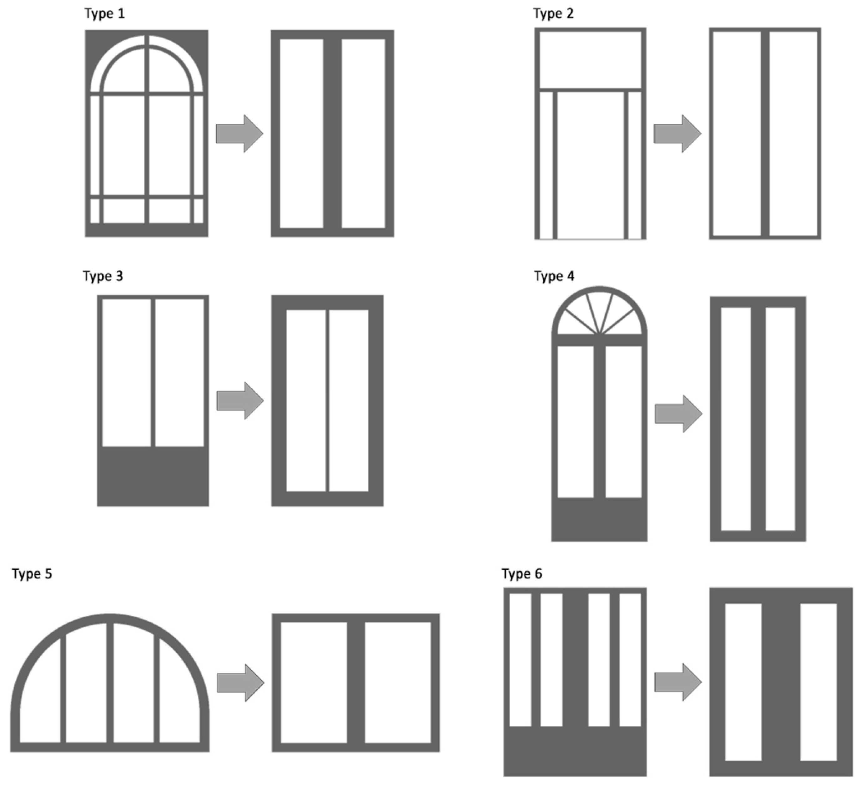
In a recent work done by G. Evola et al. [57], where the complex windows and doors typologies have been simplified through a geometrical process that transforms the real shape of the openings into a rectangular element, maintaining the real glass and frame areas (Figure 8). Such an approach, as highlighted by the authors, allows an accurate estimation of the solar gains through these elements, which is particularly important in Mediterranean areas. In the following figure, some examples of the geometrical simplification process of the window and door systems are shown.

Within energy simulation software, an approach [58] to accurately take into account the window frames and dividers is to use software such as WINDOW 5. Such tools allow a precise evaluation of direct and diffuse solar radiation absorbed by the outside and inside frame surfaces, the calculation of the shadows of the framing onto the glass, and the effect of the thermal bridge across between-pane spacers. In this case, the detailed information provided in the software can be imported into the energy model to be used in the heat balance calculations. It should be noted that such an approach requires detailed information on the window elements, a higher simulation run time, and user experience with respect to the simplified procedure, however, it could provide more reliable results.

Alternatively, if a detailed analysis of the window element is required, as suggested by some authors [59], the calculation of the whole window thermal transmittance is usually done in three major steps: calculation of center of glazing values with 1D models, calculation of multi-dimensional and frame effects on window/frame components (usually with 2D thermal simulations), and finally the combination of glazing and frame component results. Each step of these calculations is supported by standards [59].

3.4. Thermal Bridges

A significant part of heat loss in a building can be attributed to thermal bridges, which occur where the continuity of thermal resistance in the envelope is disrupted—typically at junctions between walls, floors, and ceilings. Thermal bridges are generally classified into two types: linear thermal bridges, defined by a linear thermal transmittance (Ψ) and occurring along lines such as wall intersections; and punctual thermal bridges, defined by a point thermal transmittance (χ) and typically found at singular junctions, such as at local fixing systems [60].

According to different sources, the impact of thermal bridges on the energy demand of dwellings can range from 5% to 39% [61], particularly if the insulation level of the envelope grows (for example, in highly insulated single-family houses with bad thermal bridge treatment). In addition, a thermal bridge can lead to local discomfort (cold wall, mold, soiling, etc.) [62]. In historic buildings, addressing thermal bridges is particularly challenging due to irregular geometries, thick masonry, and non-standard connections. Moreover, due to the typically low airtightness and high thermal mass of such structures, some studies suggest that thermal bridges may have a limited impact on overall energy performance and indoor air exchanges [53]. However, this assumption remains debated, and the role of thermal bridges in historic envelopes requires careful evaluation, particularly when pursuing energy retrofit interventions or hygrothermal risk assessments.

3.4.1. Existing Methods for the Evaluation of Thermal Bridges in Energy Simulation

In many European Union countries, the assessment of thermal bridges in energy simulation is mainly conducted using procedures that are based on standards (e.g., EN ISO 14683 [63] and EN ISO 10211 [64]) or abacus/catalogues (e.g., CENED in Italy [65], the “Catalogue des ponts thermiques” in Switzerland [66], etc.).

In the literature, simplified and detailed approaches can be distinguished [65]. The first ones are generally more practical and computationally efficient, but often rely on steady-state assumptions and standardized values from abacus/catalogues, which can result in inaccuracies for non-standard constructions such as historic buildings [67]. Some models assume uniform thermal inertia between bridges and adjacent walls or adjust the overall U-value to account for added losses. Others apply correction factors or modify thermal capacity values, but such 1D methods generally fail to capture the multidimensional nature of heat transfer at junctions.

In contrast, detailed methods offer higher accuracy by explicitly modeling the complex multidimensional (2D or 3D) heat flow and the dynamic thermal behavior of thermal bridges. Although computationally demanding, they are indispensable for realistic energy assessments, as they capture thermal inertia effects that steady-state methods overlook. Numerical techniques, such as the Finite Difference Method (FDM), Finite Element Method (FEM), or Finite Volume Method (FVM) are commonly employed. Standards like EN ISO 10211 and EN ISO 14683 formalize the use of the linear thermal transmittance, derived from 2D calculations, but these are often applied as static inputs in dynamic simulations, potentially reducing accuracy.

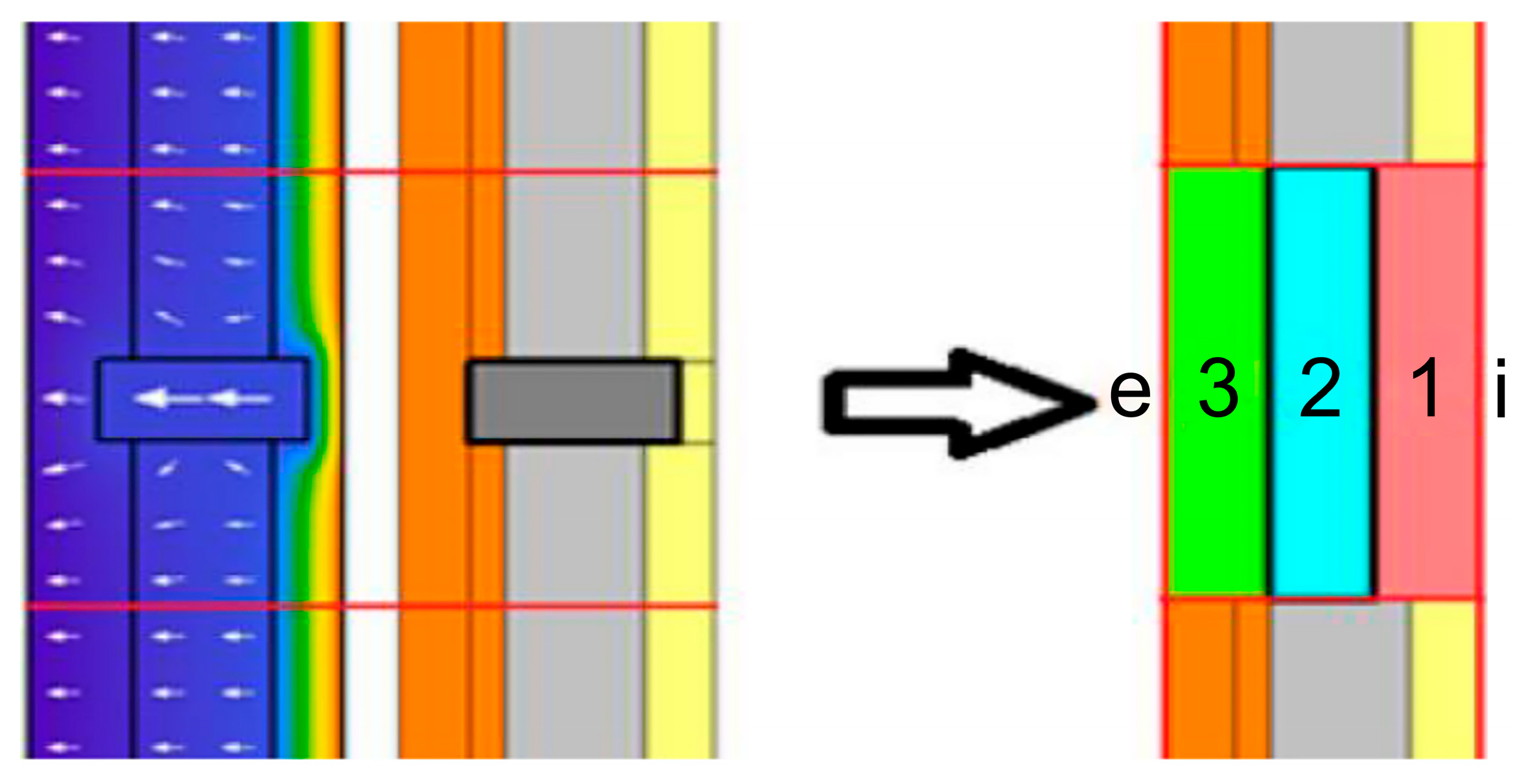
In such regard, several dynamic methods have been developed to account for thermal bridges, notably the equivalent wall method [68], which replaces complex 2D/3D bridges with simplified 1D multilayer walls that replicate dynamic behavior (Figure 9).

In particular, Martin et al. [61,68] proposed a methodology based on thermoelectric analogy to model 2D thermal bridges as equivalent 1D walls composed of three homogeneous layers, reproducing their dynamic thermal behavior. Aguilar et al. [69] further developed this approach for 2D junctions with high thermal mass, reducing transient heat flow errors by up to 25%. Quinten et al. [70] compared four equivalent wall methods: the structure factors [71,72,73], matrix of transfer functions [74], harmonic [75,76] and identification method [68]. They proposed a mixed method combining harmonic and structure factors, which proved effective for 2D wall/floor junctions. Validation on a highly insulated, airtight building under real outdoor conditions showed heat flux errors below 1% and performance 6 to 28 times more accurate than classic 1D models [77]. Al-Awadi et al. [78] further applied this method in Kuwaiti housing, showing that the energy impact of thermal bridges varies significantly by wall type.

Figure 9. 2D detail of the thermal bridge is replaced by a 1-D equivalent wall, where e and i indicate the exterior and interior sides, respectively, and 1–3 indicate the three homogeneous layers. Adapted from [77].

Figure 9. 2D detail of the thermal bridge is replaced by a 1-D equivalent wall, where e and i indicate the exterior and interior sides, respectively, and 1–3 indicate the three homogeneous layers. Adapted from [77].

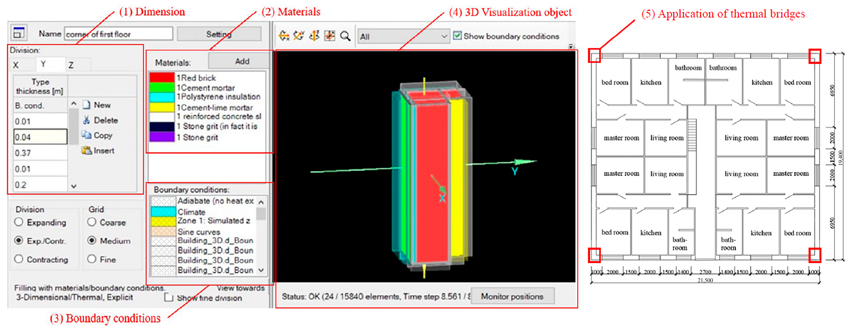
Another approach examines the influence of thermal bridges on the energy performance of Chinese residential buildings through a detailed 3D Dynamic Modeling Method [79]. It uses WUFI Plus 3.3 software to simulate thermal bridges in three dimensions, accounting for exact geometries, material properties and boundary conditions (Figure 10). The results show that ignoring thermal bridges leads to a significant underestimation of energy demand (about 21.2% to 27.8% for annual heating, depending on the climate zone), and the simplified method consistently underestimates both heating and cooling demands compared to the dynamic approach, which accurately includes thermal inertia and avoids double-counting of wall volumes.

Another remarkable and easy-to-implement method is the U-value modified (U_mod) [80], which adjusts the insulation level of a 1D multi-layer envelope so that its thermal transmittance reflects the overall U-value, including thermal bridge effects. The following formula is used for the calculation of the U_mod from the homogeneous wall’s thermal transmittance to consider the linear and point thermal transmittance.

$${\mathrm{U}}_{\mathrm{mod}}={\displaystyle \frac{\mathrm{U}·\mathrm{A}+{{\displaystyle \sum }}_{\mathrm{j}=1}^{\mathrm{n}}({\mathsf{\psi }}_{\mathrm{j}}·{\mathrm{L}}_{\mathrm{j}})+{\sum }_{\mathrm{k}=1}^{\mathrm{p}}({\mathsf{\chi }}_{\mathrm{k}})}{\mathrm{A}}}$$

(2)

where

• U_mod is the modified homogeneous wall thermal transmittance (W/m²K);
• U is the thermal transmittance of the component and envelope without the impact of linear or point thermal bridges taken into consideration (W/m²K);
• A is the area over which the U_mod values apply (m²);
• Ψ_j is the linear thermal transmittance of the j_-th linear thermal bridge (W/mK);
• L_j is the length of the j-th linear thermal bridge (m);
• Χ_k is the point thermal transmittance of the k_-th point thermal bridge (W/K).

In this process, usually the conductivity of one layer is modified (often the insulation) to adjust the starting U-value, while the other material properties of the multi-layered components remain unchanged. In such regard, the following equation, adapted from [61], can be used to calculate the equivalent thermal conductivity (λ_equi) to be applied to the multi-layered envelope component that takes into account the thermal bridges:

$${\mathsf{\lambda }}_{\mathrm{equi}}={\displaystyle \frac{1}{\left(\frac{1}{{\mathsf{\lambda }}_{\mathrm{i}}}-\frac{\mathrm{R}-{\mathrm{R}}_{\mathrm{mod}}}{{\mathrm{d}}_{\mathrm{i}}}\right)}}$$

(3)

where

• λ_equi is the equivalent thermal conductivity of the layer of a multi-layered envelope component to be modified (W/mK);
• λ_i is the original thermal conductivity of the layer selected (W/mK);
• R is the thermal resistance of the component without the effects of the thermal bridges, calculated as the inverse of U (m²K/W);
• R_mod is the thermal resistance of the component with the effects of the thermal bridges, calculated as the inverse of U_mod (m²K/W);
• d_i is the thickness of the layer on which λ_i value is changed (m).

It should be noted that this approach ignores the variation of the thermal capacity caused by the thermal bridges, which also alters the dynamic characteristics of opaque walls [81]. In such respect, another method, known as the Combined Thermal Properties (CTP) [82], introduced a refined approach by adjusting density and specific heat to reflect actual thermal capacity. Typically, CTP uses a single modified layer, but it can be adapted within U_mod to estimate adjusted values in multi-layer components. In this sense, the following formula can be used to calculate the adjusted density. Analogue calculations can be done for the specific heat parameter.

$${\mathsf{\rho }}_{\mathrm{s}}={{\displaystyle \sum }}_{\mathrm{i}=1}^{\mathrm{n}}{\mathrm{C}}_{\mathrm{i}}·{\mathsf{\rho }}_{\mathrm{i}}$$

(4)

where

• ρ_s is the adjusted density of the whole component (kg/m³);
• C_i is the volumetric fraction of the material i;
• ρ_i is the density of the material i (kg/m³).

C_i is calculated by the ratio of the volume of a single material layer (V_i) and the volume of the whole component (V_s). Based on this, some authors applied the CTP method to implement the dynamic effect of steel framing in the EnergyPlus program, which led to an increase of the peak thermal load and annual energy consumption of approximately 10% and 5%, respectively [82]. However, this formula assumes that the thermal mass of the component can be represented through a homogenized volumetric averaging approach, where the contribution of each material layer is proportional to its volume fraction. As a result, local thermal heterogeneities, material discontinuities, and complex transient heat transfer effects are not explicitly represented.

It should be noted that the U_mod method requires the linear and point thermal transmittance, which are usually calculated through separate software. For example, Jan et al. [83] use THERM, which is a two-dimensional conduction heat-transfer analysis program developed by Lawrence Berkeley National Laboratory, to calculate the effective linear thermal transmittance of thermal bridges under steady-state conditions. Such a tool supports simplified geometry inputs and can be combined with BES to capture dynamic effects.

Some authors [84,85] compared U_mod and the equivalent wall method and found that while both underestimated cooling loads in hot climates, the equivalent wall method performed better. The peak load was underestimated by 8–13% when using the U_mod method and by 4–9% with the equivalent wall method. Additionally, the annual cooling load was underestimated by 17% and 14%, respectively. Despite better accuracy, the complexity of generating equivalent wall properties limits its practical use. Minimizing thermal bridges can reduce simulation errors [86].

Baba et al. [87] and Kotti et al. [88] show that the U_mod method based on 2D thermal bridge modeling could slightly underestimate heating loads compared to 3D modeling, particularly in buildings with large balconies and high insulation. Thermal breaks at junctions improve accuracy by reducing heat loss. Similarly, Chen et al. [79] stress the need for 3D dynamic simulations to ensure reliable energy performance assessments. As highlighted by some authors [89], the 3D thermal bridge simulation provides surface temperatures up to 6 K lower than 2D models under the same conditions. Such a difference needs to be considered since it increases the risk of condensation and mold.

With increasingly complex envelopes, moving beyond steady-state methods is essential. Dynamic modeling better captures daily fluctuations and solar gains. In BES, thermal bridges are typically integrated by adjusting the building component, surfaces or the definition of specific transmission coefficients of building elements. This is usually based on the calculation of linear/point thermal transmittance through 2D models with FEM simulations, or a more accurate approach through 3D modeling [79].

It should be noted that although numerous abacus and databases provide common constructive joints for different thermal bridges and the related linear thermal transmittance, they may introduce errors of up to 35% in historic buildings due to a lack of detail on traditional materials and joints [67]. Accurate modeling is therefore critical for retrofit planning, heat loss reduction, and moisture control, particularly in heritage contexts.

3.4.2. Punctual Thermal Bridges

Although most studies address linear thermal bridges, the impact of punctual thermal bridges is often neglected, as their contribution is typically minor and localized in standard envelopes [90]. While this leads to negligible error, some authors call for improved accuracy [69,91]. In addition, it is difficult to evaluate the point thermal transmittance without special software due to its calculation complexity [80].

The following formula is used for the calculation of the direct heat transfer coefficient, including the contribution due to all thermal bridges, according to EN ISO 14683 [63]:

$$\mathsf{\chi }={\mathrm{L}}_{3\mathrm{D}}-{{\displaystyle \sum }}_{\mathrm{i}=1}^{{\mathrm{N}}_{\mathrm{i}}}{\mathrm{U}}_{\mathrm{i}}·{\mathrm{A}}_{\mathrm{i}}-{{\displaystyle \sum }}_{\mathrm{j}=1}^{{\mathrm{N}}_{\mathrm{j}}}{\mathsf{\psi }}_{\mathrm{j}}·{\mathrm{L}}_{\mathrm{j}}$$

(5)

where

• Χ is the point thermal transmittance of the thermal bridges;
• L_3D is the thermal coupling coefficient obtained from a 3-D calculation of the 3-D component separating the two environments being considered (W/K);
• U_i is the thermal transmittance of the 1-D component i separating the two environments being considered (W/m²K);
• A_i is the area over which the value U_i applies;
• Ψ_j is the linear thermal transmittance of the j_-th linear thermal bridge (W/mK);
• L_j is the length of the j_-th linear thermal bridge (m).

It should be noted that punctual thermal bridges, like linear thermal bridges, can be implemented in BES with the same procedures described in the previous section.

Although there are few analyses of point thermal bridges in historic buildings in the literature, it is considered useful to report a brief examination of their impact in some more recent case studies. In such respect, Jolanta et al. [90,92] analyzed aluminum fasteners in façade cladding and found they can increase the overall wall U-value by up to 30%, depending on the material properties and dimensions of external layers. As the thickness of the bearing layer and the thermal conductivity value of the insulation layer increased, the punctual thermal transmittance decreased by up to 28%. Additionally, a simplified methodology was presented to assess punctual thermal bridges using empirical relationships based on the thermal and geometric properties of the external wall layers. Theodosiou et al. [93] performed a parametric study on lightweight cladding systems, showing that punctual thermal bridges can account for 5–20% of total heat flow, influenced by wall transmittance and cavity ventilation, with effects comparable to linear thermal bridges.

During an investigation of the anchors in the ETICS system, Orlik–Kożdoń et al. [94] applied the program THERM 7.4 for the thermal modeling of the punctual thermal bridge with only the features of the connector and sleeves, and base material conductivities. They observed high compliance between modeling results and measurements. In measurements with a significant temperature difference (ΔT = 40 °C), the discrepancy in temperature values compared to the modeling was only 0.1 to 0.2 °C, within acceptable error margins.

Martin et al. [61,68] also applied their equivalent wall method with three homogeneous layers to the pillar thermal bridge, blind box and lintel thermal bridge. Under dynamic outdoor conditions, low thermal capacity bridges (e.g., blind box, lintel) showed higher residuals: 0.5 K (inner surface temperature), 1.4 K (outer surface temperature), 4.06 W/m² (heat flow). In contrast, pillar thermal bridges with similar inertia to the homogeneous wall had much lower residuals: 0.1 K, 0.6 K, and 0.45 W/m², closely matching 3D modeling results. Viot et al. [60] extended the method to wood-frame construction and found it suitable for high-inertia elements like concrete, but less accurate for lightweight assemblies, where amplitude and phase shift were poorly captured. The findings suggest that steady-state values from catalogues are often insufficient, and even dynamic studies may not yield universally reliable simplifications.

4. Discussion and Recommendations

As outlined in the previous sections, the geometric representation and simplification of real structures for building energy modeling involves numerous factors that must be carefully addressed. A review of the literature, with specific reference to historic buildings, has revealed that several critical aspects must be considered when dealing with this specific building typology.

Given the growing role of energy simulation in assessing building efficiency and certification, adopting accurate and reliable modeling practices is essential. This is especially true in the case of historic buildings, where challenges related to data availability and geometric complexity are significantly more pronounced. In this regard, for each issue addressed in the previous section, the identification of the proper procedures will be proposed with specific reference to historic buildings (

Table 2. Summary of geometric simplification methods with advantages and limitations by topic.

Topic	Method	Advantages	Limitations	Refs.
Thermal zones–Grouping of thermal zones	Zoned by floor	Simple and fast to model	Limited accuracy, particularly in buildings with irregular layouts or varying usage	[14,15]
	Core and perimeter			[17]
	Koopman operator	High accuracy	A detailed model of all the zones must first be created, time-consuming	[20,21,22]
	Zoned by orientation	Captures solar gains and external heat exchange more accurately	May neglect functional and occupancy variations within the same orientation	[18,19]
	Zoned by schedule	Improves simulation of internal load variation and HVAC control	Requires detailed usage data and may overlook thermal envelope influences	[23]
	Zoned by air conditioning	Reflects system performance and control more realistically	Does not account for passive gains or orientation-specific effects	[24]
	Zoned based on standards by function, orientation and schedule	Balance between accuracy and modeling efficiency; adaptable to diverse building types and usage patterns	May require more initial data collection and model setup	[16,25,26]
Thermal zones–Inside, center or outside perimeter	Outside dimensions for all surfaces	Accurate on outdoor solar radiation and heat gains	Overestimates the volume	[19,25]
	Inside dimensions for all surfaces	Accurate on building area and interior room volume	Inaccuracy in thermal mass and envelope area estimation	[19,25]
	Centerline dimensions for all surfaces	Balance between the above two methods	Better consider the thermal mass of buildings with huge thick walls	[19,25,30]
	Outside dimensions for exterior surfaces and centerline dimensions for the interior surfaces	Balance between heat gain and volume	Inaccuracy in buildings with very thick walls	[28,29,30]
Thermal zones–Construction of part or all of the building	Three Representative Floors	Significant reduction in modeling and simulation time, widely supported in tools like EnergyPlus	Loss of vertical variability, cannot fully reflect complex airflow or radiation dynamics in connected spaces like staircases	[19,24,31,32]
	Five or More Representative Floors (e.g., 5, 7, 9 Floors)	Improved accuracy in capturing thermal gradients and energy demands across height	Performance details of non-simulated floors are inferred, not explicitly modeled	[24,32]
	Co-simulation of Simpler Sub-Buildings	Allows parallel computation, scalable to complex or modular buildings	Requires robust and well-defined boundary conditions, which can be hard to establish in practice	[33]
Thermal zones–Irregular shapes	Zone squaring	Significantly reduces input complexity and modeling time	Oversimplifies spatial heterogeneity, potentially misrepresenting internal heat gains, airflows, and exposure	[31,34]
	Reduce sides of planar for curved surfaces	Maintains the overall massing and orientation	Risk of thermal and solar gain misrepresentation	[3]
	Reduce low polygon mesh for curved surfaces	Maintains topological continuity better than planar segmentation	Risk of thermal and solar gain misrepresentation	[36]
Opaque surfaces–Not homogeneous stratigraphies	1D series model	Easy to implement, fast computation, better accuracy if material properties and proportions are known	Underestimates heat/moisture transfer, cannot capture lateral effects, inaccurate with voids	[43,44,46,47]
	1D blended model (Homogeneous wall model)	Simple geometry, useful when material differences are small	Oversimplifies composition and geometric complexity, inaccurate vapor resistance, not sensitive to voids	[40,43,44]
	1D blended external + core model	Better than fully blended models, performs well in drying/wetting simulations	Ignores detailed geometric irregularity, affects thermal inertia and hygrothermal performance	[44,47]
	2D parallel model	Higher accuracy for thermal/moisture flow, captures mortar joints explicitly	Moderate modeling and computing effort, accuracy depends on void assumptions	[44,45]
Opaque surfaces–Surface irregularities	Exclusion of shading elements	Reduces modeling complexity, effective when low solar exposure	Overestimation of solar gains for south-facing facades with significant glazing, skew seasonal heat balance	[23]
Transparent surfaces–Surfaces grouping	Surfaces grouping	Reduces modeling complexity, useful for early-stage design or large-scale modeling	Frame effects are ignored, reduces accuracy in thermal losses and solar performance analysis	[25,27,31]
Transparent surfaces–Window frames, glazing area partitioning and window position	Accurate window geometry but without frame or border shading	Reduces modeling complexity, retains geometric realism	Not suitable for shading-critical analyses, less accurate in thermal bridging and passive design studies	[27,54]
	Constant U-value, SHGC, and transmittance	Fast computation and low data requirements, can be corrected with a factor	Ignores temperature and angle dependency of glazing	[55,56]
	Rectangular approximation of complex windows	Retains optical and thermal area characteristics; simpler modeling	May miss solar gain nuances caused by curvature and shading angles	[53,57]
	Detailed window modeling via specialized software	Highly detailed, captures frame effects and thermal bridges, reliable solar/shading data	Requires extensive input data, time-consuming, demands advanced user knowledge	[58]
	Three-step window transmittance calculation approach	Allows partial modeling when full data is missing, aligns with standards	Requires simulation tools for frame/spacer modeling, more complex than standard simplification	[59]
Thermal bridges–Existing methods for the evaluation of thermal bridges in energy simulation	Abacus/catalogues	Easy to implement, it does not require any separate calculations but is based on data that is already available	Fail to capture the transient thermal behavior and the role of thermal inertia within the envelope. Limited to common and typical architectural configurations, while if applied to non-standard constructions, it can lead to high discrepancies	[65,66,67]
	U-value modified method	Simple, easy integration, minimal input, allows simulation of localized 2D effects	Ignores the variation of the thermal capacity, but can be captured by CTP method	[4,79,82,83,87,88]
	Equivalent wall method	Good accuracy in representing both steady-state and transient behavior	Computational setup is more complex than basic methods	[61,68,69,70,71,72,73,74,75,76,77,78,84,85,86]
	3D Dynamic Modelling Method	High accuracy in both steady-state and dynamic conditions, captures complex 3D heat flow and material interfaces	Time-consuming, requires detailed geometric and material input, not directly supported in most BES tools	[79,87,88,89]
Thermal bridges–Punctual thermal bridges	U-value modified method	Simple, easy integration, minimal input, accurate for connector-related thermal bridges	Mainly steady-state analysis, Simplified assumptions may not capture full dynamic behavior	[94]
	Equivalent wall method	Good agreement with 3D models for high-inertia components	Poor accuracy for low-inertia or lightweight assemblies, Difficulty capturing amplitude and phase shift under dynamic conditions	[60,61,68]
	3D Dynamic Modelling Method	High accuracy in both steady-state and dynamic conditions, captures complex 3D heat flow and material interfaces	Time-consuming, requires detailed geometric and material input, not directly supported in most BES tools	[60,61,68,94]

).

Concerning the definition of thermal zones, as extensively discussed, the aggregation of thermal zones is a permitted and commonly adopted practice. The analyzed studies show that the thermal zone grouping can significantly reduce simulation time, while oversimplification may lead to substantial differences (in a range of about 3–26%) in building energy simulation results. The variation in the reported error ranges across studies can be attributed to several factors, including differences in climate conditions, building typologies, occupancy patterns, simulation tools, and the degree of simplification applied during the thermal zoning process. In particular, buildings with highly heterogeneous spatial functions or varying solar exposure tend to be more sensitive to zone aggregation strategies, which leads to larger deviations in simulation outcomes. These studies provided a consensus regarding the criteria for dividing thermal zones, including solar gain, orientation, occupancy, schedule and space function. These factors clearly illustrate the concept of thermal zoning. However, existing literature has not provided a comprehensive set of rules for thermal zoning; instead, it has only offered general guidelines and considerations for engineers when designing a building’s thermal zones. As a result, many designs tend to rely on the engineer’s experience and intuition for thermal zoning. Therefore, a standardized thermal zoning method should be developed and considered as a future research direction.

Regarding the reference line used to define the volume of thermal zones, as previously discussed, the choice between the external, central, or internal perimeter can introduce simulation errors ranging from approximately 2% to as much as 14%, while for historic buildings, due to their thick walls, the definition of the boundaries will have greater impacts, and proper application should be more carefully addressed. Some studies suggest considering outside dimensions for exterior surfaces and centerline dimensions for the interior surfaces to properly calculate the floor area, zone volume and thermal mass. Moreover, it is recommended for buildings with huge thick walls to use the centerline dimensions for all surfaces (exterior and interior) to properly consider the given thermal mass, avoiding the overestimation of the volume. Regarding the buildings with repeated floor layouts, it can be simplified by simulating a single representative intermediate floor, in addition to the ground and top floors. Energy demand and peak load estimates are calculated by multiplying the results for the representative floor by the number of similar levels and then adding the values for the ground and top floors. Some studies also add the results of some other intermediate floors to limit the simulation error below 10%.

In historic building energy models, the occurrence and simplification of irregular shapes are often unavoidable, and inaccuracies resulting from oversimplification in some geometrical characteristics must be avoided. Some common methods for modeling thermal zones of irregular shapes are polygonising the shape, like flattening the boundaries, and producing a low-polygon mesh of the original surfaces, in which the relationship between simulation run time and geometric complexity needs to be balanced. Opaque surfaces play a pivotal role in building energy simulations, particularly in historic structures with complex geometries and heterogeneous materials. Although geometric simplifications and average thickness are commonly applied, non-homogeneous stratigraphies introduce significant uncertainties in thermal modeling. Studies reveal that calculated U-values often overestimate real performance due to material variability and composition. Advanced modeling approaches, such as detailed 2D representations or blended material methods, improve accuracy but require more effort. Simplified models must carefully consider material proportions (e.g., stone, mortar, voids) to reflect actual conditions. Therefore, reliable simulations require calibrated parameters and detailed construction knowledge to avoid errors, especially when planning retrofit interventions.

Regarding transparent surfaces, historic windows often feature irregular shapes, posing challenges for energy modeling due to missing material properties and the need for geometric simplifications. Thick walls typical of historic buildings can influence window performance by reducing solar gains, an effect sometimes significant depending on orientation, location, and wall thickness. Simplifications often exclude frames, assuming fully glazed surfaces. Studies show this approach in some very simple cases introduces negligible errors, however, in cold climates, detailed modeling reveals greater heat losses and lower cooling needs compared to simplified models, with energy demand differences up to 7–23%. Simplifying complex window geometries by preserving total opening areas ensures accurate solar and ventilation modeling. For more precise simulations, tools such as WINDOW 5 can model frame and glazing interactions, accounting for thermal bridges and shading effects, though requiring more detailed data and expertise.

The implementation of thermal bridges is essential in historic buildings due to their impact on dynamic thermal behavior. In BES, they are often integrated by adjusting building components, surfaces or assigning specific transmission coefficients. This is typically achieved by calculating linear or point transmittance values using 2D FEM simulations or more advanced 3D modeling.

Some studies have introduced the equivalent wall method to model thermal bridges dynamically by replacing a complex junction with a 1D multi-layer structure that replicates its thermal behavior, and a three-layer wall is usually sufficient. Another simple and widely used method in the literature is the U_mod method. The method adjusts insulation to match the overall U-value of the structure, including thermal bridges without changing material properties. The CTP method refines this by also modifying density and specific heat to better represent thermal capacity. Tools like THERM can directly calculate the effective linear thermal transmittance of thermal bridges under steady-state conditions, which can then be imported into the energy simulation software as inputs.

Comparing the two methods, the equivalent wall method performs slightly better but still underestimates the heating and overestimates the cooling energy demand with an average error ranging from 4 to 14%. However, considering the complexity of generating the thermal properties of equivalent wall layers required, it seems unsuitable for practical use.

On the contrary, the 3D dynamic modeling method may still be required for buildings with high insulation and thermal mass but with poor connection details, and improving the connection details and minimizing thermal bridges can reduce the error in the simplified method. Furthermore, the analysis of punctual thermal bridges is more complex. While often negligible in conventional envelopes, they can cause significant estimation errors in systems using metal connectors, such as cladding supports. Punctual thermal bridges can be implemented in BES using methods similar to those for linear thermal bridges. The analyzed studies show that the influence of punctual thermal bridges ranges from 5 to 30% on the envelope’s thermal performance. Some studies use 3D FEM simulations to evaluate punctual bridges and propose empirical methods, which give a sufficiently precise (95%) result. Other studies tried to apply the simplified model with the U_mod and the equivalent wall method, but these are only reliable when the thermal inertia is close to that of the homogeneous wall. For low-inertia bridges, average surface temperature errors can be five times higher (0.2–1 °C). Therefore, no simplified model fits all cases, and 3D dynamic modeling remains the most reliable solution for capturing their thermal behavior. Such a model could be integrated using commercial simulation tools, which allow the integration of reduced models [95].

5. Conclusions

Buildings consume a significant amount of energy due to their continuous operation and long lifetime. Conducting building energy simulations is a crucial aspect of the decision-making process, as it helps designers to assess the energy and comfort effects of different building design options. The geometric simplifications in modeling can save a significant amount of time on simulations, while oversimplification may lead to significant differences in building energy simulation results and needs to be balanced, especially for the geometric simplification of historic buildings, which plays a crucial role in facilitating accurate, efficient, and feasible energy modeling processes. Due to the intricate and often irregular nature of heritage structures, direct modeling of their full geometric complexity can lead to excessive computational demands and impractical simulation workflows. Geometric simplification thus enables the preservation of critical thermal and morphological characteristics while significantly reducing model complexity, making energy analysis more accessible for conservation, retrofitting, and policy-making purposes. In summary, the geometric simplification of historic buildings constitutes a fundamental process in the development of accurate and computationally efficient energy models.

However, the impacts of building physics simulation model simplifications on the accuracy of the results are not well studied and reported. The balance between model accuracy and computational efficiency during the geometric simplification process remains an area that has not been thoroughly investigated. Existing studies often prioritize one aspect at the expense of the other, leading to either oversimplified models that compromise thermal performance predictions or overly detailed models that are computationally prohibitive. Some studies only offer general guidelines and considerations, while still relying on the engineer’s experience and intuition. A systematic exploration of optimization strategies that simultaneously consider accuracy and efficiency is still lacking, especially in the context of the unique challenges posed by historic buildings. Therefore, it is usually necessary to study how to simplify the energy model of historic buildings in the geometric modeling stage.

Under these premises, the present work has systematically reviewed four key components of this process: the definition of thermal zones, the simplification of opaque and transparent surfaces, and the implementation of thermal bridges. Each component poses distinct challenges, particularly given the architectural complexity and historic value of heritage buildings. Nonetheless, judicious simplification strategies that maintain the essential thermal and spatial characteristics can significantly enhance the reliability of simulation outcomes while reducing computational demands. Based on the review, the work tries to highlight the main issues and make recommendations for each component in the modeling process. The review also reveals that different geometric simplification strategies may lead to substantially different impacts on simulation accuracy depending on the building component and modeling approach adopted. In particular, the use of standardized thermal bridge catalogues in historic buildings may introduce errors of up to 35%, highlighting the limitations of applying generalized assumptions to historic structures characterized by irregular geometries and heterogeneous construction systems. This finding underlines the importance of carefully balancing modeling simplification and physical accuracy, especially in retrofit-oriented simulations where reliable thermal assessments are essential.

In conclusion, the information collected in this work can provide a set of geometric modeling methodologies for the energy simulation of historic buildings at the geometric modeling stage, which will be useful for modelers to determine the optimal level of model simplification in their project and offer a significant contribution to the development of new rules and strategies. The analysis efficiency of energy retrofit of historic buildings will also be further improved, especially for projects that require a lot of simulation. Moreover, having more accurate simulation models is increasingly important in the current context of climate policy and energy regulation. They support more reliable energy certification, contribute to meeting greenhouse gas reduction targets, and allow for a better estimation of energy consumption, particularly in the retrofit of historic buildings. Overall, the work reinforces the role of simulation as a critical tool in aligning heritage conservation with sustainability goals.

References

1. European Commission—Department Energy. In Focus: Energy Efficiency in Buildings; European Commission: Brussels, Belgium, 2020. [Google Scholar]
2. Mazzeo, D.; Matera, N.; Cornaro, C.; Oliveti, G.; Romagnoni, P.; De Santoli, L. EnergyPlus, IDA ICE and TRNSYS Predictive Simulation Accuracy for Building Thermal Behaviour Evaluation by Using an Experimental Campaign in Solar Test Boxes with and without a PCM Module. Energy Build. 2020, 212, 109812. [Google Scholar] [CrossRef] [Scilit]
3. Chatzivasileiadi, A. Addressing Pathways to Energy Modelling Through Non-Manifold Topology. In Proceedings of the 2018 Symposium on Simulation for Architecture and Urban Design (SimAUD 2018); Society for Modeling and Simulation International (SCS): Delft, The Netherlands, 2018. [Google Scholar]
4. Akkurt, G.G.; Aste, N.; Borderon, J.; Buda, A.; Calzolari, M.; Chung, D.; Costanzo, V.; Del Pero, C.; Evola, G.; Huerto-Cardenas, H.E.; et al. Dynamic Thermal and Hygrometric Simulation of Historical Buildings: Critical Factors and Possible Solutions. Renew. Sustain. Energy Rev. 2020, 118, 109509. [Google Scholar] [CrossRef] [Scilit]
5. Webb, A.L. Energy Retrofits in Historic and Traditional Buildings: A Review of Problems and Methods. Renew. Sustain. Energy Rev. 2017, 77, 748–759. [Google Scholar] [CrossRef] [Scilit]
6. Macdonald, I.A. Quantifying the Effects of Uncertainty in Building Simulation. Doctoral Dissertation, University of Strathclyde, Glasgow, UK, 2002. [Google Scholar]
7. Negendahl, K. Building Performance Simulation in the Early Design Stage: An Introduction to Integrated Dynamic Models. Autom. Constr. 2015, 54, 39–53. [Google Scholar] [CrossRef] [Scilit]
8. Tronchin, L.; Fabbri, K. Energy and Microclimate Simulation in a Heritage Building: Further Studies on the Malatestiana Library. Energies 2017, 10, 1621. [Google Scholar] [CrossRef] [Scilit]
9. Building Research Establishment. BRE National Calculation Methodology Modelling Guide; BRE: Watford, UK, 2021. [Google Scholar]
10. Natural Resources Canada’s Office. Canadian Standardization Method EE4; Natural Resources Canada: Ottawa, ON, Canada, 2008.
11. ANSI/ASHRAE/IES Standard 90.1-2022; Energy Standard For Buildings. ASHRAE: Atlanta, GA, USA, 2022.
12. Commercial Energy Services Network. Commercial Buildings Energy Modeling Guidelines and Procedures; Commercial Energy Services Network: Washington, USA, 2010. [Google Scholar]
13. Shin, M.; Haberl, J.S. Thermal Zoning for Building HVAC Design and Energy Simulation: A Literature Review. Energy Build. 2019, 203, 109429. [Google Scholar] [CrossRef] [Scilit]
14. Korolija, I.; Zhang, Y. Impact of Model Simplification on Energy and Comfort Analysis for Dwellings. In Proceedings of the 2017 Building Simulation Conference; IBPSA: Savoie, France, 2013. [Google Scholar]
15. Picco, M.; Marengo, M. On the Impact of Simplificationson Building Energy Simulation for Early Stage Building Design. J. Eng. Archit. 2015, 3, 66–78. [Google Scholar] [CrossRef] [Scilit]
16. Heo, Y.; Ren, G.; Sunikka-Blank, M. Investigating an Adequate Level of Modelling for Energy Analysis of Domestic Buildings. In Proceedings of the Asim 2016; IBPSA: Jeju, Republic of Korea, 2016. [Google Scholar]
17. Dogan, T.; Saratsis, E.; Reinhart, C. The Optimization Potential of Floorplan Typologies in Early Design Energy Modeling. In Proceedings of the 2015 Building Simulation Conference; IBPSA: Hyderabad, India, 2015. [Google Scholar]
18. O’Brien, W.; Athienitis, A.; Kesik, T. Thermal Zoning and Interzonal Airflow in the Design and Simulation of Solar Houses: A Sensitivity Analysis. J. Build. Perform. Simul. 2011, 4, 239–256. [Google Scholar] [CrossRef] [Scilit]
19. Dipasquale, C.; D’Antoni, M.; Fedrizzi, R. The Effect of the Modelling Approach on the Building’s Loads Assessment. In Proceedings of the Energy Forum on Advanced Building Skins; Energy-Forum GmbH: Bressanone, Italy, 2013. [Google Scholar]
20. Georgescu, M.; Eisenhower, B.; Mezić, I. Creating Zoning Approximations to Building Energy Models Using the Koopman Operator. In Proceedings of the SimBuild Conference 2012; IBPSA: Madison, WI, USA, 2012; Volume 5, pp. 40–47. [Google Scholar]
21. Georgescu, M.; Mezić, I. Building Energy Modeling: A Systematic Approach to Zoning and Model Reduction Using Koopman Mode Analysis. Energy Build. 2015, 86, 794–802. [Google Scholar] [CrossRef] [Scilit]
22. Giannakis, G.I.; Kontes, G.D.; Korolija, I.; Rovas, D.V. Simulation-Time Reduction Techniques for a Retrofit Planning Tool. In Proceedings of the 2017 Building Simulation Conference; IBPSA: San Francisco, CA, USA, 2017; Volume 15, pp. 2014–2023. [Google Scholar]
23. Klimczak, M.; Bojarski, J.; Ziembicki, P.; Kȩskiewicz, P. Analysis of the Impact of Simulation Model Simplifications on the Quality of Low-Energy Buildings Simulation Results. Energy Build. 2018, 169, 141–147. [Google Scholar] [CrossRef] [Scilit]
24. Jung, Y.; Heo, Y.; Lee, H. Multi-Objective Optimization of the Multi-Story Residential Building with Passive Design Strategy in South Korea. Build. Environ. 2021, 203, 108061. [Google Scholar] [CrossRef] [Scilit]
25. Zhao, J.; Wu, Y.; Shi, X.; Jin, X.; Zhou, X. Impact of Model Simplification at Geometric Modelling Stage on Energy for Office Building. In Proceedings of the BSO Conference 2018; IBPSA-England: Cambridge, UK, 2018; Volume 4, pp. 402–406. [Google Scholar]
26. Elhadad, S.; Radha, C.H.; Kistelegdi, I.; Baranyai, B.; Gyergyák, J. Model Simplification on Energy and Comfort Simulation Analysis for Residential Building Design in Hot and Arid Climate. Energies 2020, 13, 1876. [Google Scholar] [CrossRef] [Scilit]
27. Bishop, D.; Mohkam, M.; Williams, B.L.M.; Wu, W.; Bellamy, L. The Impact of Building Level of Detail Modelling Strategies: Insights into Building and Urban Energy Modelling. Eng 2024, 5, 2280–2299. [Google Scholar] [CrossRef] [Scilit]
28. Ladenhauf, D.; Battisti, K.; Berndt, R.; Eggeling, E.; Fellner, D.W.; Gratzl-Michlmair, M.; Ullrich, T. Computational Geometry in the Context of Building Information Modeling. Energy Build. 2016, 115, 78–84. [Google Scholar] [CrossRef] [Scilit]
29. Ladenhauf, D.; Berndt, R.; Krispel, U.; Eggeling, E.; Ullrich, T.; Battisti, K.; Gratzl-Michlmair, M. Geometry Simplification According to Semantic Constraints: Enabling Energy Analysis Based on Building Information Models. Comput. Sci.-Res. Dev. 2016, 31, 119–125. [Google Scholar] [CrossRef] [Scilit]
30. U.S. Department of Energy. Tips and Tricks for Using EnergyPlus; U.S. Department of Energy: Washington, DC, USA, 2022.
31. Picco, M.; Lollini, R.; Marengo, M. Towards Energy Performance Evaluation in Early Stage Building Design: A Simplification Methodology for Commercial Building Models. Energy Build. 2014, 76, 497–505. [Google Scholar] [CrossRef] [Scilit]
32. Ellis, P.G.; Torcellini, P.A. Simulating Tall Buildings Using Energyplus. In Proceedings of the Building Simulation 2005; IBPSA: Montreal, QC, Canada, 2005; Volume 9, pp. 279–286. [Google Scholar]
33. Giannakis, G.; Pichler, M.; Kontes, G.; Schranzhofer, H.; Rovas, D. Simulation Speedup Techniques for Computationally Demanding Tasks. In Proceedings of the 2017 Building Simulation Conference; IBPSA: Chambery, France, 2013. [Google Scholar]
34. Beltrami, A.; Picco, M.; Marengo, M. Comparison of Energy Simulations for a Residential Unit: A Rapid Method for an Integrated Decision Tool. In Proceedings of the BSA Conference 2015; IBPSA-Italy: Bozen-Bolzano, Italy, 2015; Volume 2, pp. 137–145. [Google Scholar]
35. Chatzivasileiadi, A.; Hosney Lila, A.M.; Lannon, S.; Jabi, W. The Effect of Reducing Geometry Complexity on Energy Simulation Results. In Proceedings of the eCAADe 2018: Computing for a Better Tomorrow; eCAADe: Łódź, Poland, 2018; pp. 559–568. [Google Scholar]
36. Santos, L.; Schleicher, S.; Caldas, L. Automatic Simplification of Complex Building Geometry for Whole-Building Energy Simulations. In Proceedings of the Building Simulation 2019; IBPSA: Rome, Italy, 2019; pp. 2691–2698. [Google Scholar]
37. Coelho, G.B.A.; Silva, H.E.; Henriques, F.M.A. Calibrated Hygrothermal Simulation Models for Historical Buildings. Build. Environ. 2018, 142, 439–450. [Google Scholar] [CrossRef] [Scilit]
38. Ascione, F.; Ceroni, F.; De Masi, R.F.; de’ Rossi, F.; Pecce, M.R. Historical Buildings: Multidisciplinary Approach to Structural/Energy Diagnosis and Performance Assessment. Appl. Energy 2017, 185, 1517–1528. [Google Scholar] [CrossRef] [Scilit]
39. Maldague, X. Theory and Practice of Infrared Technology for Nondestructive Testing; A Wiley-Interscience publication; John Wiley & Sons: Hoboken, NJ, USA, 2001. [Google Scholar]
40. Roberti, F.; Oberegger, U.F.; Gasparella, A. Calibrating Historic Building Energy Models to Hourly Indoor Air and Surface Temperatures: Methodology and Case Study. Energy Build. 2015, 108, 236–243. [Google Scholar] [CrossRef] [Scilit]
41. Litti, G.; Khoshdel, S.; Audenaert, A.; Braet, J. Hygrothermal Performance Evaluation of Traditional Brick Masonry in Historic Buildings. Energy Build. 2015, 105, 393–411. [Google Scholar] [CrossRef] [Scilit]
42. Rye, C.; Scott, C. The Spab U-Value Report; Society for the Protection of Ancient Buildings: London, UK, 2012. [Google Scholar]
43. Paul, B. Historic Scotland Techpaper 10; Historic Scotland: Edinburgh, UK, 2011.
44. Gutland, M.; Bucking, S.; Santana Quintero, M. Hygrothermal Modelling of Historic Rubble Masonry Walls: Accounting for Geometric and Compositional Variability. J. Build. Eng. 2022, 48, 103929. [Google Scholar] [CrossRef] [Scilit]
45. Pascucci, M.; Lucchi, E. 2D-Hygrothermal Simulation of Historical Solid Walls. In Proceedings of the CAADence in Architecture, Back to Command; Budapest University of Technology and Economics: Bolzano, Italy, 2016; pp. 155–161. [Google Scholar]
46. Lucchi, E. Thermal Transmittance of Historical Stone Masonries: A Comparison among Standard, Calculated and Measured Data. Energy Build. 2017, 151, 393–405. [Google Scholar] [CrossRef] [Scilit]
47. Little, J.; Ferraro, C.; Arregi, B. Assessing Risks in Insulation Retrofits Using Hygrothermal Software Tools; Technical Paper 15; Historic Environment Scotland: Scotland, UK, 2015. [CrossRef]
48. Genova, E.; Fatta, G. The Thermal Performances of Historic Masonry: In-Situ Measurements of Thermal Conductance on Calcarenite Stone Walls in Palermo. Energy Build. 2018, 168, 363–373. [Google Scholar] [CrossRef] [Scilit]
49. Cascardi, A.; Longo, F.; Perrone, D.; Lassandro, P.; Aiello, M.A. Thermography Investigation and Seismic Vulnerability Assessment of a Historical Vaulted Masonry Building. Heritage 2022, 5, 2041–2061. [Google Scholar] [CrossRef] [Scilit]
50. Lucchi, E. Applications of the Infrared Thermography in the Energy Audit of Buildings: A Review. Renew. Sustain. Energy Rev. 2018, 82, 3077–3090. [Google Scholar] [CrossRef] [Scilit]
51. Giuliani, M.; Henze, G.P.; Florita, A.R. Modelling and Calibration of a High-Mass Historic Building for Reducing the Prebound Effect in Energy Assessment. Energy Build. 2016, 116, 434–448. [Google Scholar] [CrossRef] [Scilit]
52. ASHRAE. ASHRAE Guideline 34-2019, Energy Guideline for Historic Buildings; ASHRAE: Atlanta, GA, USA, 2019. [Google Scholar]
53. Pretelli, M.; Fabbri, K. (Eds.) Historic Indoor Microclimate of the Heritage Buildings; Springer International Publishing: Cham, Switzerland, 2018. [Google Scholar]
54. Katejanekarn, T.; Prasartkaew, B. Impacts of Window Frames on Building Energy Consumption. Mahasarakham Int. J. Eng. Technol. 2016, 2, 6–10. [Google Scholar] [CrossRef]
55. Arasteh, D.; Kohler, C.; Griffith, B. Modeling Windows in Energy Plus with Simple Performance Indices; LBNL-2804E; Lawrence Berkeley National Laboratory: Berkeley, CA, USA, 2009.
56. Thalfeldt, M.; Kurnitski, J.; Voll, H. Detailed and Simplified Window Model and Opening Effects on Optimal Window Size and Heating Need. Energy Build. 2016, 127, 242–251. [Google Scholar] [CrossRef] [Scilit]
57. Evola, G.; Longhitano, A.; Costanzo, V.; Nocera, F. Application of Synthetic Indices for Thermal Discomfort Assessment in Historical Buildings According to the Adaptive Approach. Energy Build. 2025, 336, 115648. [Google Scholar] [CrossRef] [Scilit]
58. Winkelmann, F.C. Modeling Windows in EnergyPlus. In Proceedings of the 7th International IBPSA Conference, Building Simulation 2001, Rio de Janeiro, Brazil, 13–15 August 2001. [Google Scholar]
59. Bakonyi, D.; Dobszay, G. Simulation Aided Optimization of a Historic Window’s Refurbishment. Energy Build. 2016, 126, 51–69. [Google Scholar] [CrossRef] [Scilit]
60. Viot, H.; Sempey, A.; Pauly, M.; Mora, L. Comparison of Different Methods for Calculating Thermal Bridges: Application to Wood-Frame Buildings. Build. Environ. 2015, 93, 339–348. [Google Scholar] [CrossRef] [Scilit]
61. Martin, K.; Erkoreka, A.; Flores, I.; Odriozola, M.; Sala, J.M. Problems in the Calculation of Thermal Bridges in Dynamic Conditions. Energy Build. 2011, 43, 529–535. [Google Scholar] [CrossRef] [Scilit]
62. Berggren, B.; Wall, M. Calculation of Thermal Bridges in (Nordic) Building Envelopes—Risk of Performance Failure Due to Inconsistent Use of Methodology. Energy Build. 2013, 65, 331–339. [Google Scholar] [CrossRef] [Scilit]
63. ISO 14683:2007; Thermal Bridges in Building Construction—Linear Thermal Transmittance—Simplified Methods and Default Values. ISO Technical Committee: Geneva, Switzerland, 2007.
64. ISO 10211:2017; Thermal Bridges in Building Construction—Heat Flows and Surface Temperatures—Detailed Calculations. International Organization for Standardization: Geneva, Switzerland, 2017.
65. Raimondi, M.; Colombo, L.; Chirichelli, G. Abaco dei Ponti Termici; ANIT: Milano, Italy, 2011. [Google Scholar]
66. Office fédéral de l’énergie (OFEN). Catalogue des Ponts Thermiques; OFEN: Bern, Switzerland, 2018.
67. Zarcone, R.; Brocato, M. Dynamic Characterisation of Thermal Bridges in Historic Balconies in Palermo. In IBPSA Italy Conference Proceedings; IBPSA: Turin, Italy, 2019; Volume 4, pp. 23–28. [Google Scholar]
68. Martin, K.; Escudero, C.; Erkoreka, A.; Flores, I.; Sala, J.M. Equivalent Wall Method for Dynamic Characterisation of Thermal Bridges. Energy Build. 2012, 55, 704–714. [Google Scholar] [CrossRef] [Scilit]
69. Aguilar, F.; Solano, J.P.; Vicente, P.G. Transient Modeling of High-Inertial Thermal Bridges in Buildings Using the Equivalent Thermal Wall Method. Appl. Therm. Eng. 2014, 67, 370–377. [Google Scholar] [CrossRef] [Scilit]
70. Quinten, J.; Feldheim, V. Dynamic Modelling of Multidimensional Thermal Bridges in Building Envelopes: Review of Existing Methods, Application and New Mixed Method. Energy Build. 2016, 110, 284–293. [Google Scholar] [CrossRef] [Scilit]
71. Kossecka, E.; Kosny, J. Equivalent Wall as a Dynamic Model of a Complex Thermal Structure. J. Therm. Insul. Build. Envel. 1997, 20, 249–268. [Google Scholar] [CrossRef] [Scilit]
72. Carpenter, S. Advances in Modelling Thermal Bridges in Building Envelopes. In Proceedings of the eSim 2001; IBPSA-Canada: Montreal, QC, Canada, 2001; Volume 1. [Google Scholar]
73. Kossecka, E.; Kosny, J. Three-Dimensional Conduction z-Transfer Function Coefficients Determined from the Response Factors. Energy Build. 2005, 37, 301–310. [Google Scholar] [CrossRef] [Scilit]
74. Nagata, A. A Simple Method to Incorporate Thermal Bridge Effects into Dynamic Heat Load Calculation Programs. In Proceedings of the Building Simulation 2005; IBPSA: Montreal, QC, Canada, 2005; Volume 9, pp. 817–822. [Google Scholar]
75. Xie, X.N.; Jiang, Y. Equivalent Slabs Approach to Simulate the Thermal Performance of Thermal Bridges in Building Constructions. In Proceedings of the Building Simulation 2007; IBPSA: Beijing, China, 2007; Volume 10, pp. 287–293. [Google Scholar]
76. Xie, X.; Jiang, Y.; Xia, J. A New Approach to Compute Heat Transfer of Ground-Coupled Envelope in Building Thermal Simulation Software. Energy Build. 2008, 40, 476–485. [Google Scholar] [CrossRef] [Scilit]
77. Quinten, J.; Feldheim, V. Mixed Equivalent Wall Method for Dynamic Modelling of Thermal Bridges: Application to 2-D Details of Building Envelope. Energy Build. 2019, 183, 697–712. [Google Scholar] [CrossRef] [Scilit]
78. Al-Awadi, H.; Alajmi, A.; Abou-Ziyan, H. Energy Assessment of the Thermal Bridging Effects on Different Structural Envelope Types Using Mixed-Equivalent-Wall Method. Energies 2022, 15, 4493. [Google Scholar] [CrossRef] [Scilit]
79. Chen, G.; Hou, Y.; Ge, H.; Zhang, S.; Liu, X.; Guo, X.; Xie, D. Effect of Thermal Bridges on the Energy Performance of Chinese Residential Buildings. Energy Built Environ. 2025, 6, 545–554. [Google Scholar] [CrossRef] [Scilit]
80. ISO (the International Organization for Standardization). Building Components and Building Elements—Thermal Resistance and Thermal Transmittance—Calculation Methods. Available online: https://www.iso.org/obp/ui/en/#iso:std:iso:6946:ed-3:v2:en (accessed on 5 March 2026).
81. Mao, G.; Johannesson, G. Dynamic Calculation of Thermal Bridges. Energy Build. 1997, 26, 233–240. [Google Scholar] [CrossRef] [Scilit]
82. Gomes, A.P.; De Souza, H.A.; Tribess, A. Impact of Thermal Bridging on the Performance of Buildings Using Light Steel Framing in Brazil. Appl. Therm. Eng. 2013, 52, 84–89. [Google Scholar] [CrossRef] [Scilit]
83. Kośny, J.; Curcija, C.; Fontanini, A.D.; Liu, H.; Kossecka, E. A New Approach for Analysis of Complex Building Envelopes in Whole Building Energy Simulations. In Proceedings of the Buildings XIII—Thermal Performance of the Exterior Envelope of Whole Buildings Conference; Oak Ridge National Laboratory: Clearwater, FL, USA, 2016. [Google Scholar]
84. Ge, H.; McClung, V.R.; Zhang, S. Impact of Balcony Thermal Bridges on the Overall Thermal Performance of Multi-Unit Residential Buildings: A Case Study. Energy Build. 2013, 60, 163–173. [Google Scholar] [CrossRef] [Scilit]
85. Ge, H.; Baba, F. Dynamic Effect of Thermal Bridges on the Energy Performance of a Low-Rise Residential Building. Energy Build. 2015, 105, 106–118. [Google Scholar] [CrossRef] [Scilit]
86. Ge, H.; Baba, F. Effect of Dynamic Modeling of Thermal Bridges on the Energy Performance of Residential Buildings with High Thermal Mass for Cold Climates. Sustain. Cities Soc. 2017, 34, 250–263. [Google Scholar] [CrossRef] [Scilit]
87. Baba, F.; Ge, H. Dynamic Effect of Balcony Thermal Bridges on the Energy Performance of a High-Rise Residential Building in Canada. Energy Build. 2016, 116, 78–88. [Google Scholar] [CrossRef] [Scilit]
88. Kotti, S.; Teli, D.; James, P.A.B. Quantifying Thermal Bridge Effects and Assessing Retrofit Solutions in a Greek Residential Building. Procedia Environ. Sci. 2017, 38, 306–313. [Google Scholar] [CrossRef] [Scilit]
89. Pont, U.; Mahdavi, A. A Comparison of the Performance of Two- and Three-Dimensional Thermal Bridge Assessment for Typical Construction Joints. In Proceedings of the BSA Conference 2017; IBPSA-Italy: Bozen-Bolzano, Italy, 2017; Volume 3, pp. 367–374. [Google Scholar]
90. Šadauskienė, J.; Ramanauskas, J.; Šeduikytė, L.; Daukšys, M.; Vasylius, A. A Simplified Methodology for Evaluating the Impact of Point Thermal Bridges on the High-Energy Performance of a Passive House. Sustainability 2015, 7, 16687–16702. [Google Scholar] [CrossRef] [Scilit]
91. Ascione, F.; Bianco, N.; Rossi, F.D.; Turni, G.; Vanoli, G.P. Different Methods for the Modelling of Thermal Bridges into Energy Simulation Programs: Comparisons of Accuracy for Flat Heterogeneous Roofs in Italian Climates. Appl. Energy 2012, 97, 405–418. [Google Scholar] [CrossRef] [Scilit]
92. Sadauskiene, J.; Ramanauskas, J.; Vasylius, A. Impact of Point Thermal Bridges on Thermal Properties of Building Envelopes. Therm. Sci. 2020, 24, 2181–2188. [Google Scholar] [CrossRef] [Scilit]
93. Theodosiou, T.G.; Tsikaloudaki, A.G.; Kontoleon, K.J.; Bikas, D.K. Thermal Bridging Analysis on Cladding Systems for Building Facades. Energy Build. 2015, 109, 377–384. [Google Scholar] [CrossRef] [Scilit]
94. Orlik-Kożdoń, B.; Nowoświat, A.; Krause, P.; Ponikiewski, T. A Numerical and Experimental Investigation of Temperature Field in Place of Anchors in ETICS System. Constr. Build. Mater. 2018, 167, 553–565. [Google Scholar] [CrossRef] [Scilit]
95. Gao, Y.; Roux, J.J.; Zhao, L.H.; Jiang, Y. Dynamical Building Simulation: A Low Order Model for Thermal Bridges Losses. Energy Build. 2008, 40, 2236–2243. [Google Scholar] [CrossRef] [Scilit]
Figure 1. PRISMA 2020 flow diagram of the literature identification, screening, eligibility assessment, and inclusion process.
Applsci 16 05740 g001
Figure 2. (a) Percentage number of references found for the main geometric model simplification investigated; (b) Number of references found divided per type of resource.
Applsci 16 05740 g002
Figure 3. Simplified method on grouping of thermal zones based on air conditioning zone, indirect air conditioning zone and unconditioned zone. Adapted from [24].
Applsci 16 05740 g003
Figure 4. Vertical surfaces defined by internal edge, centerline or external edge.
Applsci 16 05740 g004
Figure 5. Simplified method of the number of floors for all the floors, for one floor at a time and for three representative floors. Adapted from [19].
Applsci 16 05740 g005
Figure 6. Geometric test cases with varying numbers of building sides used to identify simplification thresholds while maintaining acceptable simulation accuracy and runtime. Adapted from [35].
Applsci 16 05740 g006
Figure 7. Traditional solid wall construction: the left figure shows a schematic diagram of a rubble wall, while on the right, two different simplification schemes of the component considering two or three layers, respectively. Adapted from [47].
Applsci 16 05740 g007
Figure 8. Typical simplification of window geometry in energy modelling. Adapted from [57].
Applsci 16 05740 g008
Figure 10. 3D Dynamic Modelling Method adopted in WUFI Plus software. Adapted from [79].
Applsci 16 05740 g010