Pavement Asset Condition Value Based on Full-Life-Cycle Deterioration Models

Abstract

Road infrastructure managers are increasingly required to ensure adequate pavement performance under constrained financial resources. This has led to the widespread adoption of asset management principles, where infrastructure is evaluated not only from a technical perspective but also in terms of its economic value and the level of service provided to users. Pavement asset value can be understood as a function of two principal components: structural condition, reflecting the load-bearing capacity of the pavement, and user-related performance, primarily influenced by surface characteristics such as roughness. A key limitation of current approaches lies in the simplified representation of deterioration processes, which often fail to capture the full-life-cycle progression of degradation and may lead to inaccurate predictions of pavement condition, user costs, and optimal intervention timing. This paper proposes an integrated framework that links full-life-cycle pavement deterioration modeling with asset value assessment and decision-making processes. The methodology is based on experimentally validated and empirically supported deterioration models derived from accelerated pavement testing and long-term pavement performance monitoring of real road sections. This approach is demonstrated through a case study, illustrating the interaction between structural condition and user-related performance. The results demonstrate how a deterioration model derived from full-life-cycle observations can be incorporated into economic evaluation and resource-allocation processes in pavement management systems.

1. Introduction

Road infrastructure managers are increasingly required to ensure adequate pavement performance while operating under constrained financial resources. This challenge has led to the widespread adoption of asset management principles, where infrastructure is evaluated not only from a technical perspective but also in terms of its economic value and the level of service provided to users. Within this framework, pavement assets represent a critical component of road infrastructure systems, as their condition directly affects both structural performance and user-related costs, such as vehicle operating costs and travel time. The importance of integrated pavement asset management systems and data-driven decision-making approaches has been highlighted in several recent studies focused on pavement management technologies and optimization methods [1].

Pavement asset value is typically understood as a function of its technical condition and the services it provides to users. In this context, two fundamental components can be distinguished: (i) structural condition, reflecting the ability of the pavement to withstand traffic and environmental loading over its life cycle, and (ii) user-related performance, which is primarily influenced by surface characteristics such as roughness. While both components have been extensively studied, their integration into a unified value-based framework remains limited, particularly in the context of decision-making for maintenance and rehabilitation planning. Recent studies have shown that maintenance prioritization and rehabilitation planning should be approached as multi-objective optimization problems balancing technical, economic, and user-related criteria [2,3].

Existing pavement evaluation approaches typically focus either on structural condition assessment or on economic evaluation of user costs. However, only limited attention has been devoted to integrating both aspects into a unified value-based framework supported by Full-Life-Cycle deterioration models.

Table 1. Existing pavement evaluation approaches capabilities.

Method/Approach	Structural Condition Assessment	Road User Costs	Full-Life-Cycle Deterioration Models	Asset Value Quantification	Support for Cross-Asset Allocation
PCI- and condition-based methods [4,5]	✓	×	×	×	×
HDM-4 [6]	✓	✓	Partial	×	Partial
Life-Cycle Cost Analysis (LCCA) [7]	Partial	✓	Partial	×	Partial
Cost–Benefit Analysis (CBA) [8]	Partial	✓	Partial	×	Partial
Pavement Management Systems (PMS) [1]	✓	Partial	Partial	×	Partial
Multi-objective optimization approaches [2,3]	✓	✓	Partial	×	✓
Proposed framework	✓	✓	✓	✓	✓

summarizes the capabilities of commonly used approaches and compares them with the framework proposed in this study.

As can be seen, conventional methods generally provide only partial support for integrating structural performance, user costs, and deterioration processes into a single asset value indicator. The proposed framework combines these aspects and additionally provides a quantitative basis for cross-asset allocation and rehabilitation decision-making.

A key limitation of current pavement management approaches lies in the representation of deterioration processes. Many existing models are based on simplified assumptions or are calibrated using observations covering only part of the pavement life cycle. Although such models may adequately represent deterioration within the observed range, their extrapolation towards the terminal serviceability condition may involve considerable uncertainty. This is particularly critical because pavement deterioration is inherently nonlinear, with different phases of degradation characterized by varying rates of change. Inaccurate representation of these processes can lead to significant errors in predicting future condition, estimating user costs, and determining the optimal timing of rehabilitation interventions. The importance of realistic deterioration and performance modeling for maintenance optimization has been emphasized by Donev et al. [9].

From an economic perspective, the timing of maintenance and rehabilitation actions plays a decisive role in minimizing total life-cycle costs. Delayed interventions may result in accelerated deterioration and rapidly increasing user costs, while premature interventions can lead to inefficient allocation of limited financial resources. Therefore, deterioration data covering a broader portion of the pavement life cycle can reduce uncertainty in estimating the appropriate intervention point, often referred to as the “right time” for rehabilitation. This issue becomes even more important in the context of cross-asset allocation, where road authorities must distribute limited budgets among multiple infrastructure assets while maximizing overall transportation system performance [10,11].

This paper addresses the above-mentioned gap by developing an integrated framework that links full-life-cycle pavement deterioration modeling with asset value assessment and decision-making processes. The proposed methodology is based on experimentally and empirically supported deterioration models derived from accelerated pavement testing (APT) and long-term pavement performance monitoring (LTPPM) of real road sections. This combination enables the formulation of Full-Life-Cycle deterioration models that capture the nonlinear evolution of pavement condition parameters, including transverse and longitudinal roughness.

The derived deterioration models are subsequently incorporated into the evaluation of pavement asset value through two components: Structural Pavement Condition Value, based on residual life estimation, and Pavement User Value, expressed through changes in vehicle operating costs as a function of pavement roughness. The evaluation of user-related effects is based on standardized road user–cost modeling approaches implemented in the HDM-4 system [6]. The relationship between pavement condition and vehicle operating costs has also been confirmed by recent studies investigating the effects of pavement deflection and roughness on vehicle fuel consumption and operational efficiency [12].

By integrating these components, the paper demonstrates how the assumed deterioration trajectory influences the calculated asset value and the estimated timing of rehabilitation interventions.

The main contribution of this study lies in providing a quantitative link between experimentally derived deterioration behavior and value-based decision-making in pavement management. The results illustrate how deterioration models derived from observations covering the relevant pavement life-cycle stages can be incorporated into economic evaluation and resource-allocation procedures.

2. Conceptual Framework of Pavement Asset Value

2.1. Pavement Asset Value in Asset Management

Pavement asset value represents an integral component of the overall Road Asset Value, with a specific focus on pavement structures and their serviceability as well as structural performance. The concept is based on widely accepted asset management principles, where infrastructure assets are defined as economic resources expressed in terms of value [13,14,15].

The value of an asset is generally determined based on its acquisition cost, which is subsequently adjusted through valuation procedures that reflect its current technical condition and the level of service it provides to users. In the context of pavement assets, this includes parameters such as level of service (LoS), road capacity, and vehicle operating costs (VOC), which collectively represent the functional performance of the infrastructure. Unlike static valuation approaches, pavement asset value is inherently dynamic, as it continuously changes over time due to the effects of traffic loading and environmental conditions. These influences lead to a gradual deterioration of both structural integrity and surface condition, which directly affects the ability of the pavement to provide the required level of service. Therefore, the evaluation of pavement asset value must be based on time-dependent models that capture the progression of deterioration throughout the life cycle [16].

2.2. Decomposition of Pavement Asset Condition Value

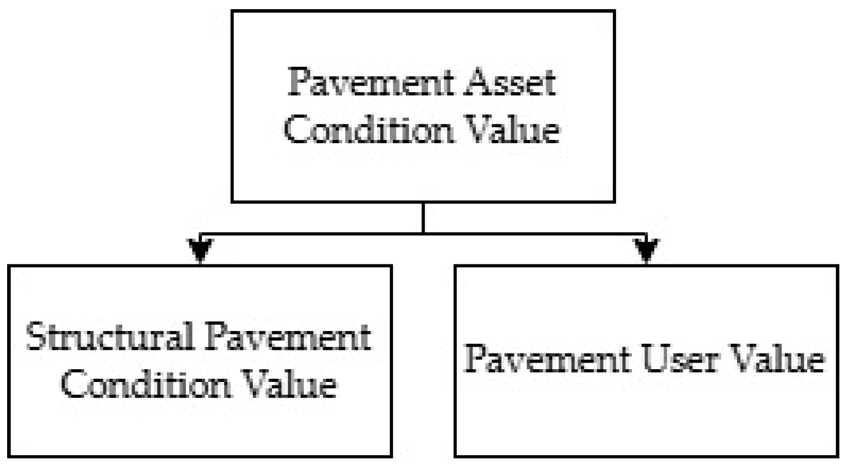
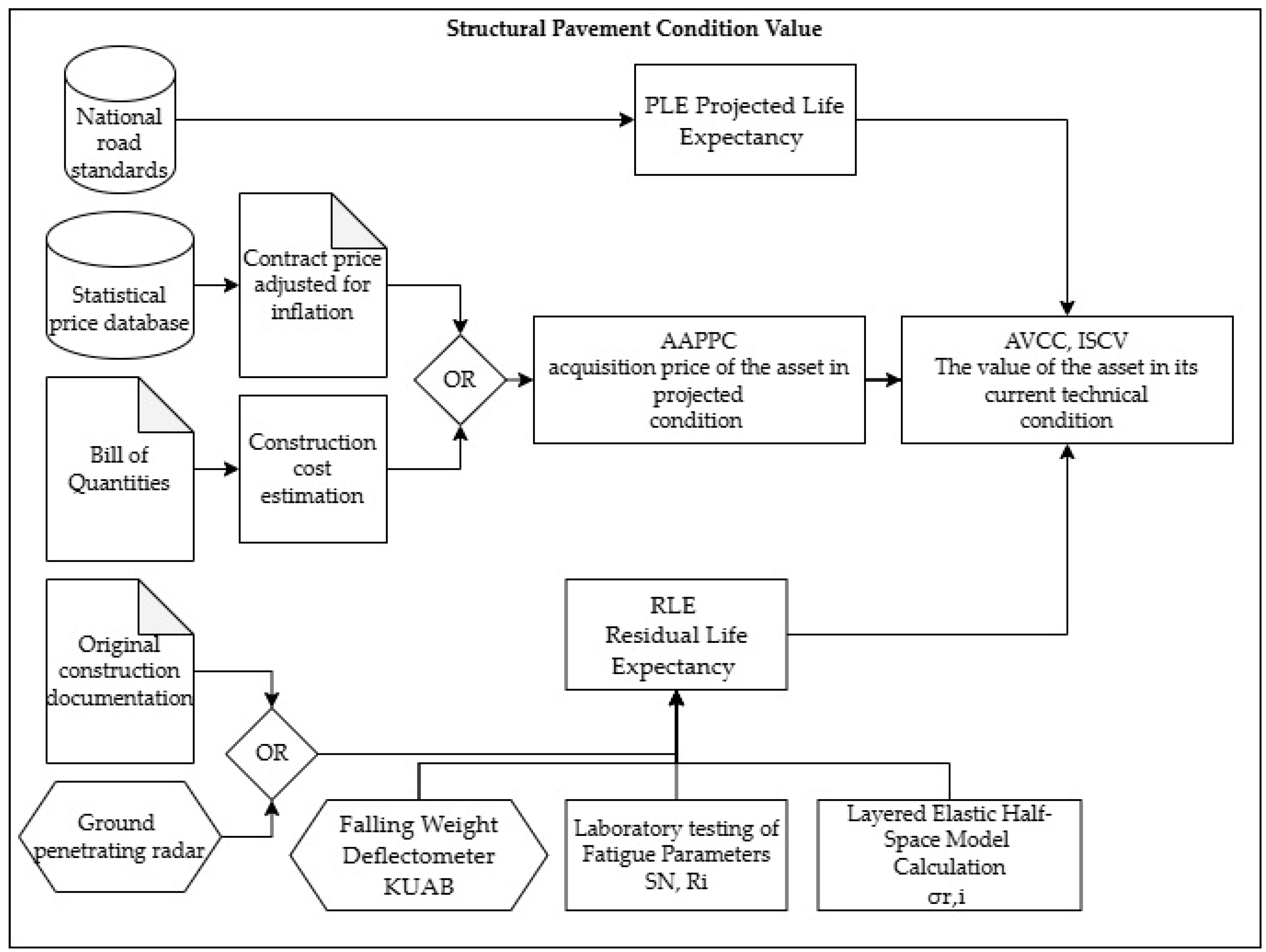
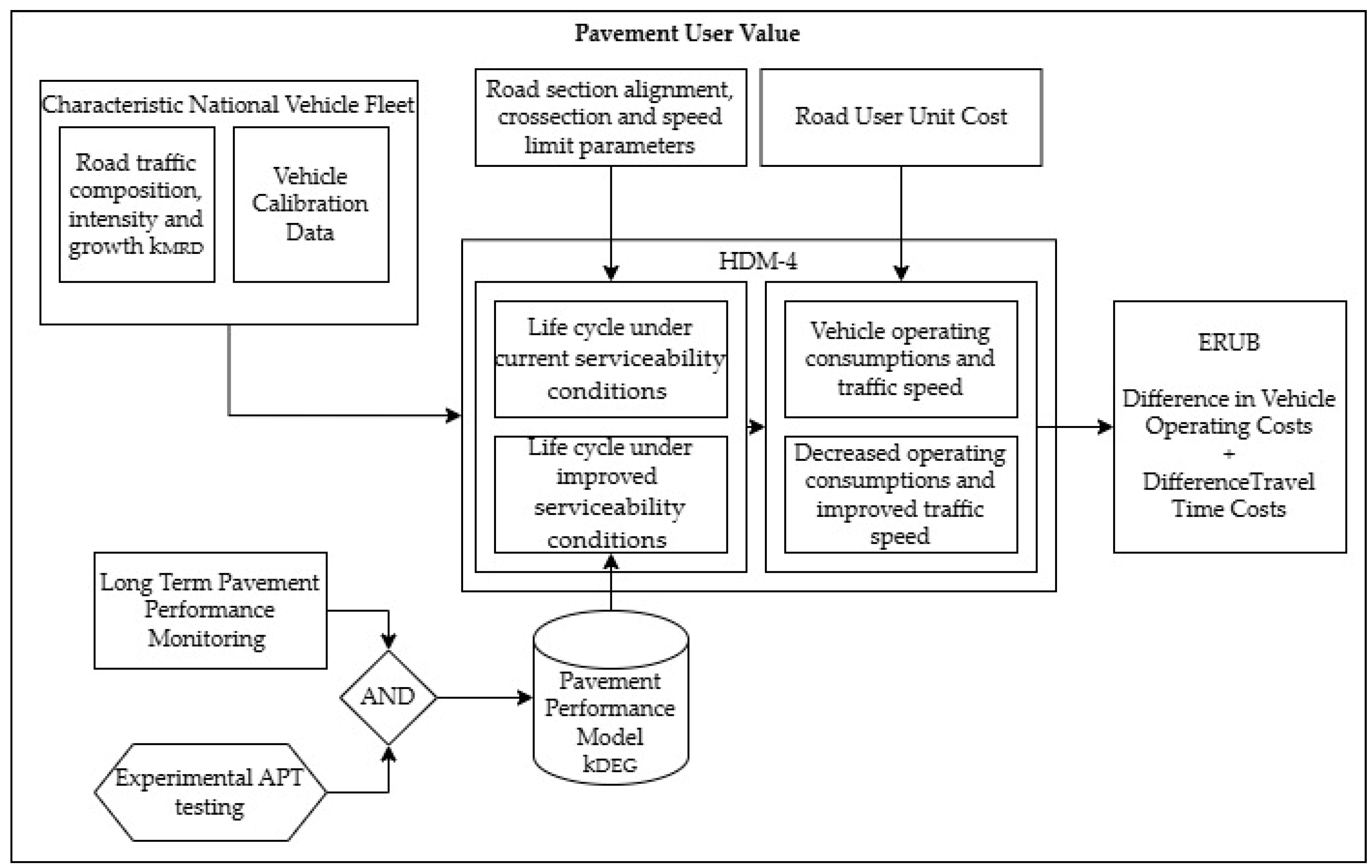
In this study, Pavement Asset Condition Value is defined as a function of two principal components: Structural Pavement Condition Value and Pavement User Value shown in Figure 1, Figure 2 and Figure 3 [17,18,19].

The Structural Pavement Condition Value reflects the ability of the pavement structure to withstand traffic and environmental loading within its life cycle [20,21]. It is derived from the current acquisition (or valuated) price of the pavement, which is reduced by the degree of wear. This wear is quantified through the concept of residual life, defined as the remaining service life relative to the projected (design) life of the pavement structure.

The residual life is determined based on mechanistic principles, including stress–strain conditions in a layered elastic half-space, material strength characteristics, and fatigue behavior of asphalt layers [22,23]. Since asphalt mixtures are composed of different binders, aggregates, and additives, their fatigue characteristics must be obtained experimentally. These parameters are highly dependent on material composition and local climatic conditions, making experimentally derived fatigue properties essential for accurate structural assessment [24,25,26].

The Pavement User Value is defined based on the relationship between pavement surface condition and road user costs. It reflects the economic impact of pavement performance on users, primarily through vehicle operating costs and travel time. The value is determined by comparing the user costs associated with the current pavement condition to those corresponding to a projected (ideal or rehabilitated) condition.

User costs include fuel and lubricant consumption, tire wear, vehicle maintenance, travel time losses, and accident-related costs. These parameters depend on multiple factors, such as traffic intensity, road alignment, gradient, intersection characteristics, and local defects. The calculation of user costs is typically performed using standardized models, such as those implemented in the World Bank’s HDM system, which provides calibrated coefficients for evaluating the relationship between pavement condition and vehicle operating costs [12,27].

The improvement in Pavement User Value is therefore expressed through the reduction in user costs achieved by implementing appropriate rehabilitation measures. These benefits can be further evaluated using economic appraisal methods, particularly Cost–Benefit Analysis (CBA), which enables the quantification of user-related benefits in monetary terms [28,29,30].

2.3. Role of Deterioration in Asset Value Development

A key characteristic of pavement assets is the continuous change in their condition due to deterioration processes. As pavement serviceability decreases over time, the corresponding asset value also declines. Therefore, accurate knowledge of deterioration processes and their impact on asset value is essential for effective pavement management.

The ability to predict the evolution of pavement condition is particularly important for the design of rehabilitation strategies and for determining the optimal timing of interventions within strategic maintenance planning. This requires a detailed understanding of the entire life cycle of pavement performance, from the initial condition after construction or rehabilitation to the point at which limit values defined by technical standards are reached.

However, the mathematical representation of deterioration processes requires comprehensive data covering the full operational life cycle of the pavement. Such data can only be obtained through a combination of experimental research and LTPPM.

In this context, the concept of Full-Life-Cycle deterioration models is introduced. These models describe pavement degradation from the initial condition to the defined terminal state and reduce the need to extrapolate beyond the range covered by the observations [31,32,33,34,35].

Consequently, a growing body of research has focused on integrating deterioration functions into proactive maintenance optimization frameworks [36,37], where condition predictions are used to support inspection scheduling, preventive maintenance policies, rehabilitation planning, and life-cycle cost minimization.

2.4. Implications for Pavement Rehabilitation Planning

The incorporation of Pavement Asset Condition Value into rehabilitation planning requires the determination of the optimal timing of maintenance interventions. This process is closely related to decision-making methods used in cross-asset allocation, where resources are allocated across infrastructure networks to maximize overall benefits [38,39].

Within this framework, rehabilitation measures are evaluated not only in terms of construction costs but also in terms of their impact on user costs and overall asset value. The objective is to identify the intervention strategy that maximizes the combined benefits of structural performance and user-related effects over the life cycle.

The determination of the optimal intervention time, often referred to as the “right time,” depends strongly on the accuracy of deterioration models. Inaccurate or incomplete models may lead to suboptimal decisions, resulting either in premature interventions or in excessive deterioration associated with increased user costs and higher rehabilitation expenses.

Therefore, deterioration models that adequately represent the relevant pavement performance stages are an important input for integrating pavement asset value into road asset management decision-making.

3. Structural Pavement Condition Value

The Structural Pavement Condition Value represents the technical component of the pavement asset value and reflects the ability of the pavement structure to withstand traffic and environmental loading throughout its life cycle. In accordance with the conceptual framework defined in Section 2, this value is expressed as a function of the current condition of the pavement relative to its projected (design) condition.

The current value of the pavement structure is defined based on its acquisition price, reduced by a coefficient representing the degree of structural deterioration. This coefficient is expressed as the ratio of residual life expectancy to projected life expectancy. The Structural Pavement Condition Value can therefore be formulated as

$${AV}_{CC}={AAP}_{PC}\times {\displaystyle \frac{RLE}{PLE}}$$

(1)

where

• AVCC is the value of the asset in its current technical condition [€];
• AAPPC is the acquisition price of the asset in projected condition [€];
• RLE is the residual life expectancy [years];
• PLE is the projected life expectancy [years].

For comparative and normalization purposes, it is also useful to express the Structural Pavement Condition Value in the form of an index representing the ratio of the current value to the projected value:

$$ISCV=1-{\displaystyle \frac{{\displaystyle {\sum }_{a=1}^{n_{assets}}}{\displaystyle {\sum }_{n=1}^{n_{sections}}}{\left({AAP}_{PC}-{AV}_{CC}\right)}_{a,n}}{{\displaystyle {\sum }_{a=1}^{n_{assets}}}{\displaystyle {\sum }_{n=1}^{n_{sections}}}{AAP}_{PCn,a}}}$$

(2)

where

• ISCV is the Index of Structural Condition Value [%].

The acquisition price in both current and projected conditions is determined based on available price databases of road administrations, typically derived from market prices obtained through public procurement processes.

3.1. Determination of Residual Life

The key parameter in the evaluation of structural condition is the residual life expectancy of the pavement structure. This parameter is determined based on mechanistic–empirical principles, considering stress–strain conditions in a layered elastic half-space, material strength properties, and fatigue behavior of asphalt layers [40].

The fundamental condition for structural performance is that the induced stresses in the pavement layers must not exceed the allowable material strength. In particular, the radial stress at the bottom of the asphalt layer must be lower than the flexural tensile strength of the material, adjusted for repeated loading through a fatigue coefficient [41]:

$${\sum }_{i=1}^n{Q}_i\times {\displaystyle \frac{{\delta }_{n,i}}{S_N\times R_{i,I}}}\le 1$$

(3)

where

• σ_r,i is the radial stress at the lower edge of the surfacing layer during period i [MPa];
• R_i is the flexural tensile strength of the material under the conditions of period i [MPa];
• S_N is the fatigue coefficient accounting for repeated loading effects.

The stress conditions vary depending on seasonal factors (e.g., winter and summer conditions), which influence material properties and loading response.

For the assessment of existing pavements within their life cycle, it is necessary to determine the actual mechanical properties of the structure, particularly the modulus of elasticity and material strength. These parameters can be obtained through in situ measurements of load-bearing capacity using a Falling Weight Deflectometer (FWD) [24,40].

The FWD applies an impact load to the pavement surface, inducing a deflection response. Using back-calculation methods based on layered elastic half-space theory, the elastic moduli of individual pavement layers can be derived from the measured deflection basin.

The fatigue characteristics of asphalt mixtures must be determined experimentally, as they depend on the specific composition of the materials used (binder type, aggregates, additives) and local climatic conditions [24,25]. Fatigue testing is typically performed by repeated bending of asphalt specimens in accordance with European standards [26].

3.2. Calculation of Residual Load-Carrying Capacity

The residual life of the pavement can be expressed in terms of the remaining number of allowable load repetitions, defined as Projected Axle Loads (PAL). This parameter is calculated using the following relationship [42]:

$$PAL={\left({\displaystyle \frac{\gamma \times {\epsilon }_6}{{\epsilon }_j}}\right)}^B$$

(4)

where

• PAL is the projected number of axle-load repetitions;
• ε₆ is the reference strain corresponding to 1.0 million load cycles derived from the fatigue curve [µm/m];
• ε_j is the relative strain at the bottom of the base course calculated using actual elastic moduli [µm/m];
• γ is the reliability factor of the fatigue test (typically γ = 1.6);
• B is the slope parameter of the fatigue curve (with B = −1/b).

This formulation allows the estimation of the remaining structural capacity of the pavement in terms of its ability to sustain future traffic loading.

3.3. Role of Structural Condition in Asset Value

The Structural Pavement Condition Value decreases progressively over time as a result of cumulative fatigue damage and material degradation. Its rate of decline depends on multiple factors, including traffic loading intensity, material properties, environmental conditions, and structural design.

Within the overall pavement asset value framework, the structural component represents the intrinsic capacity of the pavement to perform its function. However, it must be evaluated in conjunction with user-related performance, as structural adequacy alone does not guarantee acceptable serviceability.

Accurate estimation of residual life and structural condition is therefore essential not only for technical assessment but also for economic evaluation and decision-making. In particular, errors in estimating residual life may lead to incorrect valuation of the asset and suboptimal timing of rehabilitation interventions.

For this reason, the determination of Structural Pavement Condition Value must be based on experimentally validated parameters and reliable in situ measurements, ensuring consistency with the deterioration models and the overall asset management framework defined in this study.

4. Pavement User Value

Pavement User Value represents the economic component of the pavement asset value and reflects the impact of pavement condition on road users. In accordance with the framework defined in Section 2, it is expressed through the relationship between pavement serviceability and road user costs, which are directly influenced by surface characteristics, particularly pavement roughness.

Pavement serviceability is primarily quantified using the International Roughness Index (IRI), which serves as a key indicator of surface condition. As pavement deterioration progresses, roughness increases, leading to higher vehicle operating costs and travel time losses. Pavement User Value may be expressed either in monetary terms, as road user benefits (RUB), or in the form of a dimensionless Index of Pavement User Value (IPUV). The monetary representation, discussed in the following subsections, is generally preferred because it directly quantifies the economic benefits resulting from improved pavement serviceability and allows compatibility with Life-Cycle Cost Analysis (LCCA) and Cost–Benefit Analysis (CBA) frameworks.

However, in addition to the monetary representation, Pavement User Value may also be expressed by means of the following index:

$$\mathrm{I}\mathrm{P}\mathrm{U}\mathrm{V}={\displaystyle \frac{{\mathrm{RUB}}_{\mathrm{cs}}}{{\mathrm{RUB}}_{\mathrm{dps}}}} \times 100$$

(5)

where

• IPUV is the Index of Pavement User Value [%];
• RUB_CS is the road user costs under current serviceability conditions [€];
• RUB_dps is the road user costs under projected (design) serviceability conditions [€].

Unlike Pavement User Value expressed in monetary units, the IPUV represents a dimensionless indicator describing the relative effectiveness of rehabilitation measures. Its primary purpose is not to quantify absolute economic benefits but rather to facilitate comparisons among alternative investment scenarios.

The index is particularly useful when evaluating multiple rehabilitation alternatives or performing network-level optimization and cross-asset allocation. Since absolute road user benefits are strongly influenced by traffic volume and road section length, relying solely on monetary values may systematically favor larger road networks. In contrast, IPUV reflects the proportional improvement achieved by a given intervention and therefore enables a more equitable comparison between road sections or road agencies managing networks of different sizes. Consequently, IPUV may serve as a suitable input variable for optimization procedures and AI-driven decision-support systems involving multiple investment alternatives.

4.1. Road User Costs

Road user costs represent the total expenses incurred by road users due to the operation of vehicles and travel on a given pavement section. These costs are typically divided into two main categories:

• Vehicle operating costs (VOC);
• Travel time costs.

Vehicle operating costs include fuel and lubricant consumption, tire wear, vehicle maintenance and repairs and spare parts consumption.

Travel time costs include crew travel time, passenger travel time and cargo-related time costs.

In addition, accident-related costs may also be considered depending on the level of analysis. The magnitude of these costs depends on multiple factors, including traffic intensity, road alignment, gradient, intersection density, and the presence of local defects or irregularities.

The calculation of road user costs is typically performed using standardized models, such as those implemented in the World Bank’s Highway Development and Management (HDM) system. These models provide calibrated relationships between pavement condition (e.g., IRI) and user costs, allowing for consistent evaluation of the economic impact of pavement deterioration [8,32,33].

4.2. Evaluation of User Benefits

The improvement in Pavement User Value resulting from rehabilitation measures can be expressed through the reduction in user costs achieved by improving pavement serviceability. This benefit can be quantified over the life cycle of the pavement using the following relationship:

$$\mathrm{E}\mathrm{R}\mathrm{U}\mathrm{B}=\sum _{\mathrm{t}=1}({\left({\mathrm{NRUC}}_{\mathrm{cs}}-{ \mathrm{NRUC}}_{\mathrm{is}}\right)\times {\mathrm{k}}_{\mathrm{DEG}} \times {\mathrm{k}}_{\mathrm{MRD}})}^{\mathrm{t}}$$

(6)

$$k_{DEG}=1-\mathrm{A}{\left({\displaystyle \frac{\mathrm{t}}{\mathrm{Tt}}}\right)}^{\mathrm{B}}$$

(7)

where

• ERUB is the expected road user benefits [€];
• NRUC_cs is the net road user costs under current serviceability conditions [€];
• NRUC_is is the net road user costs under improved serviceability conditions [€];
• k_MRD is the annual traffic growth coefficient;
• k_DEG is the degradation coefficient based on deterioration models;
• t is the time in years from the beginning of the pavement life cycle;
• Tt is the total expected service life of the pavement [years];
• A is a parameter expressing the type of pavement and materials used (0 < A ≤ 1);
• B is a pavement design parameter (0.2 < B ≤ 6.0).

This formulation allows the evaluation of cumulative user benefits over time, taking into account traffic growth and the progressive deterioration of pavement condition.

4.3. Integration into Economic Evaluation

From an asset management perspective, Pavement User Value plays a crucial role in evaluating the effectiveness of rehabilitation strategies. Improvements in pavement condition lead to reductions in user costs, which represent direct economic benefits for society.

These benefits are typically assessed using Cost–Benefit Analysis (CBA), which enables the comparison of investment costs with the resulting savings in user costs [34,35,36]. Within this framework, Pavement User Value represents a key input parameter for the quantification of benefits associated with different rehabilitation scenarios.

The integration of user costs into the asset value framework ensures that decision-making is not based solely on structural condition but also accounts for the economic impact on road users. This is particularly important in cases where surface deterioration significantly affects operating conditions, even if the structural capacity of the pavement remains adequate.

4.4. Role of Pavement User Value in Asset Management

Pavement User Value decreases over time as pavement roughness increases due to deterioration processes. However, this decrease is not linear, as it is directly influenced by the nonlinear evolution of surface condition parameters, particularly IRI.

The accurate representation of this relationship is therefore dependent on the quality of deterioration models, which define how pavement condition evolves over time. In combination with the Structural Pavement Condition Value, Pavement User Value forms a comprehensive basis for evaluating the overall pavement asset value and for determining optimal maintenance and rehabilitation strategies.

Within the proposed framework, Pavement User Value provides a direct link between technical condition and economic performance, enabling more informed and efficient decision-making in road asset management systems.

5. Full-Life-Cycle Deterioration Models

The pavement asset value, as defined in Section 2, Section 3 and Section 4, is directly influenced by the evolution of pavement serviceability over time. User costs increase with deteriorating pavement serviceability [32]. As pavement condition deteriorates due to traffic loading and environmental effects, both the Structural Pavement Condition Value and the Pavement User Value decrease. Therefore, an accurate representation of deterioration processes is essential for reliable asset valuation and for determining optimal rehabilitation strategies.

Over the complete pavement life cycle, deterioration frequently exhibits nonlinear behavior and changes in the rate of degradation. The rate of degradation varies throughout the life cycle and depends on multiple factors, including material properties, structural design, traffic intensity, and climatic conditions. Consequently, the applicability of models calibrated from partial-life-cycle data should generally be restricted to the observed range unless their extrapolation has been independently validated.

To address this limitation, the concept of Full-Life-Cycle deterioration models is introduced. These models describe the full progression of pavement degradation from the initial condition (after construction or rehabilitation) to the terminal state defined by limit values prescribed in technical standards. The development of such models requires comprehensive data covering the entire life cycle of pavement performance.

The derivation of Full-Life-Cycle deterioration models in this study is based on two primary sources:

• Experimental measurements obtained through accelerated pavement testing (APT);
• Long-term monitoring data collected on real road sections within the national road database.

5.1. Experimental Determination of Deterioration

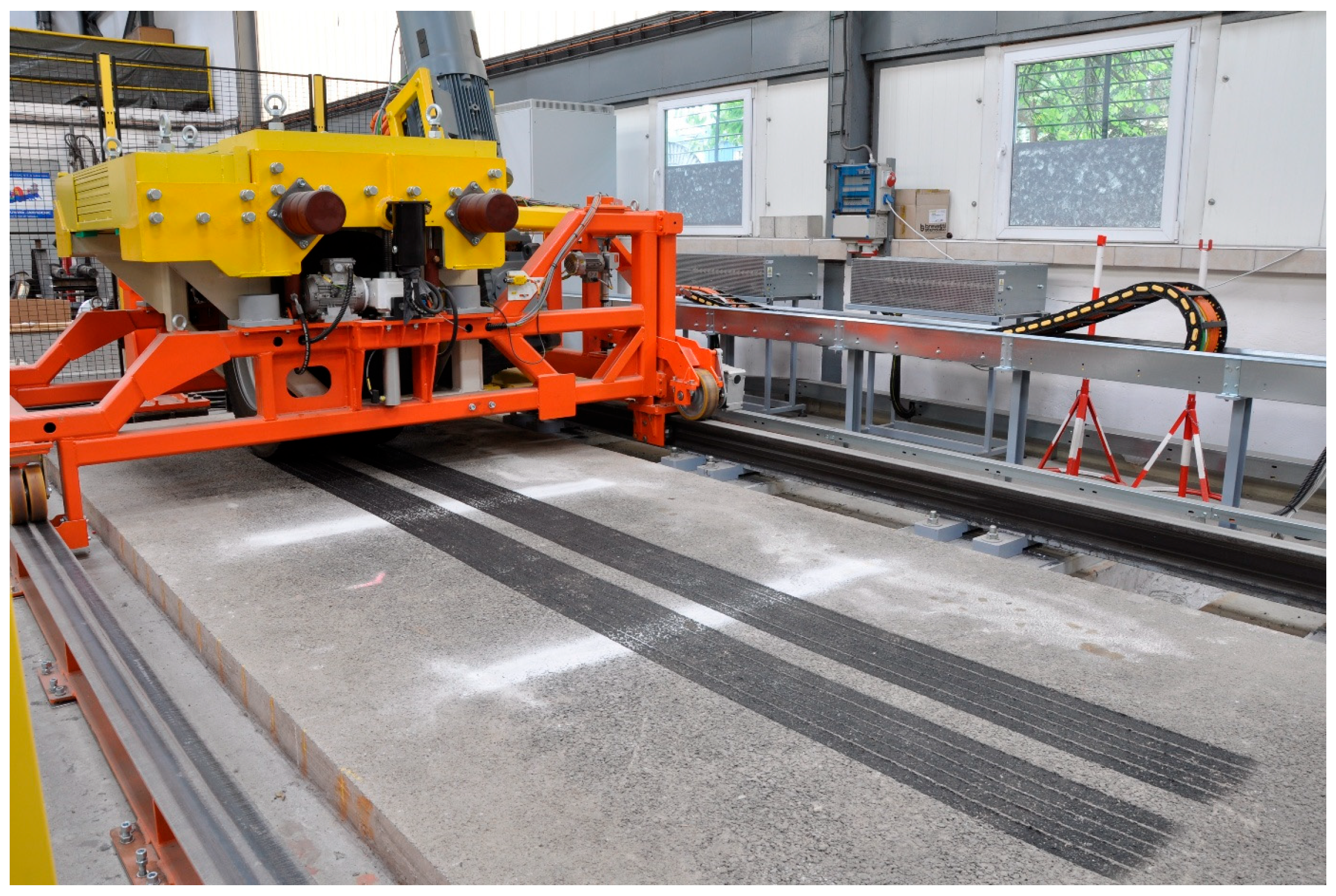
An experimental facility for accelerated pavement testing (APT), was designed and constructed at the University of Žilina as an original prototype, see Figure 4. The testing device applies traffic loading equivalent to standard axle loads in a 1:1 ratio, while the tested pavement structure is designed according to standard construction of first-class roads.

The facility operates continuously (24 h per day), allowing the accumulation of a large number of load repetitions within a relatively short time period. In the current experiment, approximately 1.8 million axle-load repetitions have been achieved, enabling the deterioration process to be observed up to the limit values defined by technical standards.

Deformation measurements are performed using precise leveling techniques and advanced road scanning systems, which allow the processing of data in the form of point clouds. This provides detailed information on the development of pavement surface parameters, particularly transverse deformation (rutting).

The main advantage of the experimental approach is the ability to observe the full deterioration process under controlled conditions, where external influences such as climatic effects can be minimized. However, this also leads to higher variability in the measured data due to the intensity of loading applied over a shorter time period.

5.2. Long-Term Pavement Performance Monitoring

In addition to experimental measurements, LTPPM is used. These data are collected within the national road database over a period exceeding 20 years.

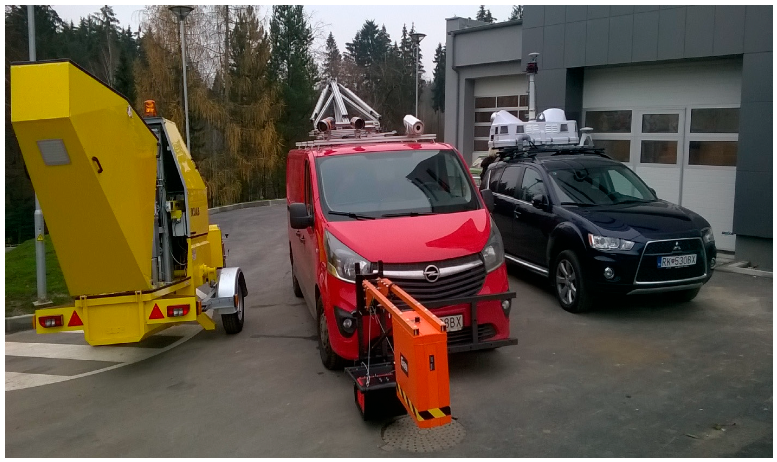
Measurements are performed using profilograph systems (e.g., Profilograph GE) equipped with laser sensors, enabling accurate determination of pavement roughness parameters. These measurements are continuously supplemented by additional diagnostic equipment developed at the University of Žilina, see Figure 5, allowing for a comprehensive assessment of pavement serviceability and structural condition.

The long-term monitored section used in this study is located on a first-class road (I/64). The available data provide information on the evolution of pavement condition under real traffic and environmental conditions.

Compared to experimental measurements, long-term monitoring data exhibit smoother progression of deterioration, as they reflect the combined effects of traffic loading and environmental influences over extended periods.

5.3. Modeling of Transverse Uneveness

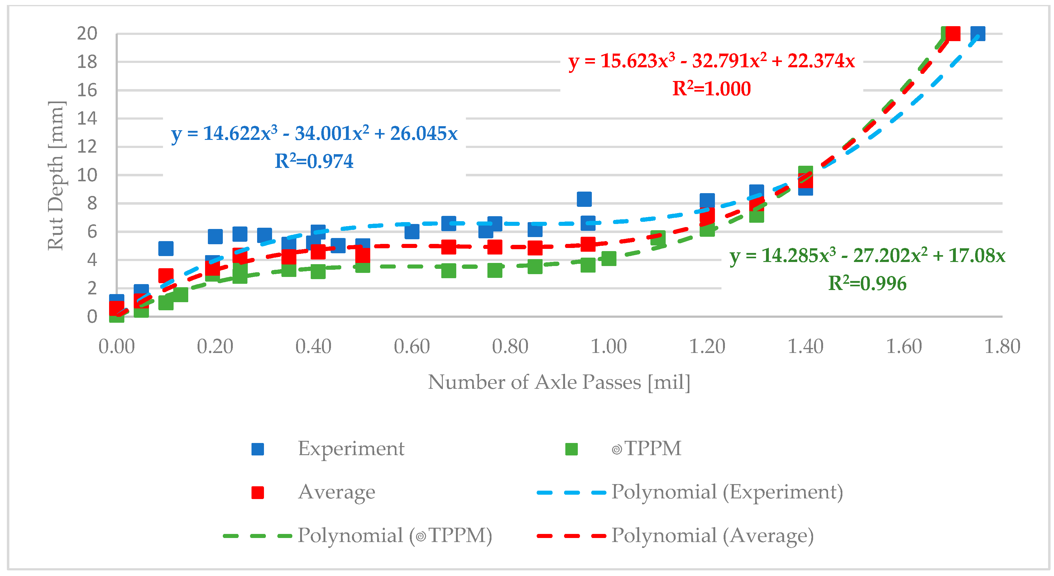
Based on the performed measurements on experimental sections, where repeated loading enabled the achievement of limit values, it is possible to mathematically express the development of transverse roughness using Full-Life-Cycle deterioration models. These models were derived both from experimental measurements and from LTPPM on road sections. The results are presented in Figure 6.

Figure 6 shows the progression of rut depth in millimeters as a function of the number of axle passes. The graph combines data from two types of measurements of variable parameters: data from an experimental measurement conducted at the University of Žilina and data from the LTPPM road section I/64. The objective of the modeling was to determine and compare the results of both types of measurement upon reaching the limit value of 20 mm according to National standards (TP 056) [41], at which point the roadway, in terms of the variable parameter assessment, is deemed unsuitable for traffic.

When comparing both datasets (experimental and LTPPM), we can conclude that the experimental measurements exhibit higher values of variance, which is caused by controlled and intensive loading over a shorter observation period. LTPPM data show a more gradual increase, which, at high passage counts, reaches comparable or higher rut depth values than the experimental measurements. The difference between the models is also due to the fact that experimental measurements (accelerated pavement testing) eliminate external influences, such as degradation caused by climatic conditions. The measured development of transverse unevenness exhibited a nonlinear trajectory containing an initial increase, a period of relative stabilization, and subsequent acceleration. Among the functional forms evaluated during model development, the polynomial function provided a suitable representation of this observed trajectory and was therefore selected for the experimental and LTPPM datasets. The final rut degradation function was derived as an average function of experimental and LTPPM data, the regression analysis is shown in

Table 2. Regression analysis of average rut depth degradation model.

Regression Statistics
Multiple R						1
R Square						1
Adjusted R Square						0.961538462
Standard Error						2.21877 × 10−5
Observations						29
	df		SS		MS	F	Significance F
Regression	3		1791.469275		597.1564251	1.21301 × 1012	1.1899 × 10−139
Residual	26		1.27996 × 10−8		4.92292 × 10−10
Total	29		1791.469275
	Coefficients	Standard Error	t Stat	p-value	Lower 95%	Upper 95%	Lower 95.0%	Upper 95.0%
X Variable 1	15.62295615	2.9026 × 10−5	538239.469	3.7981 × 10−132	15.62289648	15.62301581	15.62289648	15.62301581
X Variable 2	−32.79092543	6.84122 × 10−5	−479313.7876	7.7413 × 10−131	−32.79106605	−32.79078481	−32.79106605	−32.79078481
X Variable 3	22.37397293	3.73697 × 10−5	598720.3461	2.3829 × 10−133	22.37389612	22.37404975	22.37389612	22.37404975
$$P\left(x\right)P\left(x\right)=15.6229x^3-32.7909x^2+22.37397x$$ (8)

.

The resulting residual axle pass counts from the individual models are shown in Table 2. The degradation model is shown in Equation (8).

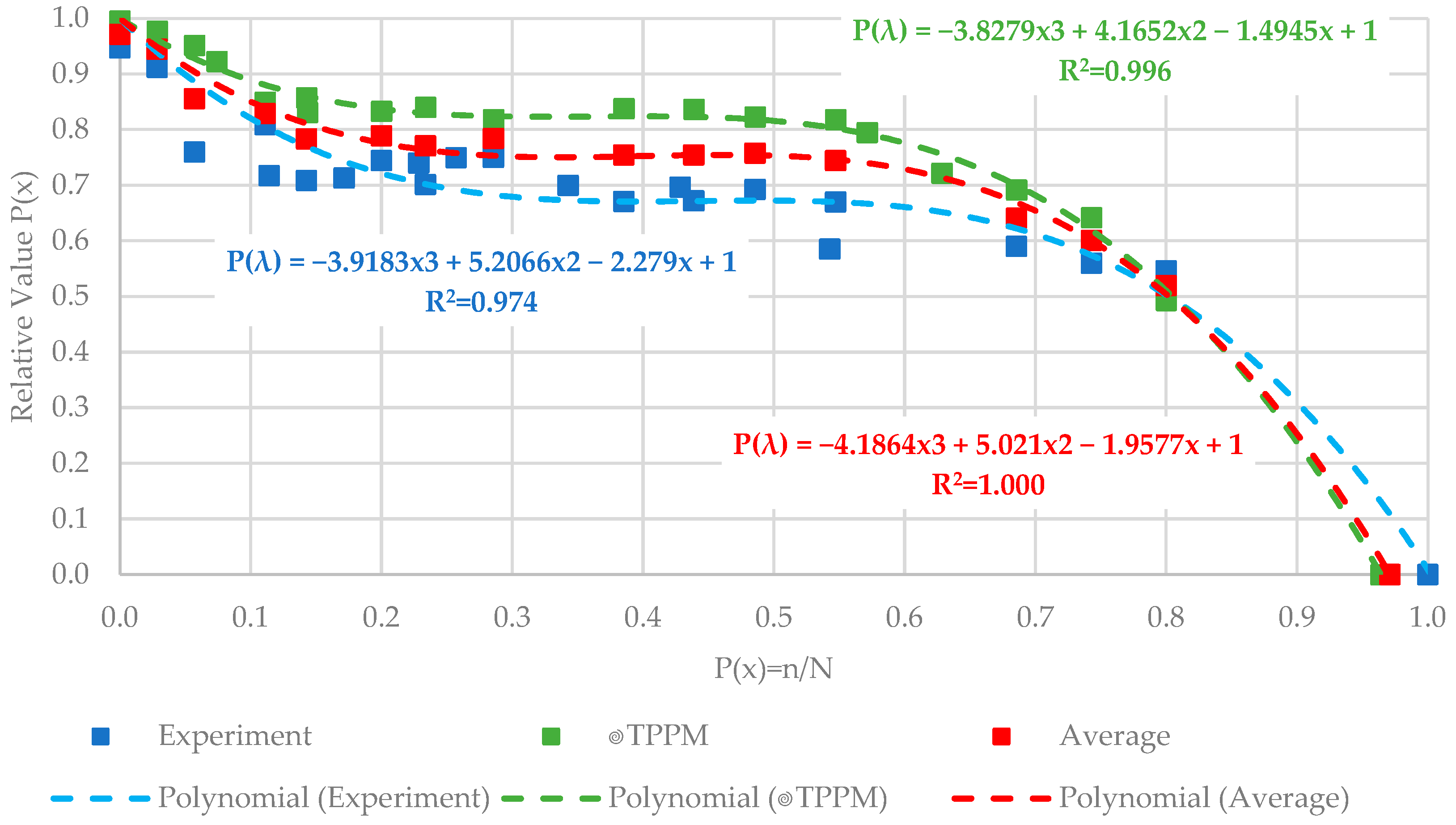
The deterioration models presented in this study were initially expressed as a function of the cumulative number of design axle loads. However, such a formulation limits the direct applicability of the models to pavement structures designed for identical traffic loading conditions. Since pavement structures are commonly designed for different traffic categories and different projected numbers of axle-load repetitions, a normalized representation of deterioration development was introduced. For this purpose, the horizontal axis of the deterioration functions was reformulated using a life fraction parameter:

$$\mathsf{\lambda }={\displaystyle \frac{n}{N}}$$

(9)

where

• λ is life fraction parameter;
• n is the cumulative number of DAL;
• N is the projected number of DAL repetitions for which the pavement structure was originally designed.

The introduction of life fraction parameter $\mathsf{\lambda }$ is important because it enables deterioration models to be applied universally across pavement structures designed for different traffic loading levels. Instead of expressing deterioration as an absolute number of axle-load repetitions, the pavement condition is represented within a normalized interval from 0 to 1 (or equivalently from 0% to 100% of the projected traffic loading capacity).

This relative formulation significantly improves the comparability of deterioration behavior between different pavement structures and allows the development of generalized Full-Life-Cycle deterioration models applicable at both project and network levels. At the same time, it enables easier integration of deterioration models into pavement management systems, asset valuation procedures, and cross-asset allocation decision-making processes, where normalized indicators are required for comparing assets with different structural and traffic characteristics. The degradation model in this relative form is shown in Equation (10) and Figure 7.

$$P\left(\mathsf{\lambda }\right)=-4.1864x^3+5.021x^2-1.9577x+1$$

(10)

It should be noted that the normalized Full-Life-Cycle deterioration model was not derived directly from experimental measurements. Instead, it was obtained by transforming the previously established and experimentally validated deterioration model into a normalized form using the life fraction parameter λ. Consequently, the reported regression statistics characterize the quality of the mathematical approximation rather than the uncertainty associated with the original measurements.

5.4. Evaluation of Deterioration Modeling Results

The graphical evaluation indicates that a single constant deterioration rate would not adequately represent the observed development of unevenness over the complete investigated life cycle. The analysis shows that both sets of unevenness exhibit a nonlinear progression, characterized by a relatively rapid increase in the initial stage, primarily due to material consolidation. This is followed by a phase of partial stabilization, after which a significant acceleration of deterioration occurs at a certain stage of the pavement life cycle.

Identifying this transition point provides an important input for estimating the appropriate timing of rehabilitation interventions, as exceeding this threshold results in a rapid increase in maintenance and repair costs, as well as a significant decline in pavement serviceability and operational performance.

The results therefore highlight the necessity of identifying the optimal intervention moment, at which rehabilitation measures are both technologically appropriate and economically efficient.

A thorough understanding of deterioration-curve development, together with an appropriately calibrated model, provides an important basis for maintenance planning, service-life assessment, and allocation of financial resources.

6. Case Study

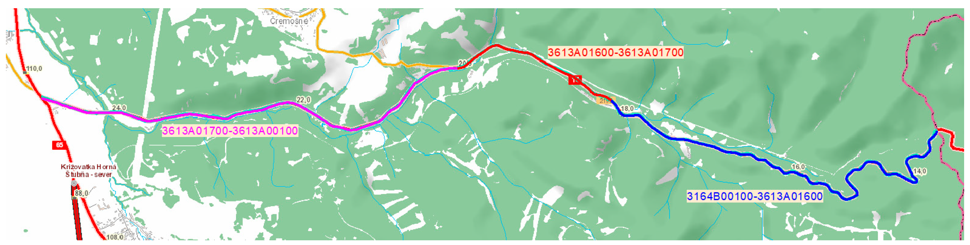
The case study focuses on a road infrastructure asset I/14 (11.526 km) classified as a first class road (trunk road), category C9.5/90, which represents a regionally important transport connection. For the purposes of analysis, the road section was divided into three technically homogeneous segments, as shown in Figure 8 and

Table 3. Basic characteristics of the homogeneous road sections included in the case study.

No.	Nod Identification System	Category	Pavement	Length [km]	Width	Curvature [°/km]	Rise and Fall [%]	No. Lanes	Speed Limit [km/h]
01	3164B00100-3613A01600	C9.5	Flexible	4.95	9.5	370	4	2	90
02	3613A01600-3613A01700	C9.5	Flexible	1.605	9.5	125	2.5	2	90
03	3613A01700-3613A00100	C9.5	Flexible	4.971	9.5	100	1.5	2	90

.

A comprehensive diagnostic survey was carried out to assess the current condition of the pavement and to obtain input data for the design of the rehabilitation technology. The applied diagnostic methods included videocar inspection, profilograph measurements, Falling Weight Deflectometer (FWD KUAB), and ground-penetrating radar (GPR).

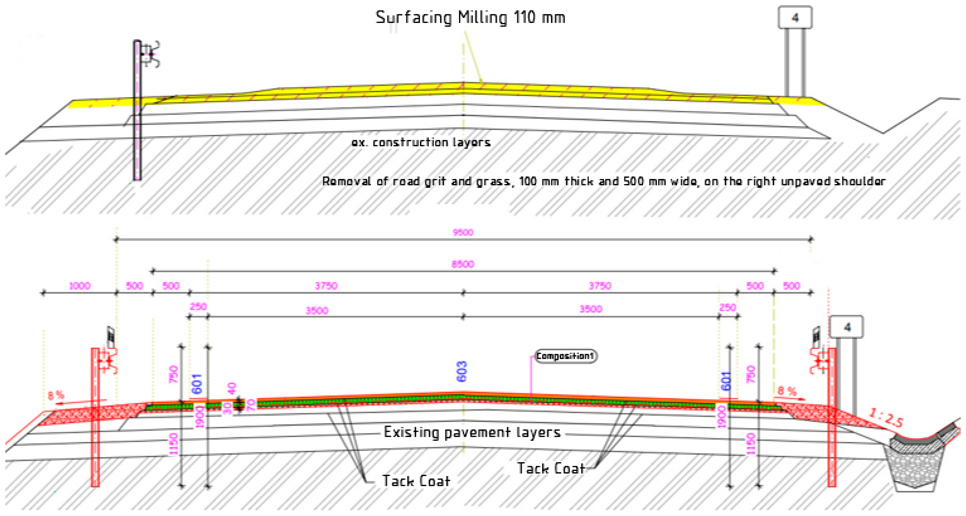
Based on the national methodologies TP024, TP031, and TP033, the residual service life of the existing pavement structure was determined to be 3 years. Consequently, a rehabilitation strategy with a design life of 20 years was designed (4.2 × 10⁶ design axle loads), consisting of a Mill and Replace technology (see Figure 9). The milling depth was defined as 110 mm, corresponding to the removal of the structurally inadequate and significantly deteriorated surfacing layers.

6.1. Structural Pavement Condition Value

The replacement surfacing is defined by the composition of individual layers presented in

Table 4. New surfacing design.

No.	Description	Units	Quantity	Unit Price [€]	Value [€]
1	Wearing course—Asphalt concrete AC 11 O, lane width > 3 m, using polymer-modified bitumen (Class I), compacted thickness 40 mm	m2	97,971	14	1,337,304
2	Tack coat—Bituminous emulsion without aggregate spreading, application rate 0.80 kg/m2	m2	117,565	1	89,350
3	Binder course—Asphalt concrete AC 22 L, lane width > 3 m, using polymer-modified bitumen (Class I), compacted thickness 70 mm	m2	98,202	23	2,227,210
4	Tack coat—Bituminous emulsion without aggregate spreading, application rate 0.80 kg/m2	m2	118,257	1	89,875
5	Asphalt surfacing—Stone Mastic Asphalt SMA 8 O (fine-graded), Class I modified binder, compacted thickness 30 mm, lane width > 3 m	m2	99,124	10	1,032,868
6	Tack coat—Bituminous emulsion without aggregate spreading, application rate 0.80 kg/m2	m2	118,948	1	90,401
	SUM			∑	4,867,008

. This table also includes the construction cost of the new pavement structure, which represents the first component of the Structural Pavement Condition Value. Detailed breakdown of cost composition of each pavement layer is in

Table 5. Cost breakdown for each layer.

Layer No.	Material [€]	Wages [€]	Insurance [€]	Machinery [€]	Overheads [€]	Profit [€]	Material Weight [Tons]	Workload [Normative Hours]
1	1,188,976	43,313	15,679	34,399	36,576	18,195	10,163	3674
2	78,627	3274	1185	2247	2765	1326	95	317
3	1,978,564	71,780	25,984	59,829	60,614	30,549	17,826	6088
4	79,090	3294	1192	2260	2781	1334	96	319
5	905,590	38,214	13,833	26,989	32,269	15,583	7187	3241
6	79,552	3313	1199	2273	2798	1342	96	321
SUM ∑	4,310,398	163,188	59,074	127,998	137,803	68,329	35,463	13,962

.

The second component of the Structural Pavement Condition Value is represented by the residual value of the subbase layer subgrade layer and the road embankment. Ground-penetrating radar diagnostics confirmed that the subbase layers remain geometrically stable. Visual inspection further indicated that the embankment shows no signs of instability, such as landslides or significant deformations. As the original construction documentation was not available, the acquisition prices of newly constructed subbase layers and embankment were determined based on current reference values, as presented in

Table 6. Cost breakdown for subbase, subgrade and embankment.

No.	Description	Units	Quantity	Unit Price [€]	Value [€]
1	Cement-bound granular subbase (CBGM C 5/6), with spreading and compaction, compacted thickness 150 mm	m2	126,786	15	0.5 × 1,930,951
2	Crushed aggregate subgrade, with spreading and compaction, compacted thickness 220 mm	m2	138,312	14	1,955,732
4	Earthworks—excavation	m3	69,156	4	269,708
3	Earthworks—embankment	m3	69,156	7	496,540

. The residual (replacement) value of these structural components was estimated as 50% of the value of newly constructed subbase layers and 100% of the value of subgrade and embankment. These values represent the second component of the Structural Pavement Condition Value.

The AAPPC (acquisition price of the asset in projected condition) for the given case study is calculated using Equation (11). After substitution, the resulting value is €8,071,726.

$$\begin{gathered} {AAP}_{PC}={\displaystyle \sum _{i=1}^n}{NPL}_v+\left({SB}_v\times {ksb}_{rv}\right)+\left({SG}_v\times {ksg}_{rv}\right)+\left(E_v\times {ke}_{rv}\right) \\ {AAP}_{PC}=4,867,008+\left(1,930,951\times 0.5\right)+\left(\mathrm{1,955,732}\times 1.0\right)+\left(\mathrm{766,248}\times 1.0\right) \\ {AAP}_{PC}=8,071,726\mathrm{€} \end{gathered}$$

(11)

where

• AAP_PC is the acquisition price of the asset in projected condition [€];
• NPL_v is the acquisition price of new pavement layer i [€];
• SB_v is the value of existing subbase [€];
• ksb_rv is the residual value coefficient for existing subbase (ksb_rv = 0.5);
• SG_v is the value of existing subgrade [€];
• ksg_rv is the residual value coefficient for existing subgrade (ksg_rv = 1.0);
• E_v is the value of existing embankment [€];
• ke_rv is the residual value coefficient for existing embankment (ke_rv = 1.0);
• n is the number of new pavement layers.

By substituting in Equation (12), AAP_PC = €8,071,726, the residual life expectancy is 3 years, and the projected life expectancy is 20 years, while the AV_CC (value of the asset in its current technical condition) is determined as €1,210,759. The corresponding ISCV (Index of Structural Condition Value) is 0.15, i.e., 15%.

$$\begin{gathered} {AV}_{CC}={AAP}_{PC}\times {\displaystyle \frac{RLE}{PLE}} \\ {AV}_{CC}=8,071,726\times {\displaystyle \frac{3}{20}} \\ {AV}_{CC}=1,210,759 € \\ ISCV=1-{\displaystyle \frac{{\displaystyle {\sum }_{a=1}^{n_{assets}}}{\displaystyle {\sum }_{n=1}^{n_{sections}}}{\left({AAP}_{PC}-{AV}_{CC}\right)}_{a,n}}{{\displaystyle {\sum }_{a=1}^{n_{assets}}}{\displaystyle {\sum }_{n=1}^{n_{sections}}}{AAP}_{PC n,a}}} \\ ISCV=1-{\displaystyle \frac{8,071,726-1,210,759}{8,071,726}} \\ ISCV=0.15 \end{gathered}$$

(12)

After the rehabilitation is carried out, the AV_CC increases to €8,071,726, and the ISCV reaches a value of 1.0, i.e., 100%.

6.2. Pavement User Value

For the calculation of Pavement User Value, it was necessary to model the selected road sections using the HDM-4 software. HDM-4 was selected because it is an internationally established framework for road management and economic appraisal and because its deterioration, vehicle operating cost, travel time, and maintenance models can be calibrated to local or regional conditions. The numerical road user benefits are therefore dependent on the selected HDM-4 calibration and on the unit costs, vehicle fleet characteristics, traffic composition, and economic parameters applied in the analysis. The use of an alternative national user–cost model or a different regional calibration could change the absolute monetary values. Nevertheless, it would not alter the fundamental methodological principle proposed in this paper: the change in road asset performance is converted into a change in road user costs, and this change is subsequently incorporated into the valuation of the road asset.

A key input in the HDM-4 calculation was the application of the full-life-cycle pavement deterioration models described in Section 5.3, which directly influence user costs associated with vehicle operation on pavements with a given level of deterioration derived from these models. Two scenarios were analyzed within the HDM-4 framework. The first scenario, referred to as “Do Something,” represents the life cycle of a pavement rehabilitated using the proposed repair technology designed for a service life of 20 years, i.e., 4.2 × 10⁶ design axle loads as described in Section 6. The second scenario, referred to as “Do Nothing” (or “Do Minimum”), represents a 20-year period of pavement operation during which the road authority performs only essential maintenance activities to ensure basic trafficability. These interventions do not address permanent (plastic) deformations and therefore do not improve ride quality or reduce user costs. As a result, user costs in this scenario remain at levels corresponding to the current deteriorated condition of the pavement.

Traffic volumes used as input parameters are presented in

Table 7. Traffic composition in annual average daily traffic (EDAL = Equivalent Design Axle Load).

Vehicle	Small Two-Axle Rigid Truck (Approx. <3.5 Tons), 0.5 EDAL	Medium Two-Axle Rigid Truck (>3.5 Tons), 1.4 EDAL	Medium Passenger Cars, 0 EDAL	Multi-Axle or Large Two-Axle Bus, 1.8 EDAL	Articulated Truck or Truck with Drawbar Trailer, 2.4 EDAL	Multi-Axle Rigid Truck, 2.7 EDAL	Total AADT
AADT	224	84	2191	12	105	25	2641

; this table also includes Equivalent Design Axle Loads for each type of vehicle. The calculated outputs are summarized in

Table 8. Annual road user cost for both scenarios, mil. €.

Year	I/14—Do Something			I/14—Do Nothing			Discounted Annual Total ROC
	Annual VOC	Annual TTC	Annual Total ROC	Annual VOC	Annual TTC	Annual Total ROC	Do Something	Do Nothing
2026	3.727	2.606	6.333	4.812	3.491	8.303	6.333	8.303
2027	3.730	2.606	6.336	4.812	3.491	8.303	6.035	7.908
2028	3.733	2.607	6.339	4.812	3.491	8.303	5.750	7.531
2029	3.735	2.607	6.342	4.812	3.491	8.303	5.478	7.172
2030	3.737	2.607	6.343	4.812	3.491	8.303	5.219	6.831
2031	3.738	2.607	6.345	4.812	3.491	8.303	4.971	6.506
2032	3.739	2.607	6.346	4.812	3.491	8.303	4.735	6.196
2033	3.739	2.607	6.346	4.812	3.491	8.303	4.510	5.901
2034	3.739	2.607	6.346	4.812	3.491	8.303	4.295	5.620
2035	3.740	2.607	6.347	4.812	3.491	8.303	4.091	5.352
2036	3.740	2.607	6.347	4.812	3.491	8.303	3.897	5.097
2037	3.742	2.607	6.349	4.812	3.491	8.303	3.712	4.855
2038	3.747	2.607	6.355	4.812	3.491	8.303	3.539	4.623
2039	3.766	2.608	6.374	4.812	3.491	8.303	3.380	4.403
2040	3.827	2.609	6.436	4.812	3.491	8.303	3.251	4.194
2041	3.911	2.613	6.523	4.812	3.491	8.303	3.138	3.994
2042	4.016	2.624	6.640	4.812	3.491	8.303	3.042	3.804
2043	4.154	2.660	6.814	4.812	3.491	8.303	2.973	3.623
2044	4.321	2.769	7.090	4.812	3.491	8.303	2.946	3.450
2045	4.532	3.032	7.563	4.812	3.491	8.303	2.993	3.286
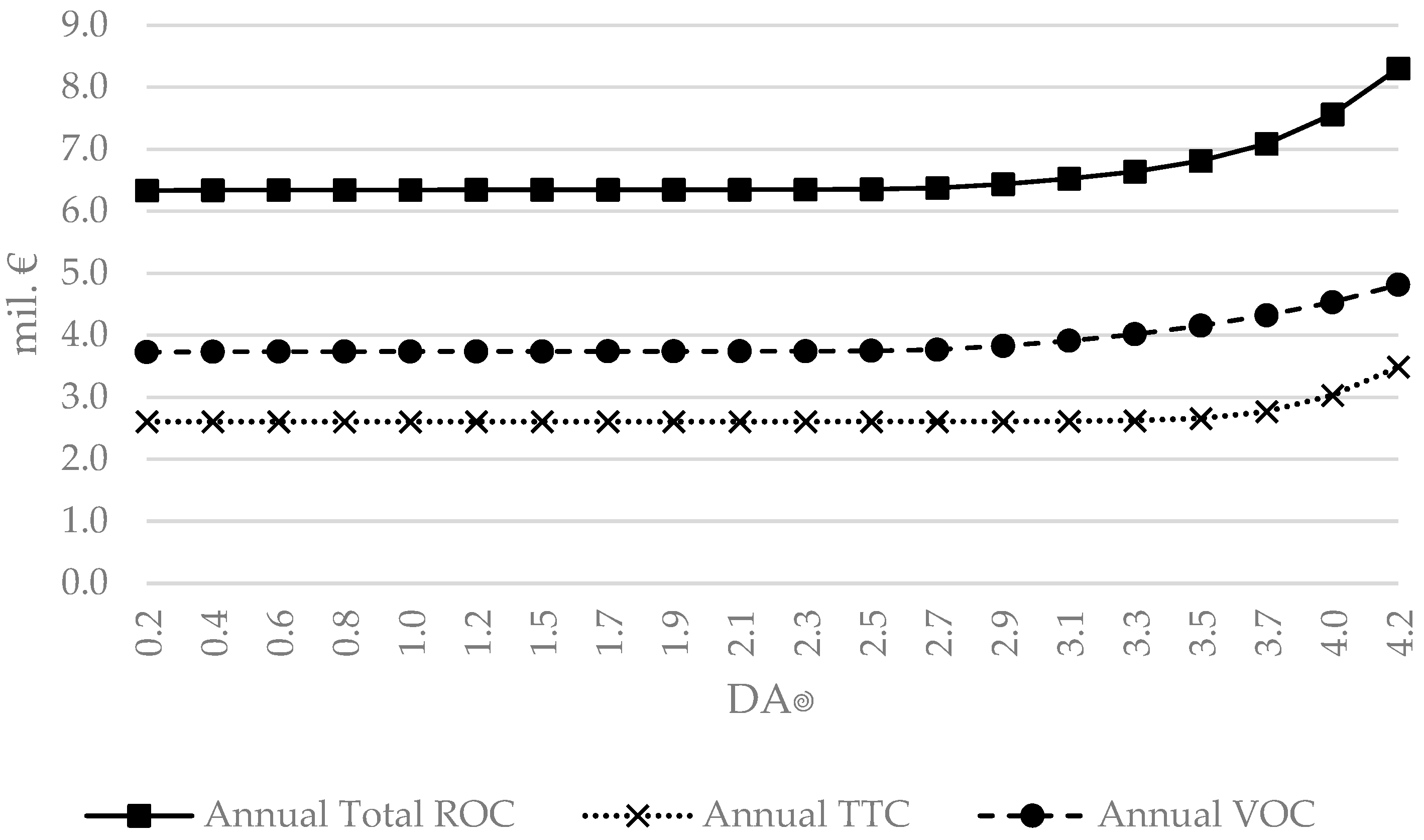
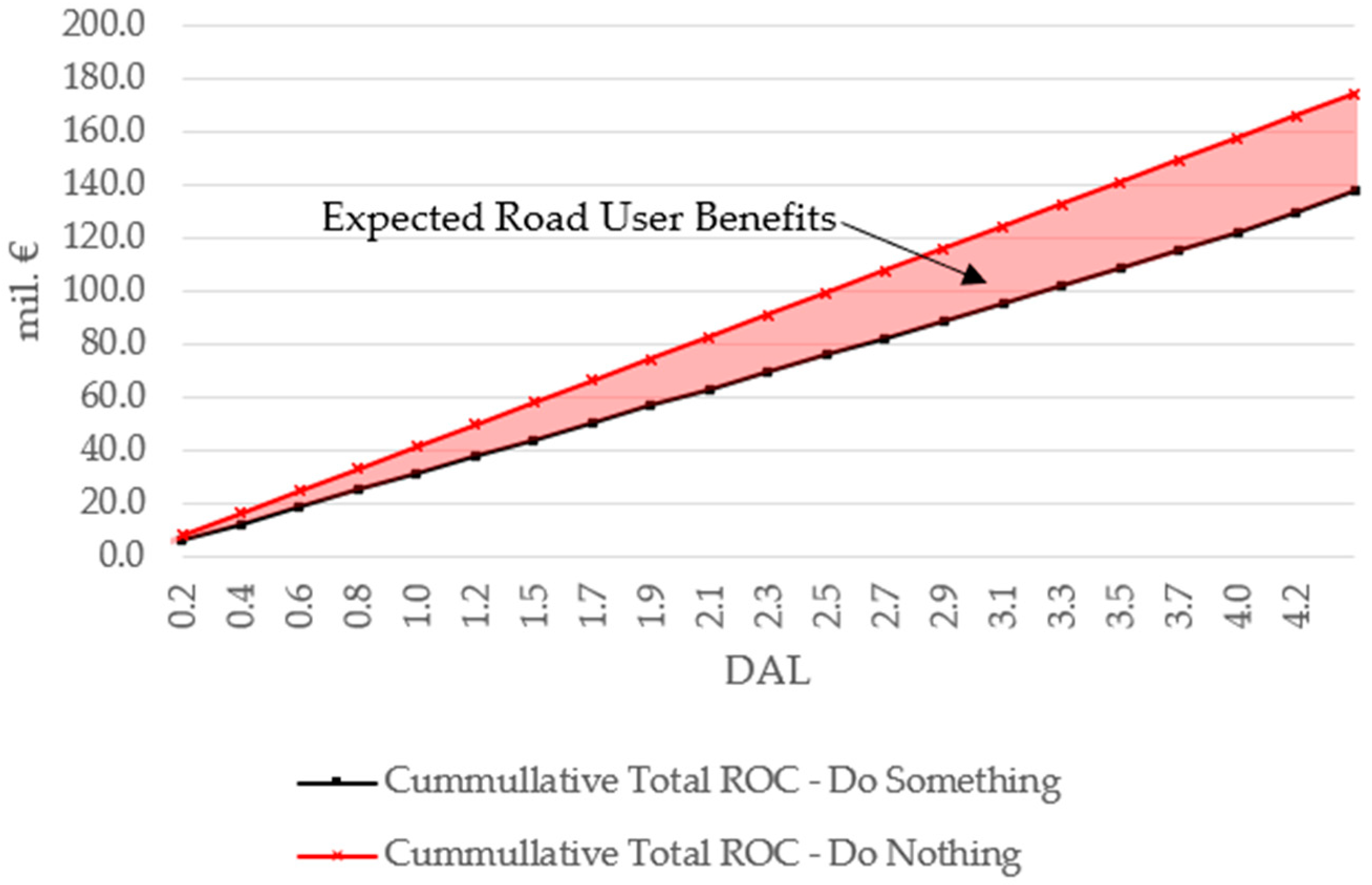
2046	4.812	3.491	8.303	4.812	3.491	8.303	3.129	3.129

and include annual vehicle operating costs (VOC), travel time costs (TTC), total road user costs, and the present value of total road user costs discounted at a rate of 5%. A graphical representation of user costs over the entire pavement life cycle is shown in Figure 10.

The difference between the net road user costs for both scenarios in each year, as defined in Section 4.2 (specifically Equation (6)), generates the expected road user benefits over the entire life cycle, reflecting the progression of pavement deterioration. This relationship is illustrated in Figure 11.

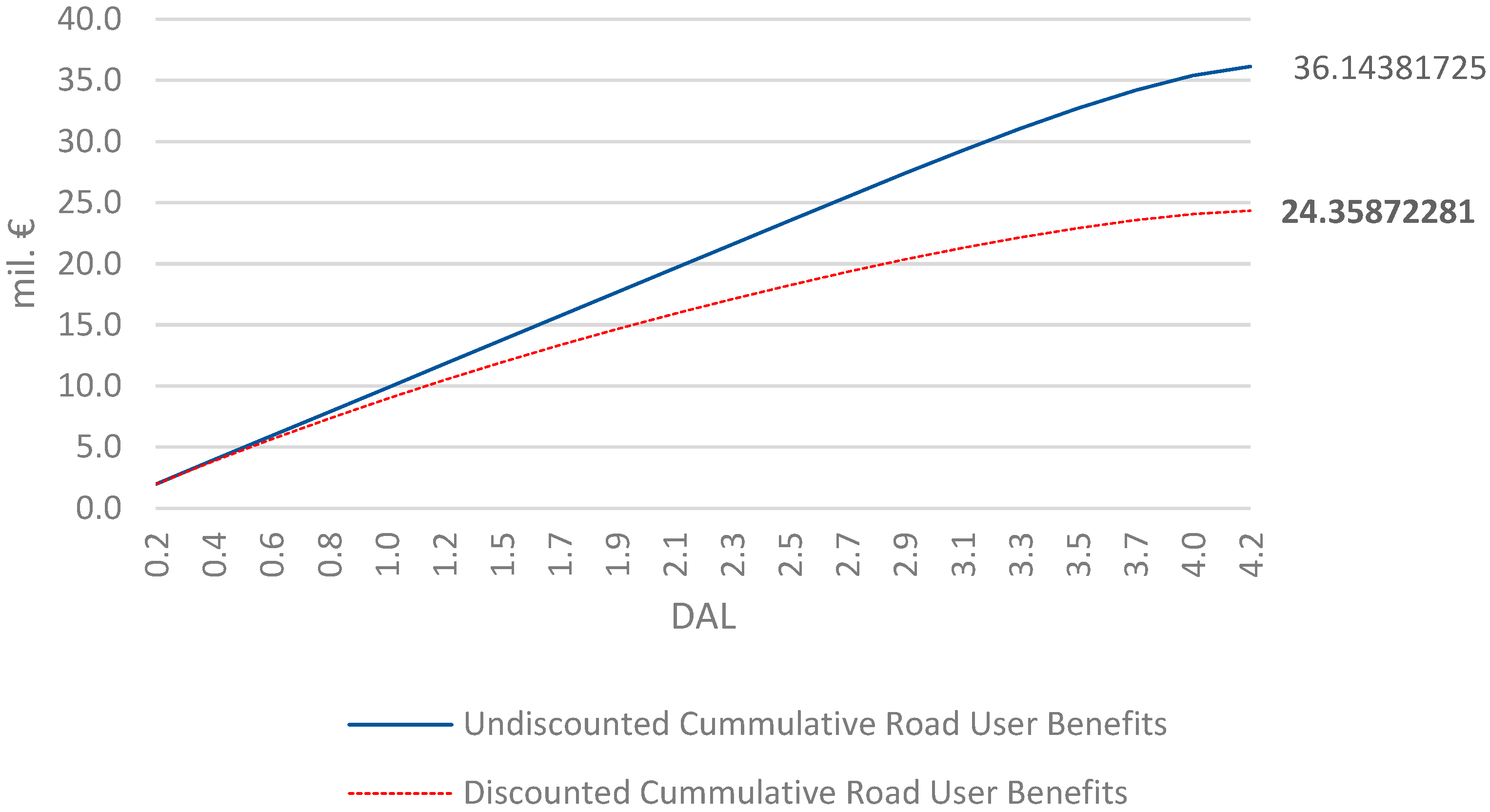
The calculated values of cumulative road user benefits are presented in

Table 9. Cumulative road user benefits, mil. €.

Year	Cumulative Total ROC		Cumulative Road User Benefits	Cumulative Road User Benefits (Discounted)
	Do Something	Do Nothing
2026	6.333	8.303	1.970	1.970
2027	12.669	16.606	3.936	3.843
2028	19.009	24.909	5.900	5.624
2029	25.351	33.212	7.861	7.318
2030	31.694	41.514	9.820	8.930
2031	38.039	49.817	11.779	10.464
2032	44.384	58.120	13.736	11.925
2033	50.730	66.423	15.693	13.315
2034	57.077	74.726	17.649	14.640
2035	63.423	83.029	19.606	15.901
2036	69.771	91.332	21.561	17.101
2037	76.120	99.635	23.515	18.243
2038	82.475	107.938	25.463	19.328
2039	88.848	116.241	27.392	20.351
2040	95.285	124.543	29.259	21.294
2041	101.808	132.846	31.038	22.150
2042	108.448	141.149	32.702	22.912
2043	115.261	149.452	34.191	23.562
2044	122.351	157.755	35.404	24.066
2045	129.914	166.058	36.144	24.359
2046	138.217	174.361	36.144	24.359

. As seen in Figure 12. At the end of the evaluation period, the cumulative road user benefits reach €36,143,817, while the present value of cumulative road user benefits, discounted at a rate of 5%, amounts to €24,358,722. This present value represents the Pavement User Value of the I/14 road after rehabilitation.

6.3. Sensitivity of Road User Benefits to Traffic Intensity and Load-Related Effects

Although the practical application is demonstrated on one road section, the purpose of the case study is primarily to verify the applicability of the proposed road asset valuation framework and to illustrate the interaction between pavement performance, road user costs, and asset value. To examine the robustness of the results under different operating conditions, an additional two-dimensional sensitivity analysis was performed.

The analysis considered changes in two parameters: annual average daily traffic and the equivalent standard axle-load factor. AADT was increased by 10%, 20%, and 30% relative to the base scenario. The Equivalent Standard Axle Load (ESAL) factor was independently increased by 10%, 20%, and 30%, resulting in 15 additional scenarios and 16 combinations including the base scenario. The increase in ESAL represents a higher equivalent damaging effect of the vehicles using the road. In the present analysis, it may also be interpreted as a proxy for a stronger load-induced deterioration response that could be expected for a structurally less robust semi-rigid pavement. Direct uncertainty in the pavement structural parameters is evaluated separately by means of Monte Carlo simulation.

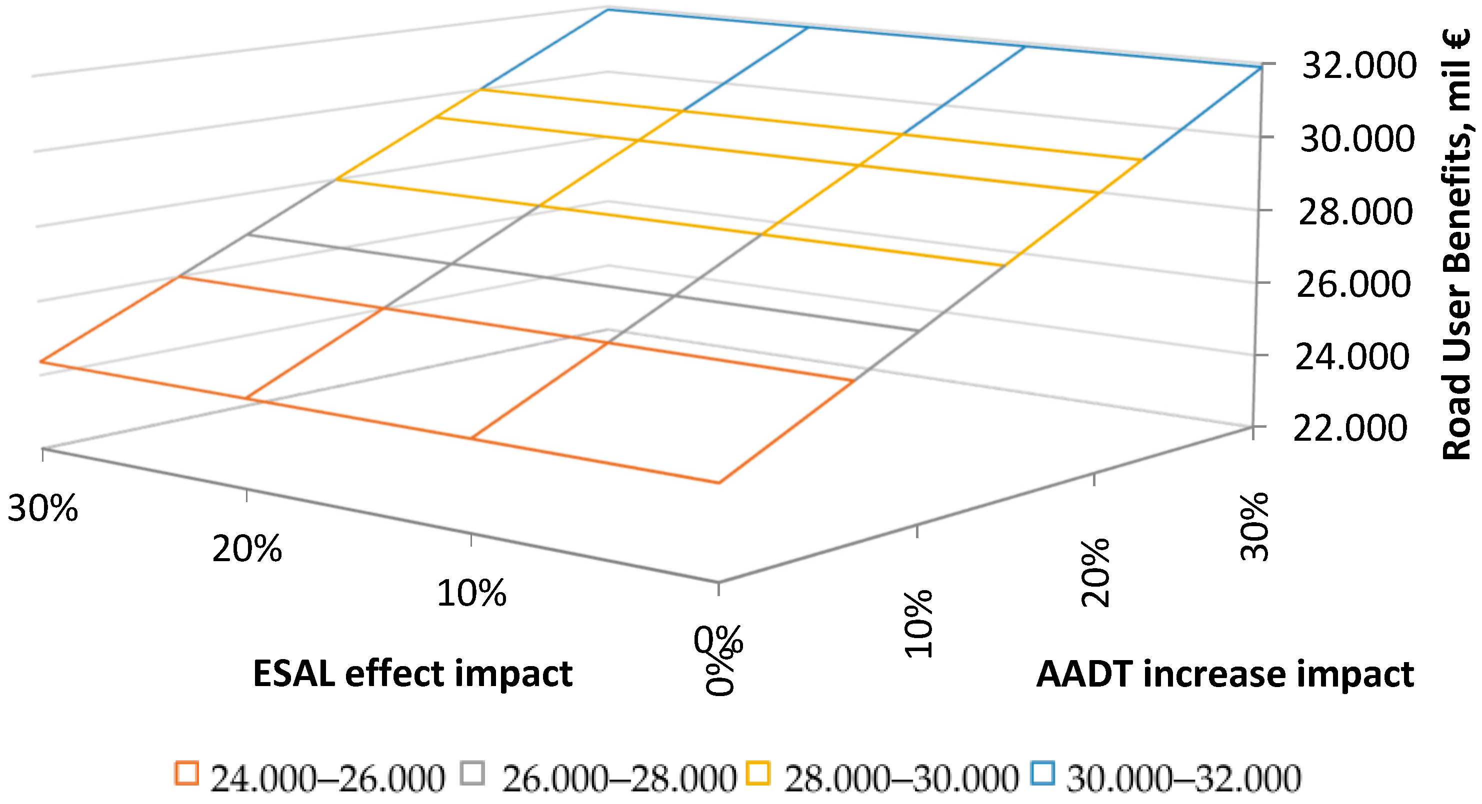
The resulting road user benefits are presented in

Table 10. Road user benefits under combined AADT and ESALF sensitivity scenarios, mil. €.

ESAL increase impact	AADT increase impact
		0%	10%	20%	30%
	0%	24.359	26.844	29.360	31.899
	10%	24.360	26.844	29.361	31.901
	20%	24.360	26.845	29.362	31.902
	30%	24.361	26.846	29.363	31.903

and Figure 13. The results confirm that AADT is the dominant variable. In the base scenario, the calculated road user benefits amount to EUR 24.359 million. Increasing AADT by 10%, 20%, and 30% increases the benefits to approximately EUR 26.844 million, EUR 29.360 million, and EUR 31.899 million, respectively. The 30% increase in AADT therefore produces an increase in road user benefits of approximately 31% compared with the base scenario.

In contrast, increasing ESAL within the investigated interval has only a limited effect on the calculated road user benefits. At the base traffic level, an increase in ESAL of 30% changes the benefits from EUR 24.359 million to EUR 24.361 million. Even for the scenario with a 30% increase in AADT, the corresponding change is only from EUR 31.899 million to EUR 31.903 million.

The relatively low sensitivity to ESAL results from the limit states adopted in the analysis. Pavement performance is assessed from the serviceability perspective using the criterion IRI ≤ 12 m/km and from the structural perspective until the initiation of fatigue cracking at the bottom of the asphalt concrete layers. The analysis therefore does not extend far beyond the fatigue-crack initiation stage. After this limit state, crack propagation could accelerate and develop into wide and interconnected cracking, accompanied by a rapid deterioration of pavement evenness. Such advanced deterioration would substantially increase vehicle operating costs and other road user costs and would probably result in a stronger sensitivity to load-related parameters.

The deterioration relationships used in the case study are representative of the temperate-cool continental conditions of northern Slovakia. The location is characterized by cold winters, freeze–thaw effects, moderate precipitation, and a marked seasonal temperature range. In the HDM-4 climate classification, the site was defined by a semi-arid moisture regime and a temperate-cool temperature regime, with a mean annual temperature of approximately 8 °C and a freeze index of 417 degree-days. Where a country contains several substantially different climatic zones, separate regional calibration of the deterioration relationships would be required. The development and comparison of climate-specific deterioration models are outside the scope of the present study.

6.4. Results

The results of the case study clearly demonstrate the applicability and relevance of the proposed pavement asset value framework based on Full-Life-Cycle deterioration models.

From the structural perspective, the calculated AAP_PC of €8,071,726 represents the value of the pavement asset in its projected condition. When considering the current technical condition of the pavement, characterized by a residual life expectancy of 3 years relative to a projected life of 20 years, the resulting AV_CC is €1,210,759, corresponding to an ISCV of 0.15. This indicates a significantly deteriorated structural condition, confirming the necessity of rehabilitation. After the implementation a complex reconstruction, as opposed to the mill and replace rehabilitation, the AV_CC would increases to €8,554,463 as the complex reconstruction would remedy the 50% reduction in subbase layer value; the ISCV would reach a value of 1.0, representing a fully restored structural condition.

From the user perspective, the HDM-4 analysis highlights the substantial impact of pavement condition on road user costs. The comparison of the “Do Something” and “Do Nothing” scenarios shows that maintaining the pavement in its deteriorated condition leads to persistently high user costs over the entire analysis period. In contrast, the rehabilitation scenario significantly reduces these costs, particularly in the early and middle phases of the life cycle. The cumulative road user benefits over the 20-year evaluation period reach €36,143,817, while their present value, discounted at 5%, amounts to €24,358,722. This value represents the Pavement User Value of the rehabilitated road section and significantly exceeds the structural investment cost, indicating a high economic efficiency of the proposed intervention.

By combining both components, the total pavement asset value after rehabilitation can be expressed as the sum of the Structural Pavement Condition Value €8,071,726 and the Pavement User Value €24,358,722, resulting in a total value of €32,430,449. All these results can be seen in

Table 11. Case study results—total road asset value, €.

Scenario	Investment Costs [€]	Structural Pavement Condition Value		Pavement User Value	Total Road Asset Value Before Rehabilitation	Total Road Asset Value After Rehabilitation
		Value of the Asset in Its Current Technical Condition	Index of Structural Condition Value	Road User Benefits
Do nothing	-	1,210,759	15%	0
Do something	4,867,008	8,071,726	100%	24,358,723	1,210,759	32,430,449

.

This combined valuation provides a quantitative basis for decision-making within cross-asset allocation under constrained financial resources. In cases where the structural condition is critically low (e.g., low ISCV values), priority should be given to structural rehabilitation to prevent loss of load-bearing capacity and potential failure of the asset. Conversely, in situations where structural capacity remains sufficient but surface condition significantly affects user costs, priority should be given to interventions that improve ride quality and reduce user-related costs.

The combined pavement asset value enables the identification of interventions that maximize total benefits by simultaneously considering both structural performance and user-related impacts. This is particularly important in network-level decision-making, where limited resources must be allocated across multiple assets. In such cases, preference should be given to projects with the highest total asset value increase, ensuring the most efficient use of available funding.

Overall, the case study validates the proposed methodology as an effective tool for integrating technical condition assessment with economic evaluation, thereby supporting more informed and efficient decision-making in pavement asset management systems.

6.5. Uncertainty Analysis of Projected Pavement Life and Structural Pavement Condition Value

The deterministic calculation of Structural Pavement Condition Value is based on the ratio between residual life expectancy and projected life expectancy. Although the residual life of the existing pavement can be estimated from diagnostic measurements, the projected life of the rehabilitated pavement is affected by uncertainty in material properties, structural response, and fatigue-model parameters. A Monte Carlo simulation was therefore performed to quantify how this uncertainty propagates through the fatigue–life calculation and subsequently affects the calculated Structural Pavement Condition Value.

6.5.1. Definition of the Material Inadequacy Factor

To represent the combined influence of material-quality uncertainty, a dimensionless material inadequacy factor (MIF) was introduced. The term inadequacy was selected so that positive values represent less favorable material behavior, whereas negative values represent more favorable behavior relative to the reference material. For each Monte Carlo iteration (i), the factor was generated from a bounded standard-normal random variable:

$${\mathrm{M}\mathrm{I}\mathrm{F}}_{\mathrm{i}}=\max \left(-2.5,\min \left(2.5,{\mathsf{\Phi }}^{\left(-1\right)\left({\mathrm{U}}_{\mathrm{i}}\right)}\right)\right)$$

(13)

where

Ui is uniform random variable ${\mathrm{U}}_{\mathrm{i}}~\mathrm{U}\left(\mathrm{0,1}\right)$;

Φ⁻¹ is inverse cumulative distribution function of the standard normal distribution.

The factor was limited to the interval $-2.5\le {\mathrm{M}\mathrm{I}\mathrm{F}}_{\mathrm{i}}\le 2.5$ to prevent the generation of statistically possible but physically implausible combinations of material properties. A value of (MIF = 0) represents the reference material parameters used in the deterministic calculation. Positive values indicate increasing material inadequacy, while negative values indicate material properties that are more favorable than the reference values.

The same MIF value was used to modify all principal fatigue-model inputs within an individual simulation. This approach preserves a physically consistent direction of change among the material parameters. A less adequate material was assumed to exhibit the following:

• A lower fatigue parameter (a);
• A higher fatigue parameter (b);
• A higher calculated radial tensile stress σ_r;
• A lower flexural tensile strength (R).

Conversely, a negative MIF produces a more favorable combination of these parameters. The use of a common latent factor prevents contradictory combinations in which, for example, material strength improves while all other material-related fatigue characteristics simultaneously deteriorate.

The MIF does not represent a directly measurable physical property. It is a stochastic modeling variable introduced to express the combined effect of unobserved variability in material composition, construction quality, and fatigue performance. Its influence is transferred to the individual model parameters through parameter-specific sensitivity coefficients, described in the following subsection.

6.5.2. Stochastic Definition of Fatigue-Model Parameters

The material inadequacy factor was subsequently transferred to the four principal inputs of the fatigue–life model: the fatigue parameters (a) and (b), the radial tensile stress (σ_r), and the flexural tensile strength (R). The deterministic reference values used in the case study were ${\mathrm{a}}_0=0.95,{\mathrm{b}}_0=0.12,{\mathsf{\sigma }}_{\mathrm{r}}=0.43\mathrm{MPa},{\mathrm{R}}_0=2.755\mathrm{MPa}$.

For each Monte Carlo iteration (i), the fatigue parameter (a) was calculated as

$${\mathrm{a}}_{\mathrm{i}}={\mathrm{a}}_{0\left(1-0.05{\mathrm{M}\mathrm{I}\mathrm{F}}_{\mathrm{i}}\right)}$$

(14)

The fatigue parameter (b) was calculated as

$${\mathrm{b}}_{\mathrm{i}}={\mathrm{b}}_{0\left(1+0.02{\mathrm{M}\mathrm{I}\mathrm{F}}_{\mathrm{i}}\right)}$$

(15)

In this case, a positive MIF increases (b). The coefficient 0.02 represents a 2% change in the reference parameter for each unit change in MIF.

The radial tensile stress was calculated as

$${\mathsf{\sigma }}_{\mathrm{r},\mathrm{i}}={\mathsf{\sigma }}_{\left(\mathrm{r},0\right)\left(1+0.02{\mathrm{M}\mathrm{I}\mathrm{F}}_{\mathrm{i}}+0.02{\mathrm{Z}}_{\mathsf{\sigma },\mathrm{i}}\right)}$$

(16)

where Z_σ,i is an independent standard-normal random variable. The first stochastic term represents the systematic influence of material inadequacy, while the second represents additional variability in structural response, including uncertainty associated with loading, layer stiffness, seasonal conditions, and stress calculation:

$${\mathrm{Z}}_{\mathsf{\sigma },\mathrm{i}}~\mathrm{N}\left(\mathrm{0,1}\right)$$

(17)

The flexural tensile strength was calculated as

$${\mathrm{R}}_{\mathrm{i}}={\mathrm{R}}_{0\left(1-0.02{\mathrm{M}\mathrm{I}\mathrm{F}}_{\mathrm{i}}+0.02{\mathrm{Z}}_{\mathrm{R},\mathrm{i}}\right)}$$

(18)

where Z_R,i is another independent standard-normal random variable. A positive MIF reduces the flexural tensile strength, while the independent random term represents residual variability in the measured or estimated material resistance:

$${\mathrm{Z}}_{\mathrm{R},\mathrm{i}}~\mathrm{N}\left(\mathrm{0,1}\right)$$

(19)

The same MIF value was applied to all four parameters within each simulation, thereby introducing a common direction of material-quality change. However, the independent random components assigned to (σ_r) and (R) allowed the model to represent additional variability that cannot be explained solely by the common material inadequacy factor.

A positive MIF simultaneously decreases (a) and (R) and increases (b) and (σ_r). All four changes therefore act in the same direction and reduce the calculated fatigue life. Conversely, a negative MIF produces a more favorable combination of fatigue parameters, structural response, and material resistance.

6.5.3. Monte Carlo Simulation of Fatigue Life

The stochastic values of (a_i), (b_i), (σ_r,i), and (R_i) were subsequently introduced into the fatigue–life relationship. For each Monte Carlo iteration, the logarithm of the allowable number of axle-load repetitions was calculated as

$${\log }_{10}{\mathrm{N}}_{\mathrm{i}}={\displaystyle \frac{{\mathrm{a}}_{\mathrm{i}}{\mathrm{R}}_{\mathrm{i}}-{\mathsf{\sigma }}_{\mathrm{r},\mathrm{i}}}{{\mathrm{b}}_{\mathrm{i}}{\mathrm{R}}_{\mathrm{i}}}}$$

(20)

where N_i is the predicted number of allowable equivalent axle-load repetitions in simulation (i).

The corresponding number of allowable axle-load repetitions was then obtained by inverse logarithmic transformation:

$${\mathrm{N}}_{\mathrm{i}}={10}^{{\log }_{10}{\mathrm{N}}_{\mathrm{i}}}$$

(21)

The projected pavement life expressed in years was calculated by dividing the predicted number of allowable axle-load repetitions by the annual number of equivalent axle loads:

$${\mathrm{P}\mathrm{L}\mathrm{E}}_{\mathrm{i}}={\displaystyle \frac{{\mathrm{N}}_{\mathrm{i}}}{{\mathrm{N}}_{\mathrm{a}\mathrm{n}\mathrm{n}\mathrm{u}\mathrm{a}\mathrm{l}}}}$$

(22)

where N_annual = 208,306 equivalent axle-load repetitions per year for the analyzed road section.

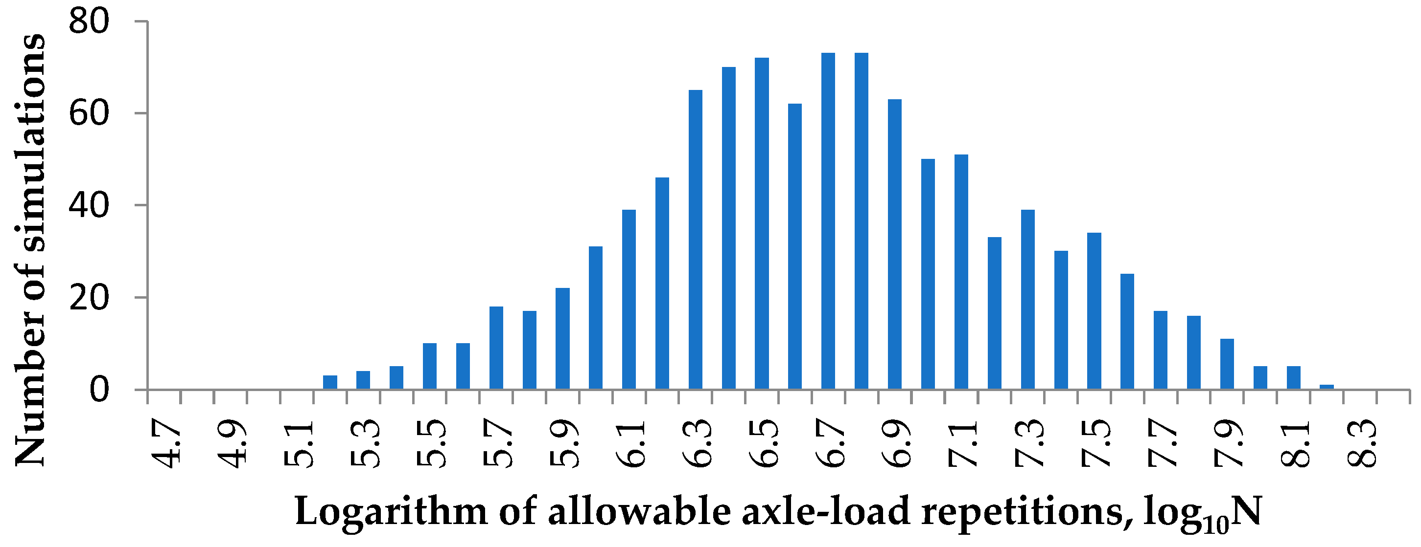
A total of 1000 Monte Carlo iterations were performed, see Figure 14.

The deterministic reference parameters produced

$${\log }_{10}{\mathrm{N}}_0=6.616$$

(23)

corresponding to

$${\mathrm{N}}_0=4.130\times {10}^6$$

(24)

allowable axle-load repetitions and a projected life of approximately 19.82, as was used in the following case study:

$${\mathrm{P}\mathrm{L}\mathrm{E}}_0={\displaystyle \frac{{\mathrm{N}}_0}{{\mathrm{N}}_{\mathrm{a}\mathrm{n}\mathrm{n}\mathrm{u}\mathrm{a}\mathrm{l}}}}=19.82\mathrm{years}$$

(25)

6.5.4. Uncertainty Propagation to Structural Pavement Condition Value

For each Monte Carlo iteration, the simulated projected life expectancy was introduced into the Structural Pavement Condition Value equation:

$${\mathrm{A}\mathrm{V}\mathrm{C}\mathrm{C}}_{\mathrm{i}}=\mathrm{A}\mathrm{A}\mathrm{P}\mathrm{P}\mathrm{C}·\min \left(1,{\displaystyle \frac{\mathrm{R}\mathrm{L}\mathrm{E}}{{\mathrm{P}\mathrm{L}\mathrm{E}}_{\mathrm{i}}}}\right)$$

(26)

The upper limit was introduced to ensure that the calculated current asset value could not exceed the acquisition price of the asset in the projected condition. The case study values were AAPPC = 8,071,726 € and RLE = 3 years.

The resulting AVCC distribution was strongly right-skewed. The principal statistical indicators are presented in

Table 12. Statistical characteristics of the simulated Structural Pavement Condition Value.

Indicator	Result
Deterministic AVCC	€1,210,759
Median	€1,274,483
Mean	€2,139,397
Standard deviation	€2,389,506
Coefficient of variation	108.91%
5th percentile	€104,331
95th percentile	€8,071,726
Simulations deviating by more than ±10%	93%
Simulations deviating by more than ±20%	87%
Simulations deviating by more than ±30%	82%
Simulations reaching the maximum AVCC	9%

.

Although the median remained relatively close to the deterministic estimate, the coefficient of variation exceeded 100%, and 82% of the simulations differed from the deterministic value by more than ±30%. This indicates that uncertainty in projected pavement life is strongly propagated into the calculated asset value. In 9% of simulations, the calculated AVCC reached the upper limit equal to AAPPC.

6.5.5. Evaluation of the Monte Carlo and Statistical Analysis

The Monte Carlo analysis showed that uncertainty in the fatigue-model inputs is substantially amplified by the nonlinear fatigue–life relationship. Although the simulated values of log₁₀N followed an approximately normal distribution, the corresponding distributions of allowable axle-load repetitions, projected pavement life, and Structural Pavement Condition Value were strongly asymmetric.

The deterministic projected life of approximately 20 years was close to the median of the simulated distribution. However, the simulation produced a wide range of projected lives because relatively small changes in the fatigue parameters, material resistance, and calculated tensile stress resulted in multiplicative changes in the number of allowable axle-load repetitions. Very high fatigue–life values should therefore not be interpreted as realistic total pavement service lives. They indicate that bottom–up fatigue cracking would not become the governing failure mechanism within the adopted evaluation horizon.

This uncertainty was directly transferred to the Structural Pavement Condition Value. The simulated median AV_CC remained close to the deterministic estimate, but the coefficient of variation exceeded 100%, and 82% of the simulations differed from the deterministic value by more than ±30%. These results indicate that the asset valuation is highly sensitive to uncertainty in the predicted pavement life, even though the valuation equation itself is deterministic.

In 9% of the simulations, the predicted projected life was equal to or shorter than the assumed residual life. In these cases, the unrestricted valuation equation would produce an AV_CC exceeding the acquisition price of the asset in the projected condition. The calculated value was therefore limited to AA_PPC, which represents the maximum physically and economically meaningful Structural Pavement Condition Value.

The results confirm the importance of reporting uncertainty together with deterministic pavement asset values. A single AV_CC estimate may conceal a wide range of plausible outcomes arising from uncertainty in long-term pavement performance. For practical decision-making, the deterministic value should therefore be supplemented by the median, percentile interval, coefficient of variation, and probability of substantial deviation from the reference estimate.

The presented Monte Carlo analysis evaluates uncertainty associated primarily with the fatigue-based prediction of projected pavement life. It does not include all possible deterioration mechanisms, such as aging, thermal cracking, rutting, environmental degradation, or loss of surface serviceability. Consequently, the calculated uncertainty range should be interpreted as the sensitivity of AV_CC to the selected fatigue–life model and its input parameters rather than as a complete probabilistic prediction of total pavement service life.

7. Conclusions

This paper proposed an integrated framework for evaluating Pavement Asset Condition Value using Full-Life-Cycle deterioration models. The methodology links structural condition, represented by residual service life and Structural Pavement Condition Value, with user-related performance, expressed through road user cost savings and Pavement User Value.

The use of the term Full-Life-Cycle deterioration model in this study refers primarily to the extent of the observational data used for model development rather than to the universal superiority of a particular mathematical function. A model calibrated from partial-life-cycle observations may provide an appropriate representation within the measured range, whereas uncertainty generally increases when the model is extrapolated beyond that range. Full-life-cycle observations reduce the need for such extrapolation by including the initial, intermediate, and terminal stages of pavement performance.

The polynomial form applied in this study was selected because it adequately represented the measured deterioration trajectory, including changes in the rate of deterioration over the investigated life cycle. This selection does not imply that polynomial functions are universally more appropriate than linear, exponential, or mechanistic–empirical models. The most suitable model form should be determined according to the characteristics of the measured data, statistical performance, residual behavior, physical plausibility, and predictive validation. Linear or exponential models may remain appropriate where the observed deterioration trajectory supports their use.

The results confirm that pavement asset value cannot be reliably assessed using only structural indicators or simplified deterioration assumptions. Pavement deterioration affects not only the technical condition of the asset but also vehicle operating costs, travel time costs, and consequently the economic value delivered to road users. Therefore, the integration of structural assessment and user–cost modeling provides a more comprehensive basis for pavement management decision-making.

The case study demonstrated that the proposed rehabilitation strategy substantially increases the Structural Pavement Condition Value and restores the structural index to the projected condition. At the same time, the HDM-4-based comparison of the “Do Something” and “Do Nothing” scenarios showed that improved pavement serviceability generates significant road user benefits over the evaluation period. The total pavement asset value was quantified as the sum of Structural Pavement Condition Value and Pavement User Value, providing a combined metric suitable for project-level and network-level decision-making.

The main scientific contribution of the paper lies in linking Full-Life-Cycle deterioration models, derived from accelerated pavement testing and long-term road monitoring, with economic asset valuation. This approach enables a more realistic estimation of pavement value development over time and supports the identification of rehabilitation interventions that are technically justified and economically efficient.

From a practical engineering perspective, the proposed framework can be applied at both project and network levels to support maintenance and rehabilitation planning under constrained budgets. At the project level, it enables the identification of the optimal intervention timing by simultaneously considering structural deterioration and road user impacts. At the network level, the methodology provides a quantitative basis for prioritizing investments and supporting cross-asset allocation decisions. If the structural condition is critically low, priority should be given to interventions that restore load-bearing capacity and prevent functional failure. If the structural condition is still acceptable but pavement roughness generates high user costs, priority should be given to interventions that improve serviceability and reduce road user costs. In cases where both structural deterioration and user impacts are significant, the combined pavement asset value provides the most appropriate criterion for prioritization.

The study also has several limitations. First, the deterioration models were derived from a limited set of experimental and long-term monitored road sections, and their wider applicability should be verified using additional pavement types, traffic compositions, and rehabilitation technologies. Although the proposed Full-Life-Cycle deterioration models are expected to preserve their general nonlinear shape, their parameters may vary depending on traffic loading, material properties, maintenance strategy, and climatic conditions. The study demonstrates the proposed framework using a single road section under temperate-cool continental climatic conditions. Its transferability was partially examined through 15 additional scenarios combining changes in traffic intensity and equivalent axle-load effects. Nevertheless, further case studies involving different pavement structures, traffic compositions, climatic zones, and regionally calibrated road user–cost models would strengthen the external validation of the framework. Alternative user-cost formulations may change the resulting monetary values, although they are not expected to alter the underlying methodological structure of the proposed asset valuation approach. In practical applications, the methodology may be further refined by classifying long-term pavement performance monitoring (LTPPM) data according to climatic zones and by controlling environmental conditions during Accelerated Pavement Testing (APT). Such climate-specific calibration is particularly relevant for countries characterized by significant climatic variability across their territory. Second, the economic valuation depends on selected cost inputs, discount rate, traffic assumptions, and HDM-4 calibration parameters. Third, the residual value of subbase, subgrade, and embankment layers was estimated using simplified coefficients, which should be further refined through more detailed diagnostic and valuation procedures. Finally, the current framework focuses mainly on structural value and user costs; future research should also incorporate environmental impacts, carbon emissions, safety effects, and uncertainty analysis.

Future work should therefore focus on expanding the database of Full-Life-Cycle deterioration models, improving the calibration of deterioration and road user cost relationships, and developing region-specific models reflecting differences in climate, traffic, and pavement structures. Furthermore, the proposed value-based approach should be integrated into network-level pavement management systems and cross-asset allocation models to support more efficient resource allocation under constrained budgets.