Jerk-Constrained Feedrate Scheduling for Biaxial Contouring Systems: A Planning-to-Execution Simulation Study

Abstract

Biaxial contouring systems are widely used in planar precision motion applications, where the assigned feedrate profile strongly affects motion smoothness, contour-following accuracy, and robustness during servo execution. However, many existing studies mainly focus on either controller-side contour-error regulation or planning-layer time optimality, while the influence of jerk-sensitive feedrate transitions on downstream contouring behavior is still insufficiently examined. To address this issue, this paper proposes a jerk-constrained and execution-aware feedrate scheduling framework for biaxial contouring systems. Starting from the admissible feedrate boundary determined by contour geometry and motion constraints, an acceleration-feasible baseline schedule is first generated through bidirectional reachability propagation. Then, jerk-oriented smoothness refinement and critical-region-preserving correction are introduced to suppress abrupt local transitions while maintaining dynamic admissibility and practical traversal efficiency. The refined path-domain schedule is further reconstructed into time-domain axis-level references for closed-loop contouring evaluation. A planning-to-execution simulation study is conducted on three representative contours, including a rounded triangular contour, an elliptical contour, and a butterfly-cross contour. The proposed method is compared with several baseline scheduling strategies under nominal, low-bandwidth, flexible-resonance, and parameter-mismatch conditions. The simulation results indicate that the proposed scheduler can reduce concentrated jerk responses and resonance-sensitive high-frequency excitation while achieving a more balanced tradeoff among traversal time, contouring accuracy, and robustness. The results also show that the benefit of the proposed method becomes more evident for geometrically complex contours and deteriorated servo conditions. The present study provides simulation-based evidence that execution-aware feedrate scheduling is an effective way to improve biaxial contouring performance without redesigning the low-level servo controller.

1. Introduction

Biaxial contouring systems are widely used in high-speed and high-precision planar motion tasks, such as CNC machining, precision scanning, lithography, and automated manufacturing. Industrial gantry-type platforms constitute a representative application background of this class of systems, while XY stages provide another typical realization. In such tasks, the fundamental requirement is not merely accurate single-axis position tracking but precise contour following with high productivity, acceptable motion smoothness, and strong tolerance to practical actuator and servo limitations.

The importance of multiaxis coordination in contour-following tasks was recognized early through cross-coupled biaxial control [1]. More accurate contour-error estimation methods were subsequently developed to better reflect the true geometric deviation between the commanded contour and the executed trajectory [2]. Task-coordinate-frame formulations, including the global task coordinate frame and the task polar coordinate frame, further improved the representation and regulation of contouring errors in biaxial systems [3,4]. In addition, the evaluation and magnified representation of two-dimensional contouring error was investigated to support more informative geometric performance analysis [5].

Beyond classical cross-coupled contouring control, friction-aware pre-compensation strategies were introduced to reduce both tracking error and contour error under nonlinear motion disturbances [6]. Data-driven prediction and compensation of contour error based on LSTM neural networks were also reported for CNC systems [7]. Model-predictive contouring-error precompensation then provided a more optimization-oriented compensation route for multiaxis motion systems [8]. On the synchronization side, cross-coupled synchronous control based on disturbance-assignment observation and iterative learning control further strengthened the coordination capability of dual-linear-motor servo systems [9]. Newton-ILC-based contouring compensation combined with adaptive jerk control was later proposed to improve repetitive contour-following performance in biaxial motion systems [10].

More recent controller-side studies have continued this direction. Global iterative sliding mode control was developed for industrial biaxial gantry contouring tasks, emphasizing robustness against uncertainties and nonlinear disturbances [11]. A time-varying internal-model-principle-based contour-tracking method further advanced multiaxis contour regulation from a model-based perspective [12]. In parallel, adaptive jerk control on flexure-linked dual-drive gantries highlighted the direct relevance of jerk to vibration-sensitive precision motion [13]. Broader studies on flexure-based nanopositioning stages and iterative learning control for flexible feed drives also indicate that structural flexibility, vibration sensitivity, and high-accuracy repetitive tracking are central issues in precision motion systems [14,15].

In addition to the controller layer, the planning layer also strongly influences traversal efficiency, motion regularity, and the downstream command content imposed on the servo system. Time-optimal contouring control of industrial biaxial gantries showed that properly planned contour traversal can improve both productivity and contouring accuracy [16]. Jerk-limited time-optimal speed planning for arbitrary paths then addressed third-order smoothness more explicitly [17]. Online time-optimal planning with guaranteed feasibility further improved the real-time applicability of constrained multiaxis trajectory generation [18]. Near-time-optimal S-curve scheduling for multiple line segments provided a practical route to smooth and fast velocity generation under axis constraints [19].

Related studies further extended feedrate planning to NURBS tool paths under multiple constraints [20]. Spline-based time-optimal control was also investigated for smooth trajectory generation of CNC machines with geometric constraints [21]. A discrete-time filtering framework with bounded velocity, acceleration, and jerk provided another important route to bounded-derivative motion generation [22]. More recently, adaptive look-ahead smoothing with joint jerk constraints was proposed to reduce stepped feedrate behavior and unstable motion in robot trajectory scheduling [23]. Real-time smooth trajectory generation with velocity-profile blending also demonstrated the value of blending-based smoothness enhancement in complex machining robots [24].

Recent work has pushed this line further by considering simultaneous torque and jerk constraints in near-time-optimal trajectory planning [25]. Comparative studies have also examined the practical performance of jerk-constrained time-optimal planners for industrial manipulators, showing that theoretical optimality alone is not the only relevant criterion in physical execution [26]. Jerk-limited online trajectory scaling has additionally been explored in cable-driven parallel robots, confirming the broader relevance of jerk-aware timing design in constrained motion systems [27]. At the same time, Pareto-based studies have shown that minimum cycle time and motion accuracy are not automatically aligned objectives in industrial feed-drive trajectory planning [28]. Beyond traditional manufacturing systems, contouring-oriented predictive control has even been investigated in time-optimal quadrotor flight, indicating that contouring concepts can be extended to other high-performance motion platforms [29].

Nevertheless, most of the above studies still emphasize either controller-side contour-error regulation or planning-layer feasibility, time optimality, and profile smoothness. Recent biaxial gantry research combining online trajectory planning with contouring control under jerk constraint has moved closer to a joint planner-controller treatment [30]. Recent feedrate-scheduling studies on NURBS interpolation have further emphasized acceleration- and jerk-continuous timing laws, S-shaped feedrate profiles, bidirectional velocity scanning, and round-off-error treatment as important factors for balancing interpolation smoothness, constraint satisfaction, and machining efficiency [31,32]. From the execution-side perspective, iterative contouring-error compensation and data-driven disturbance-observer-based feed-drive compensation also indicate that contouring accuracy is strongly affected by trajectory compensation, axis synchronization, nonlinear friction, disturbance rejection, and feed-drive dynamics [33,34]. However, from the viewpoint of biaxial contouring tasks, there remains insufficient study that treats the feedrate scheduling layer itself as an independent design object and systematically evaluates how it affects motion smoothness, contouring accuracy, resonance-related excitation, and robustness through a complete planning-to-execution simulation chain. While time-optimal planners have laid an important foundation for traversal efficiency, there remains a need to explore scheduling frameworks that explicitly bridge timing-law smoothness with downstream contouring behavior under execution-related constraints.

Motivated by the above observations, this paper develops a jerk-constrained, smoothness-aware, and execution-aware feedrate scheduling framework for biaxial contouring tasks. Rather than redesigning the low-level contouring controller, the present work focuses on the scheduling layer and investigates how the timing law assigned to a prescribed contour affects the final simulated closed-loop execution outcome. Starting from the admissible feedrate boundary determined by contour geometry and motion constraints, an acceleration-feasible baseline schedule is first constructed. On this basis, jerk-oriented smoothness refinement and critical-region-preserving correction are introduced so that the final schedule is not only dynamically admissible but also more suitable for practical biaxial execution. The refined path-domain schedule is then reconstructed into time-domain axis-level position, velocity, acceleration, and jerk references for subsequent contouring evaluation within a unified simulation environment.

The main contributions of this work are summarized as follows. First, a jerk-constrained, smoothness-aware, and execution-aware feedrate scheduling framework is developed for biaxial contouring tasks. The substantive novelty of this framework is not simply the use of a generic S-curve profile, a conventional look-ahead strategy, a time-optimal timing law, or a standard jerk-limited planner. Instead, the proposed method organizes these related concerns from an execution-aware feedrate-scheduling viewpoint by jointly considering admissible-boundary-based baseline generation, jerk-oriented local transition refinement, critical-region preservation, and downstream contouring-performance evaluation. Therefore, the scheduling layer is explicitly linked with the simulated biaxial execution behavior rather than being treated only as an isolated path-domain velocity-generation problem. Unlike existing studies that mainly emphasize either contouring-controller design or planning-layer profile generation alone, the proposed method explicitly treats the feedrate scheduling layer as an independent design object and investigates its downstream influence on contour-following behavior under simulated servo execution. Second, an admissibility-aware and jerk-oriented scheduling mechanism is established. Starting from the admissible feedrate boundary determined by contour geometry and motion constraints, an acceleration-feasible baseline schedule is first constructed through reachability-based propagation. Then, jerk-oriented smoothness refinement and critical-region-preserving correction are introduced to suppress abrupt transition behavior while maintaining dynamic admissibility and practical traversal efficiency. As a result, the generated timing law is not only feasible in the path domain but also more suitable for execution on biaxial servo systems. Third, a complete simulation-based planning-to-execution validation chain is established. Rather than assessing the proposed method only through path-domain feedrate profiles, the resulting schedule is evaluated from the perspectives of feedrate evolution, time-domain kinematics, contouring error, resonance-related excitation, robustness degradation, parameter mismatch, and ablation behavior. This allows the practical merit of the proposed scheduling framework to be examined in terms of motion smoothness, contouring accuracy, and robustness under different path geometries and servo conditions within a unified simulation framework.

The remainder of this paper is organized as follows. Section 2 presents the biaxial contouring system and problem formulation, including the layered contouring task, arc-length parameterization, motion constraints, admissible feedrate boundary, contouring-error metrics, and problem statement. Section 3 develops the proposed jerk-constrained feedrate scheduling method, including acceleration-feasible baseline generation, jerk-oriented smoothness refinement, critical-region-preserving correction, and time-domain reference reconstruction. Section 4 provides simulation results and discussion through a complete planning-to-execution evaluation chain. Finally, Section 5 concludes this paper.

2. Biaxial Contouring System and Problem Formulation

This section establishes the system-level description, geometric representation, motion constraints, and performance definitions used in this study. The research object is a biaxial contouring system for planar precision motion tasks, in which a prescribed contour is executed by two orthogonal servo-driven translational axes. Although the formulation is kept general, a biaxial gantry-based precision contouring platform can be regarded as a representative engineering background because its contouring performance is strongly affected by contour geometry, feedrate evolution, command smoothness, and servo execution quality.

In contour-following tasks, contouring error is generally more representative than independent axis tracking errors, because the final objective is to follow the desired geometric path rather than only to reduce the pointwise tracking deviation of each axis. Therefore, this section formulates the problem from a planning-to-execution viewpoint. The upper planning layer generates a feasible and smooth timing law along a prescribed contour, while the lower execution layer tracks the resulting axis-level references and determines the actual contouring performance. The proposed scheduling method is then developed in Section 3.

2.1. System Overview and Layered Contouring Task

Consider a planar contour described by the arc-length parameter s, which is written as

$$\mathbf{P}(s)=\left[\begin{array}{c}{P}_x\left(s\right)\\ P_y\left(s\right)\end{array}\right], s\in [0,L],$$

(1)

where $s$ is the arc-length parameter and $L$ is the total contour length. The actual closed-loop position of the biaxial system is denoted by $\mathit{q}\left(t\right)=\left[x\right(t), y\left(t\right){]}^{\mathrm{T}}$, where $x\left(t\right)$ and $y\left(t\right)$ are the executed positions of the two orthogonal axes.

The reference trajectory sent to the execution layer is generated by assigning a timing law s(t) to the prescribed contour:

$${\mathit{q}}_{\mathrm{r}}(t)=\mathit{P}(s(t\left)\right),$$

(2)

where $s\left(t\right)$ is the timing law assigned to the prescribed contour. The feedrate, tangential acceleration, and scalar feedrate jerk are denoted by $v\left(t\right)=\dot{s}\left(\mathrm{t}\right)$, $\mathrm{a}\left(\mathrm{t}\right)=\ddot{s}\left(\mathrm{t}\right)$, and $\mathrm{j}\left(\mathrm{t}\right)=\stackrel{\mathrm{⃛}}{s}\left(\mathrm{t}\right)$, respectively.

From a system viewpoint, the contouring process can be divided into four layers: the path geometry layer, the feedrate scheduling layer, the reference generation layer, and the biaxial servo execution layer. The path geometry layer provides the prescribed contour and its local geometric features. The scheduling layer determines the timing law under motion constraints. The reference generation layer converts the path-domain motion into axis-level commands. Finally, the servo execution layer determines the actual contouring accuracy. In this work, the main design focus is the scheduling layer, while the effectiveness of the generated trajectory is evaluated through the simulated closed-loop behavior of the biaxial system.

2.2. Arc-Length Parameterization and Path-to-Axis Kinematic Mapping

For the arc-length-parameterized contour, the local tangent-normal frame is introduced to describe the contour geometry. The unit tangent vector, unit normal vector, and curvature are defined as

$$\mathit{t}(s)={\displaystyle \frac{\mathrm{d}\mathit{P}\left(s\right)}{\mathrm{d}s}},\mathit{n}(s)={\mathit{R}}_{{\displaystyle \frac{\mathbf{\pi }}{\mathbf{2}}}}\mathit{t}(s),\kappa (s)=∥{\displaystyle \frac{\mathrm{d}\mathit{t}\left(s\right)}{\mathrm{d}s}}∥$$

(3)

where $\mathit{t}\left(s\right)$, $\mathit{n}\left(s\right)$, and $\kappa \left(s\right)$ are the unit tangent vector, unit normal vector, and curvature, respectively, and ${\mathit{R}}_{{\displaystyle \frac{\mathbf{\pi }}{\mathbf{2}}}}$ denotes a rotation of $90°$. The tangent-normal frame is used because contouring error is naturally defined with respect to the local geometry of the desired contour.

Based on (2), the first-order mapping from path-domain motion to axis-level reference velocity is

$${\dot{\mathit{q}}}_{\mathrm{r}}(t)=\mathit{t}(s)v(t).$$

(4)

The second-order mapping from path-domain motion to axis-level reference acceleration is

$${\ddot{\mathit{q}}}_{\mathrm{r}}(t)=\mathit{t}(s)a(t)+\kappa (s)\mathit{n}(s)v^2(t).$$

(5)

Equation (5) shows that the reference acceleration consists of a tangential component caused by feedrate variation and a normal component caused by contour curvature. Therefore, even if the scalar timing law is smooth, highly curved contour segments may still lead to large acceleration demand.

The corresponding third-order mapping can be written as

$${\stackrel{\mathbf{⃛}}{\mathit{q}}}_{\mathrm{r}}(t)={\mathit{P}}^{\prime }\left(s\right)j(t)+3{\mathit{P}}^{″}\left(s\right)v\left(t\right)a(t)+{\mathit{P}}^{‴}\left(s\right)v^3\left(t\right).$$

(6)

This expression is retained because it directly explains why jerk-constrained scheduling is important. The axis-level high-order reference content depends not only on the scalar jerk $j\left(t\right)$ but also on contour geometry and the coupling among $v\left(t\right)$, $a\left(t\right)$, and the spatial derivatives of $\mathit{P}\left(s\right)$. Therefore, suppressing abrupt feedrate transitions can reduce high-frequency command excitation and improve the subsequent servo contouring behavior.

2.3. Motion Constraints and Admissible Feedrate Boundary

In a practical biaxial contouring system, motion feasibility is limited by actuator capability and contour geometry. The axis-level velocity, acceleration, and jerk limits can be expressed in compact vector form as

$$\left|\dot{{\mathit{q}}_{\mathbf{r}}}\left(t\right)\right|⪯{\mathit{V}}_{\max },\left|\ddot{{\mathit{q}}_{\mathbf{r}}}\left(t\right)\right|⪯{\mathit{A}}_{\max },\left|{\stackrel{⃛}{\mathit{q}}}_{\mathbf{r}}\left(t\right)\right|⪯{\mathit{J}}_{\max },$$

(7)

where $⪯$ denotes componentwise inequality. These axis-level constraints are ultimately related to the path-domain timing law through the kinematic mappings in (4)–(6).

For feedrate scheduling, the dominant path-domain constraints are written as

$$0\le v\left(t\right)\le V_{\max },\left|a\left(t\right)\right|\le A_{\tan ,\max },\left|j\left(\mathrm{t}\right)\right|\le J_{\max }.$$

(8)

Here, $V_{\max }$, $A_{\tan ,\max }$, and $J_{\max }$ denote the allowable feedrate, tangential acceleration, and scalar feedrate jerk, respectively. Similar constrained timing-law formulations are commonly used in contouring-oriented trajectory planning.

In addition to these direct motion limits, contour geometry imposes a curvature-related normal acceleration constraint. According to (5), the normal acceleration component should satisfy

$$\left|\kappa \left(s\right)\right|v^2\left(s\right)\le A_{\mathrm{n},\max },$$

(9)

where $A_{\mathrm{n},\max }$ is the allowable normal acceleration. Accordingly, the curvature-induced admissible speed boundary is obtained as

$$V_{\mathrm{curve}}(s)=\sqrt{{\displaystyle \frac{A_{\mathrm{n},\max }}{\left|\kappa \left(s\right)\right|+{\epsilon }_{\kappa }}}},$$

(10)

where ${\epsilon }_{\kappa }>0$ is a small regularization constant used to avoid numerical singularity in near-zero-curvature regions.

The axis-level velocity limits can also be reflected in the path domain through

$$V_{\mathrm{xy}}(s)=\min \left({\displaystyle \frac{V_{x,\max }}{\left|P_x^{\prime }\left(s\right)\right|+{\epsilon }_v}},{\displaystyle \frac{V_{y,\max }}{\left|P_y^{\prime }\left(s\right)\right|+{\epsilon }_v}}\right),$$

(11)

where $V_{\mathrm{xy}}\left(s\right)$ denotes the path-domain speed bound induced by the two axis-velocity limits. The small positive constant ${\epsilon }_v$ is explicitly included in the denominators to avoid numerical division by zero when $\left|P_x^{\prime }\left(s\right)\right|$ or $\left|P_y^{\prime }\left(s\right)\right|$ approaches zero. Its value is selected to be sufficiently small, so that the regularization improves numerical robustness without changing the physical meaning of the axis-velocity constraint.

Combining the global feedrate limit, the curvature-induced speed limit, and the axis-velocity-induced speed limit, the admissible feedrate boundary is defined as

$$V_{\mathrm{FLC}}(s)=\min \left(V_{\max },V_{\mathrm{curve}}(s),V_{\mathrm{xy}}(s)\right).$$

(12)

For clarity, the symbols used in the admissible feedrate boundary are further defined here. $V_{\max }$ denotes the prescribed global upper bound of the scalar feedrate. $V_{x,\max }$ and $V_{y,\max }$ denote the maximum allowable axis velocities of the $x$- and $y$-axes, respectively. $V_{\mathrm{curve}}\left(s\right)$ denotes the curvature-induced path-domain speed limit obtained from the normal-acceleration constraint. $V_{\mathrm{xy}}\left(s\right)$ denotes the path-domain speed limit induced by the two axis-velocity constraints. $V_{\mathrm{FLC}}\left(s\right)$ denotes the final admissible feedrate boundary used by the scheduler after combining the global feedrate limit, the curvature-induced speed limit, and the axis-velocity-induced speed limit. The parameter ${\epsilon }_v$ is a small positive regularization constant introduced to avoid numerical division by zero when the tangent component of an axis is close to zero. In the scheduling stage, $v$ or $v\left(s\right)$ denotes the scalar feedrate profile assigned along the arc-length coordinate $s$.

A feasible feedrate profile must then satisfy

$$0\le v\left(s\right)\le V_{\mathrm{FLC}}(s),\forall s\in [0, L].$$

(13)

This boundary transforms the contour geometry and axis capability into a path-dependent speed ceiling. Regions with large curvature or strong axis-level restrictions naturally force lower admissible speed and become geometric bottlenecks.

For later analysis, the bottleneck point and the critical region are defined as

$$s_{\mathrm{b}}=\arg \underset{\mathrm{s}\in [0,L]}{\min }{V}_{\mathrm{FLC}}(s),{ \Omega }_{\mathrm{crit}}=\{s\in [0, L]\mid V_{\mathrm{FLC}}(s)\le {\eta }_v{V}_{\max }\}, 0<{\eta }_v<1.$$

(14)

Here, $s_{\mathrm{b}}$ denotes the most restrictive point along the contour, while ${\Omega }_{\mathrm{c}\mathrm{r}\mathrm{i}\mathrm{t}}$ denotes the set of path segments where the admissible feedrate is significantly reduced. The parameter ${\eta }_v$ is a dimensionless threshold coefficient satisfying 0 < ${\eta }_v$ < 1, and it determines how close the admissible feedrate boundary must be to its global upper bound before a path segment is identified as a critical region. A smaller ${\eta }_v$ selects only more restrictive segments, whereas a larger ${\eta }_v$ includes a wider neighborhood around speed-limited regions. These definitions are useful for interpreting the local speed reduction and the later critical-region-preserving refinement.

2.4. Contouring Error Metrics and Traversal Time Evaluation

In contour-following applications, contour error and axis tracking error are not equivalent. The contouring error measures the deviation normal to the desired contour and is therefore more directly related to spatial contouring quality. Let the Cartesian tracking deviation relative to the scheduled reference point be

$${\mathit{e}}_{\mathrm{xy}}(t)=\mathit{q}\left(t\right)-\mathit{P}(s(t)),$$

(15)

where $\mathit{q}\left(t\right)$ is the actual closed-loop position and $\mathit{P}\left(s\right(t\left)\right)$ is the scheduled reference contour point.

Using the local tangent-normal frame, the tangential error and contouring error are defined as

$$e_{\mathrm{t}}(t)={\mathit{t}}^{\mathrm{T}}(s(t)){\mathit{e}}_{\mathrm{xy}}(t), e_{\mathrm{c}}(t)={\mathit{n}}^{\mathrm{T}}(s(t)){\mathit{e}}_{\mathrm{xy}}(t).$$

(16)

The tangential error $e_{\mathrm{t}}\left(t\right)$ describes the deviation along the direction of contour progression and is related to lag or advancement, while the contouring error $e_{\mathrm{c}}\left(t\right)$ describes the normal deviation from the desired contour. For contours containing self-intersection or near-self-intersection regions, the tangent-normal frame is selected according to the continuous evolution of $s\left(t\right)$, so that artificial branch switching is avoided.

The overall geometric deviation is defined as

$$e_{\mathrm{geom}}(t)={‖{\mathit{e}}_{\mathrm{xy}}\left(t\right)‖}_2.$$

(17)

For global performance evaluation over the full execution interval $\left[0,T\right]$, the main contouring and geometric error indices are defined as

$$e_{\mathrm{c}, \mathrm{rms}}=\sqrt{{\displaystyle \frac{1}{T}}{\int }_0^T{e}_{\mathrm{c}}^2(t)\mathrm{d}t},e_{\mathrm{geom},\mathrm{rms}}=\sqrt{{\displaystyle \frac{1}{T}}{\int }_0^T{e}_{\mathrm{geom}}^2(t)\mathrm{d}t}.$$

(18)

The corresponding peak error indices are defined as

$$e_{\mathrm{c},\max }=\underset{\mathrm{t}\in [0,T]}{\max }\left|e_{\mathrm{c}}\left(t\right)\right|,e_{\mathrm{geom},\max }=\underset{t\in [0,T]}{\max }{e}_{\mathrm{geom}}(t).$$

(19)

The smoothness-related jerk indices are defined as

$$j_{\mathrm{rms}}=\sqrt{{\displaystyle \frac{1}{T}}{\int }_0^T{j}^2(t)\mathrm{d}t},j_{\mathrm{peak}}=\underset{t\in [0,T]}{\max }\left|j\left(t\right)\right|.$$

(20)

These indices are sufficient for the evaluation in this study because the objective is not only to shorten the traversal time but also to reduce abrupt kinematic transitions and improve contouring performance after servo execution.

For a feasible feedrate profile $v\left(s\right)$, the total traversal time is computed as

$$T={\int }_0^L{\displaystyle \frac{1}{v\left(s\right)}}\mathrm{d}s.$$

(21)

In numerical implementation, $T$ can be approximated by the trapezoidal summation of adjacent path samples. Equation (21) shows the basic tradeoff in feedrate planning: increasing $v\left(s\right)$ can reduce traversal time, but an excessively aggressive schedule may increase acceleration and jerk burden, introduce high-frequency command content, and degrade contouring accuracy after servo execution. Therefore, time efficiency, motion smoothness, and contouring accuracy should be evaluated jointly.

2.5. Problem Statement

Based on the above formulation, the planning task considered in this paper is to determine a feasible timing law s(t) for a prescribed contour $\mathit{P}$(s), such that the generated reference trajectory satisfies the admissible motion constraints, maintains acceptable traversal efficiency, avoids unnecessary jerk concentration, and leads to improved contouring performance after biaxial servo execution.

This problem is not treated as a purely minimum-time trajectory generation problem. A timing law that only pursues aggressive traversal may produce large jerk peaks, stronger high-frequency reference excitation, and degraded contouring behavior in the execution layer. Therefore, the objective of this study is more appropriately regarded as a smoothness-aware and execution-aware feedrate scheduling problem, where efficiency, motion regularity, and contouring quality are balanced in an integrated manner [2].

Accordingly, the output of the planning layer is a dynamically admissible and smooth reference evolution along the prescribed contour. The merit of the generated schedule is ultimately assessed by its influence on traversal time, jerk behavior, contouring accuracy, and robustness under different servo execution conditions. On this basis, Section 3 develops the proposed jerk-constrained feedrate scheduling framework.

3. Jerk-Constrained Feedrate Scheduling Method

This section develops the jerk-constrained feedrate scheduling method for the biaxial contouring problem formulated in Section 2. The purpose of the proposed method is not to redesign the low-level servo controller but to generate a dynamically admissible and execution-friendly reference trajectory for the downstream biaxial system. Compared with a purely minimum-time scheduling strategy, the proposed method emphasizes the balance among traversal efficiency, motion smoothness, and contouring performance after servo execution.

The method is organized into four main stages. First, an admissible feedrate boundary is obtained from the geometric and motion constraints defined in Section 2. Second, an acceleration-feasible baseline schedule is generated through bidirectional propagation under this boundary. Third, a jerk-oriented refinement is introduced to suppress abrupt local transitions in the feedrate profile. Finally, the refined path-domain schedule is reconstructed into time-domain axis-level reference commands for closed-loop contouring evaluation.

3.1. Design Objective and Method Overview

According to the problem statement in Section 2.5, the desired output of the planning layer is a timing law $s\left(t\right)$ that satisfies the admissible feedrate boundary, acceleration constraint, and jerk-related smoothness requirement. In an ideal form, the scheduling tendency can be expressed as a balance among traversal time, jerk-related smoothness, and execution-related excitation:

$$\underset{s\left(\mathrm{t}\right)}{\min }\Phi =T+{\lambda }_j{J}_s+{\lambda }_e{\Psi }_{\mathrm{exe}},$$

(22)

where $T$ is the total traversal time, $J_s$ is a jerk-related smoothness penalty, ${\Psi }_{\mathrm{exe}}$ denotes an execution-related penalty, and ${\lambda }_j$ and ${\lambda }_e$ are weighting coefficients.

Equation (22) is used only to clarify the design tendency of the proposed scheduler. This study does not claim to solve a full nonlinear optimal-control problem to global optimality. Instead, the proposed method is an engineering-oriented scheduling framework that constructs a feasible baseline feedrate and then improves its smoothness while preserving the major restrictive regions of the admissible boundary.

From the viewpoint of optimality, the staged procedure should be interpreted as a structured approximation to the design tendency in Equation (22) rather than as an exact global optimizer. Since traversal time, jerk-related smoothness, execution-related excitation, and path-dependent constraints are coupled in a nonlinear manner, solving the complete problem to global optimality would lead to a substantially more complicated optimal-control problem. The proposed method therefore does not guarantee the globally minimum value of the objective function in Equation (22), nor does it claim to produce a strictly time-optimal feedrate schedule.

However, this approximation is designed to avoid the loss of discrete feasibility in the scheduling process. The acceleration-feasible baseline generated by bidirectional propagation provides an initial profile that satisfies the admissible feedrate boundary and the tangential-acceleration reachability condition at the path samples. During the subsequent smoothing process, a candidate profile may become smoother but may also temporarily violate local feasibility. For this reason, the admissibility correction in Equation (32) is applied after each smoothing stage. This correction projects the candidate profile back to the discrete feasible range defined by the feedrate boundary and the tangential-acceleration constraint in Equation (30). Therefore, the main theoretical consequence of the staged approximation is a possible loss of strict global optimality rather than a loss of the discrete feedrate-boundary and acceleration feasibility required for execution.

The complete scheduling process can be summarized as follows. The input of the method includes the prescribed contour $\mathit{P}\left(s\right)$, the admissible feedrate boundary $V_{\mathrm{FLC}}\left(s\right)$, and the motion constraints. The output is a refined feedrate profile $v^{\star }\left(s\right)$, together with the reconstructed timing law $s\left(t\right)$ and the corresponding axis-level reference commands. This input-processing-output structure makes the method suitable for simulation-based validation and later implementation on biaxial gantry-based contouring platforms.

3.2. Acceleration-Feasible Baseline Feedrate Generation

Let the prescribed contour be discretized into $N$ path samples. The $i$-th path point is denoted by $s_i$, and the interval between adjacent samples is

$$\Delta s_{\mathrm{i}}=s_{\mathrm{i}}-s_{\mathrm{i}-1},i=2,3,\dots ,N.$$

(23)

The corresponding admissible feedrate boundary is written as

$$V_i=V_{\mathrm{FLC}}(s_i),i=1,2,\dots ,N.$$

(24)

The boundary $V_i$ gives the maximum allowable feedrate at each path point. However, a pointwise speed boundary does not guarantee that two adjacent path points can be connected under the tangential acceleration limit. Therefore, bidirectional propagation is used to construct an acceleration-feasible baseline schedule.

Starting from the initial condition $v_1^{\mathrm{f}}=0$, the forward propagation is given by

$$v_i^{\mathrm{f}}=\min \left(V_i,\sqrt{{\left(v_{i-1}^{\mathrm{f}}\right)}^2+2A_{\tan ,\max }\Delta s_i}\right),i=2,3,\dots ,N.$$

(25)

This forward pass suppresses infeasible feedrate growth from upstream path samples. To ensure sufficient deceleration capability for downstream restrictive regions and the terminal condition, a backward propagation is then performed as

$$v_i^{\mathrm{b}}=\min \left(v_i^{\mathrm{f}},\sqrt{{\left(v_{i+1}^{\mathrm{b}}\right)}^2+2A_{\tan ,\max }\Delta s_{i+1}}\right),\mathrm{i}=N-1,N-2,\dots ,1,$$

(26)

with $v_N^{\mathrm{b}}=0$. The acceleration-feasible baseline schedule is then defined as

$$v_i^{\left(0\right)}=v_i^{\mathbf{b}},i=1,2,\dots ,N.$$

(27)

The physical meaning of (25)–(27) is straightforward. The admissible boundary $V_i$ specifies the local speed ceiling, while the bidirectional propagation determines a globally reachable speed profile below this ceiling. Therefore, $v_i^{\left(0\right)}$ provides a geometry-consistent and acceleration-feasible baseline for the subsequent jerk-oriented refinement.

To examine the time-domain implication of the baseline schedule, the local time increment is approximated by

$$\Delta t_i={\displaystyle \frac{2\Delta s_i}{v_{i-1}^{\left(0\right)}+v_i^{\left(0\right)}+{\epsilon }_v}},i=2,3,\dots ,N,$$

(28)

where ${\mathrm{\epsilon }}_{\mathrm{v}}$ is a small positive constant used to avoid numerical singularity. The local acceleration and jerk can then be estimated from the discrete speed profile. Although the baseline schedule is acceleration-feasible by construction, it may still contain sharp local transitions near restrictive path regions. These transitions can generate large jerk peaks after time-domain reconstruction, which motivates the smoothness refinement stage.

3.3. Jerk-Oriented Smoothness Refinement

Acceleration feasibility does not automatically guarantee execution-friendly motion. In a biaxial contouring system, the path-domain feedrate profile is converted into axis-level position, velocity, acceleration, and jerk references. Therefore, local switching-like variations in the feedrate profile may be amplified into high-order command components, especially near bottleneck regions or rapidly changing curvature segments.

To reduce such undesirable behavior, the baseline schedule is refined by a jerk-oriented smoothing mechanism. The refinement tendency can be described by the following regularized form:

$$\underset{\mathit{v}}{\min }{‖\mathit{v}\text{-}‖}_2^2+{\lambda }_1{‖{\mathit{D}}_1\mathit{v}‖}_2^2+{\lambda }_2{‖{\mathit{D}}_2\mathit{v}‖}_2^2,$$

(29)

subject to

$$0\le v_i\le V_i,\left|{\displaystyle \frac{v_i^2-v_{i-1}^2}{2\Delta s_i}}\right|\le A_{\tan ,\max }.$$

(30)

Here, $\mathit{v}=[v_1,v_2,\dots ,v_N{]}^{\mathrm{T}}$, ${\mathit{D}}_1$ and ${\mathit{D}}_2$ denote the first- and second-order difference operators, respectively, and ${\lambda }_1$ and ${\lambda }_2$ are weighting coefficients. The first term in (29) preserves the main shape of the acceleration-feasible baseline. The second and third terms penalize abrupt slope changes and local curvature variations in the discrete feedrate profile, which are closely related to jerk amplification after reconstruction.

In practical implementation, the regularized idea is realized by a multi-stage smoothing process with admissibility correction. Let ${\mathit{v}}^{\left(k\right)}$ denote the schedule after the $k$-th refinement stage. A candidate smoothed profile is first computed as

$${\tilde{\mathit{v}}}^{\left(k\right)}=(1-{\alpha }_k){\mathit{v}}^{(k-1)}+{\alpha }_{k}S\left({\mathit{v}}^{(k-1)}\right),$$

(31)

where $S(\cdot )$ is a local smoothing operator and ${\alpha }_k\in (0, 1)$ is the blending factor. After smoothing, the candidate profile is projected back to the admissible range:

$${\mathit{v}}^{\left(k\right)}={\Pi }_{\mathit{A}}\left({\tilde{\mathit{v}}}^{\left(k\right)}\right),$$

(32)

where ${\Pi }_A(\cdot )$ denotes the correction operation that enforces the feedrate boundary and acceleration feasibility conditions in (30).

Compared with a single aggressive smoothing operation, the multi-stage refinement in (31) and (32) gradually attenuates local switching tendencies while maintaining compatibility with the admissible boundary. Therefore, the refined profile is not merely smoother in appearance but remains dynamically executable for the biaxial system.

The feasibility-preserving role of Equation (32) can be further clarified as follows. The smoothing operator in Equation (31) is used only to generate a candidate feedrate profile, whereas the accepted profile at each refinement stage is always the corrected result after admissibility projection. Consequently, even if the smoothing operation locally increases the feedrate above the admissible boundary or produces an acceleration-infeasible transition between adjacent path samples, the correction step re-enforces the constraints before the next refinement stage starts. In the numerical implementation, a final forward–backward correction pass is also applied after the last smoothing stage to remove possible small violations caused by discretization and interpolation. Thus, the proposed refinement is heuristic with respect to global optimality but constraint-aware with respect to the discrete feedrate-boundary and tangential-acceleration feasibility.

The weighting coefficients, smoothing-stage number, and blending factors are selected according to their functional roles in the refinement process. The coefficient ${\lambda }_1$ controls the penalty on the first-order variation of the discrete feedrate profile and mainly affects the local slope change of the scheduled feedrate. A larger ${\lambda }_1$ generally produces a more gradual feedrate transition but may also increase traversal time because the profile becomes less aggressive near restrictive regions. The coefficient ${\lambda }_2$ controls the penalty on the second-order variation of the feedrate profile and is more closely related to the suppression of local oscillatory or switching-like behavior. Increasing ${\lambda }_2$ can reduce jerk-sensitive fluctuations, but an excessively large value may over-smooth the profile and weaken the response to short geometric bottlenecks.

The number of smoothing stages $K$ and the blending factor αk determine how strongly the baseline profile is modified during the multi-stage refinement. A small $K$ or a small ${\alpha }_k$ preserves the acceleration-feasible baseline more closely but may leave concentrated jerk bursts near rapidly changing boundary segments. By contrast, a large $K$ or a large ${\alpha }_k$ strengthens the smoothing effect and reduces local high-frequency excitation, but may also cause a larger traversal-time penalty and excessive deviation from the baseline speed utilization. Therefore, the smoothing parameters should be selected to reduce concentrated jerk responses while avoiding unnecessary flattening of the feedrate profile.

In this study, the parameter selection follows three practical guidelines. First, the smoothing parameters are kept globally fixed for all tested contours and execution conditions to avoid case-by-case tuning bias. Second, the selected parameters should not change the major bottleneck locations determined by the admissible feedrate boundary. Third, after each smoothing stage, the corrected profile must still satisfy the discrete feedrate-boundary and tangential-acceleration feasibility conditions. Under these guidelines, the sensitivity of the method is interpreted qualitatively as follows: increasing ${\lambda }_1$, ${\lambda }_2$, $K$, or ${\alpha }_k$ tends to improve smoothness and reduce jerk-sensitive excitation, whereas overly large values may increase traversal time and over-smooth critical local features. Conversely, overly small values preserve traversal efficiency but may leave stronger jerk concentration and resonance-sensitive excitation. Therefore, the adopted setting is intended to provide a balanced compromise among smoothness, contouring accuracy, and traversal efficiency rather than a case-specific optimum.

3.4. Critical-Region-Preserving Correction

A globally uniform smoothing operation is not sufficient for contouring-oriented feedrate scheduling. In practical contours, contouring deterioration often occurs near bottleneck-like regions, short restrictive segments, and neighborhoods with rapidly changing curvature. These regions should not be flattened indiscriminately, because they contain important geometric and dynamic restrictions.

To identify such regions, the boundary-saturation ratio is defined as

$${\rho }_i={\displaystyle \frac{v_i^{\left(0\right)}}{V_i+{\epsilon }_v}},i=1,2,\dots ,N.$$

(33)

A path sample is regarded as critical if it is close to the admissible boundary or located in a region with rapidly varying curvature:

$$C=\left\{\left.i\right|{\rho }_i\ge {\eta }_{\rho }\mathrm{or}\left|{\displaystyle \frac{{\kappa }_{i+1}-{\kappa }_{i-1}}{s_{i+1}-s_{i-1}}}\right|\ge {\eta }_{\kappa }\right\},$$

(34)

where ${\eta }_{\rho }$ and ${\eta }_{\kappa }$ are threshold parameters. The first condition detects boundary-saturated segments, while the second condition detects regions with rapid geometric variation.

Based on the critical set $C$, a spatial weighting function is introduced as

$$w_i=\underset{r\in C}{\max }\exp \left[-{\displaystyle \frac{{\left(s_i-s_r\right)}^2}{2{\sigma }_c^2}}\right],0\le w_i\le 1,$$

(35)

where ${\sigma }_c$ controls the influence width around the critical samples.

The threshold settings in the critical-region-preserving correction are determined from the numerical implementation of boundary-activity and geometric-variation detection. For the boundary-activity condition, local minima of $V_{\mathrm{FLC}}\left(s\right)$ are first identified. Only sufficiently restrictive minima are retained as bottleneck samples when their local values fall within the lower boundary-active range of $V_{\mathrm{FLC}}\left(s\right)$, defined by the minimum value plus 35% of the total boundary variation along the tested contour. This rule prevents nonrestrictive local fluctuations of the admissible feedrate boundary from being treated as critical bottlenecks.

For the curvature-related condition, prominent curvature peaks are detected on the processed curvature sequence using a minimum peak prominence of 0.01 and a minimum spacing of 18 path samples. As a fallback rule, local curvature maxima whose values reach at least 60% of the maximum curvature of the tested contour are selected as curvature-critical samples. This implementation is functionally consistent with the role of the curvature-variation threshold ${\eta }_K$ in Equation (34), namely to retain neighborhoods with strong local geometric variation while excluding smooth low-variation segments.

In the numerical implementation, the influence width ${\sigma }_c$ is realized through a local correction radius around the detected critical and bottleneck samples. For the proposed scheduler, this radius is adaptively selected between 4 and 7 path samples according to the relative curvature severity, while the corresponding local correction strength varies between 0.008 and 0.024 as dimensionless reduction coefficients. These threshold and local-width settings are kept fixed in the proposed scheduler for all tested contours and execution conditions so that the critical-region-preserving correction does not introduce case-specific tuning bias.

The corrected schedule is then obtained as

$$v_i^{\star }=\min \left[V_i-{\delta }_i,(1-\gamma w_i)v_i^{\left(K\right)}+\gamma w_i\sum _{m\in N_i}{\omega }_{\mathit{im}}{v}_m^{\left(K\right)}\right],$$

(36)

where $v_i^{\left(K\right)}$ is the schedule after the final smoothing stage, $\gamma$ is the critical-region correction strength, $N_i$ denotes the local neighborhood of $s_i$, ${\omega }_{\mathit{im}}$ are local averaging weights satisfying $\sum _{m\in N_i}{\omega }_{\mathit{im}}=1$, and ${\delta }_i$ is a local safety margin.

Equation (36) indicates that the refinement is intentionally nonuniform. Near critical regions, local transitions are corrected more carefully to suppress jerk-sensitive changes, while in noncritical regions the refinement remains mild so that the schedule does not become unnecessarily conservative. This design differs from conventional global post-filtering strategies because the proposed correction preserves the main bottleneck structure while reducing local transition sharpness.

3.5. Time-Domain Reconstruction and Axis-Level Reference Generation

After critical-region-preserving correction, the final path-domain feedrate is denoted by $v^{\star }\left(s\right)$. The discrete traversal time is reconstructed as

$$t_i={\displaystyle \sum _{l=2}^i}{\displaystyle \frac{2\Delta s_l}{v_{l-1}^{\star }+v_l^{\star }+{\epsilon }_v}},i=2,3,\dots ,N.$$

(37)

The timing law $s\left(t\right)$ is obtained by interpolation from the discrete relation between $s_i$ and $t_i$. The final Cartesian reference trajectory is then written as

$${\mathit{q}}_{\mathrm{r}}(t)=\mathit{P}(s(t)).$$

(38)

The axis-level velocity, acceleration, and jerk references are computed from the path-to-axis mappings established in Section 2.2. Therefore, the final scheduling result is evaluated not only in the path domain but also through the closed-loop biaxial contouring response induced by the reconstructed axis-level reference commands.

To connect the scheduling result with the frequency-domain analysis in the simulation section, the resonance-sensitive high-frequency excitation index is defined as

$$E_{\mathrm{HF}}={\int }_{f_1}^{f_{\mathrm{h}}}\left({\left|{\widehat{a}}_x\left(f\right)\right|}^2+{\left|{\widehat{a}}_y\left(f\right)\right|}^2\right)\mathrm{d}f,$$

(39)

where ${\widehat{a}}_x\left(f\right)$ and ${\widehat{a}}_y\left(f\right)$ are the spectra of the reconstructed acceleration commands of the two axes, and $\left[f_l,f_h\right]$ denotes the resonance-sensitive frequency band.

For fair comparison among different scheduling methods, all reconstructed acceleration signals are evaluated under the same sampling interval, spectral analysis procedure, normalization strategy, and frequency band. Since jerk-dominated switching behavior tends to broaden the acceleration spectrum and increase energy near resonance-sensitive frequencies, reducing $E_{\mathrm{HF}}$ is expected to improve the downstream contouring behavior.

3.6. Method Characteristics

The proposed method can be positioned more clearly by comparing it with several common scheduling strategies. Compared with strict time-optimal planning methods, it does not claim exact global optimality but introduces an explicit smoothness refinement motivated by downstream execution quality. Compared with purely filtering-based approaches, it does not start from an arbitrary reference signal but from a geometry-consistent and acceleration-feasible baseline schedule. Compared with conventional look-ahead or S-curve scheduling methods, it places stronger emphasis on preserving bottleneck structure while suppressing jerk-sensitive local transitions.

More specifically, existing S-curve and jerk-limited planning methods mainly emphasize the continuity or boundedness of high-order kinematic quantities, such as acceleration and jerk. Look-ahead scheduling methods usually preview upcoming geometric or kinematic constraints and adjust the feedrate before local constraint violation occurs. Time-optimal planning methods further aim to shorten the traversal time as much as possible under prescribed velocity, acceleration, and jerk limits. These strategies provide important foundations for constrained trajectory generation, but their primary design targets are usually motion-profile smoothness, constraint satisfaction, or traversal efficiency. They do not always explicitly evaluate how the local transition pattern of the feedrate profile affects contour-normal deviation, resonance-sensitive excitation, and robustness after closed-loop biaxial servo execution.

The proposed method differs from these strategies in its scheduling-layer organization. First, the baseline feedrate is generated from the admissible feedrate boundary $V_{\mathrm{FLC}}\left(s\right)$ through acceleration-reachable bidirectional propagation rather than by directly imposing a predefined S-curve template. Second, the jerk-oriented smoothing stage is not used as an unconstrained post-filter. Each smoothing operation is followed by admissibility correction so that the updated profile remains compatible with the feedrate boundary and acceleration feasibility. Third, the critical-region-preserving correction prevents bottleneck segments and rapidly varying curvature regions from being over-smoothed. In this way, the restrictive geometric information contained in the admissible boundary is preserved while abrupt local feedrate transitions are reduced.

Therefore, the proposed scheduler should not be interpreted as a simple engineering combination of S-curve, look-ahead, time-optimal, and jerk-limited ideas. Its substantive contribution lies in linking four aspects within one feedrate-scheduling framework: path-domain admissibility, jerk-sensitive local transition suppression, bottleneck-region preservation, and downstream execution-oriented contouring evaluation. The final scheduled feedrate is not judged only by whether it is smooth or fast in the planning layer but also by whether it can reduce contouring error and resonance-sensitive excitation under the common simulated execution model. This execution-aware organization is the main distinction between the proposed method and conventional planning methods that focus mainly on the timing law itself.

More importantly, the proposed method is designed as an execution-aware scheduler. Its quality is not judged only by whether the path-domain feedrate is high or whether the traversal time is short. Instead, the final assessment includes the generated kinematic smoothness, high-frequency excitation, contouring error, and robustness under different biaxial servo conditions.

For this reason, the next section evaluates the proposed scheduler through a complete planning-to-execution simulation chain, including feedrate evolution, time-domain kinematics, contouring error, frequency-domain excitation, robustness degradation, parameter-mismatch validation, and ablation analysis.

The computational complexity of the proposed scheduling procedure is also bounded in a simple manner. Let N denote the number of discrete path samples and K denote the number of smoothing/refinement stages. The acceleration-feasible baseline generation in the forward–backward propagation stage scans the path samples a constant number of times and therefore has O(N) complexity. In the jerk-oriented refinement stage, each local smoothing and admissibility-correction pass is also linear with respect to N when the local smoothing window is fixed. Therefore, the overall complexity of the multi-stage refinement is O(KN). The critical-region-preserving correction requires critical-sample detection and local neighborhood correction. Since the correction radius is fixed in the present implementation, this step also scales linearly with N. The time-domain reconstruction and axis-level reference generation are likewise O(N). Therefore, the complete scheduling procedure has O(KN) time complexity and O(N) memory complexity when the number of refinement stages and local correction width remain bounded. In the present work, the scheduler is used as an offline or pre-execution feedrate-generation module for prescribed contours rather than as a hard real-time servo-loop algorithm. For future online implementation, the same structure could be implemented in a receding-window or block-wise manner, but platform-specific runtime profiling and controller-integration tests would be required before claiming strict real-time feasibility on a physical controller.

4. Simulation Results and Discussion

4.1. Simulation Framework and Evaluation Design

The objective of this section is to verify whether the proposed jerk-aware feedrate scheduling framework can improve motion smoothness, contouring accuracy, and robustness for biaxial contouring tasks under different path geometries and servo conditions. Since the present work is conducted in a unified simulation environment, the evaluation is organized as a planning-to-execution simulation chain, including path-geometry analysis, feedrate scheduling comparison, closed-loop contouring evaluation, frequency-domain interpretation, robustness assessment, and ablation analysis. In this manner, the effectiveness of the proposed method is assessed not only from the perspective of command generation but also from the perspective of simulated closed-loop contour-following performance in servo execution.

The simulation study is designed to answer three closely related questions. First, at the planning level, it must be clarified whether the proposed method produces smoother and more execution-oriented motion commands than the compared baselines. Second, at the closed-loop execution level, it must be shown whether such smoother commands actually reduce contour deviation rather than merely altering the shape of the command profile. Third, under deteriorated servo conditions and parameter mismatch, it must be examined whether the relative advantage of the proposed method can still be preserved and how its degradation compares with that of the baseline methods.

Accordingly, the evaluation is not based on a single indicator. Instead, the simulations jointly consider the total traversal time $T$, the contouring error $e_{\mathrm{c}}$, the tangential error $e_{\mathrm{t}}$, the contour root-mean-square error $e_{\mathrm{c}, \mathrm{rms}}$, the geometric root-mean-square error $e_{\mathrm{geom},\mathrm{rms}}$, and the resonance-band energy $E_{\mathrm{HF}}$. Such a combined evaluation prevents the analysis from overemphasizing either execution speed or contouring accuracy alone and allows the proposed framework to be interpreted as a compromise-oriented design that targets both smoother command generation and improved closed-loop contour-following behavior.

4.2. Simulation Setup, Compared Methods, and Evaluation Metrics

To make the execution-side sensitivity explicit, the equivalent axis response is represented in a compact form as

$$y(t)=y_{\mathrm{nom}}(t)+k_a{\ddot{q}}_{\mathrm{r}}\left(t\right)+k_j{\stackrel{⃛}{q}}_{\mathrm{r}}\left(t\right)+d\left(t\right),$$

(40)

where $y_{\mathrm{nom}}\left(t\right)$ denotes the nominal rigid closed-loop response, $k_a$ and $k_j$ denote the acceleration- and jerk-sensitivity coefficients, respectively, and $d\left(t\right)$ is a lumped residual term.

Three representative closed contours are considered in this study, namely a rounded triangular contour, an elliptical contour, and a butterfly-cross contour. These trajectories are selected to represent different levels of geometric difficulty from the viewpoint of contouring execution. The elliptical contour has a smooth curvature distribution and is used as a reference case with relatively mild geometric variation. The rounded triangular contour contains straight segments connected by local corner transitions and is therefore used to evaluate the response of the feedrate scheduler near localized high-curvature regions. The butterfly-cross contour contains repeated lobes and alternating curvature transitions, which makes it suitable for evaluating the robustness of the scheduling strategy under more complex geometric variations.

The selected contour set should be interpreted as a geometry-regime representative test set rather than as an exhaustive path-family benchmark. The three contours are used to cover three typical geometric regimes that are relevant to biaxial contouring execution: smooth curvature evolution, localized high-curvature transitions, and repeated alternating curvature variations. This setting allows the proposed scheduler to be examined under progressively increasing geometric complexity within a controlled planning-to-execution simulation framework.

Nevertheless, the present contour set does not fully cover all challenging industrial path families. In particular, truly sharp-corner paths may involve stronger local geometric discontinuities or near-discontinuous tangent/curvature changes; NURBS tool paths may contain nonuniform curvature distributions and knot-related local variations; complex machining contours may combine multiple local geometric features within a single trajectory; and high-speed short-segment paths may introduce frequent acceleration–deceleration switching over very short spatial intervals. These path families may therefore impose more severe requirements on local feedrate transition, jerk suppression, and execution-side robustness than the representative contours considered in this study.

Accordingly, the present results should be understood as validation over representative simulated geometric regimes rather than as a complete proof of generality over all possible industrial machining paths. Extending the evaluation to sharp-corner paths, NURBS tool paths, complex machining contours, and high-speed short-segment trajectories will be an important direction for future work to further assess the external generality of the proposed scheduler.

To improve the reproducibility of the simulation study, the geometric definitions of the three tested contours are explicitly specified. All contours are first generated in the Cartesian plane according to their metric definitions and are then reparameterized by the arc-length coordinate s. The feedrate scheduling and contouring-error evaluation are performed on the arc-length-parameterized paths.

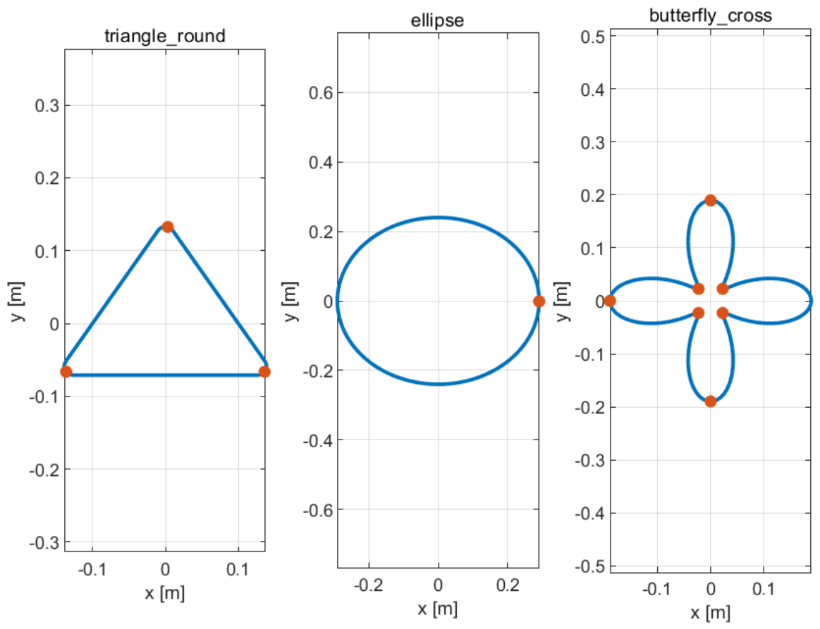
The rounded triangular contour is constructed from an equilateral triangular template with side length $l_{\mathrm{tri}}=0.30 \mathrm{m}$, followed by a vertical scaling factor of 0.82. The resulting vertex coordinates are (0, 0.1420) m, (−0.1500, −0.0710) m, and (0.1500, −0.0710) m. Each corner is rounded with a fillet radius of $r_{\mathrm{tri}}=0.012 \mathrm{m}$. After arc-length reparameterization, the total path length of the rounded triangular contour is $L_{\mathrm{tri}}=0.768705 \mathrm{m}$, and 900 discrete path samples are used.

The elliptical contour is generated from $x\left(\theta \right)=a_{\mathrm{ell}}\cos \theta$ and $y(\theta )=b_{\mathrm{ell}}\sin \theta ,$ where $\mathrm{\theta }\in \left[\left.0,2\mathrm{\pi }\right)\right.$. The semi-major and semi-minor axes are $a_{\mathrm{ell}}=0.29 \mathrm{m}$ and $b_{\mathrm{ell}}=0.24 \mathrm{m}$, respectively. The center is located at (0, 0), and the rotation angle is $0^{°}$. After arc-length reparameterization, the total path length of the elliptical contour is $L_{\mathrm{ell}}=1.668511 \mathrm{m}$, and 1200 discrete path samples are used.

The butterfly-cross contour is generated from the polar-form curve $r\left(\theta \right)=R_0+R_1\cos (n_{\mathrm{lobe}}\theta )$, $x\left(\theta \right)=r\left(\theta \right)\cos \theta$, and $y(\theta )=r(\theta )\sin \theta$, where $\mathrm{\theta }\in \left[\left.0,2\mathrm{\pi }\right)\right.$. The parameters are $R_0=0.11 \mathrm{m}$, $R_1=0.080 \mathrm{m}$, and $n_{\mathrm{lobe}}=4$. The x- and y-direction scaling factors are both set to 1.00, the center is located at (0, 0), and the rotation angle is $0^{°}$. After arc-length reparameterization, the total path length of the butterfly-cross contour is $L_{\mathrm{bf}}=1.513333 \mathrm{m}$, and 1400 discrete path samples are used.

In the present study, the compact execution-side relation in Equation (40) is adopted as the manuscript-level representation of the simulated downstream servo behavior. This model should be interpreted as an equivalent position-domain closed-loop servo-execution model rather than as a torque-level electromechanical model of a specific commercial motor-drive unit. Consequently, physical motor-drive parameters such as the equivalent mechanical inertia of the motor-driven axis, torque constant, current-loop dynamics, and Coulomb/viscous friction coefficients are not treated as separate independent simulation inputs. Their post-tuning influence is instead lumped into the equivalent closed-loop response $y_{\mathrm{nom}}\left(t\right)$, the normalized acceleration- and jerk-sensitivity coefficients $k_a$ and $k_j$, and the residual term $d\left(t\right)$.

More specifically, $y_{\mathrm{nom}}\left(t\right)$ represents the finite-bandwidth rigid closed-loop response of the axis, $k_a{\ddot{q}}_r\left(t\right)$ and $k_j{\stackrel{⃛}{q}}_r\left(t\right)$ represents the normalized sensitivity of the execution layer to acceleration and jerk transients, and $d\left(t\right)$ aggregates the flexible residual response, normalized internal disturbance forcing, small output-position disturbance, and output measurement noise. Therefore, Equation (40) is not an additional low-level controller design equation but a compact representation of the common closed-loop execution model used to evaluate all scheduling methods. Since all compared schedulers are tested under the same execution-side model, the observed differences in contouring accuracy, resonance-related excitation, and robustness can be attributed to the scheduling layer rather than to unequal actuator parameters or servo retuning.

The execution-side model in this study is intentionally formulated as a scheduler-oriented equivalent closed-loop response model rather than as a plant-identification-oriented full electromechanical servo model. This abstraction is adopted to isolate the influence of the feedrate scheduling layer on downstream contouring behavior under a common and controllable execution environment. In this model, the dominant execution-side mechanisms that are most relevant to reference-command quality are represented through finite bandwidth and damping, acceleration- and jerk-sensitive tracking-error channels, flexible residual dynamics, lumped disturbance inputs, generic measurement noise, and parameter mismatch.

This modeling choice improves the internal comparability among different schedulers because all methods are evaluated under the same execution-side dynamics and no method benefits from plant-specific servo retuning. Nevertheless, the present equivalent model does not explicitly parameterize all implementation-level servo nonidealities, such as Coulomb and viscous friction, mechanical backlash, drive saturation or current limiting, encoder quantization and resolution-dependent encoder noise, sampling delay, and communication delay. These factors may introduce additional tracking and contouring deviations in a physical biaxial platform. Therefore, the present results should be interpreted as scheduler-oriented simulation evidence under the considered equivalent execution conditions. Extending the current model toward a higher-fidelity servo representation that explicitly incorporates these implementation-level factors is an important direction for future work.

The possible influence of these unmodeled factors can be interpreted qualitatively. Coulomb and viscous friction may introduce nonlinear velocity-dependent tracking errors, especially near velocity reversals and low-speed bottleneck regions. In such regions, a smoother feedrate transition is expected to reduce abrupt acceleration and jerk demand and may therefore reduce friction-induced disturbance excitation. However, without physical friction identification, this effect should be regarded as a plausible tendency rather than a directly verified experimental conclusion. Mechanical backlash and axis coupling may also introduce additional contour-normal deviations, particularly when the two axes undergo repeated direction changes. These effects may partly weaken the quantitative gains reported in the present simulation, although the relative benefit of reducing aggressive feedrate transitions is still expected to remain relevant because such transitions generally increase the burden on coupled mechanical dynamics.

The single flexible residual mode used in the present equivalent model should also be understood as a simplified representation of resonance-sensitive behavior. A real gantry or XY motion stage may contain multiple structural modes with different damping ratios and mode shapes. If the actual dominant modes are located away from the selected resonance-sensitive band or have stronger damping, the absolute value of E(HF) and the magnitude of the contour-error reduction may become smaller. Conversely, if a lightly damped mode lies close to the high-frequency content generated by aggressive scheduling, the benefit of smoother feedrate transitions may become more pronounced. Sampling delay, communication delay, encoder quantization, and drive saturation may further enlarge tracking lag or introduce nonlinear clipping effects. These factors may reduce the direct quantitative transferability of the current results to a specific physical platform, but they do not change the main scheduler-level implication that reducing concentrated jerk and resonance-sensitive excitation is beneficial for execution robustness. Therefore, the present conclusions should be interpreted as simulation-based evidence of the scheduling mechanism, while hardware-calibrated servo modeling and experimental validation are required before claiming platform-specific performance gains.

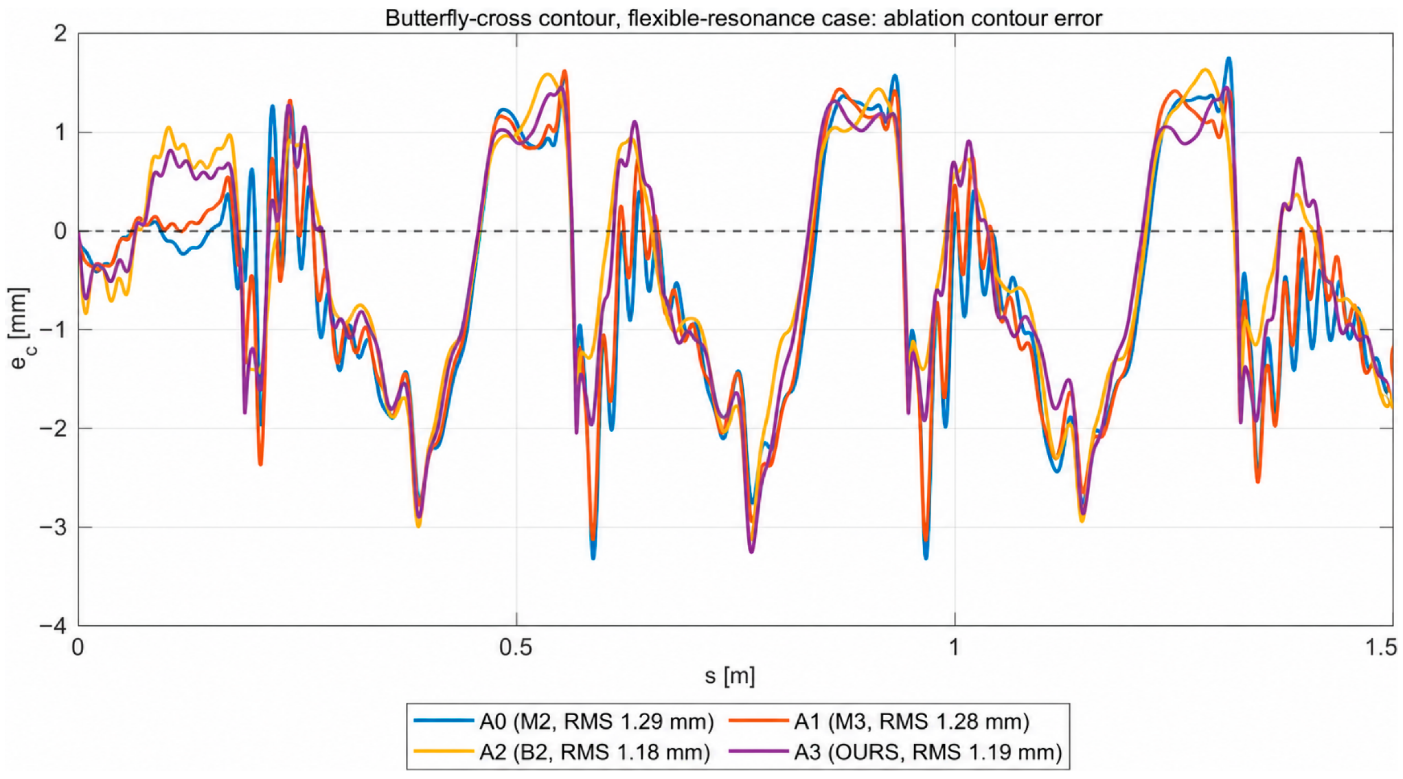
Five compared feedrate scheduling methods are considered in this study, denoted as M2, M3, B1, B2, and OURS. It should be emphasized that M2, M3, B1, and B2 are constructed reference schedulers used for internally controlled comparison rather than strict one-to-one reproductions of specific published algorithms. Specifically, M2 is an acceleration-limited reference scheduler inspired by admissible feedrate generation and constrained time-scaling strategies under velocity and tangential-acceleration bounds [18,22]. M3 extends this acceleration-feasible backbone by introducing jerk-oriented smoothing, following the general ideas of jerk-limited trajectory generation and jerk-aware time scaling [17,25]. B1 represents geometry-oriented smoothing and look-ahead profile-blending behavior adapted from representative constrained motion scheduling strategies [23,24]. B2 represents an optimization-like error-aware reshaping strategy inspired by execution-sensitive contouring compensation and time-accuracy tradeoff-oriented scheduling ideas [8,28]. Therefore, these four reference schedulers are used to represent representative classes of scheduling mechanisms, including acceleration feasibility, jerk regularization, geometry-oriented smoothing, look-ahead profile blending, and execution/error-aware feedrate reshaping. They are not intended to serve as exact benchmark implementations of individual public algorithms. OURS denotes the proposed execution-aware feedrate scheduler, which combines admissibility-aware baseline generation, jerk-oriented smoothness refinement, and critical-region-preserving correction.

Although all methods follow the same geometric contours and are evaluated under the same downstream execution conditions, they generate different timing laws and therefore exhibit different tradeoffs among traversal time, motion smoothness, contouring accuracy, and robustness. The hyperparameters of the competing baselines were tuned to achieve their best nominal contouring performance under the common evaluation setting before the final comparison was conducted.

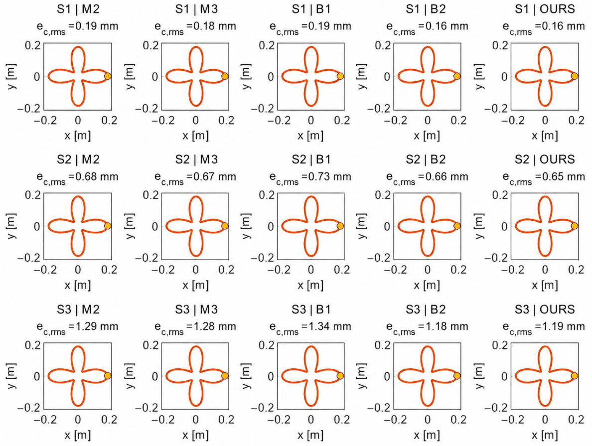
Four execution-related operating conditions are considered in the simulations. The first condition is the nominal case S1, in which the equivalent rigid-loop dynamics are characterized by natural frequencies of $34 \mathrm{rad}/\mathrm{s}$ and $32 \mathrm{rad}/\mathrm{s}$ for the $x$- and $y$-axes, respectively, with damping ratios of 0.78 and 0.74. The flexible residual component is characterized by a representative frequency of $44 \mathrm{Hz}$, a damping ratio of 0.080, and a dimensionless normalized flexible-coupling scale ${\gamma }_f=0.35$. The normalized disturbance forcing amplitude is $A_d=0.015$, the disturbance frequency is $f_d=7.0$ Hz, and the output-position measurement-noise standard deviation is ${\sigma }_n=2\times {10}^{-6} \mathrm{m}$.

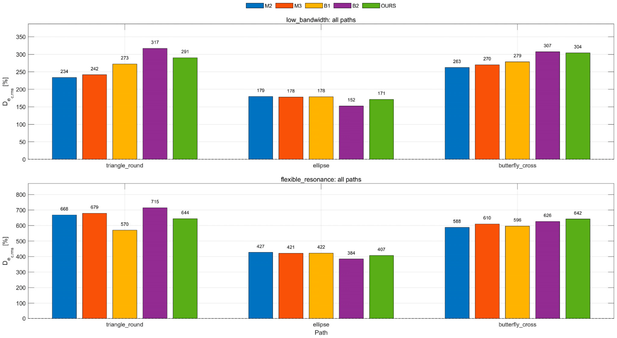
The second condition is the low-bandwidth case S2, where the equivalent rigid-loop natural frequencies are reduced to $26 \mathrm{rad}/\mathrm{s}$ and $24 \mathrm{rad}/\mathrm{s}$ for the $x$- and $y$-axes, respectively, while the damping ratios are reduced to 0.70 and 0.66. The flexible residual component is described by $f_f=42$ Hz, ${\zeta }_f=0.060$, and ${\gamma }_f=0.55$. The normalized disturbance forcing amplitude is $A_d=0.020$, the disturbance frequency is $f_d=7.5$ Hz, and the output-position measurement-noise standard deviation is ${\sigma }_n=3\times {10}^{-6}\mathrm{m}$. This condition is used to emulate weakened servo responsiveness.

The third condition is the flexible-resonance case S3, in which the equivalent rigid-loop natural frequencies are further reduced to $22 \mathrm{rad}/\mathrm{s}$ and $20 \mathrm{rad}/\mathrm{s}$ for the $x$- and $y$-axes, respectively, with damping ratios of 0.64 and 0.60. A more prominent lightly damped flexible residual component is superposed, with $f_f=45 \mathrm{Hz}$, ${\zeta }_f=0.030$, and ${\gamma }_f=0.95$. The normalized disturbance forcing amplitude is $A_d=0.030$, the disturbance frequency is $f_d=8.0 \mathrm{Hz}$, and the output-position measurement-noise standard deviation is ${\sigma }_n=4\times {10}^{-6} \mathrm{m}$. This condition is used to examine whether different schedulers inject resonance-sensitive command components.

Here, ${\gamma }_f$ is not a physical motor or controller gain. It is a dimensionless normalized coupling scale used to adjust the contribution of the flexible residual component included in the lumped term $d\left(t\right)$ of Equation (40). Similarly, $A_d$ denotes the normalized forcing amplitude injected into the equivalent execution model, whereas ${\sigma }_n$ denotes the standard deviation of the output-position measurement noise in meters. These definitions are introduced to avoid interpreting the equivalent execution parameters as the physical equivalent inertia, torque constant, friction coefficient, or real servo-loop gains of a specific commercial actuator.

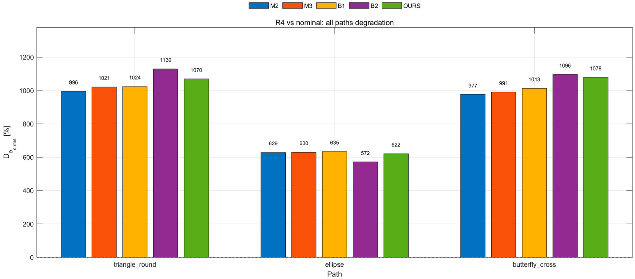
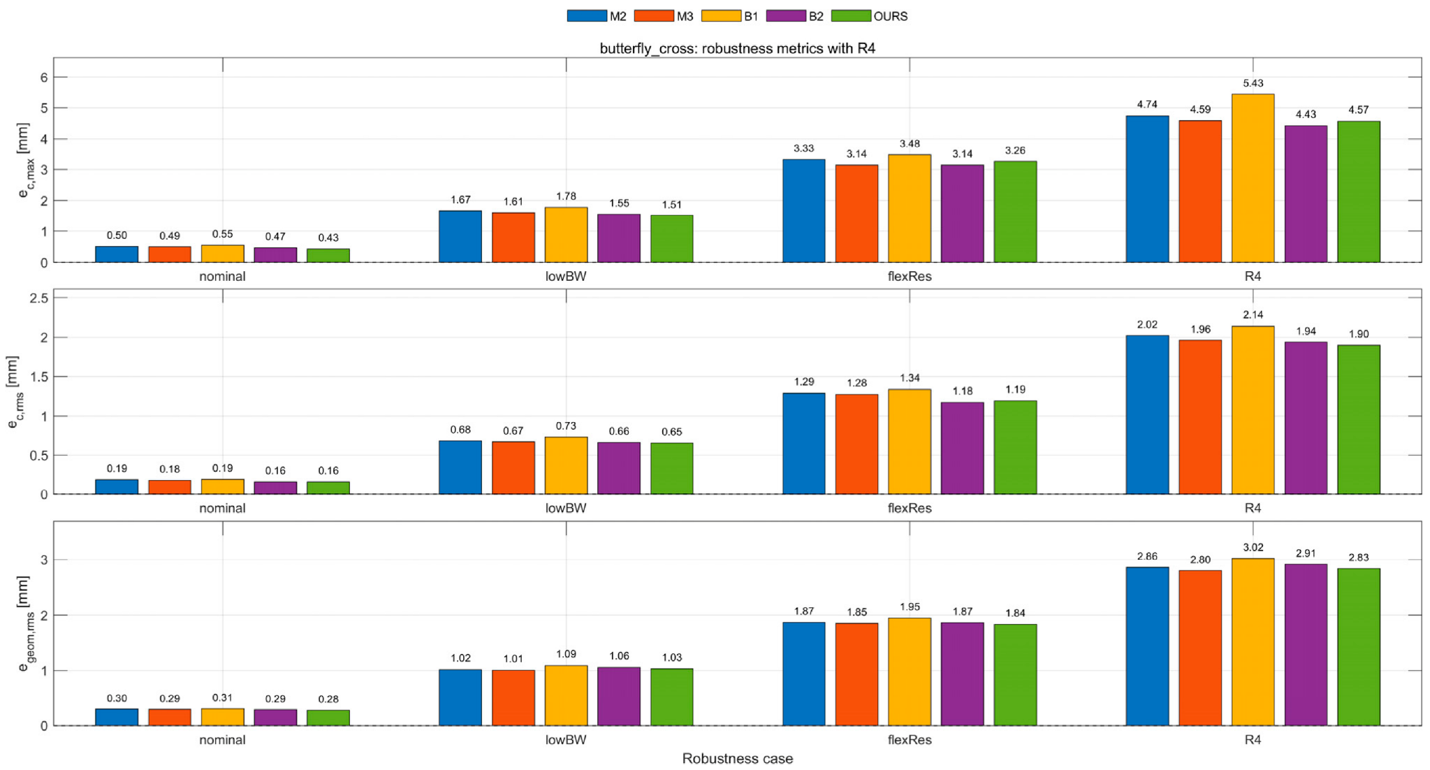
In addition, a parameter-mismatch case R4 is introduced in the robustness study. In this case, a deliberate mismatch is imposed between the nominal planning-side model and the simulated execution-side response. Specifically, the equivalent execution bandwidth is scaled by 1.32 relative to the nominal assumption, the damping level is reduced to 0.78 of the nominal value, and the normalized acceleration- and jerk-sensitivity coefficients $k_a$ and $k_j$ in the equivalent execution model are increased from 2.20 to 5.60 and from 0.70 to 1.65, respectively. The flexible residual coupling included in $d\left(t\right)$ is also strengthened. Therefore, R4 represents a compound equivalent execution-side mismatch, under which the simulated execution model becomes more sensitive to aggressive acceleration and jerk transients than assumed in the nominal planning-side setting.

From a modeling viewpoint, S2 is implemented by reducing the equivalent rigid-loop bandwidth and damping of both axes relative to the nominal condition so that the same reference timing law becomes more difficult to realize in closed-loop execution. By contrast, S3 is implemented not only by further weakening the rigid channel but also by introducing a stronger lightly damped flexible residual component near the resonance-sensitive frequency band. As a result, S2 mainly represents reduced command-following capability, whereas S3 represents vibration-sensitive execution in which aggressive acceleration and jerk transitions are more easily amplified into contour-normal deviation. R4 further extends this setting by introducing an explicit mismatch between the nominal planning-side assumption and the simulated execution-side response, thereby allowing the robustness of different schedulers to be examined under nonnegligible model inconsistency.

The global simulation and scheduling parameters used throughout this study are summarized in

Table 1. Global simulation parameters and evaluation settings.

Symbol/Item	Meaning	Value	Unit
$V_{\max }$	Maximum feedrate	2.0	m/s
$A_{\tan ,\max }$	Tangential acceleration limit	1.60	m/${\mathrm{s}}^2$
$A_{\mathrm{n},\max }$	Normal acceleration limit	0.08	m/${\mathrm{s}}^2$
$J_{\max }$	Jerk limit	8.0	m/${\mathrm{s}}^3$
${ϵ}_{\kappa }$	Curvature regularization term	1 × ${10}^{-6}$	–
$v_{\mathrm{floor}}$	Minimum admissible feedrate floor	0.12	m/s
$N_{\mathrm{tri}}$	Path samples for rounded triangle	900	–
$N_{\mathrm{ell}}$	Path samples for ellipse	1200	–
$N_{\mathrm{bf}}$	Path samples for butterfly-cross	1400	–
$N_{\mathrm{search}}$	Projection search window for contour-error evaluation	80	pts
$f_{\mathrm{HF}}$	High-frequency analysis band	20–100	Hz
$f_{\mathrm{r}}$	Resonance-sensitive band	35–55	Hz
FFT rule	Spectral analysis length selection	nextpow2	–

, whereas the operating-condition variations for S2, S3, and R4 are specified separately in the corresponding execution-setting descriptions. Unless otherwise stated, these parameters are kept fixed for all compared methods and all test contours so that the observed performance differences can be attributed to the structural differences in scheduling design rather than to inconsistent constraint or sampling settings.

The operating-condition-dependent servo parameters are not repeated in Table 1. Instead, they are reported directly in the definitions of S1, S2, S3, and R4, including the rigid-loop natural frequencies and damping ratios, the flexible-mode settings, and the mismatch-related sensitivity coefficients. In this way, Table 1 reports the globally fixed simulation and scheduling parameters, while the execution-condition variations remain explicitly associated with their corresponding operating cases.

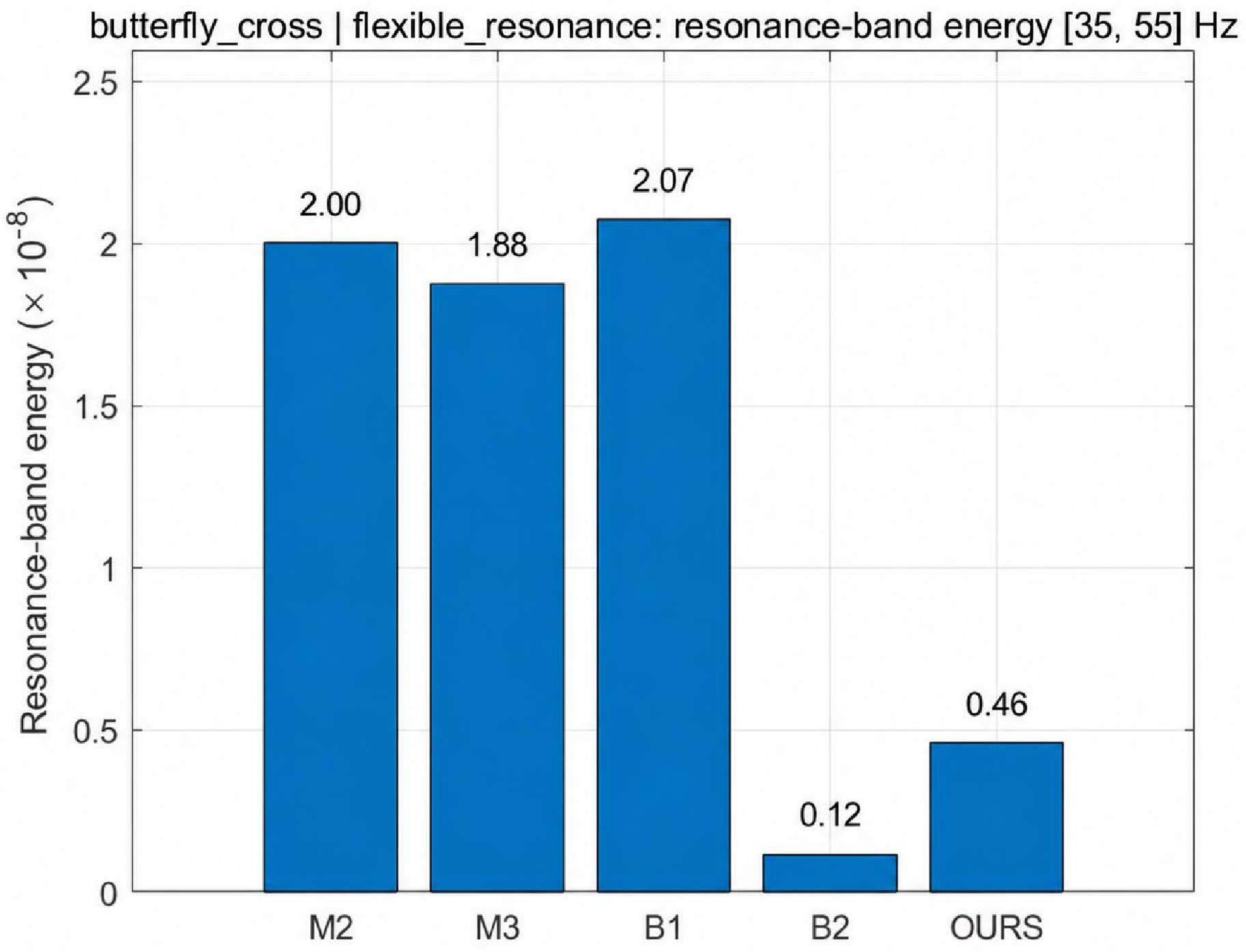
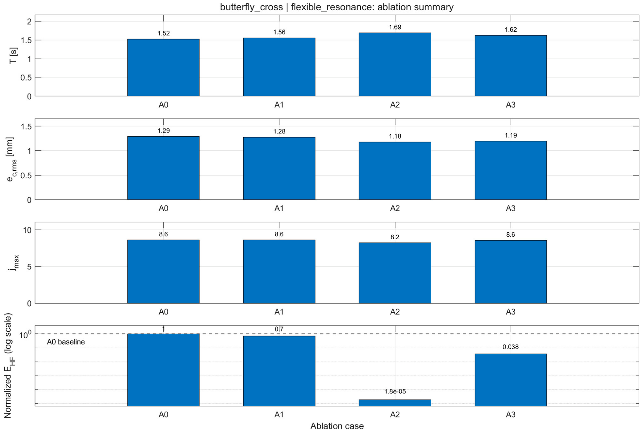
The frequency bands used for E(HF) and resonance-sensitive interpretation are selected according to the equivalent flexible-resonance setting adopted in the simulation model. The 35–55 Hz band is centered around the representative flexible residual mode introduced in S3, whose nominal frequency is approximately 45 Hz. A ±10 Hz interval is used to cover moderate uncertainty of the equivalent resonance location and the spectral spreading caused by finite-duration acceleration and jerk transitions. The broader 20–100 Hz band is used as a high-frequency command-excitation band to capture acceleration-spectrum content that is above the dominant low-frequency traversal component but still relevant to the lightly damped flexible response considered in the simulation. Therefore, the 35–55 Hz band is used mainly for resonance-sensitive interpretation, whereas the 20–100 Hz band is used to evaluate the overall high-frequency excitation tendency of the reconstructed acceleration commands. These bands should not be interpreted as universal physical frequency ranges for all biaxial gantry systems. For a specific hardware platform, the corresponding bands should be determined or adjusted according to experimentally identified modal frequencies, servo bandwidth, sampling rate, and structural damping.

The evaluation metrics are organized into three groups. The first group contains geometric and contouring indicators, including contouring error $e_c$, tangential error $e_t$, contour-error root-mean-square value $e_{c, \mathrm{rms}}$, and geometric root-mean-square error $e_{\mathrm{geom},\mathrm{rms}}$, which reflect the final contouring quality in closed-loop execution. The second group contains kinematic smoothness indicators, such as feedrate evolution, acceleration response, jerk behavior, and peak jerk $j_{\mathrm{peak}}$, which characterize the transient severity of the generated timing law. These kinematic quantities are computed with respect to time, whereas local waveform comparisons are presented against the corresponding arc-length coordinate $s$ when different methods have different traversal times. This path-domain presentation avoids the misalignment caused by unequal total execution times and enables local transitions to be compared at the same geometric positions. The third group contains robustness-related indicators, including performance degradation under bandwidth reduction, flexible resonance, and parameter mismatch. In this way, the effectiveness of each method is not judged only by nominal path-domain admissibility or execution time but by its overall behavior throughout the planning-to-execution chain.

To ensure a fair comparison, all five methods are evaluated under the same contour set, the same motion constraints, the same resampling interval, and the same downstream execution-side conditions. In particular, the maximum feedrate $V_{\max }$, admissible acceleration limits $A_{\tan ,\max }$ and $A_{\mathrm{n},\max }$, jerk bound $J_{\max }$, and sampling interval are kept identical for M2, M3, B1, B2, and OURS throughout the simulations. Therefore, no method benefits from relaxed kinematic constraints, denser sampling, or condition-specific servo retuning. The observed performance differences are thus attributed to the structural differences in scheduling design rather than to artificially favorable simulation settings. In addition, the hyperparameters of the advanced baseline and the proposed method are fixed globally rather than retuned for each contour or each operating condition. This setting is intentionally adopted to prevent case-by-case bias and to examine whether the scheduler structure itself can maintain stable performance across different geometric patterns and execution environments.

Accordingly, the comparative results reported in the following subsections should be interpreted under the present composite baseline construction and unified evaluation conditions rather than as a claim of universal superiority over all possible implementations of the corresponding public scheduling algorithms.

4.3. Feedrate and Kinematic Planning Results

This subsection first examines the path geometry and the corresponding feedrate scheduling results. The purpose is to determine whether the proposed method can generate smoother motion commands without violating the prescribed admissible feedrate boundary. In this analysis, attention is paid not only to the final traversal time $T$ but also to the local feedrate transition, acceleration behavior, and jerk response because these quantities directly affect the subsequent closed-loop contouring performance.

The three reference contours and representative critical points are shown in Figure 1. The rounded triangular contour contains several localized high-curvature regions, while the ellipse has a relatively smooth geometric variation. The butterfly-cross contour is more challenging because it contains repeated turning-direction changes and multiple path-critical regions. Therefore, these three contours provide a progressive test set for evaluating the proposed scheduler under different levels of geometric complexity.

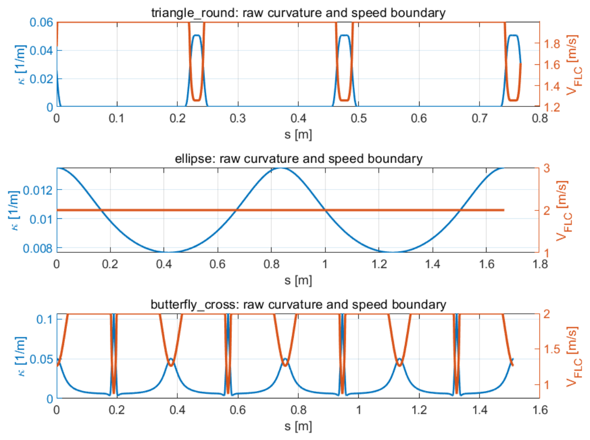
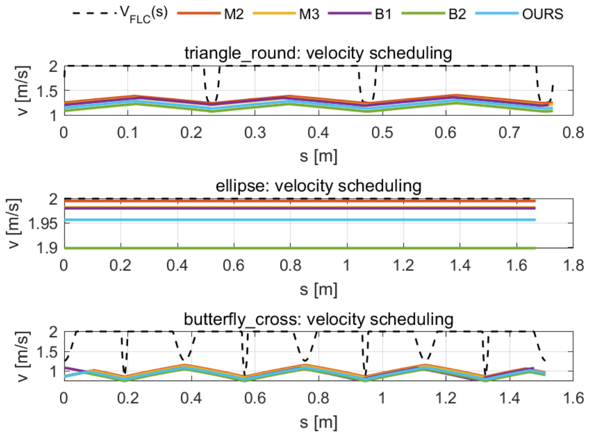
The curvature distributions and the corresponding admissible feedrate boundaries are shown in Figure 2. For the ellipse, the curvature variation is relatively mild, and thus the admissible feedrate boundary changes smoothly. For the rounded triangle and the butterfly-cross contour, the boundary exhibits more pronounced local reductions near high-curvature regions. These local reductions indicate that the scheduler must slow down near path-critical segments to satisfy the geometric and motion constraints. Therefore, the key difficulty is not only to respect the boundary but also to connect different speed levels smoothly across adjacent path segments.

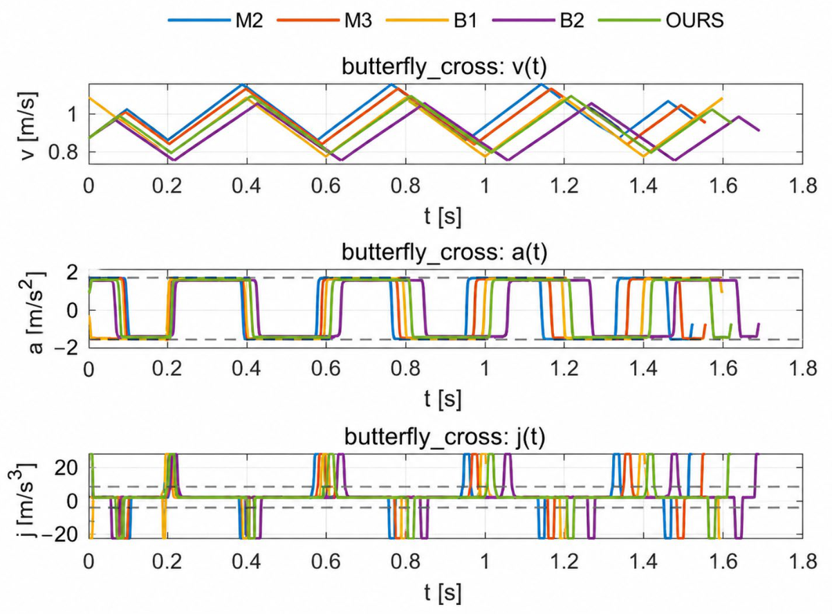
The scheduled feedrate profiles of different methods are compared in Figure 3. The more aggressive methods tend to stay closer to the admissible boundary and therefore obtain shorter traversal time. However, this behavior is accompanied by sharper local speed transitions. By contrast, smoother methods back off from the boundary more conservatively and produce more rounded feedrate evolution across consecutive bottlenecks. The main implication is that the planning-layer advantage of smoother methods does not lie in higher speed utilization but in weaker excitation concentration.

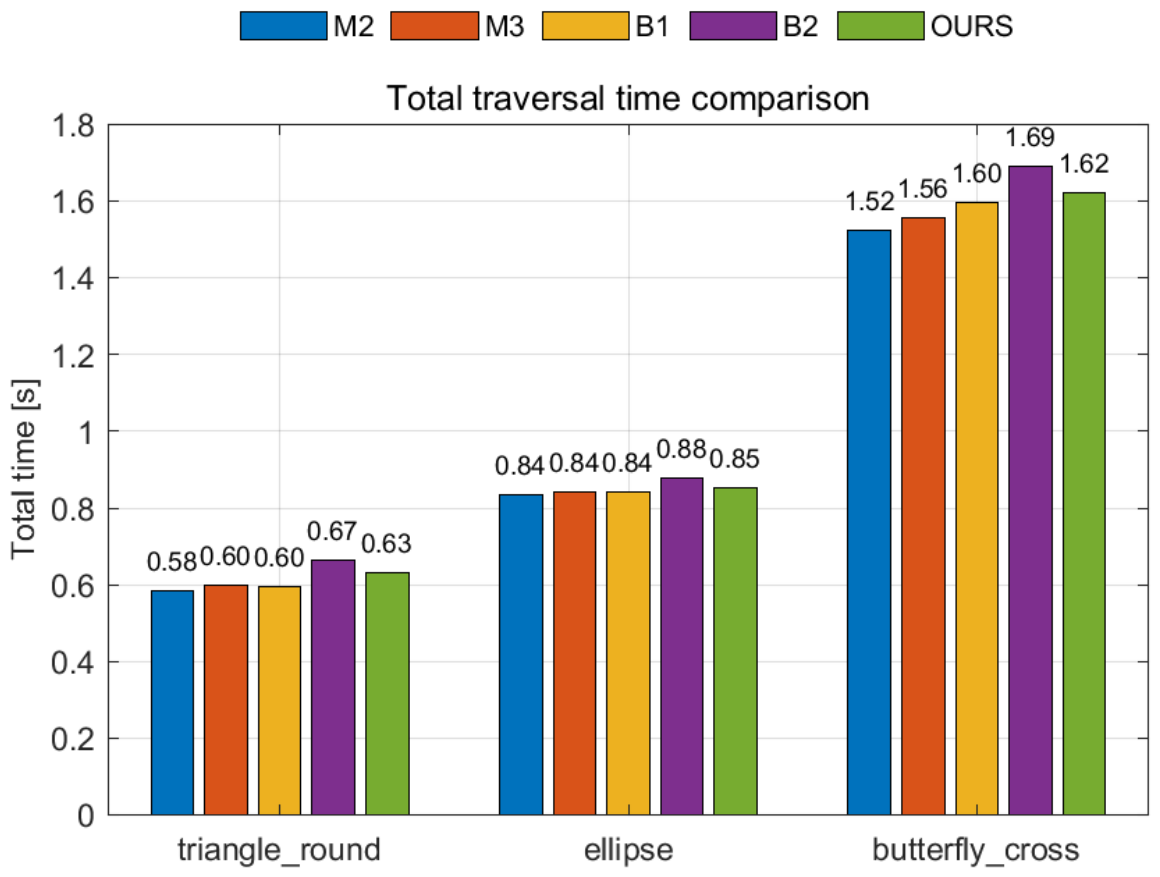
This tradeoff becomes clearer in the comparison of the total traversal time T, as shown in Figure 4. The more aggressive methods generally achieve the shortest execution time, whereas the smoother methods, including the proposed method, exhibit slightly longer traversal duration. Therefore, based on T alone, the proposed method should not be described as globally superior. Instead, its traversal-time increase should be interpreted as the efficiency cost paid for smoother local feedrate transitions and improved downstream contouring behavior. From the viewpoint of machining efficiency, a shorter traversal time is beneficial for productivity, but it may also require more abrupt acceleration and deceleration switching near path-critical regions, thereby increasing jerk-sensitive excitation and degrading contouring accuracy during servo execution. The proposed method is designed to avoid this purely time-aggressive behavior and to seek a more balanced tradeoff among traversal efficiency, jerk suppression, and contour-following accuracy.

As shown in Figure 5, the time-domain kinematic comparison further clarifies the differences among methods. On the representative butterfly-cross contour, the velocity trajectories of the smoother methods evolve more gradually, while their acceleration and jerk responses $a\left(t\right)$ and $j\left(t\right)$ contain less abrupt switching behavior. In particular, the proposed method suppresses concentrated jerk bursts around repeated bottleneck transitions. This observation is important because repeated local jerk concentration is precisely what tends to excite flexible dynamics and amplify contour deviation during later closed-loop execution. Therefore, the planning-layer conclusion of this subsection is limited but clear: the proposed method produces smoother execution-oriented commands and weaker high-frequency excitation at the cost of a moderate increase in traversal time.

4.4. Contouring Performance Under Nominal Condition

After examining the planning-layer results, the next question is whether the smoother timing laws actually improve contour-following quality in closed-loop execution. As shown in the first row of Figure 6, all methods remain capable of following the desired contour under the nominal servo condition, but their deviations are not identical. The differences become more visible on the butterfly-cross contour, where repeated direction changes and curvature concentration make the contouring task more demanding. In this case, the smoother methods maintain executed contours that remain closer to the planned path, indicating that reducing command aggressiveness can improve execution consistency even when the servo condition is nominal.

As shown in Figure 7,the contouring error $e_c$ and tangential error $e_t$ further support this observation. Since different scheduling methods complete the butterfly-cross contour with different traversal times, these error signals are presented in the path domain using the arc-length coordinate $s$. In this way, the error responses of different methods are compared at the same geometric locations along the contour rather than at the same elapsed time. Although the tangential errors of the compared methods remain within a similar range, the contour-error evolution exhibits more pronounced differences near repeated path-critical segments. The proposed method does not simply shift the error from one coordinate direction to another. Instead, it reduces the more execution-critical contour-normal deviation while preserving comparable tangential behavior. This distinction is important because practical contour-following quality is governed primarily by the normal deviation from the desired contour rather than by tangential phase lag alone.

Therefore, the nominal-condition results provide the first closed-loop justification for the proposed scheduling framework. The smoother commands obtained in Section 4.3 are not merely visually smoother or spectrally milder; they also translate into smaller contour-normal deviation during simulated closed-loop contour execution. This means that the moderate traversal-time penalty observed in the planning layer is partly compensated by improved contour-following quality in the servo loop. Accordingly, the value of the proposed method should be interpreted as an execution-oriented smoothness-accuracy tradeoff rather than as a purely time-optimal design.

4.5. Frequency-Domain Interpretation of Contouring Performance

The nominal closed-loop results indicate that smoother scheduling leads to smaller contour deviation, but this improvement still requires a physical interpretation. For this reason, the present subsection analyzes the resonance-band energy $E_{\mathrm{HF}}$ on the representative butterfly-cross contour under the flexible-resonance condition. The purpose is not to introduce an additional independent performance target but to explain why some scheduling strategies deteriorate more severely when the servo system becomes vibration-sensitive.

As shown in Figure 8, the resonance-band energy comparison shows a clear separation among methods. The more aggressive strategies produce substantially larger energy concentration inside the resonance-sensitive frequency interval, whereas the smoother strategies, especially B2 and OURS, suppress this concentration more effectively. Since flexible contouring performance depends not only on low-frequency path-following ability but also on whether the command injects energy near the structural resonance range, the reduction of $E_{\mathrm{HF}}$ provides a direct explanation for the smaller contour RMS error observed for smoother methods in later robustness tests.

This frequency-domain observation also helps connect Section 4.3 and Section 4.4. In Section 4.3, the proposed method exhibited weaker jerk concentration and more gradual transition across bottleneck regions. In Section 4.4, it yielded smaller contour-normal deviation under nominal closed-loop execution. The present spectral result explains the link between these two observations: smoother command evolution weakens excitation around vibration-sensitive frequencies, which in turn reduces the amplification of contour deviation during servo execution. Therefore, the advantage of the proposed method should not be interpreted as a purely geometric planning effect but as a joint consequence of smoother timing law and reduced resonance-oriented excitation.

4.6. Robustness and Parameter-Mismatch Analysis

The results above were obtained either at the planning layer or under nominal closed-loop execution. A more demanding question is whether the relative advantage of smoother scheduling can be preserved when the servo system becomes less favorable. This tendency can already be qualitatively observed from the second and third rows of Figure 6, where the discrepancies between the planned and executed contours become more pronounced under the low-bandwidth and flexible-resonance conditions. This subsection therefore considers three nonnominal situations, namely low bandwidth, flexible resonance, and parameter mismatch. The discussion is organized from qualitative contour distortion to quantitative degradation statistics.

As shown in Figure 9, a first quantitative observation is provided by the all-path degradation summary under the low-bandwidth and flexible-resonance conditions. Relative to the nominal case, all methods suffer noticeable growth in contour RMS error $e_{\mathrm{c}, \mathrm{rms}}$, but the severity of this growth is strongly path-dependent. The ellipse remains comparatively benign, whereas the rounded triangle and the butterfly-cross contour both exhibit substantially larger sensitivity. This confirms that robustness cannot be judged solely from nominal tracking quality but must be evaluated jointly with path geometry and servo deterioration.

As shown in Figure 10, the parameter-mismatch case R4 further extends the robustness evaluation by introducing an explicit discrepancy between the nominal planning-side model and the simulated execution-side response. In this case, the equivalent execution bandwidth is scaled by 1.32 relative to the nominal reference, the damping level is reduced to 0.78 of the nominal value, the acceleration- and jerk-sensitivity coefficients $k_a$ and $k_j$ in the equivalent execution model are increased from 2.20 to 5.60 and from 0.70 to 1.65, respectively, and the flexible-channel coupling is also strengthened. This setting is intended to represent a compound execution-side mismatch, under which the execution-side model becomes more sensitive to aggressive acceleration and jerk transients than assumed in the nominal planning model. Therefore, R4 is used to evaluate whether the compared schedulers can still preserve acceptable contouring quality when non-negligible deviation exists between the nominal assumption and the execution-side dynamics.

As shown in Figure 11, a more detailed view is obtained from the robustness metrics of the representative butterfly-cross contour. Across the nominal, low-bandwidth, flexible-resonance, and R4 cases, both contour RMS error $e_{\mathrm{c}, \mathrm{rms}}$ and geometric RMS error $e_{\mathrm{geom},\mathrm{rms}}$ increase when the servo condition deteriorates, but the magnitude of deterioration is not uniform across methods. The smoother scheduling strategies retain a more controlled error-growth trend, whereas the more aggressive baselines exhibit stronger sensitivity to bandwidth reduction, resonance amplification, and parameter mismatch. This again indicates that excitation suppression plays a central role in practical robustness.

Taken together, these results lead to a more complete robustness interpretation of the proposed method. First, nonnominal servo conditions do not affect all paths equally; complex contours degrade more severely. Second, flexible-resonance and parameter-mismatch conditions cause substantially stronger deterioration than nominal or mildly weakened cases. Third, the relative advantage of smoother scheduling becomes more meaningful under adverse conditions than under nominal execution, because robustness depends strongly on excitation suppression rather than only on nominal path-tracking capability. Therefore, the proposed method should be viewed not simply as a nominal-condition smoother scheduler but as a planning strategy whose main value becomes more evident when the execution environment deteriorates.

To examine whether the robustness trends are dependent on a single deterministic realization, an additional multi-run variability analysis was conducted on the butterfly-cross contour under the nonnominal execution conditions S2, S3, and R4. For each condition, ten independent realizations were generated by changing the disturbance and measurement-noise seeds in the equivalent execution model. In the R4 parameter-mismatch case, small random perturbations were also introduced to the normalized acceleration- and jerk-sensitivity coefficients $k_a$ and $k_j$ around their nominal mismatch values. The feedrate schedule of each method was kept unchanged so that the reported variability mainly reflects the influence of execution-side disturbance, measurement noise, and mismatch perturbation rather than case-specific retuning of the scheduler.

The resulting mean ± standard deviation values of e(c, rms), j(peak), E(HF), and T are summarized in

Table 2. Multi-run statistical summary on the butterfly-cross contour under S2, S3, and R4.

Condition	Method	e(c, rms) [mm]	j(peak) [m/s3]	E(HF) [−]	T [s]
S2	M2	0.6977 ± 0.0090	8.6400 ± 0.0000	0.0000000026469 ± 0.000000000000000016289	1.5246 ± 0.0000
S2	M3	0.6769 ± 0.0062	8.6399 ± 0.0000	0.0000000020103 ± 0.000000000000000017568	1.5577 ± 0.0000
S2	B1	0.7283 ± 0.0020	8.6400 ± 0.0000	0.0000000028107 ± 0.0000000000000000084605	1.5978 ± 0.0000
S2	B2	0.6495 ± 0.0105	8.2418 ± 0.0000	0.00000000030683 ± 0.0000000000000000090554	1.6924 ± 0.0000
S2	OURS	0.6471 ± 0.0048	8.5804 ± 0.0000	0.00000000052886 ± 0.0000000000000000075549	1.6228 ± 0.0000
S3	M2	1.2695 ± 0.0125	8.6400 ± 0.0000	0.000000013953 ± 0.00000000000000012579	1.5246 ± 0.0000
S3	M3	1.2398 ± 0.0099	8.6399 ± 0.0000	0.000000010815 ± 0.00000000000000026934	1.5577 ± 0.0000
S3	B1	1.3441 ± 0.0292	8.6400 ± 0.0000	0.000000013938 ± 0.00000000000000043912	1.5978 ± 0.0000
S3	B2	1.2087 ± 0.0282	8.2418 ± 0.0000	0.0000000017105 ± 0.000000000000000015071	1.6924 ± 0.0000
S3	OURS	1.2061 ± 0.0303	8.5804 ± 0.0000	0.0000000031928 ± 0.00000000000000010288	1.6228 ± 0.0000
R4	M2	2.0515 ± 0.0472	8.6400 ± 0.0000	0.000000047520 ± 0.0000000013456	1.5246 ± 0.0000
R4	M3	1.9886 ± 0.0322	8.6399 ± 0.0000	0.000000037370 ± 0.00000000070915	1.5577 ± 0.0000
R4	B1	2.1684 ± 0.0328	8.6400 ± 0.0000	0.000000047074 ± 0.0000000012668	1.5978 ± 0.0000
R4	B2	1.9115 ± 0.0381	8.2418 ± 0.0000	0.0000000042153 ± 0.00000000016999	1.6924 ± 0.0000
R4	OURS	1.9034 ± 0.0272	8.5804 ± 0.0000	0.0000000092342 ± 0.00000000037819	1.6228 ± 0.0000

. The statistical results show that the main robustness trends observed in the single-run results are preserved across repeated realizations. Under S2 and S3, the proposed method maintains the lowest or comparable mean contour RMS error among the compared methods. Under R4, the proposed method also gives the lowest mean e(c, rms), while B2 gives the lowest E(HF). This indicates that the proposed scheduler does not dominate every single metric but provides a more balanced compromise between contouring accuracy, resonance-sensitive excitation, and traversal time. The standard deviations of T and j(peak) are nearly zero because the feedrate schedules and reference jerk profiles are deterministic, while only the execution-side disturbance, noise, and mismatch realizations are varied. The standard deviation of E(HF) is also very small in S2 and S3 because the integrated frequency-band energy is mainly determined by the deterministic reference command and equivalent flexible channel. These results indicate that the robustness conclusions are not caused by a single favorable disturbance realization.

4.7. Ablation Study

To further examine whether the retained design elements of the proposed scheduling framework are structurally meaningful, an ablation study was conducted on the representative butterfly-cross contour under the flexible-resonance condition. Four ablation configurations, denoted as A0–A3, were compared from the perspectives of jerk behavior, contouring error, execution time, and high-frequency excitation. The purpose of this subsection is not merely to rank different reduced variants but to clarify how the removal or weakening of specific smoothness-oriented design elements changes the final contouring behavior of the system.

The jerk-level differences among the ablation configurations are first shown in Figure 12. Since different ablation configurations lead to different traversal times, the jerk responses are plotted against the arc-length coordinate $s$ rather than the time coordinate $t$. The jerk values are still computed as time derivatives, but the path-domain presentation allows the transient behavior to be compared at consistent geometric locations. A0 and A1 exhibit the most pronounced oscillatory and switching-like jerk behavior near repeated path-critical segments, indicating that the corresponding motion commands still contain substantial transient excitation. A3 yields a visibly smoother overall jerk evolution than A0 and A1, whereas A2 achieves the smallest peak jerk among the four configurations. This result shows that the smoothness-related design elements removed or weakened in the ablation process have a direct impact on the high-frequency aggressiveness of the generated motion command.

The contour-error comparison in Figure 13 further shows that these jerk-level differences are not merely superficial waveform changes. The contour-error responses are also plotted against the arc-length coordinate $s$ so that deviations caused by different ablation configurations can be compared at the same geometric locations. A0 and A1 exhibit larger and less regular contour deviation over repeated local segments of the trajectory, whereas A2 and A3 maintain smaller contour-error levels and a more controlled error envelope. This observation supports the view that the retained smoothness-oriented design elements do not simply reshape the command profile but also influence the final contour-following quality through their effect on transient excitation.

The overall tradeoff among the ablation configurations is summarized in Figure 14. A2 attains the smallest contour RMS error, the smallest peak jerk, and the lowest normalized resonance-band energy, but it also incurs the longest traversal time. By contrast, A0 achieves the shortest traversal time but with larger contour error and stronger high-frequency excitation. Although A3 does not minimize every individual metric, it provides a more balanced compromise among execution efficiency, contouring accuracy, and excitation suppression. This result further confirms that the proposed framework should not be evaluated from a single-objective minimum-time perspective. A configuration that minimizes traversal time may retain stronger jerk bursts and higher resonance-band excitation, whereas a configuration that minimizes jerk and contour error may introduce a larger traversal-time penalty. Therefore, the practically useful solution is not necessarily the fastest or the smoothest individual profile but the one that provides an acceptable compromise among productivity, command smoothness, and contouring accuracy. The quantitative comparison in Figure 14 shows this tradeoff explicitly by jointly considering traversal time, contour RMS error, peak jerk, and normalized resonance-band energy. This also explains why the proposed scheduler is described as an execution-aware smoothness–accuracy tradeoff method rather than as a purely time-optimal feedrate planner. Therefore, the ablation study supports the structural necessity of the complete scheduling framework adopted in this work.

A similar multi-run check was also conducted for the ablation configurations A0–A3 on the butterfly-cross contour under the flexible-resonance condition. The mean ± standard deviation results are summarized in

Table 3. Multi-run statistical summary for ablation configurations A0–A3 on the butterfly-cross contour under S3.

Configuration	Source Method	e(c, rms) [mm]	j(peak) [m/s3]	E(HF) [−]	T [s]
A0	M2	1.2710 ± 0.0099	8.6400 ± 0.0000	0.000000013953 ± 0.00000000000000011680	1.5246 ± 0.0000
A1	M3	1.2552 ± 0.0222	8.6399 ± 0.0000	0.000000010815 ± 0.00000000000000029093	1.5577 ± 0.0000
A2	B2	1.2043 ± 0.0182	8.2418 ± 0.0000	0.0000000017105 ± 0.000000000000000016743	1.6924 ± 0.0000
A3	OURS	1.1932 ± 0.0192	8.5804 ± 0.0000	0.0000000031928 ± 0.000000000000000082153	1.6228 ± 0.0000

. The repeated simulations confirm that the ablation trend remains stable. Compared with A0 and A1, the configurations with stronger execution-aware reshaping or critical-region-preserving correction reduce the mean contour RMS error and resonance-sensitive energy. A3 achieves the lowest mean e(c, rms) and a shorter traversal time than A2, whereas A2 gives the lowest E(HF). Therefore, the full proposed configuration should be interpreted as a balanced design rather than a component that minimizes every individual index. This confirms that the ablation conclusion is not dependent on a single realization of the execution-side disturbance.

4.8. Parameter-Sensitivity Analysis

To further examine whether the reported robustness and tradeoff conclusions are dependent on the selected execution-side parameters, an additional compact parameter-sensitivity analysis was conducted on the butterfly-cross contour. Since the main claim of the present study is related to execution-aware feedrate scheduling, the sensitivity check focused on parameters directly associated with the equivalent execution model, including the flexible-mode frequency, flexible-mode damping ratio, and the normalized acceleration- and jerk-sensitivity coefficients k_a and k_j. The flexible-mode frequency in S3 was varied by ±20%, the flexible damping ratio was varied from 0.02 to 0.10, and k_a and k_j in R4 were scaled by 0.70, 1.00, and 1.30. The global motion constraints, including the jerk bound, were kept unchanged for all compared methods to preserve the same scheduling-constraint setting. The compact results comparing B2 and OURS are summarized in

Table 4. Compact parameter-sensitivity results on the butterfly-cross contour.

Parameter Group	Setting	B2 e(c, rms) [mm]	OURS e(c, rms) [mm]	B2 E(HF) [−]	OURS E(HF) [−]
S3 flexible frequency	fflex × 0.80	1.1516	1.1743	0.0000000070385	0.0000000092525
S3 flexible frequency	fflex × 1.00	1.1790	1.1987	0.0000000034465	0.0000000064177
S3 flexible frequency	fflex × 1.20	1.2082	1.2234	0.0000000017281	0.0000000019970
S3 flexible damping	ζflex = 0.02	1.1806	1.2015	0.0000000037435	0.0000000075065
S3 flexible damping	ζflex = 0.03	1.1790	1.1987	0.0000000034465	0.0000000064177
S3 flexible damping	ζflex = 0.06	1.1748	1.1926	0.0000000029532	0.0000000046282
S3 flexible damping	ζflex = 0.10	1.1695	1.1864	0.0000000026124	0.0000000035238
R4 ka/kj sensitivity	ka,kj × 0.70	1.6434	1.6025	0.0000000050611	0.000000011224
R4 ka/kj sensitivity	ka,kj × 1.00	1.9365	1.8990	0.0000000086152	0.000000018639
R4 ka/kj sensitivity	ka,kj × 1.30	2.1599	2.1249	0.000000012368	0.000000025474

, because B2 is the strongest reference scheduler in terms of resonance-band energy in the previous robustness and ablation analyses. The sensitivity results show that the absolute values of e(c, rms) and E(HF) vary with the selected execution-side parameters. Under S3 flexible-frequency and damping variations, B2 gives lower E(HF) and slightly lower e(c, rms) than OURS. Under the R4 k_a/k_j sensitivity variations, OURS gives lower e(c, rms) than B2, whereas B2 still gives lower E(HF). Therefore, the sensitivity analysis does not indicate that the proposed scheduler minimizes every individual metric under all parameter settings. Instead, it supports the interpretation that the proposed method provides a balanced compromise between contouring accuracy, resonance-sensitive excitation, and traversal efficiency under the considered execution-side parameter variations.

5. Conclusions

This paper presented a jerk-constrained and execution-aware feedrate scheduling framework for biaxial contouring tasks. Different from studies that mainly emphasize either controller-side contouring regulation or planning-layer profile generation alone, the present work focused on the feedrate scheduling layer as an independent design object and investigated how the assigned timing law influences downstream contour-following behavior within a unified simulation environment.

Starting from the admissible feedrate boundary determined by contour geometry and motion constraints, an acceleration-feasible baseline schedule was first constructed. On this basis, jerk-oriented smoothness refinement and critical-region-preserving correction were introduced to reduce abrupt transition behavior while maintaining dynamic admissibility and practical traversal efficiency. The refined path-domain schedule was then reconstructed into time-domain axis-level references so that its influence on simulated closed-loop contouring behavior could be examined from planning, kinematic, frequency-domain, and robustness perspectives.

The simulation results indicate that the proposed method can suppress concentrated jerk variation and resonance-sensitive high-frequency excitation while preserving favorable contouring quality under representative contours and multiple execution-related conditions. Compared with the competing methods, the proposed scheduler achieved a more balanced tradeoff among traversal efficiency, motion smoothness, contouring accuracy, and robustness. In particular, the benefit of the proposed scheduling strategy was not limited to smoother feedrate evolution but was also reflected in reduced contour-normal deviation, improved robustness under bandwidth degradation and flexible-resonance conditions, and more stable behavior under parameter mismatch and ablation settings.

It should be emphasized that the present study is conducted within a unified simulation-based planning-to-execution validation framework. Therefore, the conclusions of this work should be understood as scheduler-oriented simulation evidence for the practical value of execution-aware feedrate scheduling rather than as direct hardware verification on a physical biaxial platform, CNC system, or XY motion stage. Future work will focus on implementing the proposed scheduling framework on a real motion platform and further evaluating its contouring performance under practical servo constraints and nonideal factors, including friction, backlash, sensing and measurement noise, communication delay, encoder-related effects, and actuator saturation.

References

1. Koren, Y. Cross-coupled biaxial computer control for manufacturing systems. J. Dyn. Syst. Meas. Control 1980, 102, 265–272. [Google Scholar] [CrossRef] [Scilit]
2. Yang, J.; Li, Z. A novel contour error estimation for position loop-based cross-coupled control. IEEE/ASME Trans. Mechatron. 2011, 16, 643–655. [Google Scholar] [CrossRef] [Scilit]
3. Hu, C.; Yao, B.; Wang, Q. Global task coordinate frame-based contouring control of linear-motor-driven biaxial systems with accurate parameter estimations. IEEE Trans. Ind. Electron. 2011, 58, 5195–5205. [Google Scholar] [CrossRef] [Scilit]
4. Lou, Y.; Meng, H.; Yang, J.; Li, Z.; Gao, J.; Chen, X. Task polar coordinate frame-based contouring control of biaxial systems. IEEE Trans. Ind. Electron. 2014, 61, 3490–3501. [Google Scholar] [CrossRef] [Scilit]
5. Otsuki, T.; Sasahara, H.; Sato, R. A method for the evaluation and magnified representation of two-dimensional contouring error. Precis. Eng. 2017, 50, 433–439. [Google Scholar] [CrossRef] [Scilit]
6. Liu, M.; Zhu, Y.; Xu, H.; Liu, W.; Yang, H.; Gao, X. Pre-compensation strategy for tracking error and contour error by using friction and cross-coupled control. Machines 2024, 12, 593. [Google Scholar] [CrossRef] [Scilit]
7. Li, J.; Qi, C.; Li, Y.; Wu, Z. Prediction and compensation of contour error of CNC systems based on LSTM neural-network. IEEE/ASME Trans. Mechatron. 2022, 27, 572–581. [Google Scholar] [CrossRef] [Scilit]
8. Yang, X.; Seethaler, R.; Zhan, C.; Lu, D.; Zhao, W. A model predictive contouring error precompensation method. IEEE Trans. Ind. Electron. 2020, 67, 4036–4045. [Google Scholar] [CrossRef] [Scilit]
9. Zhao, J.; Gao, S.; Pan, Z.; Wang, L.; Yu, Z. Cross-coupled synchronous control of dual-linear motor servo system based on disturbance-assignment observer and iterative learning control. IEEE Trans. Transp. Electrif. 2025, 11, 2908–2917. [Google Scholar] [CrossRef] [Scilit]
10. Yuan, H.; Zhao, X. Advanced contouring compensation approach via Newton-ILC and adaptive jerk control for biaxial motion system. IEEE Trans. Ind. Electron. 2022, 69, 5081–5090. [Google Scholar] [CrossRef] [Scilit]
11. Wang, W.; Ma, J.; Cheng, Z.; Li, X.; de Silva, C.W.; Lee, T.H. Global iterative sliding mode control of an industrial biaxial gantry system for contouring motion tasks. IEEE/ASME Trans. Mechatron. 2022, 27, 1617–1628. [Google Scholar] [CrossRef] [Scilit]
12. Cao, Y.; Zhang, Z. Enhanced contour tracking: A time-varying internal model principle-based approach. IEEE/ASME Trans. Mechatron. 2025, 30, 3188–3196. [Google Scholar] [CrossRef] [Scilit]
13. Kamaldin, N.; Chen, S.-L.; Teo, C.S.; Lin, W.; Tan, K.K. A novel adaptive jerk control with application to large workspace tracking on a flexure-linked dual-drive gantry. IEEE Trans. Ind. Electron. 2019, 66, 5353–5363. [Google Scholar] [CrossRef] [Scilit]
14. Liu, Y. Recent advances in the design, modeling, and control of flexure-based nanopositioning stages. Micromachines 2025, 16, 1312. [Google Scholar] [CrossRef] [Scilit] [PubMed]
15. Wang, Y.; Hsiao, T. Multivariable iterative learning control design for precision control of flexible feed drives. Sensors 2024, 24, 3536. [Google Scholar] [CrossRef] [Scilit] [PubMed]
16. Yuan, M.; Chen, Z.; Yao, B.; Zhu, X. Time optimal contouring control of industrial biaxial gantry: A highly efficient analytical solution of trajectory planning. IEEE/ASME Trans. Mechatron. 2017, 22, 247–257. [Google Scholar] [CrossRef] [Scilit]
17. Artuñedo, A.; Villagra, J.; Godoy, J. Jerk-limited time-optimal speed planning for arbitrary paths. IEEE Trans. Intell. Transp. Syst. 2022, 23, 8194–8208. [Google Scholar] [CrossRef] [Scilit]
18. He, S.; Hu, C.; Lin, S.; Zhu, Y. An online time-optimal trajectory planning method for constrained multi-axis trajectory with guaranteed feasibility. IEEE Robot. Autom. Lett. 2022, 7, 7375–7382. [Google Scholar] [CrossRef] [Scilit]
19. Lu, T.-C.; Chen, S.-L.; Yang, E.C.-Y. Near time-optimal S-curve velocity planning for multiple line segments under axis constraints. IEEE Trans. Ind. Electron. 2018, 65, 9582–9592. [Google Scholar] [CrossRef] [Scilit]
20. Lu, T.-C.; Chen, S.-L. Novel feedrate optimization method for NURBS tool paths under various constraints. IEEE Access 2022, 10, 3192–3205. [Google Scholar] [CrossRef] [Scilit]
21. Paing, M.S.; Uchiyama, N. Spline-based time-optimal control for smooth trajectory generation of CNC machines with geometric constraints. In Proceedings of the 2022 IEEE 31st International Symposium on Industrial Electronics (ISIE), Anchorage, AK, USA, 1–3 June 2022; pp. 1088–1093. [Google Scholar] [CrossRef] [Scilit]
22. Lo Bianco, C.G.; Ghilardelli, F. A discrete-time filter for the generation of signals with asymmetric and variable bounds on velocity, acceleration, and jerk. IEEE Trans. Ind. Electron. 2014, 61, 4115–4125. [Google Scholar] [CrossRef] [Scilit]
23. Xu, Y.; Liu, Y.; Liu, X.; Cao, J.; Zhang, L. Segmented dynamic adaptive look-ahead smoothing feedrate scheduling with joint jerk constraints of 6R robot manipulators. IEEE Trans. Autom. Sci. Eng. 2025, 22, 7033–7051. [Google Scholar] [CrossRef] [Scilit]
24. Zhang, W.; Shi, Z.; Chai, X.; Ding, Y. Real-time smooth trajectory generation for five-axis hybrid machining robots with velocity profile blending. IEEE Trans. Autom. Sci. Eng. 2025, 22, 13932–13952. [Google Scholar] [CrossRef] [Scilit]
25. Zhao, S.; Zheng, T.; Wang, C.; Zhu, Y.; Zhao, J. A near-time-optimal trajectory planning under torque and jerk constraints for industrial robots on fixed paths. IEEE Trans. Autom. Sci. Eng. 2026, 23, 929–941. [Google Scholar] [CrossRef] [Scilit]
26. Lee, J.-E.; Bylard, A.; Sun, R.; Sentis, L. On the performance of jerk-constrained time-optimal trajectory planning for industrial manipulators. In Proceedings of the IEEE International Conference on Robotics and Automation (ICRA), Yokohama, Japan, 13–17 May 2024. [Google Scholar] [CrossRef] [Scilit]
27. Wang, R.; Li, Y. Jerk-limited online trajectory scaling for cable-driven parallel robots. IEEE Trans. Autom. Sci. Eng. 2025, 22, 11529–11539. [Google Scholar] [CrossRef] [Scilit]
28. Nshama, E.W.; Uchiyama, N. Pareto optimization of cycle time and motion accuracy in trajectory planning for industrial feed drive systems. IEEE Access 2021, 9, 114104–114119. [Google Scholar] [CrossRef] [Scilit]
29. Romero, A.; Sun, S.; Foehn, P.; Scaramuzza, D. Model predictive contouring control for time-optimal quadrotor flight. IEEE Trans. Robot. 2022, 38, 3340–3356. [Google Scholar] [CrossRef] [Scilit]
30. Liu, Y.; Lyu, L.; Chen, Z.; Yao, B. Time-optimal precision contouring control of biaxial gantry with online trajectory planning considering jerk constraint. IEEE Trans. Ind. Electron. 2026, 73, 6369–6380. [Google Scholar] [CrossRef] [Scilit]
31. Hu, Y.; Jiang, X.; Huo, G.; Su, C.; Zhou, S.; Wang, B.; Li, H.; Zheng, Z. A novel feed rate scheduling method with acc-jerk-continuity and round-off error elimination for non-uniform rational B-spline interpolation. J. Comput. Des. Eng. 2023, 10, 294–317. [Google Scholar] [CrossRef] [Scilit]
32. Fang, L.; Liu, G.; Li, Q.; Zhang, H. A high-precision non-uniform rational B-spline interpolator based on S-shaped feedrate scheduling. Int. J. Adv. Manuf. Technol. 2022, 121, 2585–2595. [Google Scholar] [CrossRef] [Scilit]
33. Hu, C.; Yu, J.; Wang, Z.; Zhu, Y. An iterative contouring error compensation scheme for five-axis precision motion systems. Mech. Syst. Signal Process. 2022, 178, 109226. [Google Scholar] [CrossRef] [Scilit]
34. Liu, J.; Huang, T.; Tao, G.; Guo, K.; Li, D.; Cao, H. Modified data-driven disturbance observer with its application in quadrant glitch compensation of ball screw feed-drive system. IEEE Trans. Ind. Electron. 2025, 72, 167–178. [Google Scholar] [CrossRef] [Scilit]
Figure 1. Reference contours and representative critical points. The blue solid curves denote the reference contours, and the orange markers denote representative critical points.
Applsci 16 06432 g001
Figure 2. Curvature distributions and admissible feedrate boundaries. The curves denote the curvature distributions and the corresponding admissible feedrate boundaries of the three tested contours along the arc-length coordinate.
Applsci 16 06432 g002
Figure 3. Scheduled feedrate profiles for different methods.
Applsci 16 06432 g003
Figure 4. Total traversal time comparison for different methods.
Applsci 16 06432 g004
Figure 5. Time-domain kinematic comparison on the butterfly-cross contour. The colored curves denote different scheduling methods, and the gray dashed lines indicate the prescribed acceleration and jerk limits.
Applsci 16 06432 g005
Figure 6. Planned and executed butterfly-cross contours under S1, S2, and S3. The blue curves denote the planned contours, and the orange curves denote the simulated executed contours.
Applsci 16 06432 g006
Figure 7. Path-domain contouring-error and tangential-error comparison under S1. The colored curves denote different scheduling methods, and the black dotted lines indicate the zero-error references.
Applsci 16 06432 g007
Figure 8. Resonance-band energy comparison within the 35–55 Hz band.
Applsci 16 06432 g008
Figure 9. All-path contour RMS error under S2 and S3.
Applsci 16 06432 g009
Figure 10. All-path contour RMS error including the parameter-mismatch case R4.
Applsci 16 06432 g010
Figure 11. Robustness metrics of the butterfly-cross contour under S1, S2, S3, and R4.
Applsci 16 06432 g011
Figure 12. Path-domain jerk responses of different ablation configurations.
Applsci 16 06432 g012
Figure 13. Path-domain contour-error comparison of different ablation configurations. The colored curves denote different ablation configurations, and the black dotted line indicates the zero-error reference.
Applsci 16 06432 g013
Figure 14. Ablation summary of T, e(c, rms), j(peak), and E(HF). The colored bars denote different ablation configurations, and the dotted line indicates the reference level.
Applsci 16 06432 g014