Identifying Critical Damage Stages in Marble by Means of Natural Time Analysis of Acoustic Emission Cumulative Counts

Featured Application

A characteristic critical stage of the loading process is identified, during which the rate of change of the normalized Cumulative Counts with respect to Natural Time “locks” within a very narrow range around unity. The emergence of this stage could potentially serve as a precursor to imminent fracture, offering broad applications in structural engineering practice for Structural Health Monitoring purposes.

Abstract

The rate of change of the normalized Cumulative Counts of the acoustic hits, recorded while marble specimens are compressed uniaxially, and is analyzed in the Natural Time Domain. The analysis reveals the systematic presence of a characteristic plateau that could potentially serve as a precursor to fracture. Starting initially well below unity, the specific parameter increases towards a limit equal to one and is stabilized around this value with minor fluctuations. The starting “instant” of this plateau is linearly related to the loading rate applied. This “instant” and the respective load level are in very good agreement with the abrupt change of the average rate of generation of acoustic signals. These findings are juxtaposed to the respective ones drawn by analyzing data from previously published experimental protocols involving marble specimens of varying geometries subjected to various loading schemes and are found highly consistent with each other. The same holds true for the agreement between the data of the present study and recently published ones dealing with both plain and fiber-reinforced concrete beams. This consistency suggests that the conclusions drawn exhibit a kind of universality, highlighting the potential of this plateau’s onset to serve as a reliable index for Structural Health Monitoring purposes.

1. Introduction

While structural elements are loaded mechanically beyond a specific limit, internal damage mechanisms are activated, triggering the release of strain energy in the form of transient elastic waves. Upon reaching the free surfaces of the loaded element, these waves can be detected (and recorded) by proper sensors, in the form of signals widely known as Acoustic Emissions (AEs). The Structural Health Monitoring technique, which is based on the exploitation of various characteristics of the AEs, is worldwide established due to its sound and mature physical basis. Nowadays, it is considered as a flexible and reliable tool for the quantification of the damage level within loaded structural elements and the determination of the proximity to the exhaustion of the element’s load carrying capacity [1]. In addition, relatively recent studies indicate that proper analysis of the characteristics of the AEs provide interesting indicators warning about the upcoming entrance of the loaded element into its critical stage of impending macroscopic fracture [2,3,4,5,6,7].

Various approaches have been proposed in the direction of the most efficient exploitation of the information hidden in the AEs and the detection of pre-failure indicators. Indicatively only, one could mention the b-value analysis [8,9], non-linear analyses by means of power law statistics [10,11,12,13], analysis in the Natural Time Domain [14,15,16], etc. These studies provided pivotal insights into the internal processes governing the activation and progression of failure mechanisms within the bulk of mechanically loaded structural materials. Within this frame, parameters of the AEs like, for example, the rate of change of the acoustic events (or the hits, or even the counts) and their energy release rate are widely used for the detection of critical conditions related to the transition from microcracking to catastrophic macroscopic crack propagation [7,10,17,18,19].

Along these lines, the present study considers the evolution of an “objective” AE parameter, namely the Cumulative Counts (CC), and more specifically the rate of change m of the normalized Cumulative Counts (CC*) with respect to Natural Time, χ, rather than to conventional time, t. The method adopted here was recently introduced [7] and is, therefore, only briefly outlined in Section 2.1. While in ref. [7], the method was applied to experimental data from concrete beams under three-point bending, the present study leverages data from experiments with marble specimens under uniaxial compression, aiming to broaden the field of application of the method and further validate the conclusions drawn in the previous work.

The concept of Natural Time was introduced by Varotsos et al. [20] in an attempt to efficiently describe the entrance of a system into a stage that marks upcoming generation of a catastrophic event. There are numerous recent studies exploiting AEs data adopting analysis in the Natural Time Domain in a broad variety of brittle building materials, like marble [15,21], basalt [22], cement pastes [15,23], concrete [10,16,24,25], stone [23], and also, in structural elements and structures [14,26,27]. For example, Vallianatos et al. [22] highlighted criticality similar to that preceding seismic events analyzing experimental AEs data from a protocol with specimens made of Etna basalt. Loukidis et al. [15] detected criticality exploiting the energy of the acoustic hits during the last loading stages of specimens made of either cement paste or marble. Analysis of the experimental data in terms of Natural Time permitted detection of a critical stage before the macroscopic collapse of the specimens. Similarly, Kourkoulis et al. [21], studied comparatively the acoustic and electric emissions recorded during direct tension of notched marble plates. It was concluded that the analysis of the acoustic signals in the Natural Time Domain permitted detection of indices warning about criticality which were quite compatible with the respective indices provided by b-value analysis and, also, by the analysis of the electric emissions. Similar conclusions were drawn by Zhu et al. [24] based on comparative analysis of acoustic data, from experiments with reinforced concrete beams strengthened by ultra-high-performance concrete, by means of Natural Time and b-value analysis.

Regarding the case of structural elements and whole structures, one could mention the studies by Niccolini et al. [26] for an arched structure, by Lacidogna et al. [27] for the Garisenda tower in Italy, and that by Niccolini et al. [14] for an in-service girder crane. Especially for the latter, the analysis of the acoustic data in the Natural Time Domain highlighted interesting damage patterns in elements most prone to fail.

As it was already mentioned, for the needs of the present study, experimental data from a series of tests with prismatic marble specimens submitted to uniaxial compression will be exploited. As a first step, the methodology for analyzing the evolution of the Cumulative Counts (CC) in the Natural Time Domain is outlined very briefly. A short description of the experimental procedure and the material of the specimens (Dionysos marble) follow. The results of the analysis are then presented analytically. Taking into account that the main target of the present study is to further explore the applicability of the method based on the rate of change m of the normalized number of Cumulative Counts (CC*) in the Natural Time Domain, data from additional, already published protocols, are re-analyzed using the methodology for exploiting AE data adopted here. For the implementation of those protocols Dionysos marble specimens with completely different geometries and loading schemes were used. The respective outcomes are then comparatively considered against those of the protocol of the present study. As a final step, the main conclusions drawn are recapitulated in the last section.

2. Materials and Methods

2.1. Exploring the Average Rate of Change of the Cumulative Counts in the Natural Time Domain

Consider an experiment during which N acoustic hits are recorded from the onset of loading up to the instant of fracture. Moreover, denote by t_i the instant at which the ith hit is recorded. Finally, denote by CC(t_i) the cumulative counts recorded up to the instant t_i. In this context, a time series including N elements is formed, as follows:

CC(t₁), CC(t₂), …CC(t_k), …CC(t_N)

(1)

Normalizing the elements of the above time series over the respective maximum value, CC(t_N), the following time series is obtained:

CC*(t₁), CC*(t₂), …CC*(t_k), …CC*(t_N),

(2)

where CC*(t_k) = CC(t_k)/CC(t_N). Obviously, it holds that CC*(t_N) = 1.

Recalling now the concept of Natural Time, χ, and denoting by χ_k = k/N the order of recording the kth acoustic hit, the above time series is transformed as follows:

CC*(χ₁), CC*(χ₂), …CC*(χ_k), …CC*(χ_N)

(3)

The main characteristic of the above time series is that each element CC*(χ_k) is equidistant from its predecessor CC*(χ_k−1) and its successor CC*(χ_k+1) during all stages of the loading procedure. Its main advantage is that its values depend only on the number of counts of each hit and are not influenced by the rate of acoustic hits, while (as already mentioned) all its elements are equidistant.

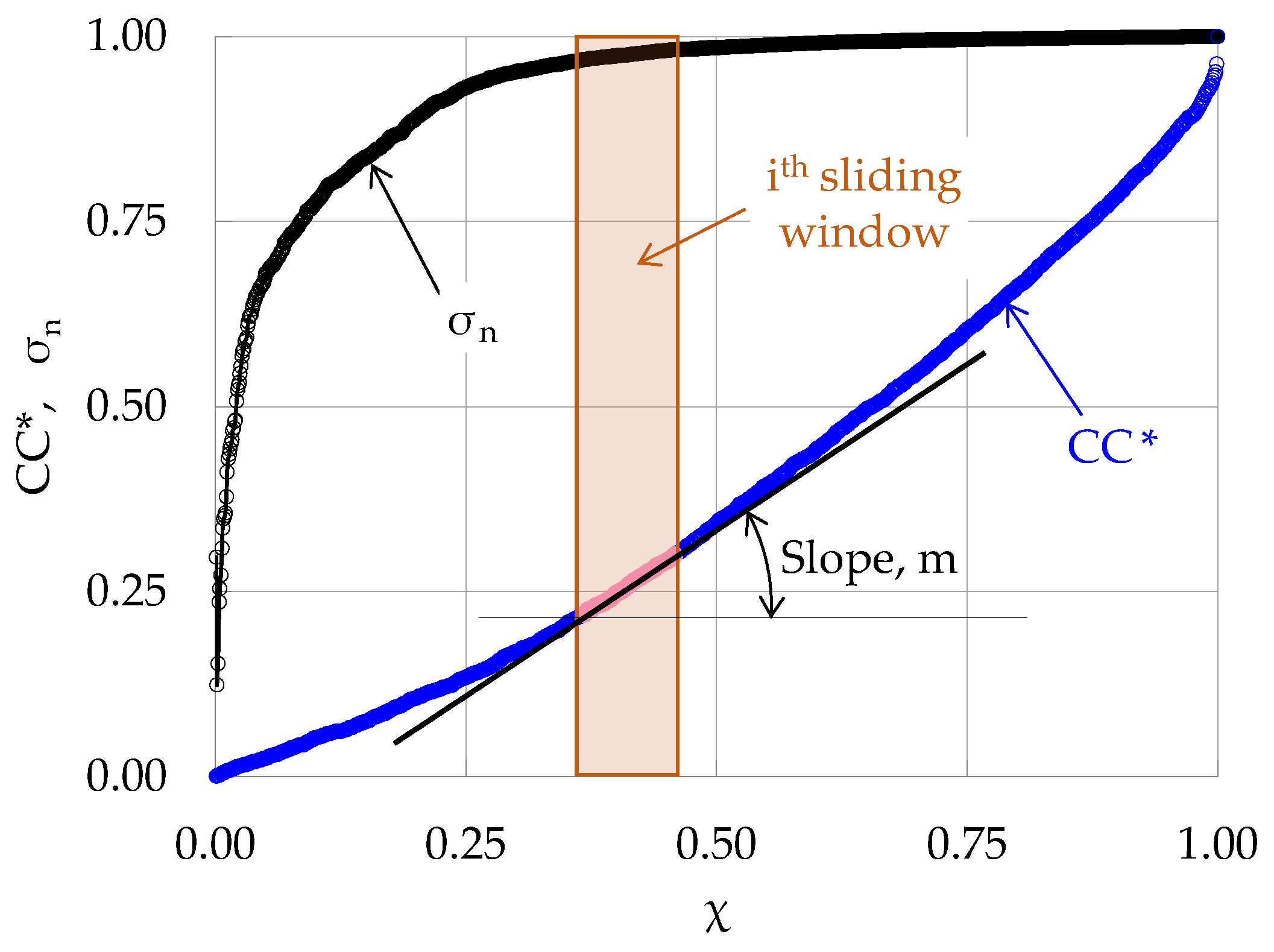
Taking now into account that CC(t) and CC*(t) (and, also, CC*(χ)) are monotonously increasing functions, attention is here paid to the evolution of the respective rate of change in the Natural Time Domain. This is achieved by introducing a parameter m, which quantifies the slope of the linear trendlines corresponding to sub-groups of elements of the time series CC*(χ_k). Each sub-group includes n successive elements. For the needs of this step the “sliding window” procedure is adopted. The main features of this procedure are schematically described in Figure 1. In this figure the evolution of the normalized Cumulative Counts CC* (i.e., of the function CC*(χ)) is plotted (for a typical experiment of the present protocol) versus Natural Time, χ. In the same figure the respective evolution of the externally applied stress (normalized over the maximum value attained) σ_n is, also, plotted.As it can be seen in Figure 1, a sub-group of n elements (denoted as ith sliding window) of the time series (the ones included in the colored rectangle) is isolated and its slope m with respect to χ is calculated by fitting a linear trendline to the n (CC*(χ), χ) pairs of the sub-group under study. The specific value of the slope m is paired to the average value, $\overline{\mathrm{\chi }}$, of the Natural Times of the n elements of the specific group. In this way, a pair (m, $\overline{\mathrm{\chi }}$) is formed. “Sliding” the sub-group by an arbitrary step Δn (in this study the sliding step was set equal to Δn = n/2) a new group is formed, new values for m and $\overline{\mathrm{\chi }}$ are determined, a new pair (m, $\overline{\mathrm{\chi }}$) is formed, and so on. At the end of the specific procedure, a number of (m, $\overline{\mathrm{\chi }}$) pairs is determined, rendering it possible to plot the function m = m($\overline{\mathrm{\chi }}$). For each sub-group of elements, an average value of the applied stress, $\overline{\mathsf{\sigma }}$, is determined equal to the mean value of the stresses corresponding to the n elements of the specific sub-group. Similarly, an average conventional time, $\overline{\mathrm{t}}$, is determined, representing the mean value of the conventional time instants at which the n hits of the sub-group were recorded.

It is mentioned at this point that the choice of the value of n (which governs the “resolution” of the analysis that will be achieved) is somehow subjective. In fact, it is not advised to assign to n a predefined numerical value. As it was concluded in ref. [28], the choice depends mainly on the overall number of acoustic signals recorded during the specific experiment that is analyzed: The greater the overall number of signals, the higher the value of n that can be adopted without significantly shadowing critical details of the analysis. It was proven in that study that the numerical value assigned to n does not significantly influence the results of the analysis (as long as n remains a relatively small fraction of the total number of hits recorded). This conclusion was supported by the analysis of the data of specific experiments, by assigning to n three different numerical values. It was highlighted that the respective plots were extremely close to each other and the main difference between them was the intensity of local fluctuations: increasing the value of n resulted in smoother curves while decreased n-values resulted in somewhat stronger fluctuations. Empirically it can be said that a value equal to about one tenth of the overall number of signals is usually an acceptable choice for most experimental protocols.

Complementary to the study of the evolution of the function m = m($\overline{\mathrm{\chi }}$), the evolution of the average rate of the acoustic hits will be, also, studied, taking advantage of the same sub-groups (“windows”) that were used to determine the numerical values of the parameter m. In this direction, for each one of the “windows” the average rate, $\overline{\mathrm{F}}$, of the acoustic hits is determined as follows [28]:

$$\overline{\mathrm{F} }= {\displaystyle \frac{1 }{\overline{{\mathsf{\delta }\mathsf{\tau }}_{\mathrm{i}}}}}$$

(4)

where $\overline{{\mathsf{\delta }\mathsf{\tau }}_{\mathrm{i}}}$ is the mean value of the interevent time intervals between any two consecutive acoustic hits of each “window”. As previously, each value of $\overline{\mathrm{F}}$, is then paired to the respective average value $\overline{\mathrm{\chi }}$ of the Natural Times of all the elements of the specific group. In this way, ($\overline{\mathrm{F}}$, $\overline{\mathrm{\chi }}$) pairs are formatted, rendering it possible to draw the plot of the respective $\overline{\mathrm{F}}$ = $\overline{\mathrm{F}}$($\overline{\mathrm{\chi }}$) function.

The methodology described in this section has been applied in a very recent publication by the authors’ team [7], in which the function m = m($\overline{\mathrm{\chi }}$) was determined from acoustic data recorded during the experiments of a protocol with notched prismatic beams (made of either plain or fiber-reinforced concrete) submitted to displacement-controlled three-point bending. The main conclusion drawn was that the rate of change of the Cumulative Counts in the Natural Time Domain, i.e., the function m = m($\overline{\mathrm{\chi }}$), provides clearly distinguishable signals warning about the entrance of the loaded system (concrete beams) into the critical stage of impending fracture.

2.2. The Material and the Experimental Protocol

Prismatic specimens of square cross section (45 mm × 45 mm) and length equal to 90 mm were submitted to uniaxial compression. The experiments were realized adopting load-controlled conditions under four different rates equal to 34, 95, 145, and 350 kPa/s. Three experiments were carried out for each loading rate. The specimens of the protocol were made of Dionysos marble, a very fine variety of an almost white marble that is quarried from mount Dionysos in the Attica region of Greece. Given that its properties (both physical and mechanical) are almost identical to the respective ones of Pendelikon marble, the building stone of the Athenian Acropolis monuments, Dionysos marble is the material used to cover the needs of the restoration project of the Parthenon Temple. As a result, its properties are well documented in the respective literature [29,30,31,32]. From the Strength of Materials point of view, it is characterized as an orthotropic material; however, it is usually modeled as transversely isotropic [33,34]. Due to its anisotropic nature (and also, due to the fact that for rocks and rock-like materials, the exact quarrying point and depth influence critically their mechanical response), the numerical values of its mechanical properties vary in a relatively broad interval. Therefore, it is of utmost importance to determine the main properties of each specific block by means of a preliminary experimental protocol rather than to adopt numerical values from the literature.

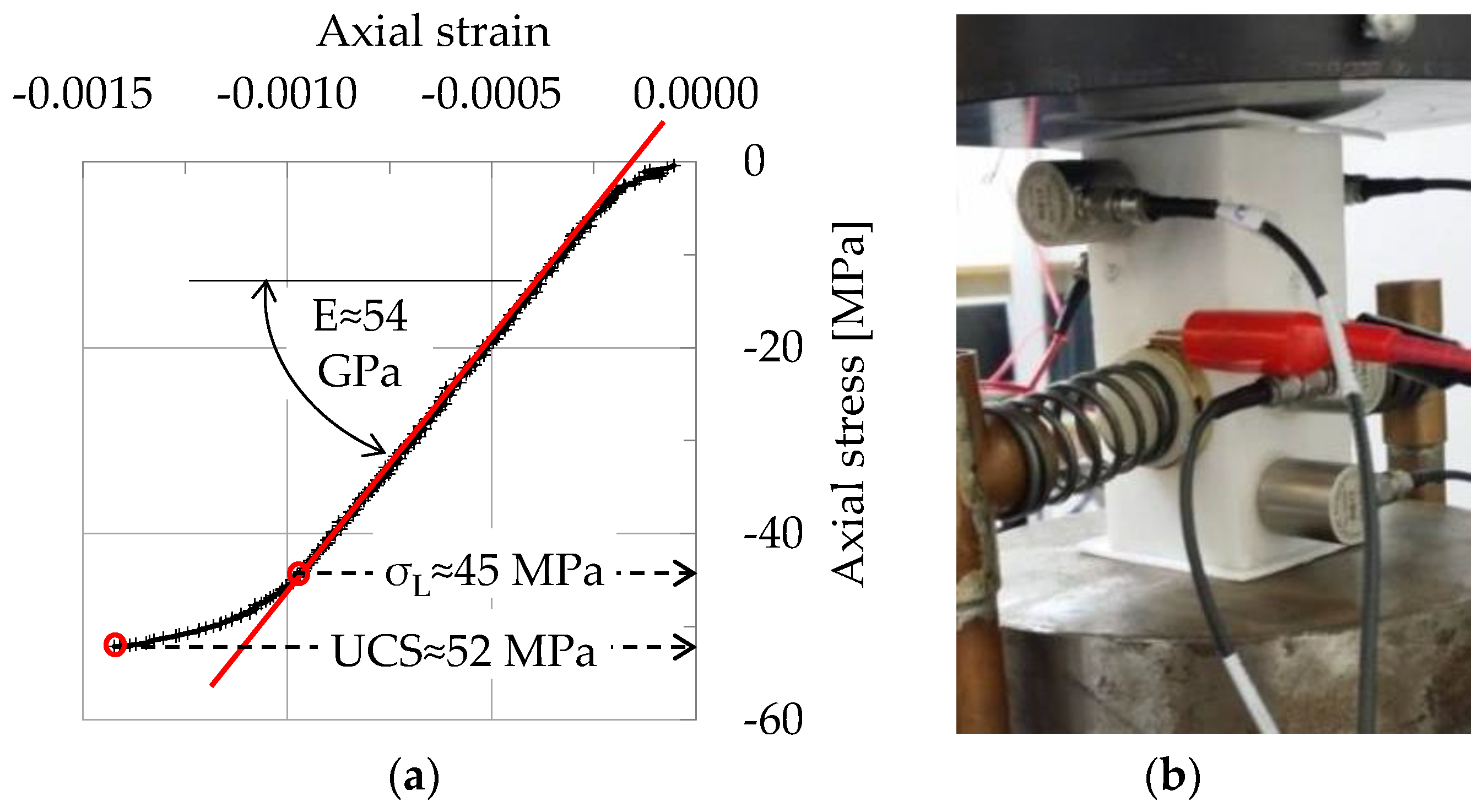
In this context, the results of a typical experiment from the preliminary protocol which was implemented for the needs of the present study, are shown in Figure 2a, in which the axial stress applied is plotted versus the respective axial strain developed. It was concluded from this preliminary protocol that the response of the specific block of Dionysos marble (i.e., the block from which the specimens of the main protocol were cut) is characterized by an extensive linear elastic regime of the stress–strain plot, ranging from about 7 MPa to about 45 MPa, or, equivalently, from about 13% to about 87% of its compressive strength. The latter varies around 52 MPa. The modulus of elasticity was determined equal to about 54 GPa.

The acoustic activity was recorded using R15a sensors (Figure 2b). The gain of the preamplifier of the experimental set-up was equal to 40 dB and the cut-off threshold was set to 40 dB, taking advantage of experience gained from previous protocols with marble specimens. The software and hardware used were by Mistras Group, Inc., Princeton Junction, NJ, USA. The scattering between experiments with specimens loaded under the same loading rate were insignificant. Therefore, data from only four characteristic experiments (one for each loading rate) will be thoroughly analyzed in next sections.

3. Results

3.1. The Rate of Change, m, of the Cumulative Counts in the Natural Time Domain, χ

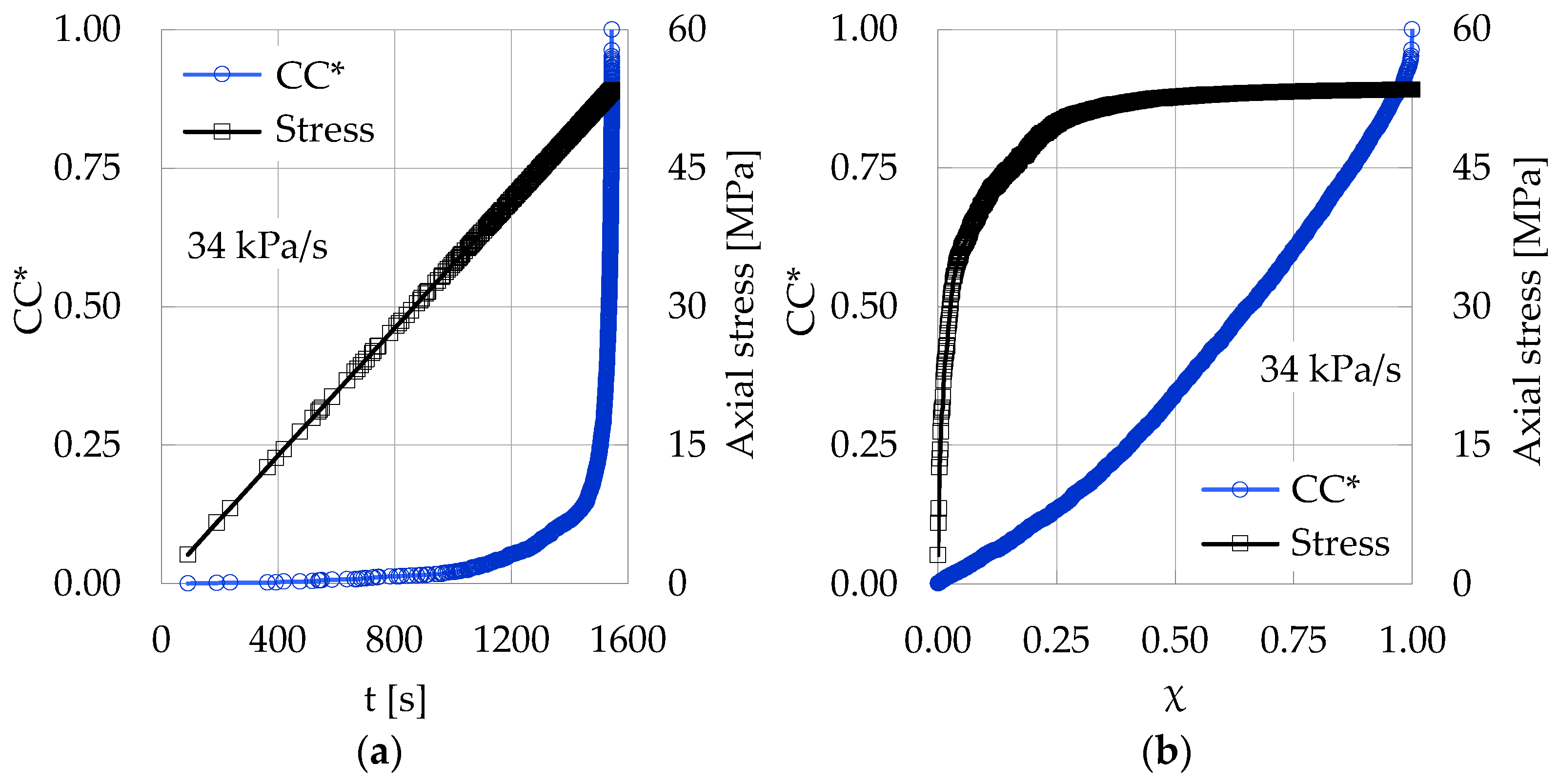
As a first step, the procedure for analyzing experimental data according to the methodology introduced here is thoroughly described for a typical specimen of the class loaded under the lowest rate, i.e., 34 kPa/s. For the specific experiment the fracture stress was equal to 53.5 MPa, and the overall number of acoustic hits that were recorded was equal to N = 1079. The evolution of the normalized Cumulative Counts (CC*) in terms of the conventional time, t, is plotted in Figure 3a, while the respective evolution in terms of the Natural Time, χ, is plotted in Figure 3b.

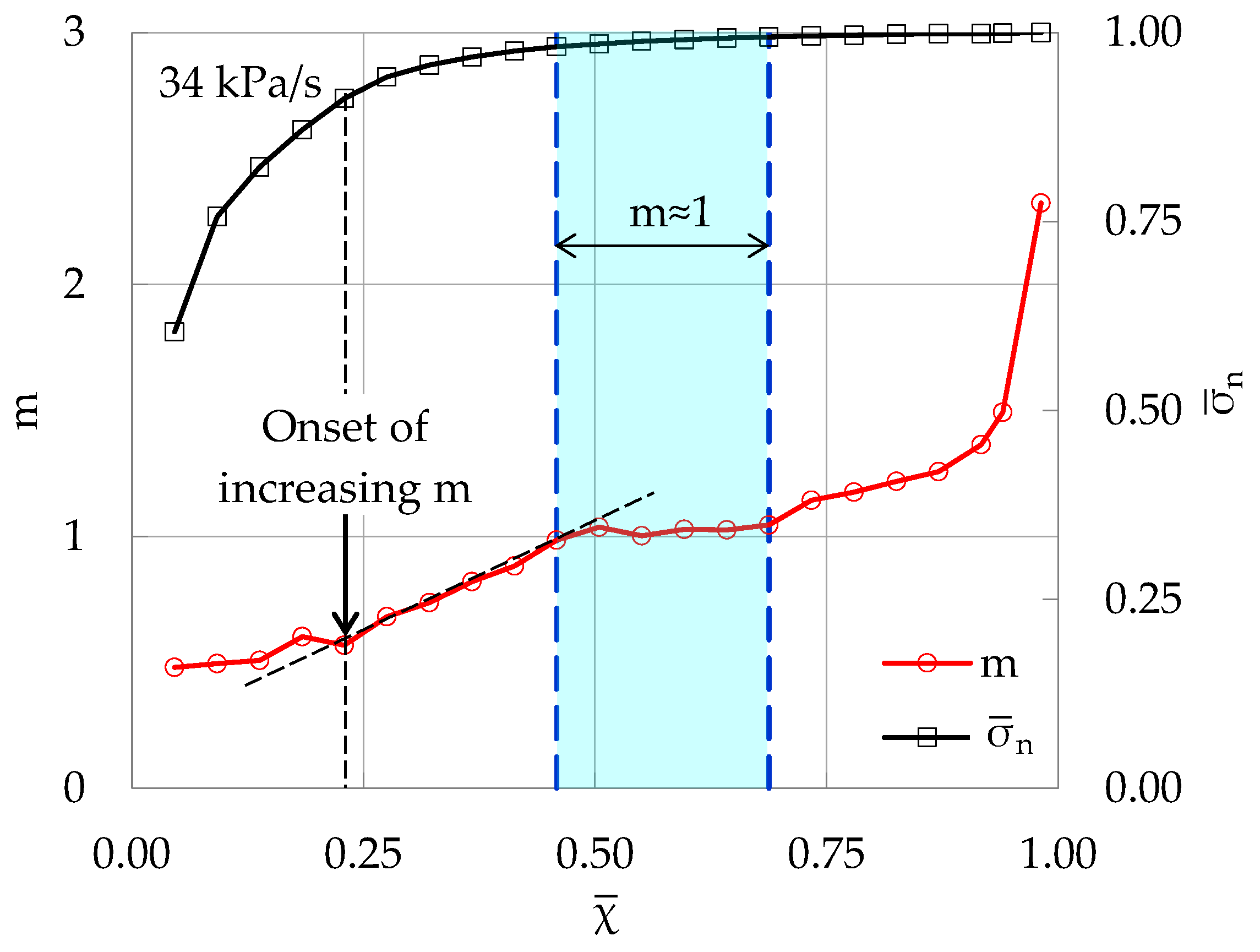
Adopting then the “sliding window” technique (described synoptically in Section 2.1), the rate m of change of CC*(χ) (i.e., the slope of the CC*(χ) function) is calculated. In this context, sub-groups containing n = 100 successive hits are considered with a “sliding step” equal to Δn = n/2 = 50 hits. Pairing each m-value to the mean value, $\overline{\mathrm{\chi }}$, of the Natural Times, χ_i, of all the n elements of the specific sub-group, the function m = m($\overline{\mathrm{\chi }}$) is structured and is plotted in Figure 4.

In the same figure the respective evolution of the average applied stress, ${\overline{\mathsf{\sigma }}}_n$ is also plotted. The latter is calculated as the mean value of the stresses corresponding to each one of the n acoustic hits of the sub-group studied and is normalized over the maximum stress attained (i.e., over the compressive strength of each specimen).

It is observed from Figure 4 that the values of m start increasing, almost linearly, at a Natural Time “instant” $\overline{\mathrm{\chi }}$ ≈ 0.23, while the stress attains a value equal to ${\overline{\mathsf{\sigma }}}_n \approx 0.91$(i.e., at about 91% of the maximum stress applied during the specific experiment). However, the most intriguing characteristic of Figure 4 is that at the instant $\overline{\mathrm{\chi }}$ ≈ 0.46 (corresponding to a normalized stress level equal to ${\overline{\mathsf{\sigma }}}_n \approx 0.981$) the values of the m attain a plateau with m ≈ 1. The duration of this plateau is Δt ≈ 20 s, or, in terms of the Natural Time it covers the interval 0.46 < $\overline{\mathrm{\chi }}$ < 0.69. Alternatively, in terms of the normalized stress, it covers the interval $0.981 \le {\overline{\mathsf{\sigma }}}_{n }\le 0.994$. After this plateau, m starts increasing again for about 9 s, until the macroscopic fracture of the specimen, suggesting that at this stage the acoustic hits recorded are associated with an increased number of counts due to the impending propagation of fatal macro-cracks. Based on the above observations, it could be argued that the plateau of the m-values, signals the entry of the loaded system into the critical stage of impending fracture, or, in others words, to the transitional stage from generation of micro-cracks to that of the coalescence of them in the direction of forming the fatal macro-crack.

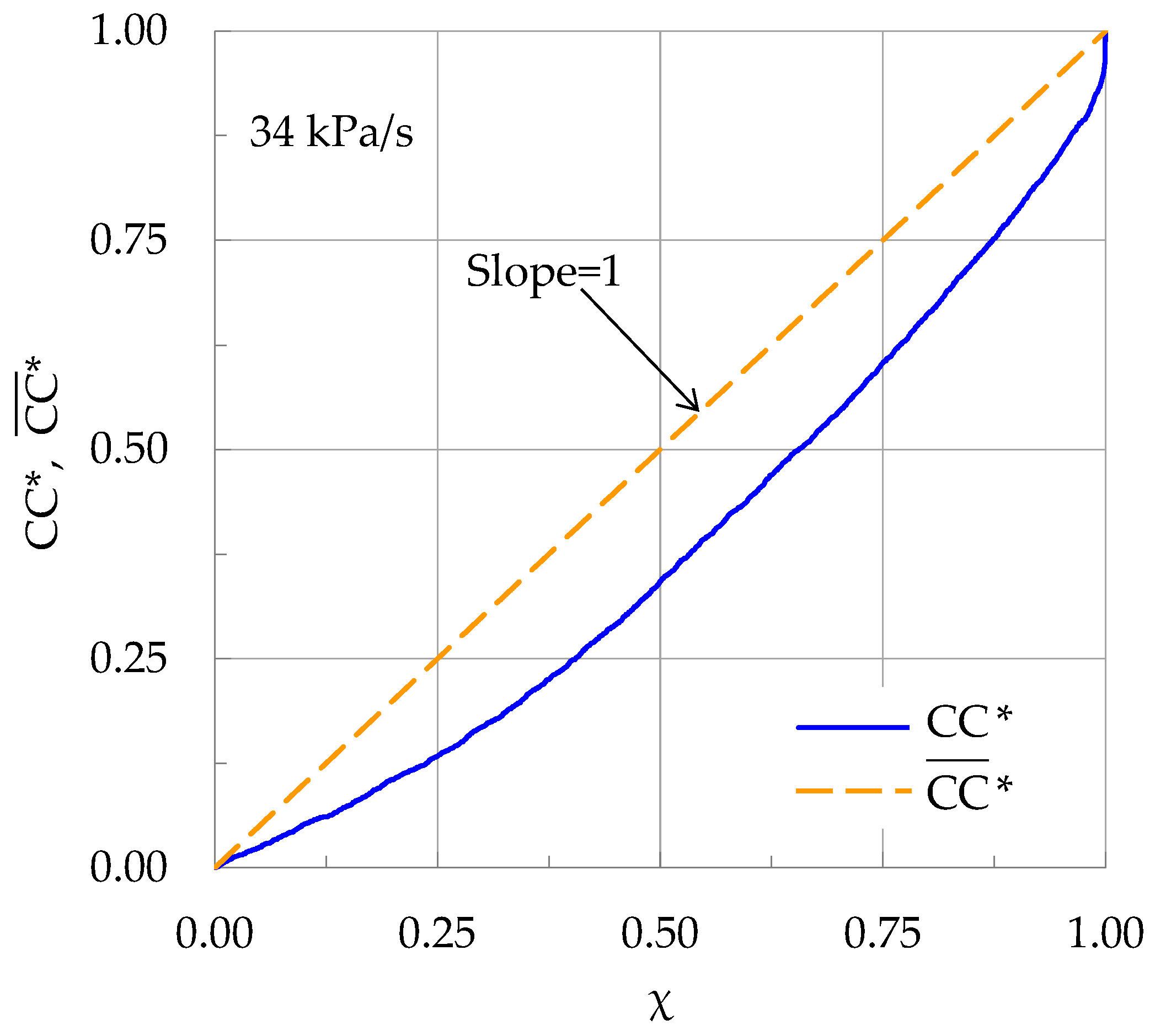
From an alternative point of view, the value m = 1 corresponds to the constant slope of a function CC*(χ) for a fictitious experiment with all its acoustic hits having exactly the same number of counts. Such a function is plotted by dashed straight line in Figure 5, assuming that all the acoustic hits have the same number of counts, equal to the mean value of the counts of all the hits of the specific experiment (i.e., that loaded at a rate of 34 kPa/s) discussed here (see Figure 3). In the same figure, the actual CC*(χ) function corresponding to the specific experiment is plotted for comparison. Obviously, at stages of the loading procedure with m equal to—or higher than—the m ≈ 1 threshold, acoustic signals characterized by increased number of counts prevail, or equivalently, acoustic signals characterized by increased energy content. However, it is known (see, for, example, refs. [1,8,9,35]), that acoustic signals with increased energy content prevail during the critical stages of impending fracture. In this context, the plateau with m ≈ 1 could be considered as an additional indicator that “strong” signals are produced, warning, thus, about upcoming disastrous fracture.

3.2. The Influence of the Loading Rate on the Rate of Change, m, of the Cumulative Counts in the Natural Time Domain, χ

In an attempt to explore the potential role of the loading rate on the conclusions drawn in the previous section (and especially on the conclusions regarding the possibility that the plateau m ≈ 1 of the evolution of m in the Natural Time Domain could be a pre-failure indicator) additional experiments were implemented with stress rates equal to 95, 145 and 350 kPa/s (i.e., up to ten times higher compared to the experiments discussed in Section 3.1). Again, one experiment for each loading rate will be thoroughly analyzed (taking into account that the scattering of the results between experiments of the same class were almost insignificant).

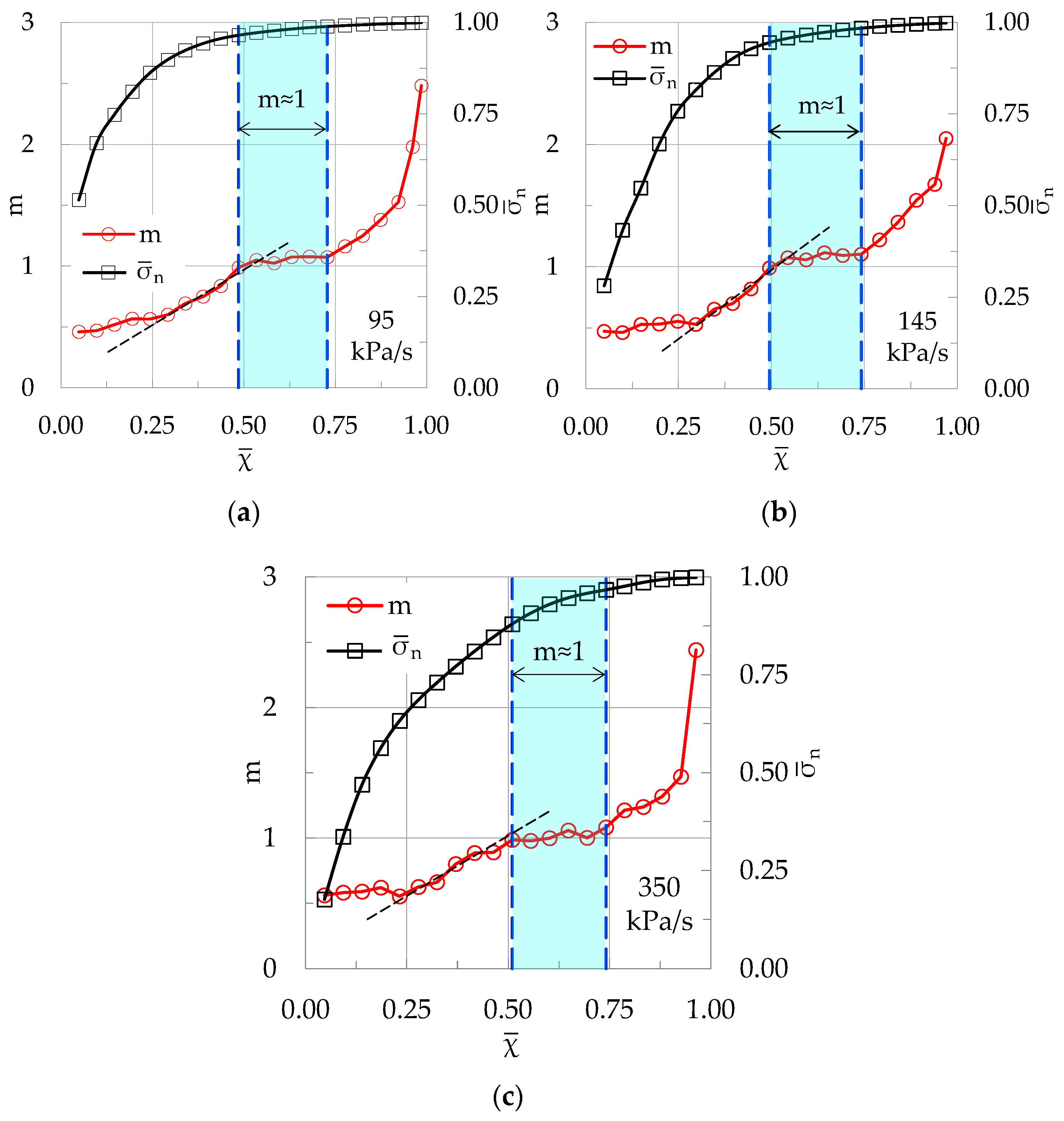
For these characteristic experiments the fracture stress of the specimens tested was equal to 52.2, 52.3, and 50.7 MPa for the rates of 95, 145, and 350 kPa/s, respectively. The overall number of acoustic hits recorded during the above experiments was equal to 1031, 1012 and 1080, respectively. Since these numbers are quite similar to that of the experiment discussed in Section 3.1 (N = 1079), the same “sliding window” of n = 100 successive acoustic hits was adopted (with the same “sliding step” of Δn = n/2 = 50 hits) for the determination of the function m = m($\overline{\mathrm{\chi }}$). The evolution of m versus the average Natural Time $\overline{\mathrm{\chi }}$ is plotted in Figure 6a–c) for all three loading rates. In the same figures, the corresponding average applied stress, ${\overline{\mathsf{\sigma }}}_n$, is also plotted.

The qualitative similarities between the three experiments of Figure 6 (and, also, with the experiment of Section 3.1, i.e., the one at which the specimen was loaded at a rate of 34 kPa/s), regarding the evolution of the rate m of change of the normalized Cumulative Counts (CC*) in terms of the Natural Time, χ, are obvious: Independently of the loading rate imposed, the values of m increase gradually until the plateau with m ≈ 1 is attained. They are stabilized for an interval of χ-values and then, they start increasing again until the fracture of the specimen. What is different, depending on the loading rate, is the extent (duration) of the plateau, both in terms of conventional time, and also, in terms of the average normalized applied stress, ${\overline{\mathsf{\sigma }}}_{\mathrm{n}}$.

These differences are quantified in

Table 1. The starting and terminal “instants” of the plateau with m ≈ 1 and its duration in terms of stress and conventional time. The duration of the stage with m > 1 is, also, shown together with the UCS and the overall duration of each experiment.

σR [kPa/s]	σmax [MPa]	tf [s]	Stage with m ≈ 1				Stage with m > 1
			${\overline{\mathsf{\sigma }}}_{\mathbf{n}\mathbf{,}\mathbf{s}}$	${\overline{\mathsf{\sigma }}}_{\mathbf{n}\mathbf{,}\mathbf{e}}$	(Δ${\overline{\mathsf{\sigma }}}_{\mathbf{n}}$)m≈1	(Δt)m≈1	(Δt)m>1
34	53.5	1545	0.981	0.994	0.013	20.1	9.3
95	52.2	549.2	0.965	0.989	0.024	13.2	6.0
145	52.3	360.8	0.945	0.984	0.039	14.1	5.8
350	50.7	145.3	0.881	0.967	0.087	12.5	4.8

, in which the values of the normalized applied stress at the starting and at the terminal points of the plateau, denoted as ${\overline{\mathsf{\sigma }}}_{\mathrm{n},\mathrm{s}}$ and ${\overline{\mathsf{\sigma }}}_{\mathrm{n},\mathrm{e}}$, respectively, are shown, together with the duration of the plateau, both in terms of stress, $(\Delta {\overline{\mathsf{\sigma }}}_{\mathrm{n}}{)}_{\mathrm{m}\approx 1} ={\overline{ \mathsf{\sigma }}}_{\mathrm{n},\mathrm{e}} - {\overline{\mathsf{\sigma }}}_{\mathrm{n},\mathrm{s}}$, and also, in terms of the conventional time, (Δt)_m≈1. In addition, the duration, (Δt)_m>1 of the stage with m > 1 is recorded for each experiment. For completeness reasons, the maximum stress attained, σ_max, and the overall duration (t_f) of each experiment (from the onset of loading up to the fracture of each specimen) are also recorded for all four stress rates, σ_R, of the protocol.

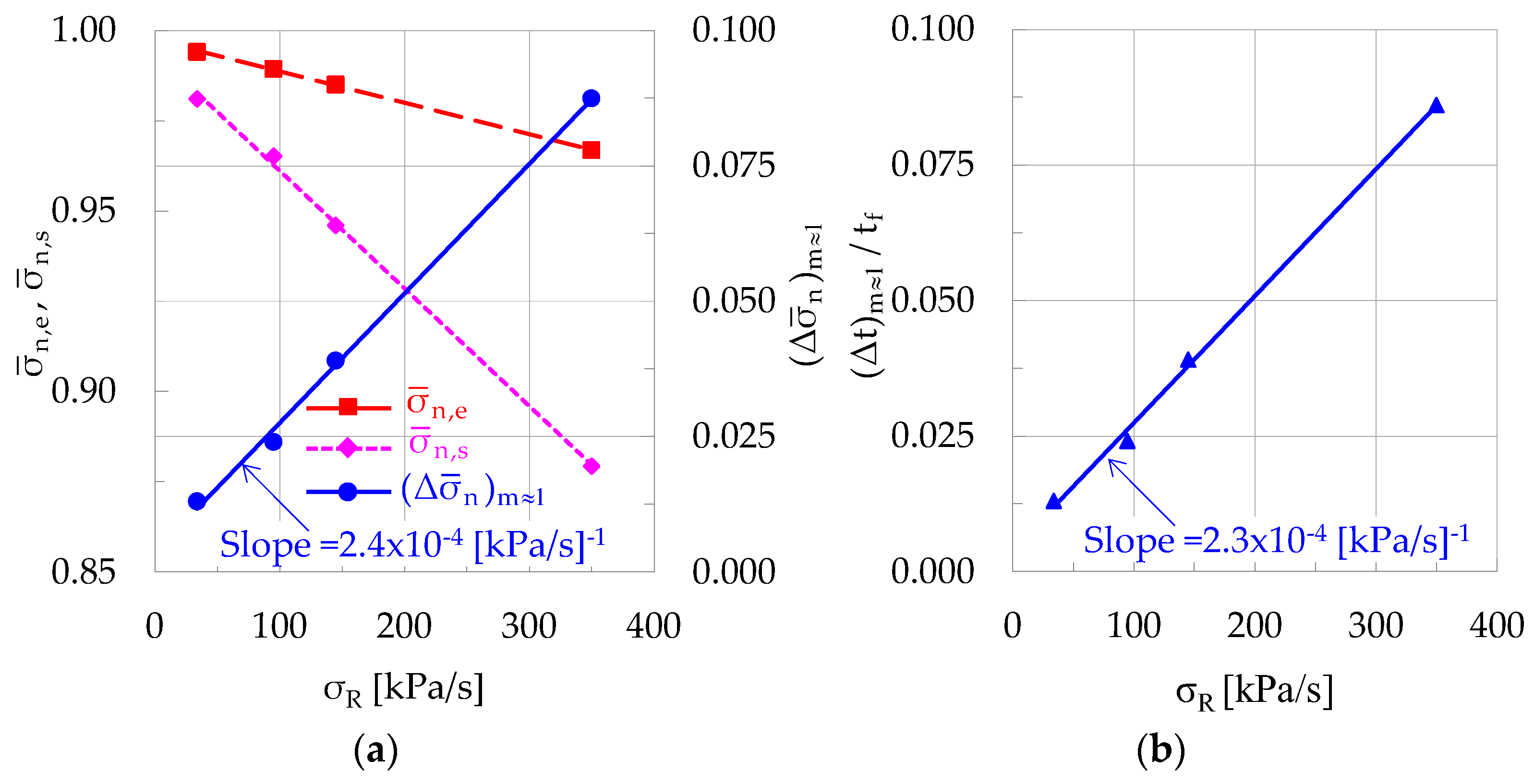
Now paying attention to the limits of the plateau (i.e., the interval with m ≈ 1), in terms of the average normalized stress, a linear decrease in both the starting and the terminal “instants”, ${\overline{\mathsf{\sigma }}}_{\mathrm{n},\mathrm{s}}$ and ${\overline{\mathsf{\sigma }}}_{\mathrm{n},\mathrm{e}}$, respectively, is observed with increasing loading rate, as it can be seen in Figure 7a. Especially the decrease in ${\overline{\mathsf{\sigma }}}_{\mathrm{n},\mathrm{s}}$ implies tacitly that increased loading rates “translate” the critical stage of impending fracture (at least as it is heralded by the onset of the m ≈ 1 plateau) at earlier loading levels. For example, it is mentioned characteristically that for the experiment with the highest loading rate (i.e., σ_R = 350 kPa/s), the m = 1 stage appears almost simultaneously with the onset of the non-linear stress-strain response of the specimen, i.e., the “instant”, ${\overline{\mathsf{\sigma }}}_{\mathrm{n},\mathrm{s}}$ ≈ 0.88. Another interesting observation is that the decrease in the starting “instant”, ${\overline{\mathsf{\sigma }}}_{\mathrm{n},\mathrm{s}}$, is much more rapid compared to that of the terminal one, and ${\overline{\mathsf{\sigma }}}_{\mathrm{n},\mathrm{e}}$. As a result, the “duration” of the plateau, ${\left(\Delta {\overline{\mathsf{\sigma }}}_{\mathrm{n}}\right)}_{\mathrm{m}\approx 1} = {\overline{\mathsf{\sigma }}}_{\mathrm{n},\mathrm{e}}-{\overline{\mathsf{\sigma }}}_{\mathrm{n},\mathrm{s}}$, increases significantly with increasing loading rate, as it can be seen in Figure 7a.

In order now to comparatively study the duration of the m ≈ 1 plateau in terms of the conventional time, t, it is imperative to take into account that the overall duration, t_f, of each experiment does obviously depend straightforwardly on the loading rate (by increasing the loading rate the overall duration of the experiment decreases). In this context, considering that for all experiments the loading rate was kept constant during the overall duration of the loading procedure, and also, that no significant time elapses between the macroscopic fracture and the maximization of the applied load (there is not a stage of decreasing load in the present experimental protocol), it can be written as:

$${\displaystyle \frac{\left(\Delta {\mathsf{\sigma }}_{\mathrm{n}}\right)}{\Delta \mathrm{t}}}={\displaystyle \frac{1}{{\mathrm{t}}_{\mathrm{f}}}}$$

(5)

In addition, it holds that:

$${\displaystyle \frac{{(\Delta \mathrm{t})}_{\mathrm{m}\approx 1}}{{\mathrm{t}}_{\mathrm{f}}}}={\left(\Delta {\overline{\mathsf{\sigma }}}_{\mathrm{n}}\right)}_{\mathrm{m}\approx 1}$$

(6)

or, in other words, the normalized duration (Δt)_m≈1/t_f of any experiment (in terms of conventional time, t) is almost identical to the respective width (“duration”) in terms of the average applied stress, ${\left(\Delta {\overline{\mathsf{\sigma }}}_{\mathrm{n}}\right)}_{\mathrm{m}\approx 1}$. This is clearly seen, also, from Figure 7b in which the duration (Δt)_m≈1/t_f of the m ≈ 1 plateau is plotted versus the loading rate: it is evident that the slope of the specific plot is practically identical to the respective one of ${\left(\Delta {\overline{\mathsf{\sigma }}}_{\mathrm{n}}\right)}_{\mathrm{m}\approx 1}$ derived from Figure 7a.

Recapitulating about the data concerning the role of the loading rate, it can be said that while at the highest one (350 kPa/s), the stress threshold ${\overline{\mathsf{\sigma }}}_{\mathrm{n},\mathrm{s}}$ for the appearance of the m ≈ 1 plateau is only 0.881, it increases linearly to 0.981 for the lowest loading rate of 34 kPa/s. The physical basis of this dependence deserves to be further studied from the perspective of Fracture Mechanics for a broader variety of materials and loading schemes.

3.3. The Evolution of the Average Rate of Production of Acoustic Hits in the Natural Time Domain

As a next step, and in order to compare the outcomes of the present analysis regarding the evolution of m with the respective ones of alternative approaches, the rate of generation of acoustic signals will be analyzed, also, in the Natural Time Domain. The same procedure adopted for the determination of m (i.e., “sliding windows” with sub-groups of n = 100 successive elements and a “sliding step” of Δn = n/2 = 50) will also be used for the determination of the average rate $\overline{\mathrm{F}}$ of generation of acoustic hits.

In this context, and taking advantage of Equation (4), the numerical value of $\overline{\mathrm{F}}$ is determined for each sub-group and is, then, paired to the average value, $\overline{\mathrm{\chi }}$, of the n values of the Natural Times, χ_i, corresponding to each one of the n elements of the specific sub-group. In addition, the respective average value of the conventional time instants, $\overline{\mathrm{t}}$, and the average value of the normalized applied stress, ${\overline{\mathsf{\sigma }}}_{\mathrm{n}},$ are calculated for each sub-group. As a first application, the experiment with loading rate equal to 34 kPa/s is analyzed here.

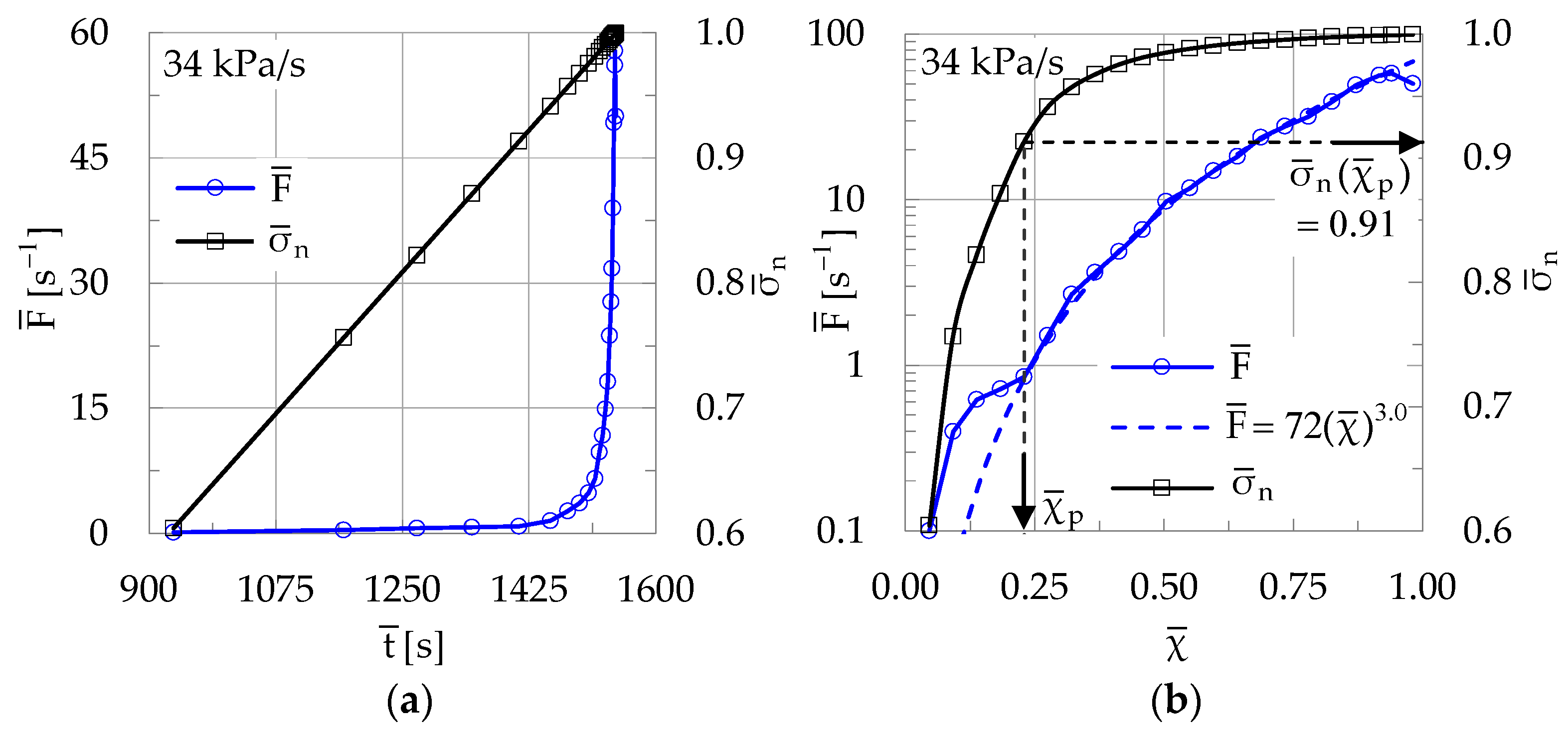
The evolution of $\overline{\mathrm{F}}$, is plotted in Figure 8a versus the average conventional time, $\overline{\mathrm{t}}$, and in Figure 8b versus the average Natural Time, $\overline{\mathrm{\chi }}$. In both figures, the respective evolution of the normalized average stress applied, ${\overline{\mathsf{\sigma }}}_{\mathrm{n}}$, is also plotted. It is seen from Figure 8a that a quite abrupt increase in $\overline{\mathrm{F}}$ towards a global maximum ${\overline{\mathrm{F}}}_{\max }$ is observed a few seconds before the instant of macroscopic fracture, indicating a very strongly accelerated rate of production of acoustic signals, in full accordance with similar findings deduced from experimental protocols with specimens made of a broad variety of materials [10,13,21,36].

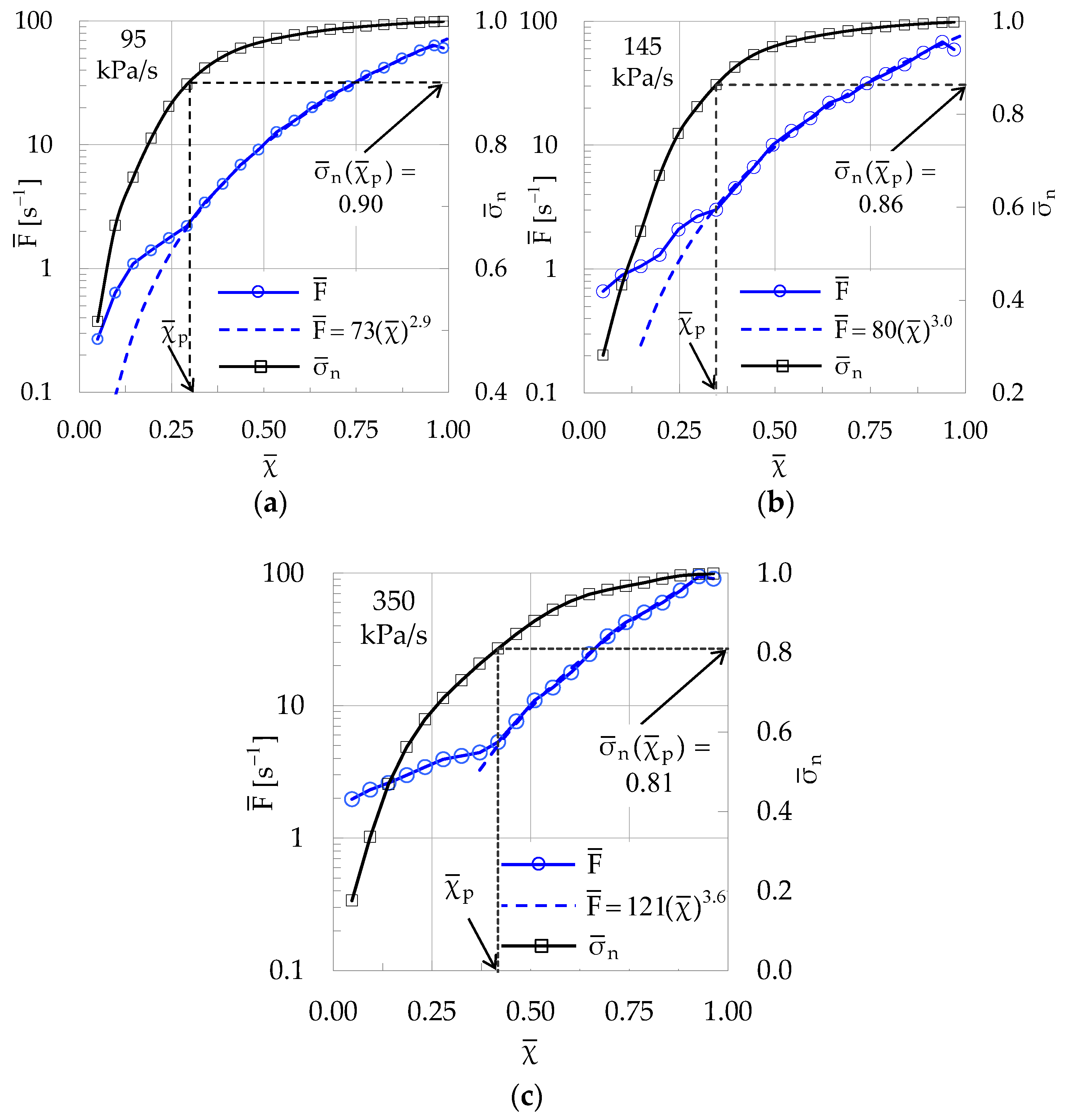
On the other hand, the evolution of $\overline{\mathrm{F}}$, in the Natural Time Domain (Figure 8b), is completely different. There is a clear threshold, ${\overline{\mathrm{\chi }}}_{\mathrm{P}}$ = 0.23, which corresponds to an average stress threshold ${\overline{\mathsf{\sigma }}}_{\mathrm{n}}\left({\overline{\mathrm{\chi }}}_{\mathrm{P}}\right)$ = 0.913, beyond which the evolution of the function $\overline{\mathrm{F}}\left(\overline{\mathrm{\chi }}\right)$ is governed by a power law of the following form:

$$\overline{\mathrm{F}}\left(\overline{\mathrm{\chi }}\right) ={ \mathrm{A} \overline{\mathrm{\chi }} }^{\mathrm{k}}$$

(7)

The law of Equation (7) dictates the evolution of the function $\overline{\mathrm{F}}\left(\overline{\mathrm{\chi }}\right)$ up to the penultimate “sliding window” (sub-group), at which $\overline{\mathrm{F}}\left(\overline{\mathrm{\chi }}\right)$ attains its maximum value ${\overline{\mathrm{F}}}_{\max }$. During the last “window”, the duration of which is only 0.8 s, a slight decrease in the value of $\overline{\mathrm{F}}\left(\overline{\mathrm{\chi }}\right)$ is observed. This decrease has been highlighted systematically in many protocols and has been critically commented in ref. [28]. It is mainly attributed to the fact that at this very last stage of the loading procedure, a few long-duration acoustic hits are typically recorded; consequently, the inter-event times are longer. As a result, the function $\overline{\mathrm{F}}\left(\overline{\mathrm{\chi }}\right)$ exhibits inevitably a decreasing trend. In addition, at this stage, the macro-crack has been formed and starts propagating, consuming large amounts of the elastic strain energy, which is stored within the bulk of the loaded specimen. Therefore, there is no longer sufficient strain energy that could maintain an increased rate of generation of additional microcracks or, equivalently, to maintain the increasing trend of the function $\overline{\mathrm{F}}\left(\overline{\mathrm{\chi }}\right)$.

The power law of Equation (7) governs the response of a variety of materials under various loading protocols, independently of the specimens’ geometry. For example, both notched and intact beams made of either plain or fiber-reinforced concrete were studied in ref. [10] and it was concluded that the power law of Equation (7) was valid in all cases. Similar conclusions about the validity of the specific law were drawn from a series of experimental protocols with marble specimens under a variety of loading schemes as it is described in ref. [37].

The respective results for the specimens loaded under increased loading rates, i.e., the rates of 95, 145, and 350 kPa/s, are plotted in Figure 9a, b, and c, respectively.

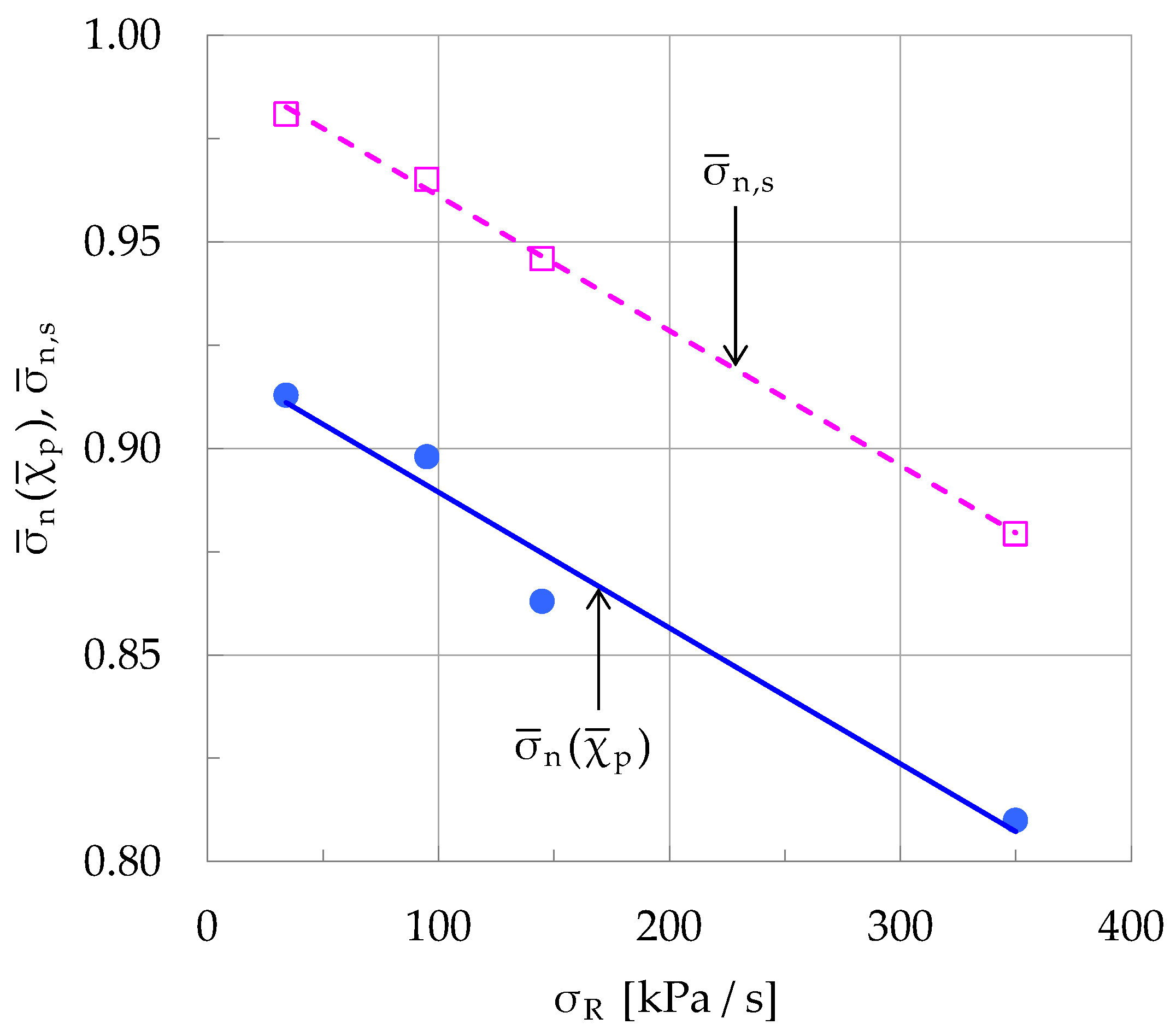
The above numerical data for the ${\overline{\mathsf{\sigma }}}_{\mathrm{n}}\left({\overline{\mathrm{\chi }}}_{\mathrm{p}}\right)$ threshold, are recapitulated in

Table 2. The numerical values of the ${\overline{\mathsf{\sigma }}}_{\mathrm{n}}\left({\overline{\mathrm{\chi }}}_{\mathrm{p}}\right)$ threshold, for each loading rate used in the experimental protocol together with the respective values of the ${\overline{\mathsf{\sigma }}}_{\mathrm{n},\mathrm{s}}$ threshold (designating the onset of the m = 1 plateau—see Section 3.2).

σR	${\overline{\mathsf{\sigma }}}_{\mathbf{n}}\left({\overline{\mathsf{\chi }}}_{\mathbf{p}}\right)$	${\overline{\mathsf{\sigma }}}_{\mathbf{n},\mathbf{s}}$
34	0.913	0.981
95	0.898	0.965
145	0.863	0.945
350	0.810	0.881

together with the respective values of the ${\overline{\mathsf{\sigma }}}_{\mathrm{n},\mathrm{s}}$ threshold, which corresponds to the stress level at which the m ≈ 1 plateau is attained, as it was previously discussed in Section 3.2.

The dependence of the above mentioned two thresholds (i.e., the ${\overline{\mathsf{\sigma }}}_{\mathrm{n}}\left({\overline{\mathrm{\chi }}}_{\mathrm{p}}\right)$ and the ${\overline{\mathsf{\sigma }}}_{\mathrm{n},\mathrm{s}}$ ones) on the loading rate σ_R, is more vividly shown in Figure 10. It is seen from this figure that the ${\overline{\mathsf{\sigma }}}_{\mathrm{n}}\left({\overline{\mathrm{\chi }}}_{\mathrm{p}}\right)$ threshold is systematically lower than the ${\overline{\mathsf{\sigma }}}_{\mathrm{n},\mathrm{s}}$ one. This fact indicates that the onset of the accelerated rate of AE hits occurs at earlier loading stages (lower stress levels), however, the acoustic signals with an increased number of counts do not dominate yet (in other words, m is still lower than the m ≈ 1 limit).

A comparative and thorough consideration of the evolution of the m = $\mathrm{m}(\overline{\mathrm{\chi }})$ function, as it is plotted in Figure 4 and Figure 6, indicates that the numerical values of the ${\overline{\mathsf{\sigma }}}_{\mathrm{n}}\left({\overline{\mathrm{\chi }}}_{\mathrm{p}}\right)$ threshold are very close to the values of the average normalized stress level at which the parameter m starts increasing almost linearly towards the m ≈ 1 limit. Therefore, it could be concluded that as the rate of generation of acoustic signals is accelerated, the average slope of the Cumulative Counts starts increasing due to the generation of hits with increased energy content, or equivalently with increased number of counts. In addition, it is concluded from Figure 10 that the dependence of the ${\overline{\mathsf{\sigma }}}_{\mathrm{n}}\left({\overline{\mathrm{\chi }}}_{\mathrm{p}}\right)$ threshold on the loading rate is almost linear, as it was the case of the ${\overline{\mathsf{\sigma }}}_{\mathrm{n},\mathrm{s}}$ threshold, and, moreover, the slope of the respective plots is almost the same.

4. Discussion

It is interesting to explore now whether the appearance of a stage of the loading procedure during which the values of m are practically stabilized at the m ≈ 1 limit, is systematic (at least for specimens made of marble), independently of the loading scheme and the shape of the specimens. In this direction, advantage will be taken of experimental data from two previously published protocols by the authors’ team, in both of which specimens made of Dionysos marble were tested.

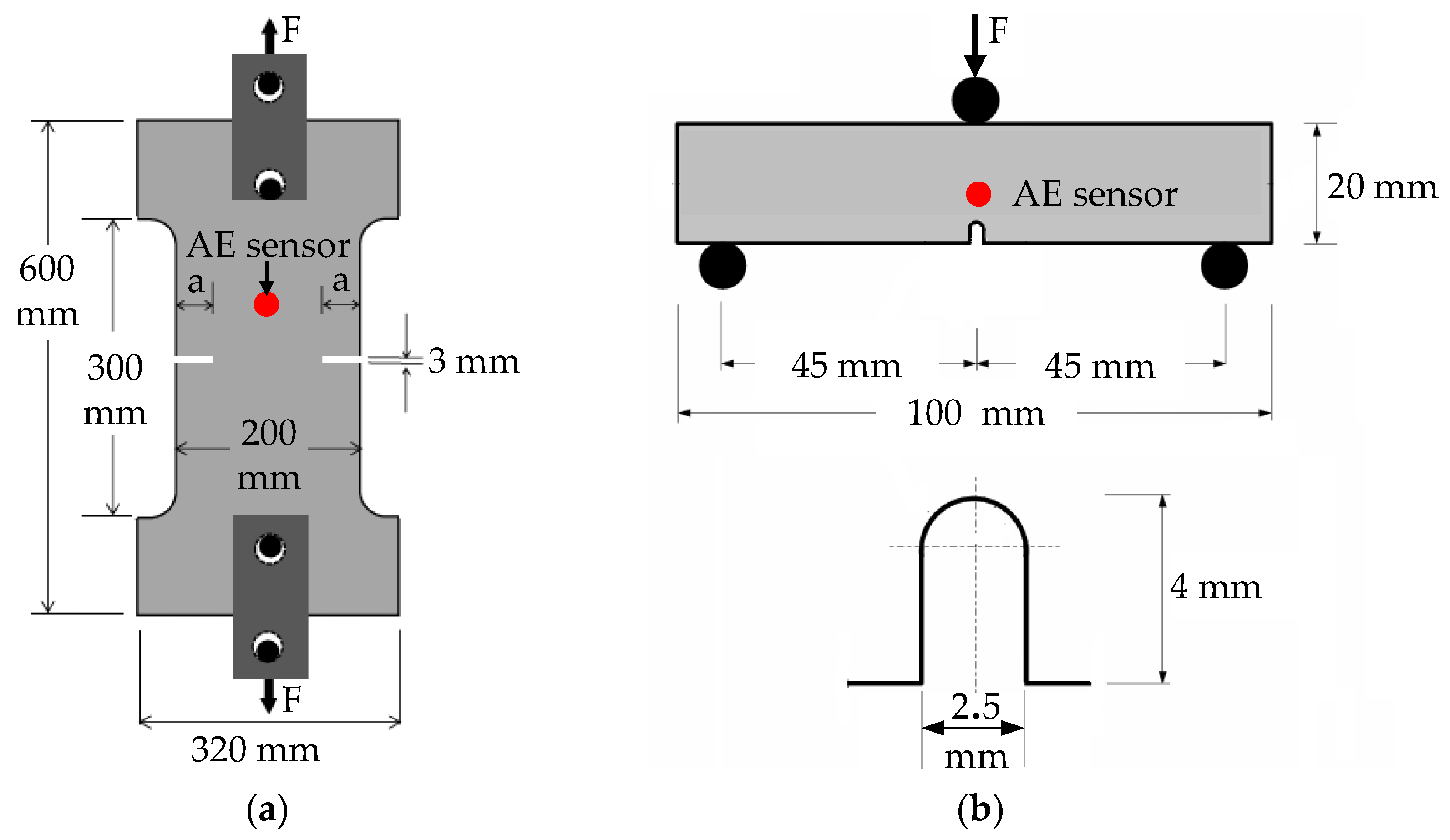
The first protocol refers to direct uniaxial tension of plates shaped in the form of Double Edge Notched (DEN) specimens. The two notches (symmetrically machined with respect to the loading axis) had a length equal to a = 6 cm. The geometry and the dimensions of the specimens are shown in Figure 11a. The second protocol refers to three-point bending (3PB) of notched prismatic beams of square cross-section, the geometry and the dimensions of which can be seen in Figure 11b.

The experiments of both those protocols were carried out under quasi-static conditions, adopting displacement-controlled schemes, at constant rates equal to 0.2 mm/min for the first protocol and 0.01 mm/min for the second one. Further analytical details regarding these two protocols, i.e., the experimental setup, and the AE monitoring and recording system are reported in a previous work by the authors’ team [37], in which the acoustic activity was studied in terms of the time-to-failure parameter, t_f-t, rather than in terms of the Natural Time, χ.

4.1. The Evolution of m and $\overline{F}$ in the Natural Time Domain for the Protocol with DEN Specimens

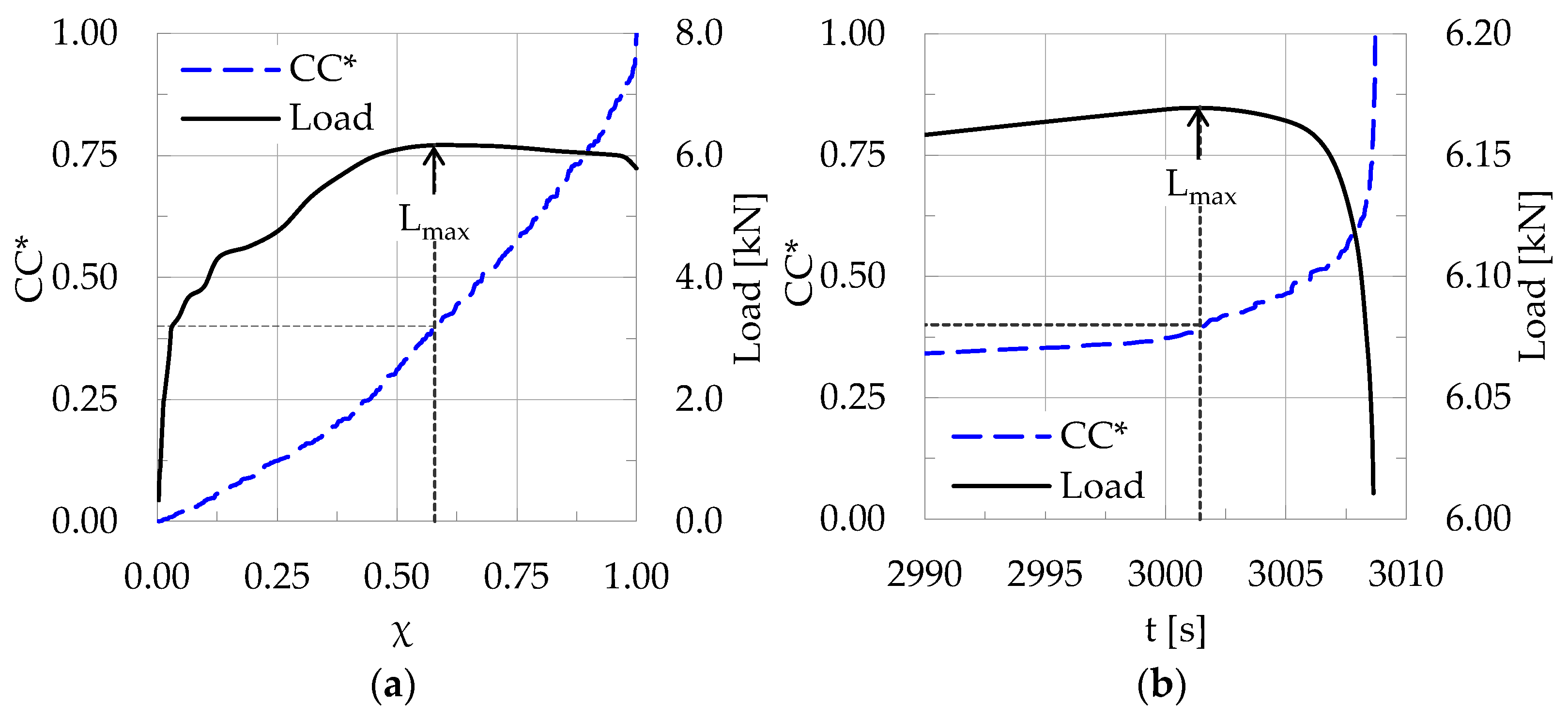
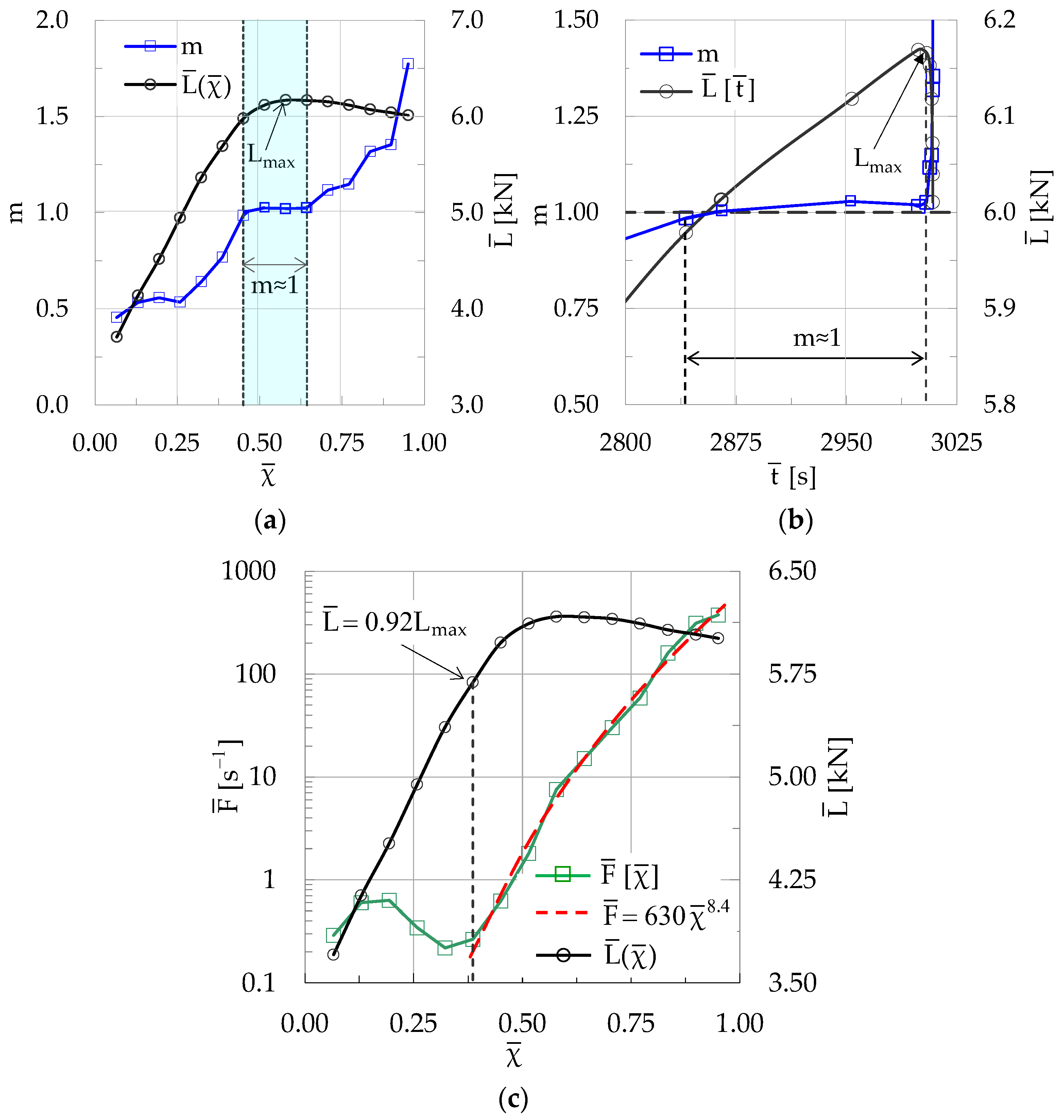
Taking advantage of the data recorded by an acoustic sensor placed in the vicinity of the notches the normalized values of the Cumulative Counts CC*(χ) were determined and were juxtaposed to the respective values of the applied force, denoted from here on as L(χ). The results of this effort are shown in Figure 12a in terms of Natural Time, χ, and in Figure 12b in terms of conventional time, t.

In Figure 12b only the last loading stage (i.e., the stage around the peak value of the applied load) is shown, under high magnification, since the remaining portion of the plot does not provide interesting information. It is mentioned characteristically that only 40% of the total number of acoustic hits detected were recorded before the maximization of the load (although this interval covers about 99.75% of the overall duration of the specific experiment).

The peak load, was equal to L_max = 6.17 kN, and it was attained an the instant t_Lmax = 3001.4 s. On the contrary, about 60% of the total number of hits detected were recorded during the last 7.3 s of the experiment (although its actual duration covers only 0.25% of the test’s duration). During this interval the applied load exhibits a decreasing trend, imperceptible at the beginning of the specific interval which is then rapidly accelerated.

Adopting, then, the “sliding window” procedure, the numerical values of $\mathrm{m}(\overline{\mathrm{\chi }})$ and these of the average load applied, $\overline{\mathrm{L}}\left(\overline{\mathrm{\chi }}\right)$, were determined and paired to the respective average value of the Natural Time, $\overline{\mathrm{\chi }}$. Since the total number N of acoustic hits recorded in the specific experiment analyzed here was low (N = 312 hits), “windows” with n = 40 successive elements were considered and the “sliding step” was set equal to Δn = n/2 = 20 hits. The evolution of m in terms of the average Natural Time, $\overline{\mathrm{\chi }}$, is plotted in Figure 13a.

As it is seen from this figure, and in full accordance with the findings of the main protocol analyzed in Section 3, the average slope m of the normalized Cumulative Counts starts increasing from relatively low values (around m ≈ 0.5) at an average Natural Time “instant” $\overline{\mathrm{\chi }}$ ≈ 0.25, corresponding to an average normalized load level equal to about $\overline{\mathrm{L}}$ = 4.95 kN, or equivalently to about 80% of the peak value attained (L_max = 6.17 kN). This increasing tendency is terminated at an average Natural Time “instant” $\overline{\mathrm{\chi }}$ ≈ 0.45 and then the values of m are stabilized forming a plateau with m ≈ 1. The onset of this plateau corresponds to an average value of the applied load equal to about $\overline{\mathrm{L}}$ = 5.98 kN (or $\overline{\mathrm{L}}$/Lmax ≈ 0.97), i.e., slightly lower than the peak load attained. The m ≈ 1 plateau covers the 0.45 < $\overline{\mathrm{\chi }}$ < 0.64 interval of $\overline{\mathrm{\chi }}$-values. During this interval the applied load attains its peak value and starts decreasing imperceptibly. Beyond this interval, i.e., for 0.64 < $\overline{\mathrm{\chi }}$ < 1.00 the m-values start increasing again, attaining finally a global maximum equal to about m ≈ 1.77, since the acoustic hits of this interval are characterized by increased energy content and, therefore, by increased number of counts.

Applying the same procedure (i.e., that of the “sliding window”), the evolution of m in terms of the average conventional time $\overline{\mathrm{t}}$ is plotted in Figure 13b only for the last 204 s of the test’s duration. It is seen that it exhibits again the m ≈ 1 plateau, during the time interval 2841 s < $\overline{\mathrm{t}}$ < 3004 s. After this interval, m increases abruptly for about 4.7 s attaining its maximum value (m ≈ 1.77) at the instant of macroscopic fracture.

Finally, the evolution of the average rate, $\overline{\mathrm{F}}$, of generation of acoustic hits in the Natural Time Domain is determined (using, again, the “sliding window” technique) and the respective results are plotted in Figure 13c. Exactly as it happens with the specimens of the main protocol (analyzed in Section 3), it is concluded that the response of the DEN specimen is governed, also, by a power law, which in this case has the form:

$$\overline{\mathrm{F}}=630{ \overline{\mathrm{\chi }}}^{ 8.4}$$

(8)

The onset of validity of the above power law is detected at the “instant” $\overline{\mathrm{\chi }}$ ≈ 0.39 (at which the load level is equal to about 92% of the peak load attained) and it covers the range of $\overline{\mathrm{\chi }}$-values almost until the fracture of the specimen.

4.2. The Evolution of m and $\overline{F}$ in the Natural Time Domain for the 3PB Protocol

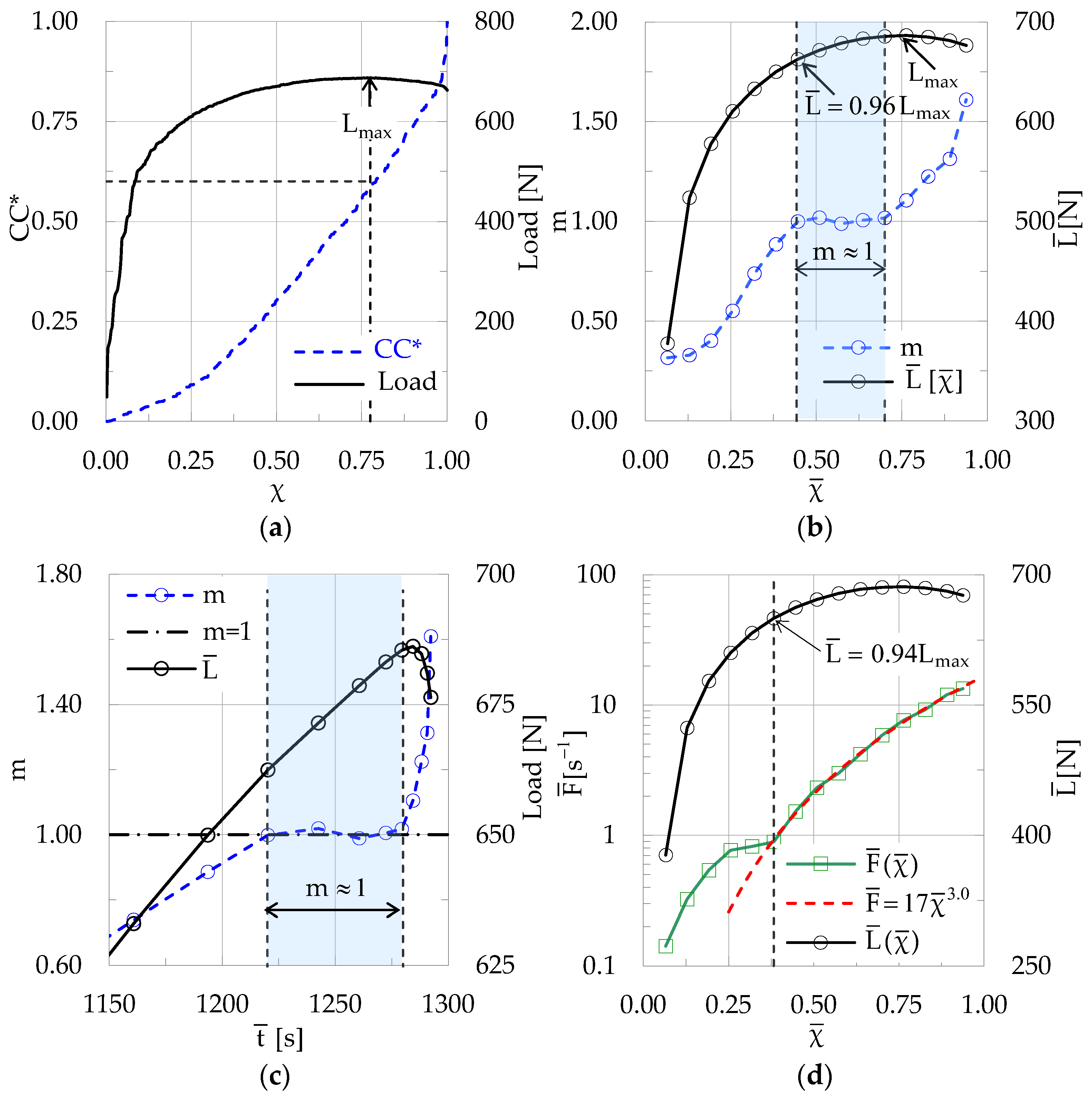
During the typical experiment (that will be discussed here) of the specific protocol N = 315 acoustic hits were recorded in total, from the onset of loading up to the instant of macroscopic fracture. About 60% of them were recorded before the applied load attained its peak value, which was equal to L_max = 687 N. The evolution of the normalized Cumulative Counts, CC*, in terms of Natural Time, χ, is plotted in Figure 14a, in juxtaposition to the respective evolution of the applied load.

Using the “sliding window” procedure with sub-groups of n = 40 successive hits and a “sliding step” of Δn = n/2 = 20 hits, the respective numerical values of m and $\overline{\mathrm{L}}$ were determined and paired to the average Natural Time, $\overline{\mathrm{\chi }}$. Both functions m($\overline{\mathrm{\chi }}$) and $\overline{\mathrm{L}}$($\overline{\mathrm{\chi }}$) are plotted in Figure 14b.

The evolution of m is quite compatible to that of the protocol with DEN specimens (Sub-Section 4.1), and also, to the main protocol of the present study (Section 3). Indeed, during the early loading stages m starts from relatively low values, well below unity, which increase smoothly towards the m ≈ 1 plateau, attained at the “instant” $\overline{\mathrm{\chi }}$ ≈ 0.44. At that “instant” the average applied load is equal to $\overline{\mathrm{L}}$ ≈ 662 N, or, equivalently, $\overline{\mathrm{L}}$ ≈ 0.96L_max. From this instant on, the m-values increase rapidly towards the global maximum value m_max ≈ 1.60 attained almost at the instant of macroscopic fracture.

The “duration” of the m ≈ 1 plateau covers now the interval 0.44 < $\overline{\mathrm{\chi }}$ < 0.70, or, in other words, until an average load level $\overline{\mathrm{L}}$ ≈ 685 N that is almost equal to the peak load attained. The specific Natural Time “interval” corresponds to a conventional time interval of about Δ$\overline{\mathrm{t}}$ ≈ 60 s, as it can be seen in Figure 14c, in which the evolution of m is plotted versus the average conventional time, $\overline{\mathrm{t}}$, for the last 150 s of the test’s duration. For the specific experiment the duration of the last loading stage (i.e., the stage after the m-values start increasing again after the termination of the m ≈ 1 plateau) is equal to only 10 s.

The law of Equation (9) dictates the evolution of $\overline{\mathrm{F}}$, from the Natural Time “instant” $\overline{\mathrm{\chi }}$ ≈ 0.38 (at which the load level is equal to about 94% of the respective peak value attained). It covers the range of $\overline{\mathrm{\chi }}$-values until the “instant” $\overline{\mathrm{\chi }}$ ≈ 0.95. At that instant the load is in its descending branch and the final fracture is immediately impending.

Regarding, finally, the evolution of the average rate, $\overline{\mathrm{F}}$, of generation of acoustic hits in the Natural Time Domain, the respective results (obtained by means of the “sliding window” process with the same sub-groups and the same “sliding step” used for the determination of m) are plotted in Figure 14d. It was found that the response of the specimens of the 3PB protocol are, again governed by a power law, which is now written as:

$$\overline{\mathrm{F}} = 17{ \overline{\mathrm{\chi } }}^{3.0}$$

(9)

4.3. Some Thoughts About the Physical Interpretation of the m ≈ 1 Plateau

Taking into account the definition of parameter m, it can be said that the m ≈ 1 plateau corresponds to a stage of the loading procedure at which the normalized number of cumulative counts of the acoustic signals becomes equal to the respective average value of all the hits recorded during the specific experiment. From this instant on, signals with higher energy content are generated responsible for hits with increased amplitude and increased number of counts, leading to m-values significantly exceeding the m = 1 limit and heralding a transition of the damage mechanisms activated within the bulk of the loaded element. From the perspective of Continuous Damage Mechanics, the physical interpretation of the m ≈ 1 plateau could be deeper understood as a transition between distinct regimes of microstructural degradation. During the initial stages of uniaxial compression, microcrack activity within the Dionysos marble specimens is characterized by a random, spatially dispersed nucleation process. At this stage, the acoustic emission events are significantly uncorrelated, resulting to values of m that remain well below unity. As the level of the applied stress increases, the system undergoes a critical “translation”, reflected to the stabilization of the parameter m and the formation of the characteristic m ≈ 1 plateau, which designates the entrance into a coordinated stage of “quasi-steady state” damage aggregation. From this point on, the already formatted microcracks cease behaving independently. The respective local stress fields around them start interacting with each other, leading to an accelerated yet stable coalescence. In this context the m ≈ 1 plateau reflects a self-organized critical state where the energy release and damage accumulation approach a dynamic equilibrium. The microcracks are actively converging toward the formation of macro-cracks, but the damage evolution has not yet entered the unstable, uncontrollable avalanche phase. Once this quasi-steady aggregation stage terminates, m increases rapidly, heralding the abrupt transition into the critical stage of impending macroscopic fracture. Interpreting the m ≈ 1 plateau through this mechanistic lens underscores its validity as a robust physical precursor, demonstrating the efficacy of the event-driven Natural Time Domain in capturing the intrinsic laws of material failure.

It is to be mentioned at this point that the key issue for the application of the method discussed here is the fact that the advantages offered by analyzing the experimental data in the Natural Time Domain were exploited. To make this statement clearer it is suggested to reconsider the physical content of parameter m. According to its definition, m quantifies the average rate of change of the normalized Cumulative Counts of the acoustic hits with respect to average Natural Time $\overline{\mathrm{\chi }}$. Taking into consideration that $\overline{\mathrm{\chi }}$ is intrinsically an event-based evolution coordinate (recall that χ_k = k/N), the analysis described in this study reflects inherently the sequential accumulation of internal micro-cracking. On the other hand, in the conventional time domain any change of the externally imposed loading rate alters, in turn, the temporal evolution of the acoustic signals recorded, rendering the identification of pre-failure indices highly dependent on the specific loading conditions imposed externally. On the contrary, the present analysis revealed that in the Natural Time Domain, this dependence on external kinematic parameters is rather effectively isolated from the dynamics of damage evolution itself. Indeed, while the specific “instants” of onset and, termination, and the total duration of the m ≈ 1 plateau are linear functions of the loading rate, the overall evolution of the m = m($\overline{\mathrm{\chi }}$) function is not affected, being stabilized systematically around the m = 1 limit for all experiments without any exception. This linear dependence suggests that the onset of the plateau could serve as a reliable pre-failure index for Structural Health Monitoring purposes. Furthermore, the superiority of the analysis in the Natural Time Domain is highlighted by its capacity to unveil the transition from reversibility to irreversibility, also in terms of the average rate of generation of acoustic hits. The evolution of this parameter is governed by a specific power law, the onset of which corresponds to the transition of the material to its non-linear response (which for brittle rock-like materials is almost identical to the transition to irreversible damage) and is in good agreement with the “instant” of onset of the m ≈ 1 plateau.

5. Conclusions

The evolution of the average rate m of change of the Cumulative Counts was studied in the Natural Time Domain, taking advantage of experimental data regarding the Acoustic Emissions recorded in a protocol with Dionysos marble specimens submitted to uniaxial compression under load-controlled conditions with various loading rates. The present study is part of a wider ongoing project aiming to the detection (and assessment of effectiveness) of signals that can be used as pre-failure indices for practical Structural Health Monitoring purposes. The conclusions drawn can be summarized as follows:

In all experiments, without any exception, the evolution of m in the Natural Time Domain is characterized by a specific motif: Starting from relatively low values (in any case well below unity) m increases systematically towards a limiting value equal to m ≈ 1. After attaining this limiting value, a plateau is formed during which the values of m are maintained almost constant equal to 1. The starting “instant” of this plateau depends strongly on the loading rate. At least for the interval of loading rates used in the present study this dependence appears to be perfectly linear. The same is true for the terminal point of the plateau. Given that the slopes of these two relationships are significantly different from each other, the “duration” (extent) of the plateau increases with increasing loading rate.

After the termination of the m ≈ 1 plateau, the rate of change of m increases rapidly designating generation of acoustic events with increased number of counts and, therefore, increased energy content, heralding entrance to the critical stage of impending fracture. Comparing the quantitative data concerning the appearance and duration of the above plateau, with the data concerning the average rate of generation of acoustic signals it is suggested that the onset of the m ≈ 1 plateau could be a potentially interesting (and flexible) pre-failure indicator. Moreover, the specific index may be characterized as “objective”, since the counts of the acoustic hits is a parameter more or less independent from subjective decisions concerning the parametrization of the experimental set-up used to detect and record the AEs.

It was also concluded that the evolution of the average rate of generation of acoustic hits in the Natural Time Domain is governed by a specific power law. The onset of validity of this law is very close to the instant of transition of the response of the loaded specimen from its linear (reversible) to its non-linear (irreversible) stage of response.

The conclusions drawn from the analysis of the acoustic data of the present protocol (with Dionysos marble specimens under uniaxial compression) were juxtaposed to the respective findings from (previously published) experimental protocols with direct tension of DEN specimens and 3PB of notched beams, both made of Dionysos marble. The qualitative similarity of the results is quite satisfactory, suggesting a kind of universality of the conclusions drawn about the potentialities of the appearance of the m ≈ 1 plateau to be inherently related to entrance of loaded marble specimens into the stage of impending fracture, independently of the loading scheme adopted. It is believed, however, that it is still very early to draw definite conclusions. Additional protocols with broader variety of materials and loading schemes must be analyzed. Along these lines, the authors’ team studies the potentialities of additional thresholds uncovered while analyzing the evolution of the energy and the entropy of the acoustic signals. It can be said that the preliminary results are quite encouraging. However, and in spite of these encouraging results, it is suggested that at the present stage of progress of these efforts, the method for detecting pre-failure warning indices based on the rate of change of the normalized number of Cumulative Counts (CC*), m, in the Natural Time Domain to be considered as complementary to already existing approaches rather than as a self-standing one.

References

1. Grosse, C.U. Introduction. In Acoustic Emission Testing; Grosse, C.U., Ohtsu, M., Aggelis, D.G., Shiotani, T., Eds.; Springer Tracts in Civil Engineering; Springer: Cham, Switzerland, 2022. [Google Scholar]
2. Jia, X.; Li, J.; Zhang, Q.; Zhang, M.; Jin, Y.; Ding, Y. Analysis of critical states based on acoustic emission signals during progressive failure of wood. PLoS ONE 2024, 19, e0302528. [Google Scholar] [CrossRef] [Scilit] [PubMed]
3. Xu, Y.; Borrego, A.G.; Planes, A.; Ding, X.; Vives, E. Criticality in failure under compression: Acoustic emission study of coal and charcoal with different microstructures. Phys. Rev. E 2019, 99, 33001. [Google Scholar] [CrossRef] [Scilit]
4. Vallianatos, F.; Benson, P.; Meredith, P.; Sammonds, P. Experimental evidence of a non-extensive statistical physics behaviour of fracture in triaxially deformed Etna basalt using acoustic emissions. EPL (Europhys. Lett.) 2012, 97, 58002. [Google Scholar] [CrossRef] [Scilit]
5. Zheng, Y.; Liu, C.; Lu, K.; Zhang, H.; Jian, B.; Zhang, W. Study on the fracture behavior and critical slowing down characteristics of saturated sandstone based on acoustic emission and resistivity. Sci. Rep. 2025, 15, 12113. [Google Scholar] [CrossRef] [Scilit] [PubMed]
6. Wei, Y.; Li, Z.; Kong, X.; Zhang, Z.; Cheng, F.; Zheng, X.; Wang, C. The precursory information of acoustic emission during sandstone loading based on critical slowing down theory. J. Geophys. Eng. 2018, 15, 2150–2158. [Google Scholar] [CrossRef] [Scilit]
7. Triantis, D.; Pasiou, E.D.; Stavrakas, I.; Kourkoulis, S.K. Revealing the proximity of concrete specimens to their critical damage level by exploring the cumulative counts of the Acoustic Emissions in the Natural Time Domain. Materials 2024, 17, 1017. [Google Scholar] [CrossRef] [Scilit] [PubMed]
8. Colombo, S.; Main, I.G.; Forde, M.C. Assessing damage of reinforced concrete beam using “b-value” analysis of acoustic emission signals. J. Mater. Civ. Eng. 2003, 15, 280–286. [Google Scholar] [CrossRef] [Scilit]
9. Rao, M.V.M.S.; Lakshmi, K.P. Analysis of b-value and improved b-value of acoustic emissions and accompanying rock fracture. Curr. Sci. 2025, 89, 1577–1582. [Google Scholar]
10. Triantis, D.; Stavrakas, I.; Loukidis, A.; Pasiou, E.D.; Kourkoulis, S.K. A Study on the Fracture of Cementitious Materials in Terms of the Rate of Acoustic Emissions in the Natural Time, Domain. Appl. Sci. 2023, 13, 6261. [Google Scholar] [CrossRef] [Scilit]
11. Matsuyama, K.; Katsuragi, H. Power law statistics of force and acoustic emission from a slowly penetrated granular bed. Nonlinear Process. Geophys. 2014, 21, 1–8. [Google Scholar] [CrossRef] [Scilit]
12. Azim, A.A.; Beke, D.L.; Tóth, L.Z.; Daróczi, L. Transfer distortions of acoustic emission signals—Power relations between the signal parameters and normalized temporal shapes of avalanches. Sci. Rep. 2025, 15, 39107. [Google Scholar] [CrossRef] [Scilit] [PubMed]
13. Wang, X.; Wang, E.; Liu, X. Damage characterization of concrete under multi-step loading by integrated ultrasonic and acoustic emission techniques. Constr. Build. Mater. 2019, 221, 678–690. [Google Scholar] [CrossRef] [Scilit]
14. Niccolini, G.; Lacidogna, G.; Carpinteri, A. Fracture precursors in a working girder crane: AE natural-time and b-value time series analyses. Eng. Fract. Mech. 2019, 210, 393–399. [Google Scholar] [CrossRef] [Scilit]
15. Loukidis, A.; Pasiou, E.D.; Sarlis, N.V.; Triantis, D. Fracture analysis of typical construction materials in natural time. Phys. A 2020, 547, 123831. [Google Scholar] [CrossRef] [Scilit]
16. Friedrich, L.F.; Cezar, E.S.; Colpo, A.B.; Tanzi, B.N.; Lacidogna, G.; Ignacio Iturrioz, I. Identifying impending failure in heterogeneous materials: A study on acoustic emission time series. Chaos Solitons Fractals 2024, 185, 115172. [Google Scholar] [CrossRef] [Scilit]
17. Vidya Sagar, R.; Raghu Prasad, B.K. AE energy release during the fracture of HSC beams. Mag. Concr. Res. 2009, 61, 419–435. [Google Scholar] [CrossRef] [Scilit]
18. Sagasta, F.; Zitto, M.E.; Piotrkowski, R.; Benavent-Climent, A.; Suarez, E.; Gallego, A. Acoustic emission energy b-value for local damage evaluation in reinforced concrete structures subjected to seismic loadings. Mech. Syst. Signal Process 2018, 102, 262–277. [Google Scholar] [CrossRef] [Scilit]
19. Wu, K.; Chen, B.; Yao, W. Study of the influence of aggregate size distribution on mechanical properties of concrete by acoustic emission technique. Cem. Concr. Res. 2001, 31, 919–923. [Google Scholar] [CrossRef] [Scilit]
20. Varotsos, P.; Sarlis, N.V.; Skordas, E.S. Natural Time Analysis: The New View of Time. Precursory Seismic Electric Signals, Earthquakes and Other Complex Time-Series; Springer Science and Business Media: Berlin/Heidelberg, Germany, 2011. [Google Scholar]
21. Kourkoulis, S.K.; Pasiou, E.D.; Loukidis, A.; Stavrakas, I.; Triantis, D. Comparative assessment of criticality indices extracted from acoustic and electrical signals detected in marble specimens. Infrastructures 2022, 7, 15. [Google Scholar] [CrossRef] [Scilit]
22. Vallianatos, F.; Michas, G.; Benson, P.; Sammonds, P. Natural time analysis of critical phenomena: The case of acoustic emissions in triaxially deformed Etna basalt. Phys. A 2013, 392, 5172–5178. [Google Scholar] [CrossRef] [Scilit]
23. Niccolini, G.; Potirakis, S.M.; Lacidogna, G.; Borla, O. Criticality hidden in acoustic emissions and in changing electrical resistance during fracture of rocks and cement-based materials. Materials 2020, 13, 5608. [Google Scholar] [CrossRef] [Scilit] [PubMed]
24. Zhu, Z.; Jiang, Z.; Accornero, F. Size-scale and time-scale effects on the failure of UHPC-strengthened reinforced concrete beams. Structures 2025, 78, 109248. [Google Scholar]
25. Naukhez, K.; Vidya Sagar, R.; Chandra Kishen, J.M. Q-Statistical analysis of Acoustic Emissions recorded during unconfined uniaxial compression of ultra-high-performance concrete. In Proceedings of the 11th International Conference on Fracture Mechanics of Concrete and Concrete Structures, Bangalore, India, 10–14 September 2023. [Google Scholar]
26. Niccolini, G.; Manuello, A.; Marchis, E.; Carpinteri, A. Signal frequency distribution and natural-time analyses from acoustic emission monitoring of an arched structure in the Castle of Racconigi. Nat. Hazards Earth Syst. Sci. 2017, 17, 1025–1032. [Google Scholar] [CrossRef] [Scilit]
27. Lacidogna, G.; Friedrich, L.F.; Marin Montanari, P.; Hamdan Padilha, M.; Invernizzi, S.; Di Tommaso, A.; Iturrioz, I. A multi-technique approach to long-term structural health monitoring of the Garisenda Tower (Italy). Struct. Health Monit. 2026, 14759217261448084. [Google Scholar]
28. Triantis, D.; Kourkoulis, S.K. An alternative approach for representing the data provided by the acoustic emission technique. Rock Mech. Rock Eng. 2018, 51, 2433–2438. [Google Scholar] [CrossRef] [Scilit]
29. Zambas, C. Mechanical Properties of Pentelik Marbles; Committee for the Restoration of Parthenon Publications: Athens, Greece, 1994. [Google Scholar]
30. Theocaris, P.S.; Coroneos, E. Experimental study of the stability of Parthenon. Publ. Acad. Athens 1979, 44, 1–80. [Google Scholar]
31. Kaklis, K.; Maurigiannakis, S.; Agioutantis, Z.; Istantso, C. Influence of Specimen Shape on the indirect tensile strength of transversely isotropic dionysos marble using the three-point bending test. Strain 2009, 45, 393–399. [Google Scholar] [CrossRef] [Scilit]
32. Cardani, G.; Meda, A. Flexural strength and notch sensitivity in natural building stones: Carrara and Dionysos marble. Constr. Build. Mater. 1999, 13, 393–403. [Google Scholar] [CrossRef] [Scilit]
33. Kourkoulis, S.K.; Exadaktylos, G.E.; Vardoulakis, I. U-notched Dionysos-Pentelicon marble in three point bending: The effect of nonlinearity, anisotropy and microstructure. Int. J. Fract. 1999, 98, 369–392. [Google Scholar] [CrossRef] [Scilit]
34. Papadopoulos, C.; Basanou, M.E.; Vardoulakis, I. Mechanical behaviour of Dionysos marble smooth joints: I. Experiments. In Mechanics of Jointed and Faulted Rock; Rossmanith, H.P., Ed.; Routledge: Oxfordshire, UK, 1998. [Google Scholar]
35. Landis, E.N.; Baillon, L. Experiments to relate acoustic emission energy to fracture energy of concrete. J. Eng. Mech. 2002, 128, 698–702. [Google Scholar] [CrossRef] [Scilit]
36. Niu, Y.; Zhou, X.P. Forecast of time-of-instability in rocks under complex stress conditions using spatial precursory AE response rate. Int. J. Rock Mech. Min. Sci. 2021, 147, 104908. [Google Scholar] [CrossRef] [Scilit]
37. Loukidis, A.; Triantis, D.; Stavrakas, I.; Pasiou, E.D.; Kourkoulis, S.K. Detecting criticality by exploring the acoustic activity in terms of the “Natural-Time” concept. Appl. Sci. 2022, 12, 231. [Google Scholar]
Figure 1. The evolution of the function of the normalized Cumulative Counts CC*(χ) versus Natural Time, χ, in juxtaposition to the respective evolution of the externally applied normalized stress, σn.
Applsci 16 06399 g001
Figure 2. (a) The axial stress-axial strain plot for a typical experiment of the preliminary protocol; (b) a typical instrumented specimen of the main protocol before being loaded.
Applsci 16 06399 g002
Figure 3. The evolution of the normalized Cumulative Counts (CC*) versus (a) the conventional time, t, and (b) the Natural Time χ, juxtaposed to the respective evolution of the applied axial stress.
Applsci 16 06399 g003
Figure 4. The evolution of the rate of change of the normalized number of Cumulative Counts (CC*), m, in the Natural Time Domain (i.e., the evolution of the slope of the m = m( χ ¯ ) function) juxtaposed to that of the average stress, σ ¯ n .
Applsci 16 06399 g004
Figure 5. A fictitious function CC ¯ * (χ) for an experiment with all its hits having the same number of counts (dashed straight line), equal to the mean value of the counts of the hits of the experiment of Figure 3. The actual CC*(χ) function is plotted, also (continuous blue line).
Applsci 16 06399 g005
Figure 6. The evolution of the rate m of change of the normalized Cumulative Counts (CC*) in the Natural Time Domain, in juxtaposition to the respective evolution of the normalized average stress applied, for loading rates equal to (a) 95 kPa/s; (b) 145 kPa/s; (c) 350 kPa/s.
Applsci 16 06399 g006
Figure 7. (a) The dependence of the starting and the terminal “instants”, σ ¯ n , s and σ ¯ n , e , respectively, of the m ≈ 1 plateau, as well as that of its “duration” Δ σ ¯ n m 1 , on the loading rate; (b) the dependence of the duration of the m ≈ 1 plateau (in terms of the conventional time t) on the loading rate.
Applsci 16 06399 g007
Figure 8. The evolution of the average rate F ¯ of generation of acoustic hits versus (a) the average conventional time, t ¯ , and (b) the average Natural Time, χ ¯ . In both figures, the respective evolution of the normalized average stress applied, σ ¯ n , is also plotted.
Applsci 16 06399 g008
Figure 9. The evolution of the average rate F ¯ of generation of acoustic hits versus the average Natural Time, χ ¯ , for the specimens loaded at rates equal to (a) 95 kPa/s, (b) 145 kPa/s, and (c) 350 kPa/s.
Applsci 16 06399 g009
Figure 10. The dependence of the σ ¯ n ( χ ¯ p ) threshold (designating the onset of the validity of the power law of Equation (7)) on the loading rate imposed, in juxtaposition to the respective dependence of the σ ¯ n , s threshold (designating the onset of the m ≈ 1 plateau, as it was discussed in Section 3.2).
Applsci 16 06399 g010
Figure 11. Geometry and dimensions of the specimens of the (a) DEN- and (b) 3PB- protocols.
Applsci 16 06399 g011
Figure 12. The evolution of the normalized Cumulative Counts CC* in terms of the (a) Natural Time, χ, and (b) the conventional time, t. Only the very last loading stage is shown in (b).
Applsci 16 06399 g012
Figure 13. The evolution of m in terms of (a) the average Natural Time, χ ¯ , and (b) the average conventional time, t ¯ ; (c) the evolution of the average rate F ¯ of generation of acoustic hits in the Natural Time Domain. The respective evolution of the load applied is, also, juxtaposed in all three figures.
Applsci 16 06399 g013
Figure 14. (a) The evolution of the normalized Cumulative Counts CC* in terms of the Natural Time, χ; the evolution of m (b) in terms of the average Natural Time, χ ¯ , and (c) in terms of the average conventional time, t ¯ ; (d) the evolution of the average rate F ¯ of generation of acoustic hits in the Natural Time Domain. The respective evolution of the load applied is, also, juxtaposed in all figures.
Applsci 16 06399 g014