A Discrete-Time Suboptimal Robust MPC Framework for Systems with Inverse-Proportional Dynamics

Abstract

This study presents the development and implementation of a robust model predictive control (MPC) strategy for dynamically inverse-proportional systems. Such systems arise frequently in practical settings, particularly in applications involving electronic sensors, among other domains. However, the existing literature lacks a comprehensive and systematic design framework for robust MPC specifically tailored to this class of systems. To address this gap, we realize an inverse-proportional system by employing a Van der Pol oscillator in conjunction with a low-pass filter stage. For the purpose of robust MPC design, a dynamically inverse-proportional system is modeled as a linear perturbed system characterized by a negative gain in the input channel. This formulation is considered within the discrete-time control framework, where a suboptimal control problem is effectively formulated. Furthermore, the explicit realization of an inverse-proportional system enables a rigorous assessment of controller performance in this setting. The effectiveness of the proposed control scheme is supported through a reproducible numerical experiment, which serves as validation of the approach.

1. Introduction

A dynamic system that responds inversely to its control input is one where an increase in the input causes a decrease in the output [1,2]. For example, the force of gravity between two masses is inversely proportional to the square distance between their centers. In the financial environment, risk and return shares have an inverse relationship. Some electronic sensors react inversely to a physical parameter [3,4]. Moreover, inverse design is a methodology that reverses the conventional design process, proceeding from desired outputs to the prediction of input parameters. For example, although data-driven inverse design has achieved notable success in fields such as mechanics, photonic, and materials science (see [5,6,7], and references therein), it still lacks successful applications in the domain of flexible sensors [8]. Therefore, the control of inverse systems remains an area requiring further investigation.

Controlling a dynamic system that responds inversely to its control input is considered an important challenge. Among the available control methodologies, we selected the Robust Model Predictive Control (RMPC) algorithm due to its reduced computational complexity when applied to linear systems [9]. Although Van der Pol systems are a nonlinear third order system, a linearized inverse proportional dynamical system is considered, including the low-pass filter. Although RMPC was traditionally used for slow dynamical systems, it is now feasible to apply it to fast dynamical systems as well [10]. Moreover, RMPC is a control technique widely adopted in some industrial processes [11,12,13,14]. Furthermore, RMPC can handle the system’s constraints and nonlinearities [15]. Additionally, RMPC can be used along with other techniques to increase its performance [16,17]. RMPC is a discrete-time control methodology where, at each instant of time, this technique requires the online solution of an optimization scheme subject to constraints in an infinite time horizon [9]. Although more than one control move is obtained, only the first one is realized. This process is then repeated at each sampling time [9]. Generally, Linear Matrix Inequality (LMI) theory is used in the constrained optimization problem. For a real application of a robust model predictive control with an integral action, see [18]. This reference may be suitable for teaching courses on control engineering. Furthermore, robust model predictive control can be invoked to minimize operating costs [19].

Voltage-controlled oscillators (VCOs) are widely used in communication systems [20]. In addition, various sensor platforms, including micro-electromechanical systems, motion detection units, impedance spectroscopy setups, and others, employ VCOs as a core element [21]. From a mathematical standpoint, a voltage-controlled oscillator can be modeled using the Van der Pol equation [22]. Notably, the Van der Pol system is versatile enough to be tuned specifically for use as a harmonic oscillator [23]. The Van der Pol oscillator is a non-conservative yet stable system known as a relaxation oscillator. Since its discovery, it has been widely used to study the behavior of nonlinear oscillators and various oscillatory phenomena in both physical and biological systems. Applications include the analysis of electrical circuits [24], modeling of the heartbeat [25], and the study of neuronal action potentials [26]. Therefore, we developed an inverse proportional dynamical system for numerical experiments by invoking a modified Van der Pol (VDP) system and low-pass filtering stage. Hence, the main objective of this paper is to highlight the performance of a robust model predictive control technique to an inverse proportional dynamical system. Furthermore, when designing the RMPC, an inverse proportional system can be viewed as a linear perturbed system with a negative gain on the canal input signal. This is because the RMPC is a statement on the discrete-time domain. The main contributions of this paper are summarized as the design of an RMPC strategy for a VDP system (which is a nonlinear third-order system) incorporating a low-pass filter. To achieve this, a novel inverse-proportional dynamic model is proposed. This new system is a linear one, reproducing the VDP system plus the filter, and then linear RMPC can be used, improving the computational complexity. A condition on the discrete sampling rate is also derived as a function of a single system parameter, resulting in a simple implementation algorithm. Notice that numerical simulations are conducted utilizing the original nonlinear system, with execution carried out through the Python programming language.

Motivation. In recent years, the theory of MPC has grown exponentially. For instance, in [14], the authors present the Tube-Based RMPC, an online optimization-based method which can handle constraints and uncertainties as well. The main problem of this approach is that this method is based on considering the worst-case scenario of the uncertainties. They propose a learning-based Gaussian process regression to overcome this problem, but then, the computational complexity is increased. In [27], a deep learning-based model predictive control algorithm is used to approximate the uncertainties. In [28], a Lyapunov-based nonlinear MPC is designed to compensate disturbances, using neural networks to ensure the system’s convergence. For an overview of RMPC, see [29], where some robust methods are presented. The main objective of our proposal is to obtain a simple-to-implement RMPC; so, our approach is better in this sense, ensuring the main goal of robust MPC, that is, to devise an optimization-based control synthesis method that accounts for the intricate interactions of the uncertainty with the system, constraints, and performance criteria in a computationally tractable way. Specifically, a closed-form suboptimal MPC controller is considered, with Lyapunov theory employed to prove its robustness. Moreover, RMPC’s ability to predict system behavior and enforce constraints while optimizing a performance objective is therefore a central motivation for its use in industry.

2. Inverse Proportional System Modeling

This section focuses on our inverse proportional system model derived from the Van der Pol system, which is then followed by a low-pass filter. To start, we present the Van der Pol system [23]:

$$\ddot{x}\left(t\right)+ϵ\left[{(x\left(t\right)-x_0)}^2-{\rho }^2\right]\dot{x}\left(t\right)+{\mu }^2(x\left(t\right)-x_0)=0,$$

(1)

where $x\left(t\right)$ and $\dot{x}\left(t\right)$ represent the oscillating signals; $\rho$ governs the amplitude of oscillation, $\mu$ determines the frequency, $ϵ$ influences the transient response, and $x_0$ indicates the average value. The parameters $\rho ,ϵ$, and $\mu$ are all positive constants. The initial conditions are not necessarily zero. Additionally, the system represented in Equation (1) can be expressed as follows:

$$\begin{array}{ccc}\hfill {\dot{x}}_1\left(t\right)& =& x_2\left(t\right)\hfill \\ \hfill {\dot{x}}_2\left(t\right)& =& -ϵ\left[{(x_1\left(t\right)-x_0)}^2-{\rho }^2\right]x_2\left(t\right)-u\left(t\right)\left[x_1\left(t\right)-x_0\right],\hfill \end{array}$$

(2)

where $u\left(t\right)={\mu }^2\left(t\right)$ now serves as our control input command. In order to expand the control domain, we will examine a broader scenario in which $u\left(t\right)=f\left(t\right)$. We will also consider that this variable may assume negative values. It is widely recognized that the Van der Pol (VDP) system demonstrates an asymptotically stable limit cycle [23]. For our analysis, we will employ the parameter values $\rho =1$, $ϵ=0.1$, and $x_0=0$. These parameters are akin to those typically seen in academic examples of the Van der Pol system, although they can certainly be modified to suit specific experimental situations. The response of the VDP system described in Equation (2) is illustrated in Figure 1.

To complete our inverse proportional system, we configure the system shown in Figure 2. The transfer function of the low-pass filter is given by

$$H\left(s\right)={\displaystyle \frac{w_0}{s+w_0}},$$

(3)

where $w_0$ is the cutoff-frequency. The system described by (3) admits the alternative form:

$$\dot{y}\left(t\right)=w_0(-y\left(t\right)+z\left(t\right)),$$

(4)

where $y\left(t\right)$ is the low-pass filter output, and $z\left(t\right)$ is the internal low-pass filter variable depending on the input $x_1\left(t\right)$. The block diagram of the inverse system is illustrated in Figure 2. As shown, the input $u\left(t\right)$ is supplied to the Van der Pol oscillator to generate the output $x_1\left(t\right)$, which is subsequently filtered to yield the final system output $y\left(t\right)$. In (4), their relation is proposed as

$$z\left(t\right)=0.5x_1\left(t\right)\mathrm{sgn}\left(x_1\left(t\right)-y\left(t\right)\right).$$

(5)

The variable $z\left(t\right)$ is introduced to keep a kind of correlation between $x_1\left(t\right)$ and $y\left(t\right)$ whose chattering behavior is then filtered. The signum function $\mathrm{sgn}\left(x\right)$ is defined as 1 if $x>0$, $-1$ if $x<0$, and 0 otherwise. A low-pass filter model incorporating an internal sign function is typically used to create a nonlinear, robust, or adaptive filter that can rapidly track input changes while suppressing noise, often implemented in sliding mode control or specialized signal processing systems [30].

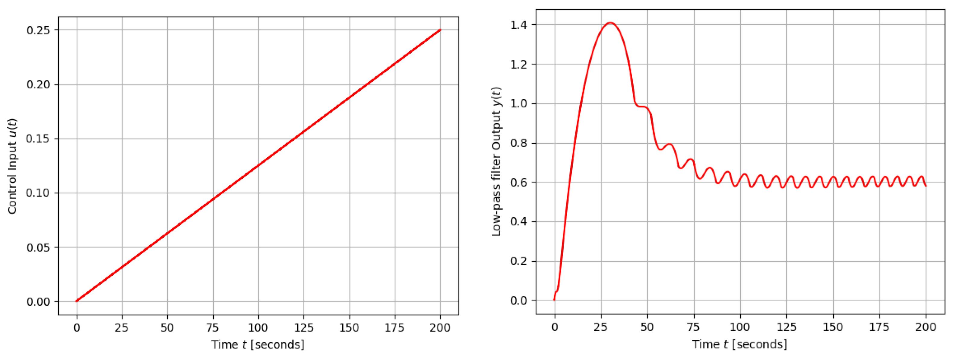
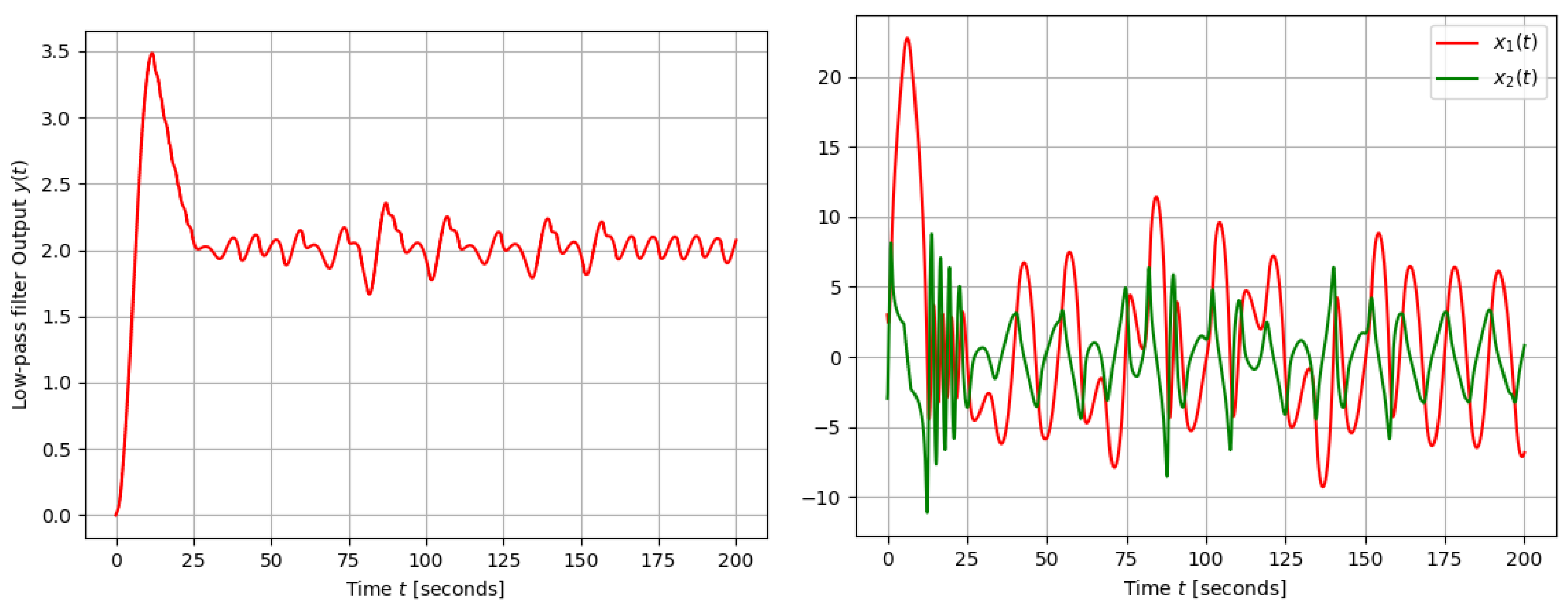
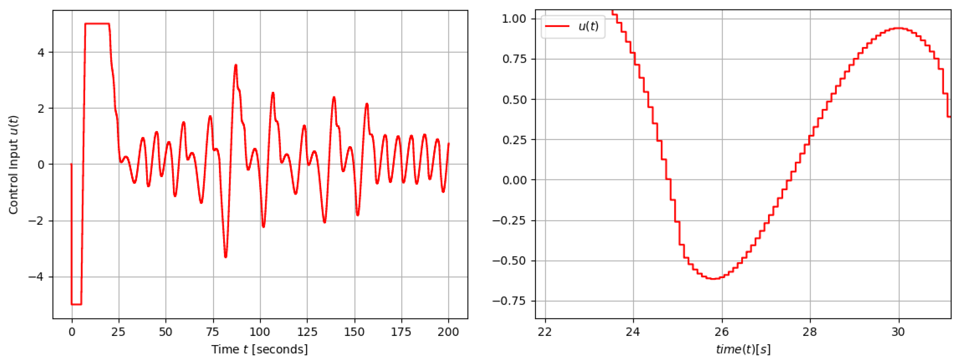
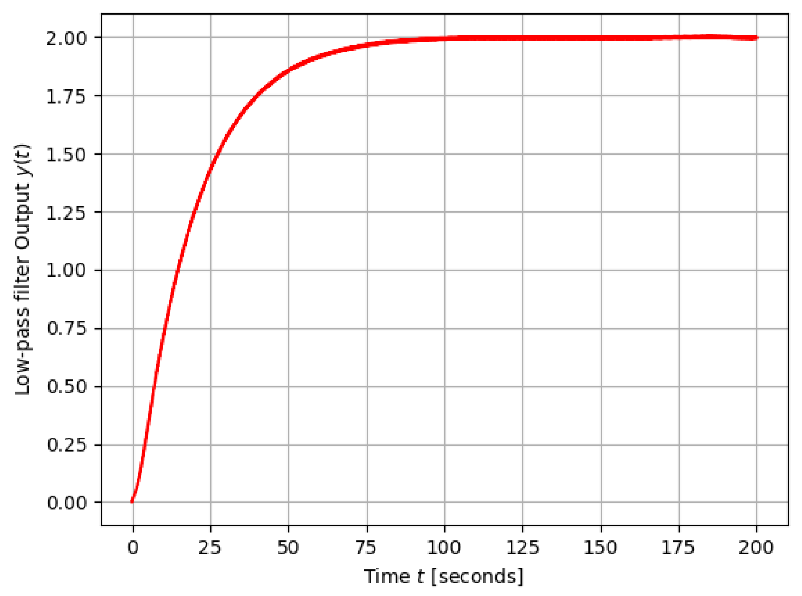
Additionally, Figure 3 shows the system’s response to our dynamic model representing an inverse proportional system with $w_0=0.05$. Hereafter, we will use this value. It is observed that the system has an oscillating component. We may consider it to have an additive perturbation for the robustness performance evaluation of our RMPC algorithm. Figure 4 shows the system’s response for the control signal $u\left(t\right)$.

3. Predictive Control Design

To facilitate the control design, we employ a specific representation of an inverse-proportional dynamical system as follows:

$$\dot{y}\left(t\right)=-ay\left(t\right)+b(u_{\max }-u\left(t\right)),$$

(6)

where a, b, and $u_{\max }$ are positive constants characterizing the system, and $u\left(t\right)$ denotes the control signal. This model is intended strictly for design objectives; consequently, precise knowledge of the parameter values is not required. However, to maintain the inherent inverse-proportional characteristics of the system, the parameters in (6) must be strictly positive. It is not mandatory to satisfy the condition $u\left(t\right)\le u_{\max }$, as the above system is a stable dynamic system. RMPC is a discrete-time framework for control design. Hence, by using the explicit Euler’s method with step time h, the discrete-time model to the system (6) yields

$$y(k+1)=Ay\left(k\right)-Bu\left(k\right)+d,$$

(7)

where $A=(1-ah)$, $B=bh$, and $d=bh{u}_{\max }+w\left(k\right)$. The uncertainty model is incorporated into the predictive formulation through the bounded disturbance $w_k$, with $ma{x}_k\left\{\right|w_k\left|\right\}\le w_{max}$. Notice that Equation (7) presents a first-order system. Hence, designing our RMPC for the system represented in Figure 2 implies the use of a first-order model to control a nonlinear third-order system described in Equations (2), (4), and (5). The RMPC design focuses on determining a state-feedback control law for the system (7) [10]:

$$u(k+i|k)=F(k\left)y\right(k+i\left|k\right),i\in N,$$

(8)

such that the following performance index be fulfilled [10]:

$$\begin{array}{c}\hfill \underset{u(k+i|k)}{\min }\max J\left(k\right)={\displaystyle \sum _{i=0}^{\infty }}q{y}^2(k+i|k)+r{u}^2(k+i|k),\end{array}$$

(9)

where $q>0$ and $r>0$ are weighting scalar values. In the RMPC technique, the plant output is measured at each sampling time k to predict its future response. Hence, $u(k+i|k)$ is the control move at time $k+i$ predicted at time k, and $u\left(k\right)=u\left(k\right|k)$ will be the action at discrete-time k [10]. This iterative process is repeated at every discrete-time sampling interval k. Here, $y(k+i|k)$ denotes the predicted system output at time $k+i$ for $i\in \mathbb{N}$. We assume that both the predicted outputs and control inputs remain within the compact sets $\overline{Y}$ and $\overline{U}$, respectively, which are subsets of $\mathbb{R}$ containing the origin as an interior point. To address the minimax optimization problem presented in (9), we define a candidate Lyapunov function $V\left(y\right(k\left|k\right))$. The goal is to determine the feedback gain $F\left(k\right)$ from (8) effectively minimizing the upper bound of the objective function $J\left(k\right)$ at each time step. So, we consider the next Lyapunov function:

$$V\left(y\left(k\right|k)\right)=y^2\left(k\right|k)$$

(10)

In order to define the RMPC function $F\left(k\right)$ (8), let us obtain the inequality $J\left(k\right)\le V\left(y\right(k\left|k\right))$ from predictions at instant $k+i$. From Equations (9) and (10), if

$$V\left(y(k+i+1|k)\right)-V\left(y(k+i|k)\right)\le -q{y}^2(k+i|k)-r{u}^2(k+i|k),$$

(11)

then by summing from $i=0$ to ∞, we obtain

$$\begin{array}{c}\hfill V\left(y\right(\infty \left|k\right))-V(y\left(k\right|k\left)\right)\le -J\left(k\right).\end{array}$$

(12)

To ensure stability over an infinite prediction horizon, we impose the condition $V\left(y\right(\infty \left|k\right))=0$, resulting in the upper bound property:

$$\begin{array}{c}\hfill J\left(k\right)\le V\left(y\right(k\left|k\right))\le \gamma <\infty ,\end{array}$$

(13)

obtaining $\gamma >0$ as an upper-bound of the performance index $J\left(k\right)$ in (9). Then, the control law in (8) is designed such that the upper bound $\gamma$ of $J\left(k\right)$ is minimized, rather than $J\left(k\right)$ itself, thereby addressing a suboptimal control problem [10]. Therefore, a suboptimal MPC controller is considered, which eliminates the need for online receding-horizon optimization.

From (10), system (13) can be also stated as $y^2(k/k)\le \gamma$. To design the state-feedback control law $F\left(k\right)$ in (8), we evaluate the left-hand side of inequality (11). Utilizing the definition of the Lyapunov function in (7) along with the discrete-time system dynamics (7), it follows that

$$\begin{array}{ccc}V\left(y\right(k+i+1\left|k\right))-V(y(k+i|k\left)\right)\hfill & =& y^2(k+i+1|k)-y^2(k+i|k)\hfill \\ & =& {\left(Ay(k+i|k)-Bu(k+i\left|k\right)+d\right)}^2-y^2(k+i|k).\hfill \end{array}$$

Using $u(k+i|k)=F(k\left)y\right(k+i\left|k\right)$ for the unperturbed case ($d=0$), inequality (11) becomes

$${\left(Ay(k+i|k)-BF(k\left)y\right(k+i\left|k\right)\right)}^2-y^2(k+i|k)\le -q{y}^2(k+i|k)-r{u}^2(k+i|k).$$

By aggregating the individual contributions in $y^2(k+i|k)$, we obtain the following expression:

$$y^2(k+i|k)\left[F^2\left(k\right)(r+B^2)-2ABF\left(k\right)+(A^2+q-1)\right]\le 0.$$

(14)

Inequality (14) holds for all $y(k+i|k)$ if and only if the following condition is met:

$$F^2\left(k\right)(r+B^2)-2ABF\left(k\right)+(A^2+q-1)\le 0.$$

(15)

Assuming a sampling interval h that ensures $0<A<1$, we can prescribe $q=1-A^2$. Consequently, the quadratic condition in (15) reduces to

$$F\left(k\right)\left[(r+B^2)F\left(k\right)-2AB\right]\le 0.$$

(16)

So, $F\left(k\right)\in (0,\frac{2AB}{r+B^2}]$. Consequently, the solution to the RMPC optimization problem is given by

$$u(k+i|k)=Ky(k+i|k),\mathrm{for}K\in \left(0,\frac{2AB}{r+B^2}\right].$$

(17)

Since the weighting parameter r can be any arbitrary positive value, the gain K may likewise be any positive constant. Furthermore, once the weighting parameter r is established, K value is strictly constrained to the interval $\left(0,\frac{2AB}{r+B^2}\right]$. Thus, the state-feedback control law in (17) is effectively represented as

$$u(k+i|k)=Ky(k+i\left|k\right)$$

(18)

for $K\in \left(0,\frac{2AB}{r+B^2}\right]$. In summary, these results lead to the following principal theorem.

Theorem 1.

A solution to the suboptimal RMPC to the system (7) is given by (18) for any $K\in \left(0,\frac{2AB}{r+B^2}\right]$ and a sampling rate h such that the parameter A satisfies $0<A<1$.

The implementation of this RMPC strategy is straightforward, as it does not rely on additional constraints or complex numerical solvers commonly found in traditional predictive control schemes. Moreover, the RMPC depends on only the design parameter step time h. Here, the inverse proportional behavior of system (7) is essential. Algorithm 1 presents the algorithm of the proposed RMPC, and used in the simulations.

Algorithm 1: RMPC algorithm

Define

h (Sampling time)

N (Number of steps to arrive to one h)

n (Simulation horizon)

K (Control parameter)

$w_0$ (Low-pass filter parameter)

Initialize plant state vector $(x_1\left(k\right),x_2\left(k\right))$

While $k<n$

If $ks<N$: $u\left[k\right]=u[k-1]$; ks+

else $u\left[k\right]=K(y\left[k\right]-y_{ref})$ as (19); ks = 0

Actualize

$(x_1\left[k\right],x_2\left[k\right])$ as (2)

$y\left[k\right]$ as (4)

The final design depends on a control gain K (17), which is defined in terms of the model parameters $A=(1-ah)$ and $B=bh$ from (6), as well as the design parameter r. To ensure robust stability against severe parametric variations in the oscillator, K must be tuned as a function of the integration step size h. Since $B>0$ and a is related to $w_0$, the condition $A=1-ah>0$ implies that $h<1/a$ and $1-a\gg 1$. Consequently, h can take any sufficiently small value, allowing the system dynamics to be integrated internally at a much finer resolution to maintain both numerical stability and tracking accuracy.

4. Simulation Results

To assess the effectiveness of the proposed approach, this section details the application of the RMPC law from Theorem 1 to the nonlinear system depicted in Figure 2. The simulation utilizes the complete system model described by Equations (2), (4), and (5). From the algorithm presented in Algorithm 1, we use a sampling rate $h=0.1$ s, $N=100$, $n=2·{10}^5$, and $w_0=0.05$. The control upper bound is set to $u_{max}=5$. The control gain is set $K=10$ as nominal value. The simulations are performed under Python 3.12.2. So, in order to see the robustness of our proposal, some simulations are carried out, where the non-simplified VDP system (2) is considered. Additionally, we use the general regulation control law given by

$$u(k+i|k)=K\left(y(k+i|k)-y_{ref}\left(k\right)\right),$$

(19)

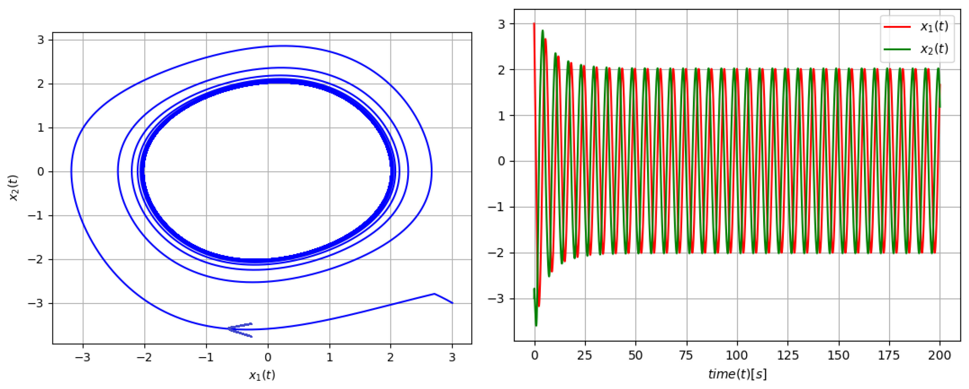
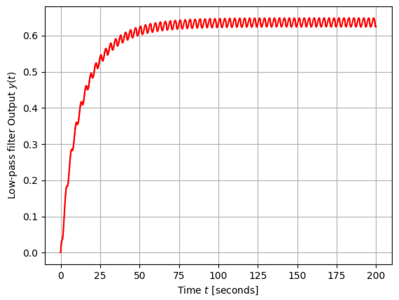
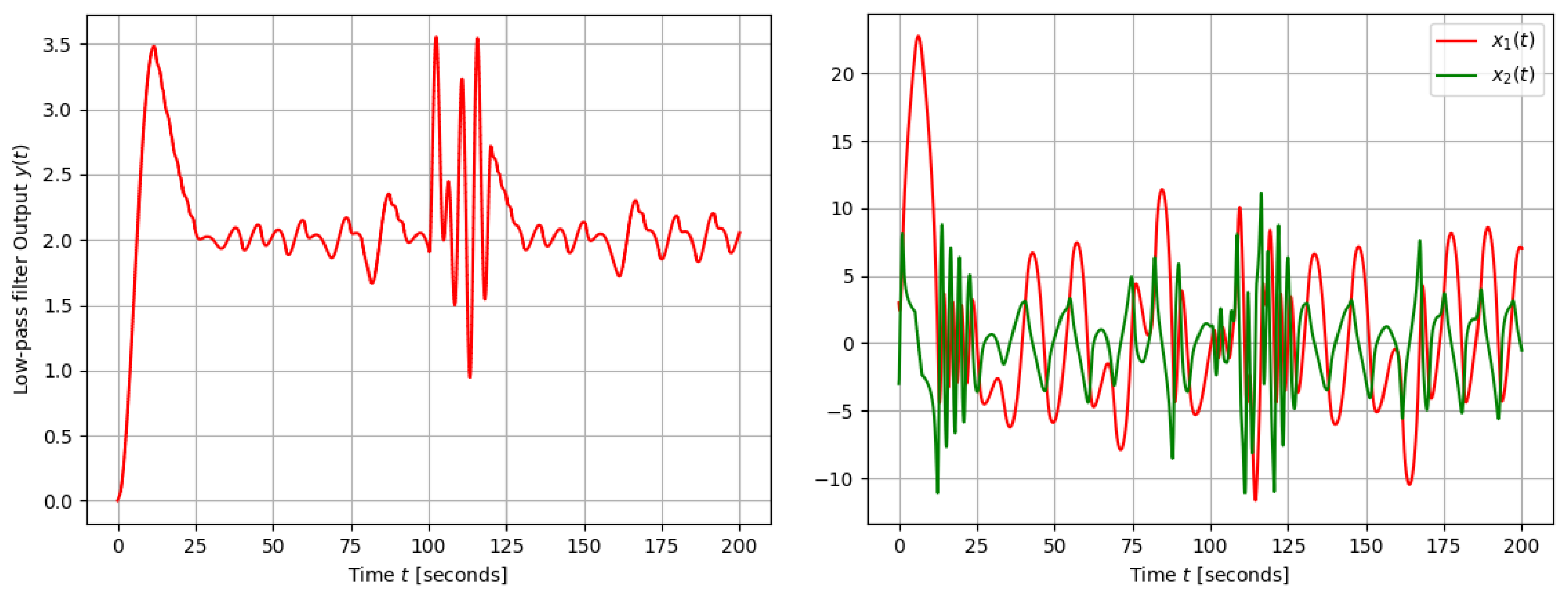
where $y_{ref}\left(k\right)=2$ represents the set-point value of the regulation control application. Figure 5, Figure 6 and Figure 7 show the performance of our RMPC control stated in (19), applied to the inverse proportional system defined by the nonlinear system VDP (2) along with the low-pass filter (4) and (5). Hence, Figure 5 (left) presents the response of VDP variables to the input RMPC (19), that is, the closed-loop system response. We can observe an oscillating behavior around the reference value. Notice that the control law was designed using the plant’s unperturbed model to control, and the Bounded-Input–Bounded-Output (BIBO) stability is confirmed.

According to [18], by considering an integral action, MPC design can enhance its performance. To do this, the control input is then $k_i\int u\left(t\right)dt$, with $k_i=-0.1$. Then, using its discrete-time representation, the obtained result is shown in Figure 7. Comparing Figure 5 (Left) and Figure 7, the system shows no oscillation, and the convergence to the reference is notable.

The closed-loop responses in Figure 5 and under integral action in Figure 7 demonstrate that the proposed RMPC effectively regulates the output while mitigating the oscillatory behavior, which is essential for reliable sensing and calibration. The approach is also relevant to voltage-controlled oscillators and oscillator-based systems, for which the Van der Pol oscillator serves as a representative model. The simulations in Figure 5 and Figure 6 show that the controller stabilizes oscillatory dynamics and ensures bounded behavior under predictive control.

5. Discussion

The main advantage of our approach is its simplicity, despite using a model-predictive controller. The robustness is already considered, as mentioned in Section 2: the oscillating term of the system can be seen as an additive perturbation. Nevertheless, an external disturbance is considered in Figure 8, where the variable $x_2\left(t\right)$ is excited by an external signal defined as sums as different sinusoidal signals, at the time interval $[100,120]$ s. The system takes approximately 15 s to follow the reference.

Here, we use RMPC, applied to inverse proportional systems to predict future behavior and calculate the optimal control input to achieve the desired response, as seen in Section 4. Among the usual control strategies, we highlight

• Adaptive Control: This method uses a deep learning network to learn the inverse of the plant’s dynamics. The learned inverse function is then used as the controller, which can be more robust and faster than traditional adaptive filtering techniques [31]. The problem is the need for persistent excitation to carry out the parametric identification, not necessary in our approach.
• PID with a Predictor: A system with inverse response will react in the opposite direction to what is intuitively expected, making it hard to control with simple methods. For example, a standard PID controller might have a poor response or struggle to stabilize the system. A common approach is to add a predictor block to a standard feedback control system to compensate for the inverse response [32]. The main problem in this approach is the definition of the predictor, creating design complexities not needed in our proposal.
• Data-Based Control: For discrete-time systems, a data-based method can be used to design a predictive controller without a prior model of the process [5]. This approach is relatively much more complex than ours.

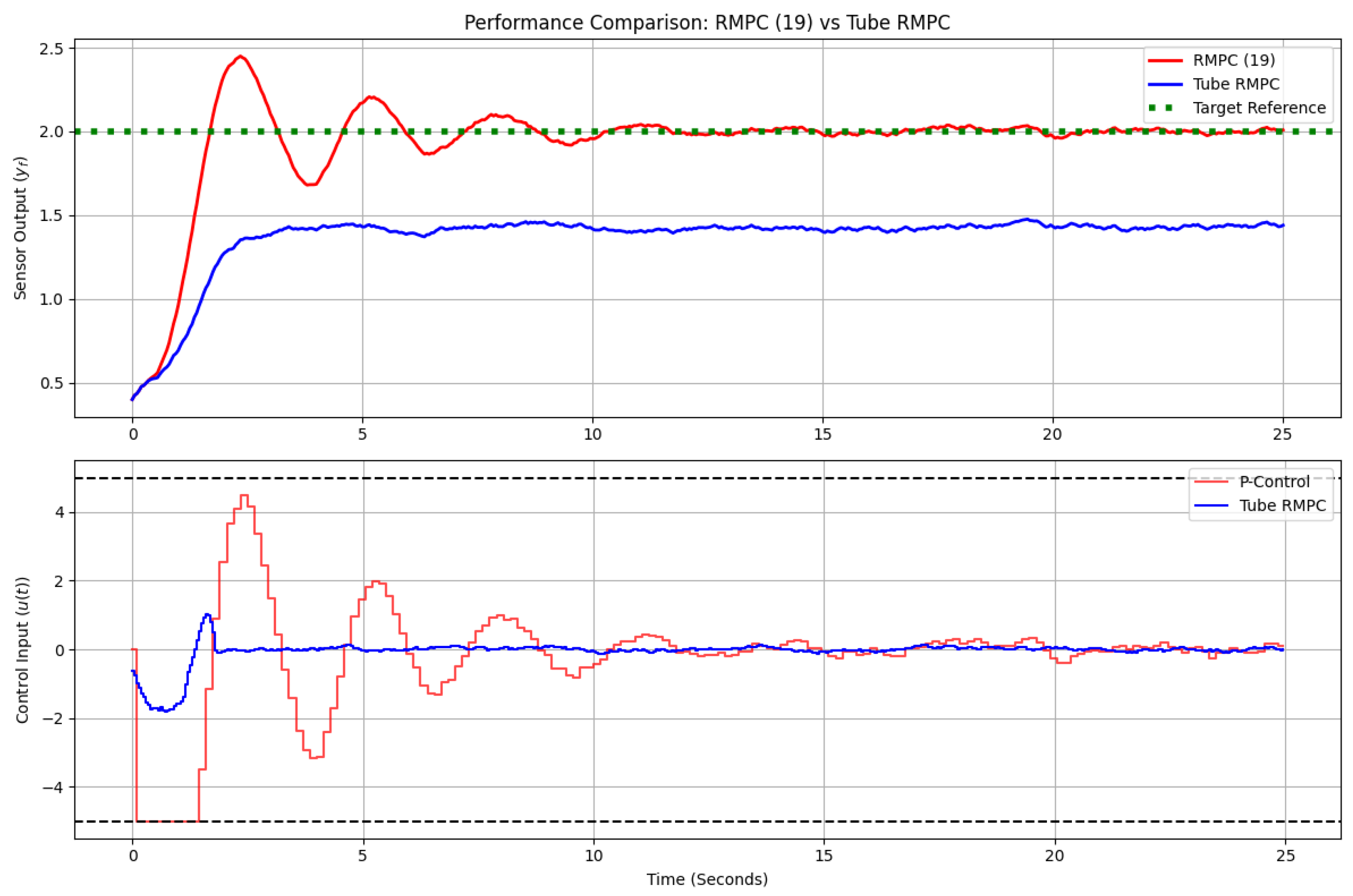
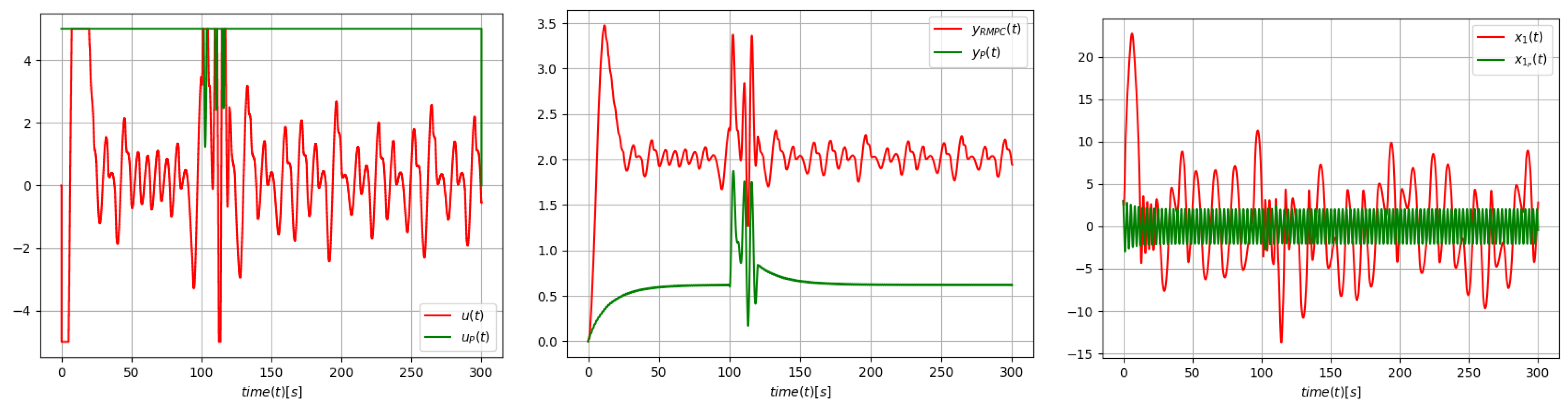
To demonstrate the efficacy of our approach, we provide a comparative analysis against the tube-based robust model predictive control (Tube-RMPC) framework proposed in [14]. In that benchmark scheme, an auxiliary feedback controller is utilized to tightly constrain the actual system states within a robust invariant "tube" centered around a prescribed nominal trajectory. For a rigorous evaluation, a bounded environmental noise characterized by a uniform distribution is introduced, and the control input constraint is set to $u_{\max }=5$. The corresponding simulation results are presented in Figure 9. To establish a quantitative performance comparison, the mean absolute error (MAE), defined as

$$\mathrm{MAE}={\displaystyle \frac{1}{N}}{\displaystyle \sum _{k=0}^{N-1}}|y\left(k\right)-y_{\mathrm{ref}}\left(k\right)|,$$

is evaluated. Our proposed approach achieves an MAE of $4.09\times {10}^{-2}$, significantly outperforming the Tube-RMPC framework in [14], which yields an error of $6.31\times {10}^{-1}$. This stark contrast clearly evidences the architectural and tracking advantages of our proposal.

Notice that a sign function is used on the internal variable z(t) to preserve the correlation between signals. To test whether the proposed framework destroys the actuator, the Total Variation (TV) of the control input:

$$\mathrm{TV}={\displaystyle \sum _{k=0}^{n-1}}|u(k+1)-u\left(k\right)|$$

is evaluated, where a high TV directly correlates with reduced actuator lifetime. We obtain $\mathrm{TV}=117$ in our case versus $\mathrm{TV}=246$ in the Tube-RMPC approach, demonstrating a drastic reduction in $\mathrm{TV}$. Finally, Appendix A presents a comparison with a standard proportional control, illustrating the improvements achieved by our framework.

6. Engineering Applications

The robust model predictive control strategy developed in this work is applicable to a wide range of engineering systems exhibiting inverse proportional or inverse-response dynamics. Such behavior is frequently encountered in practical systems where an increase in the control input produces a reduction in the measured output, leading to control challenges when conventional feedback strategies are employed. A primary application domain is sensor systems and signal conditioning circuits. Many electronic, electromechanical, and impedance-based sensors exhibit inverse response characteristics, particularly when frequency-modulated or oscillator-based measurement principles are used. The proposed control approach enables stable regulation of such systems while attenuating oscillatory behavior, making it suitable for precision sensing and calibration tasks. The method is also relevant to voltage-controlled oscillators and oscillator-based systems, which are widely used in communication, measurement, and sensing applications. Since the Van der Pol oscillator provides a representative mathematical model for such devices, the proposed inverse proportional system and its associated control law can be employed for the real-time stabilization and tuning of oscillator-driven platforms. Another important application concerns embedded and low-cost digital control systems. The explicit nature of the derived RMPC law eliminates the need for online optimization, terminal constraints, or complex numerical solvers. Consequently, the controller can be readily implemented on microcontrollers, digital signal processors, or field-programmable gate arrays, making it attractive for industrial and real-time applications with limited computational resources. In process control and industrial automation, inverse response dynamics are common in thermal, chemical, and fluid systems, where delays, competing physical effects, or nonlinearities are present. The proposed RMPC framework provides a robust alternative to classical PID-based approaches, offering improved stability and disturbance rejection without requiring detailed high-order plant models. Finally, due to its analytical transparency and low implementation complexity, the proposed control strategy is suitable for educational, experimental, and rapid-prototyping environments. It can serve as a practical example of robust predictive control applied to nonlinear systems, facilitating controller design, testing, and validation in laboratory-scale setups.

7. Conclusions

In this study, we developed a suboptimal Robust Model Predictive Control framework specifically tailored for inverse-proportional systems, utilizing a realization based on the Van der Pol oscillator. Since the VDP is a well-established system suitable for electronic implementation, the proposed inverse-proportional structure is highly amenable to laboratory validation. Furthermore, while physical implementation is identified as a priority for future work, the explicit nature of the derived suboptimal RMPC algorithm confirms its potential for realization on low-cost digital microprocessors or FPGAs. As established in Theorem 1, our framework yields a simplified control law that effectively stabilizes a nonlinear third-order system while obviating the necessity for terminal constraints or complex online optimization. Numerical simulations rigorously validated the efficacy of this design, with disturbance-rejection experiments demonstrating that stable reference tracking is maintained even in the presence of external perturbations. This underscores the framework’s potential for industrial and process control applications characterized by inverse dynamics.