A Dual-Stream Late-Fusion CNN-LSTM with Adaptive Gated Shortcut for Traffic Flow Prediction

Abstract

Traffic flow prediction is important for route planning, signal control, and traffic guidance. However, traffic-state sequences usually exhibit non-stationarity, periodicity, and complex temporal dependencies, which makes it difficult for traditional statistical methods and single deep learning models to simultaneously capture short-term local fluctuations and long-term evolutionary trends. To address this issue, this paper proposes a dual-stream latefusion CNN-LSTM with an adaptive gated shortcut for traffic flow prediction, denoted as AGS-CNN-LSTM. The proposed method does not aim at explicit spatial-topology modeling; instead, it focuses on improving the fusion mechanism of CNN-LSTM-based models under settings without graph-structure constraints. Based on two public datasets, PeMS-BAY and PeMSD8, this study constructs multi-step prediction tasks with horizons of 15 min, 30 min, 60 min, 90 min, and 120 min and compares the proposed model with MLP, SimpleRNN, 1DCNN, LSTM, Serial CNN-LSTM, CNN-LSTM-Attention, BiLSTM-Attention, TCN-LSTM, Transformer Encoder, DLinear, and DS-CNN-LSTM (w/o Gate). The experimental results show that AGS-CNN-LSTM does not consistently achieve the best performance across all datasets, prediction horizons, and evaluation metrics. Nevertheless, it performs close to the best baseline models on the 30 min and 60 min tasks of PeMS-BAY and achieves competitive RMSE and R² results on the 15 min, 30 min, and 60 min tasks of PeMSD8. Further ablation experiments indicate that the adaptive gated shortcut can enhance the predictive capability of the dual-stream late-fusion structure in some scenarios, although its benefits are dependent on the dataset and prediction horizon. Overall, the proposed model is more appropriately regarded as a lightweight fusion-mechanism improvement for CNN-LSTM-based models under settings without explicit graph-structure constraints, rather than a comprehensive replacement for complex graph neural networks, Transformerbased models, or models incorporating multiple external factors. Therefore, the findings should be interpreted as proof-of-concept evidence for a lightweight CNN-LSTM fusion enhancement under constrained non-graph-input settings, rather than as evidence of broad generalizability in complete road-network-level traffic forecasting.

1. Introduction

With the continuous growth of urban traffic demand and the increasing complexity of road networks, traffic congestion has become one of the key factors affecting the operational efficiency of cities [1,2]. Accurate prediction of future traffic states can provide decision support for applications such as route planning, signal control, and traffic guidance [3]. However, traffic flow is jointly influenced by various uncertain factors, and its evolution process usually exhibits non-stationarity, periodicity, and complex temporal dependency characteristics, which poses significant challenges to high-precision prediction. Traditional statistical forecasting methods, such as ARIMA, often struggle to fully capture the complex evolutionary patterns of such dynamically changing and highly nonlinear traffic data, resulting in reduced prediction accuracy [4,5].

Changes in traffic states are characterized not only by temporal dependency, but also often exhibit certain local correlation patterns [6]. Among existing deep learning methods, convolutional neural networks (CNNs), owing to their local receptive fields and parameter-sharing mechanisms, are commonly used to extract local correlation patterns from traffic data [7]. Long short-term memory (LSTM) networks alleviate the gradient vanishing problem in traditional recurrent neural networks through gated structures and have been widely applied in modeling long-term dependencies in time series [8]. When LSTM is used alone for prediction, the model generally places greater emphasis on temporal dependency modeling, while its ability to characterize local correlation patterns in traffic states is relatively limited [9]. In contrast, combining CNN with LSTM makes it possible, to some extent, to simultaneously capture local variation features and temporal dependency information, thereby providing a feasible approach for modeling complex traffic flow dynamics [10]. Therefore, the combination of CNN and LSTM, as well as their variants, has become a common research direction in traffic flow prediction. To summarize the progress in this area,

Table 1. Deep Learning-Based traffic flow prediction studies in the past five years.

Deep Learning Model	Representative Literature	Core Idea	Main Limitation	Relationship to This Paper
Pure time-series models	Bi et al. [11]	Use structures such as TCN and LSTM to model historical sequence variations.	Insufficient consideration of node propagation relationships and topology constraints.	Provides a basic reference for temporal dependency modeling in this paper.
CNN-LSTM hybrid models	Jiang et al. [12]	Use CNN to extract local patterns and LSTM to model temporal dependencies.	Mostly adopt serial or fixed fusion strategies.	This paper further improves the fusion mechanism of CNN-LSTM.
Attention-enhanced models	Topilin et al. [13]	Highlight key time steps or features through attention mechanisms.	Focus more on weight allocation, with insufficient direct supplementation of recent states.	This paper selects CNN-LSTM-Attention and BiLSTM-Attention as attention-enhanced baselines.
Graph-structured models	Su et al. [14]	Characterize spatial relationships among nodes through adjacency matrices or graph convolution.	Rely on road-topology priors and have relatively high model complexity.	This paper focuses on scenarios without explicit topology constraints.
Transformer/long-sequence models	Wen et al. [15]	Model long-range dependencies through self-attention mechanisms.	Have relatively large parameter scales and high training costs.	This paper selects Transformer Encoder as a self-attention-based sequence modeling baseline.
External-factor fusion models	Wang et al. [10]	Fuse external variables such as weather and holidays.	Depend on additional data and involve more complex input conditions.	This paper uses only historical traffic sequences.
Dynamic graph models	Shao et al. [16]	Adaptively learn dynamic relationships among nodes.	Computationally complex and costly to deploy.	Future research may extend the proposed method by combining it with dynamic graph mechanisms.
Linear decomposition models	Zeng et al. [17]	Perform time-series prediction by decomposing the sequence into trend and residual components.	Limited capability in characterizing strongly nonlinear fluctuations.	This paper selects DLinear as a lightweight time-series baseline.

reviews representative deep learning-based studies on traffic flow prediction published over the past five years.

In recent years, graph-structured spatiotemporal forecasting models have received increasing attention in traffic prediction. Bui et al. reviewed spatiotemporal graph neural networks for traffic prediction and pointed out that such models usually use graph structures to characterize spatial dependencies in traffic networks while combining temporal modeling modules to capture the dynamic evolution of traffic states [18]. Jiang and Luo further summarized the applications of graph neural networks in traffic flow prediction, speed prediction, and travel-demand prediction, demonstrating that GNNs have become an important research direction in traffic prediction [19]. In terms of specific models, DCRNN-type methods usually model traffic propagation as a diffusion process on a directed graph, thereby capturing directional propagation relationships in road networks [20]. STGCN-type methods jointly extract spatial and temporal dependencies through graph convolution and temporal convolution, and recent studies have further developed dynamic adaptive spatiotemporal graph convolutional structures [21]. ASTGCN-type methods introduce spatial attention and temporal attention mechanisms on the basis of graph convolution to highlight the influence of key nodes and key time intervals on prediction results [22]. Graph WaveNet-type methods learn potential node relationships through adaptive adjacency matrices and combine dilated causal convolution to enhance temporal modeling capability [23]. In addition, some studies have combined Transformers with graph convolutional networks to improve the modeling of long-range spatiotemporal dependencies [24]. However, these graph-based spatiotemporal models usually require complete road topology, adjacency matrices, node-distance matrices, or multi-node graph structures as input, and their model structures and training costs are relatively high. Different from such explicit spatial-topology modeling methods, the current experiments in this paper do not introduce road adjacency matrices or graph-structure constraints, but instead focus on improving the internal fusion mechanism of CNN-LSTM-based models under historical traffic-state sequence inputs. Therefore, the proposed model is not positioned as a comprehensive replacement for complex spatiotemporal models such as DCRNN, STGCN, ASTGCN, Graph WaveNet, or graph Transformers. Rather, it is regarded as a lightweight fusion-mechanism improvement under settings without explicit topology input.

As shown in Table 1, existing traffic prediction methods can be broadly divided into sequence modeling methods and complex spatiotemporal modeling methods. Sequence modeling methods are relatively simple in structure, but their feature-fusion strategies are often fixed, making it difficult to dynamically coordinate local fluctuations, temporal dependencies, and recent-state information under different traffic conditions. Graph-structured models, attention-based models, and Transformer-based models have stronger representation capabilities, but they usually rely on road topology, additional input information, or higher computational costs. It should be emphasized that traffic prediction generally has clear spatiotemporal characteristics, and complete road-network-level forecasting tasks need to consider both temporal evolution and spatial interactions among road nodes. This paper does not position the proposed model as a complete spatiotemporal graph forecasting model, nor does it attempt to replace topology-aware methods such as DCRNN, STGCN, ASTGCN, Graph WaveNet, or graph Transformers. Instead, it focuses on improving the internal fusion mechanism of CNN-LSTM-based models using only historical traffic-state sequences when reliable adjacency matrices, node-distance matrices, or external factors are unavailable.

Based on the above analysis, three research gaps remain to be further addressed. First, traditional statistical methods and single deep learning models still have difficulty simultaneously capturing random short-term fluctuations and evolutionary trends over longer time scales. Second, existing CNN-LSTM-based methods mostly adopt serial structures or fixed fusion strategies, which insufficiently model the coordination among local variation features, temporal dependency features, and recent-state information. Third, although complex graph models, Transformer-based models, and external-factor-fusion models have strong representation capabilities, they are not always applicable in scenarios where only historical traffic-state sequences are available. Therefore, constructing a lightweight fusion structure that can coordinate local fluctuations, temporal dependencies, and recent-state information under settings without explicit road-topology input is the core research gap that this paper aims to bridge.

Accordingly, the objective of this study is not to construct a complete topology-aware spatiotemporal forecasting framework, but to examine whether the internal fusion mechanism of CNN-LSTM-based models can be improved when only historical traffic-state sequences are available. Under this constrained non-graph-input setting, AGS-CNN-LSTM is designed as a lightweight fusion-mechanism enhancement rather than a universal traffic forecasting architecture. Its contribution should therefore be understood as an incremental structural optimization of CNN-LSTM information fusion, rather than as a fundamentally new traffic forecasting paradigm.

The main contributions of this paper are summarized as follows:

1.

A parallel dual-stream late-fusion CNN-LSTM framework is proposed. Different from the conventional serial CNN-LSTM structure, which performs convolutional modeling followed by recurrent modeling in a fixed order, the proposed framework arranges 1D-CNN and LSTM as parallel branches. These two branches separately extract local correlation patterns and temporal evolution features from the input sequence and then jointly represent them in the late-fusion stage. This structure aims to reduce the restriction caused by sequential information transmission through a single path, allowing local fluctuation information and temporal dependency information to participate in prediction in a relatively independent and complementary manner.

2.

An adaptive gated shortcut mechanism based on a recent-state anchor is designed. This mechanism directly introduces the observation at the last time step of the input sequence as recent-state information near the prediction starting point. A dynamic gate is then generated from the deep features fused by CNN-LSTM to adaptively regulate the contribution of this recent-state information to the final prediction. Compared with ordinary residual connections or fixed fusion strategies, this mechanism does not simply transmit intermediate hidden features. Instead, it uses deep fused features to dynamically determine whether the raw observation at the end of the input sequence should participate in the final prediction, thereby establishing an adjustable information-supplementation channel between deep historical representations and the recent raw state.

3.

The proposed model is evaluated on two public datasets, PeMS-BAY and PeMSD8, under five prediction horizons: 15 min, 30 min, 60 min, 90 min, and 120 min. The comparison models include Serial CNN-LSTM, CNN-LSTM-Attention, BiLSTM-Attention, TCN-LSTM, Transformer Encoder, DLinear, and DS-CNN-LSTM (w/o Gate). These comparisons are used to analyze the competitiveness and applicability boundary of the proposed model across different prediction horizons.

2. Methodology

To address the complex nonlinear dependency relationships in traffic flow sequences, this study develops a dual-stream late-fusion CNN-LSTM model with an adaptive gated shortcut (AGS-CNN-LSTM) for multi-step traffic state prediction. In recent years, deep learning methods have been widely applied in the field of intelligent transportation, and the combination of CNN and LSTM, in particular, has shown good applicability in modeling local variations and capturing temporal dependencies [25,26]. However, most existing methods adopt relatively fixed feature fusion strategies, making it difficult to fully balance short-term local variation information and long-term evolutionary trends when traffic states fluctuate. To this end, a parallel dual-stream structure is designed in this study to extract different types of features separately, and an adaptive gated shortcut mechanism is introduced to regulate the fusion process, thereby enhancing the model’s adaptability to different traffic states.

2.1. Overall Architecture

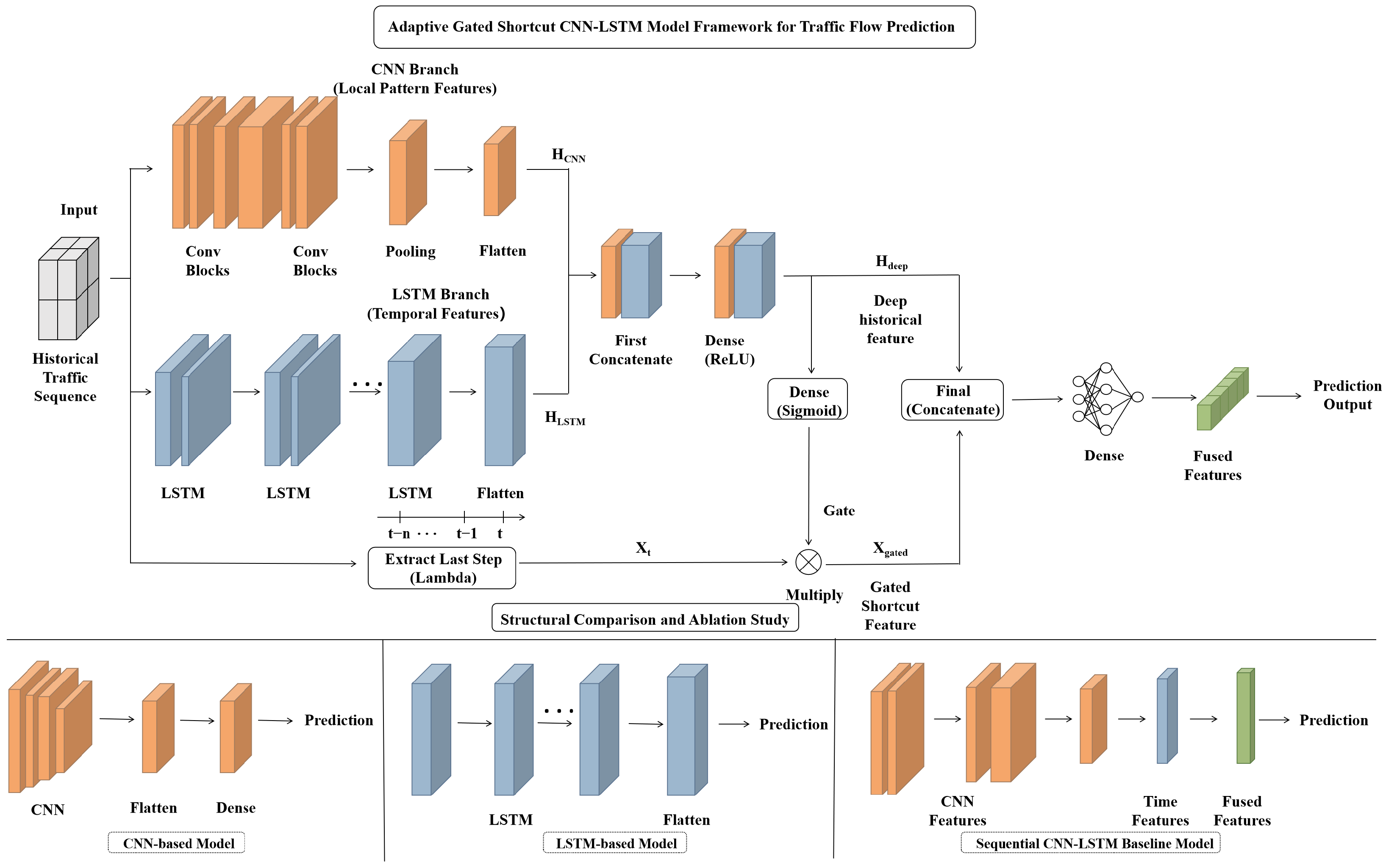
The overall architecture of AGS-CNN-LSTM is shown in Figure 1, which consists of an input layer, parallel feature extraction branches, an adaptive gated fusion module, and a prediction output layer.

Let the normalized historical traffic flow sequence be denoted as $X\in {\mathbb{R}}^{B\times K\times F}$, where B denotes the batch size, K denotes the number of historical observation time steps, F denotes the input feature dimension. For PeMS-BAY, $F=1$; for PeMSD8, $F=170$.

The input sequence X is fed into two parallel branches simultaneously. The CNN branch is used to extract local correlation features within a short time range, while the LSTM branch is used to model the dynamic evolution of the time series. Compared with a serial structure, the parallel design avoids sequential feature transmission through a single path and, to some extent, reduces the influence of intermediate transformations on the original temporal information. On this basis, the model jointly models the deep fused features and current-state information through the adaptive gated shortcut mechanism, and finally outputs the predicted traffic state at the specified prediction horizon.

To further clarify the input and output dimensions of different datasets and the tensor flow among different modules,

Table 2. Main tensor dimensional flow in AGS-CNN-LSTM.

Module	Operation	PeMS-BAY Tensor Shape	PeMSD8 Tensor Shape	Description
Input	Historical window	$(B\times K\times 1)$	$(B\times K\times 170)$	Historical traffic-state input
CNN branch	Conv1D + pooling + flatten	$(B\times d_c)$	$(B\times d_c)$	Extraction of short-term local variation features
LSTM branch	LSTM hidden output	$(B\times d_l)$	$(B\times d_l)$	Extraction of temporal dependency features
Late fusion	Concatenation	$(B\times (d_c+d_l))$	$(B\times (d_c+d_l))$	Fusion of dual-stream features
Dense mapping	Fully connected layer	$(B\times d_h)$	$(B\times d_h)$	Generation of deep fused representation
Shortcut branch	Last input step	$(B\times 1)$	$(B\times 170)$	Raw observation at the end of the input sequence
Gate	Sigmoid gate	$(B\times 1)$	$(B\times 1)$	Generation of gate weights from deep fused features
Gated shortcut	Element-wise modulation	$(B\times 1)$	$(B\times 170)$	Regulation of the contribution of the recent-state anchor
Final fusion	Concatenation	$(B\times (d_h+1))$	$(B\times (d_h+170))$	Fusion of deep features and shortcut features

presents the main tensor dimensional changes of AGS-CNN-LSTM under the PeMS-BAY and PeMSD8 experimental settings. Here, B denotes the batch size, and K denotes the length of the historical observation window. In the main experiments of this paper $K=12$.

As shown in Table 2, the PeMS-BAY experiment corresponds to a single-sensor traffic speed prediction task; therefore, both the input and output are univariate. In contrast, the PeMSD8 experiment corresponds to a multi-node single-channel traffic flow prediction task involving 170 monitoring sensors; therefore, the model outputs the traffic flow values of all nodes at the specified prediction horizon. Although the two tasks differ in terms of input and output dimensions, they follow the same overall procedure of dual-stream feature extraction, gated shortcut modulation, and late fusion.

2.2. Parallel Extraction Branches for Local Correlation Features and Temporal Dependency Features

2.2.1. CNN-Based Local Correlation Feature Extraction

Traffic state sequences usually exhibit a certain degree of local continuity and interaction within a short time range, and adjacent time steps are often not independent of each other but instead show evident short-term response characteristics [27]. Previous studies have shown that one-dimensional convolutional neural networks (1D-CNNs), by virtue of their local receptive fields and parameter-sharing mechanisms, can effectively extract local patterns from sequences and enhance the model’s ability to represent short-term variation information [28]. Based on this, a 1D-CNN is adopted in this study to model the input sequence so as to capture the local correlation patterns among adjacent time steps.

It should be noted that, under the current experimental setting of this study, the CNN branch does not correspond to spatial-topology modeling in the strict sense. Since this paper does not introduce road adjacency matrices, node-distance matrices, or graph-structure constraints, the term “local correlation features” mainly refers to local variation relationships and neighboring response patterns among adjacent time steps in historical traffic-state sequences, rather than spatial correlations defined by road topology. The mathematical expression is as follows:

$$F_s=Flatten(MaxPool(ReLU(W_c\ast X+b_c)))$$

where $F_s$ denotes the local correlation feature vector extracted by the CNN branch, $W_c$ is the weight matrix of the convolution kernel, and $b_c$ is the bias term of the convolution operation. The symbol * represents the one-dimensional convolution operation (1D convolution). $ReLU(·)$ denotes the nonlinear activation function, and $MaxPool(·)$ represents the max-pooling operation. Through the convolution and pooling processes, this branch extracts local variation patterns from the sequence and, to a certain extent, compresses redundant information while retaining the short-term response features that are more critical for prediction.

2.2.2. LSTM-Based Temporal Feature Extraction

In addition to local variations, traffic flow data usually exhibit evident temporal dependencies and staged evolutionary characteristics [29]. By introducing an input gate, a forget gate, and an output gate, long short-term memory (LSTM) networks can alleviate, to a certain extent, the gradient vanishing problem encountered by traditional recurrent neural networks in long-sequence modeling, and have therefore been widely applied in traffic flow prediction tasks [30]. In this study, the LSTM branch is used to characterize the dynamic evolution of traffic flow over time, and its state update process at each time step can be expressed as follows:

$$F_t=LSTM(X,h_{t-1},c_{t-1})$$

where $F_t$ denotes the final temporal feature vector, and $h_{t-1}$ represents the hidden state vector at the previous time step, which is responsible for carrying historical short-term memory information. $c_{t-1}$ denotes the cell state vector at the previous time step, which is used to preserve evolutionary trends over a longer time range. Through this branch, the model is able to capture the temporal dependency relationships in traffic sequences and provide temporal semantic information for the subsequent fusion process.

2.3. Adaptive Gated Shortcut and Feature Fusion Module

It should be noted that the adaptive gated shortcut proposed in this paper is not a simple residual connection or a fixed gated fusion mechanism. A conventional residual connection is usually used to transmit intermediate hidden features in deep networks to alleviate gradient vanishing or information attenuation. In contrast, the shortcut branch in this paper directly introduces the raw observation at the last time step of the input sequence as a recent-state anchor near the prediction starting point. Meanwhile, this recent-state information is not added to the model output with a fixed weight. Instead, dynamic gate weights are generated from the deep features fused by the CNN-LSTM dual streams, so that the participation intensity of the recent-state information can be adaptively adjusted according to different traffic states. Therefore, the core function of this mechanism is to dynamically coordinate deep historical representations and current-state information, rather than simply replicating an existing residual structure.

From the perspective of structural function, the distinction of AGS-CNN-LSTM does not lie in simply stacking CNN, LSTM, and gating layers. Instead, it organizes three types of information sources through different paths: the CNN branch extracts local variation patterns among adjacent time steps within the historical window, the LSTM branch extracts longer-term temporal dependency features, and the shortcut branch directly preserves the raw observed state near the prediction starting point. The gate weights are generated from the deep representation fused by the CNN-LSTM dual streams and are used to regulate the contribution of the recent-state anchor. Therefore, this structure forms a fusion strategy of “deep historical representation-driven recent-state supplementation”, rather than a simple variant of conventional serial CNN-LSTM, ordinary late concatenation, or hidden-feature residual transmission. To further avoid misunderstanding, the recent-state anchor is not used as an independent prediction output or as the first forecasted value. Instead, it only serves as supplementary raw-state information near the prediction starting point. The final prediction is still generated by the output layer after the deep fused representation and the gated shortcut feature are concatenated. In this way, the shortcut branch provides a controllable information-supplementation path, while the gate determines the strength of this supplementation according to the deep CNN-LSTM representation. This design is not intended to claim a fundamentally new neural architecture. Rather, it provides a lightweight information-flow reorganization strategy that combines deep historical representations with a learnable recent-state supplementation path.

After obtaining the local correlation features extracted by the CNN branch and the temporal features extracted by the LSTM branch, traditional dual-stream networks usually adopt direct concatenation for feature fusion and use the fused result for final prediction [31]. However, as the prediction horizon increases, deep features may gradually deviate from the raw state information near the prediction starting point during multi-layer mapping, thereby aggravating error propagation and information attenuation in multi-step prediction [32].

For this reason, this paper introduces an adaptive gated shortcut mechanism into the dual-stream late-fusion framework to enhance the model’s ability to retain current-state information and improve the flexibility of the fusion process.

2.3.1. Initial Construction of Deep Fused Features

The local correlation features $H_{cnn}$ output by the CNN branch and the temporal features $H_{lstm}$ output by the LSTM branch are concatenated along the feature dimension and then nonlinearly mapped through a fully connected layer to further model the coupling relationship between these two types of features, thereby forming a preliminary deep fused feature representation. Compared with simple end-stage concatenation, this process can enhance, to a certain extent, the interactive representation capability between different types of features and provide more comprehensive high-level semantic information for the subsequent gating adjustment. Its mathematical expression is given as follows:

$$H_{concat}=[H_{cnn},H_{lstm}]$$

$$H_{deep}=ReLU(W_{deep}·H_{concat}+b_{deep})$$

where $[·,·]$ denotes the feature concatenation operation. $W_{deep}$ and $b_{deep}$ represent the weight matrix and bias term of the fully connected layer, respectively. $ReLU$ denotes the activation function, and $H_{deep}$ represents the preliminary deep fused feature representation.

2.3.2. Shortcut Branch Extraction and Calculation of Adaptive Gating Weights

Traffic time series usually exhibit a certain degree of short-term continuity, and future states often maintain a strong correlation with observations near the prediction starting point. In particular in multi-step prediction tasks, the observation at the end of the input sequence can, to some extent, reflect the immediate operating state around the current time. Therefore, a shortcut branch is constructed in this study to directly introduce the observation at the last time step of the input sequence as a supplementary source of current state information. It should be noted that this branch is not intended to replace deep features for independent prediction, but rather to serve as a reference anchor for recent states, so as to preserve a direct perception of the current state in addition to deep feature representation.

Considering that the role of recent observation information is not entirely consistent across different traffic states and prediction tasks, indiscriminately introducing it into the final output may instead weaken the model’s effective utilization of deep historical features. Based on this, the preliminary deep fused features are further used in this study to generate dynamic gating weights, so as to adaptively regulate the contribution of the shortcut branch. The calculation process is given as follows:

$$Gate=\sigma (W·H_{deep}+b_{gate})$$

where $\sigma$ denotes the Sigmoid activation function, which constrains the gating weights to the range of $(0,1)$. $W_{gate}$ and $b_{gate}$ are the learnable parameters of the gating fully connected layer.

The gating variable is generated under the guidance of the deep fused features, and its role is to adaptively regulate the degree of participation of the shortcut information according to the current input state, thereby enabling the model to more flexibly balance the relative contributions of recent observation information and deep historical representations.

From the mathematical intuition, the deep fused feature $H_{deep}$ can be regarded as a high-level temporal pattern representation extracted from the entire historical window, while the observation $x_t$ at the end of the input sequence provides a recent-state anchor near the prediction starting point. For traffic states with strong short-term continuity, the future target usually remains highly correlated with $x_t$. However, for samples with drastic fluctuations or longer prediction horizons, excessive reliance on $x_t$ may introduce short-term state bias. Therefore, this paper uses $H_{deep}$ to generate the gate weight g, and applies $g\odot x_t$ to adaptively regulate the recent-state information for each sample. When the deep historical features indicate that the recent state has high reference value, the gate weight can enhance the contribution of the shortcut branch. When the relationship between the recent state and the future target weakens, the gate weight can reduce its influence. This design enables the model to dynamically balance deep historical representations and the recent raw state.

2.3.3. Gated Modulation and the Late-Fusion Framework

After the gating weights are obtained, they are multiplied element-wise with the residual shortcut $X_t$ to produce the adaptively modulated shortcut feature $X_{gated}$. Subsequently, the modulated shortcut feature is concatenated again with the deep fused feature $H_{deep}$ and the resulting representation is fed into the final output layer to obtain the prediction results:

$$X_{gated}=Gate\otimes X_t$$

$$H_{final}=[H_{deep},X_{gated}]$$

$$\hat{Y}=W_{out}·H_{final}+b_{out}$$

where ⊗ denotes element-wise multiplication. $W_{out}$ and $b_{out}$ are the parameters of the output layer. $\hat{Y}$ denotes the traffic-state value finally predicted by the model at the specified prediction horizon.

Through the above design, AGS-CNN-LSTM achieves the collaborative utilization of deep historical features and current state information within a unified framework. For samples with relatively stable traffic states and strong short-term continuity, the gated shortcut can provide effective supplementary recent-state information for the model. In contrast, when traffic state changes are more complex or the prediction horizon is longer, the model relies more on the deep fused features to complete the prediction. Overall, this module is intended to provide a more flexible fusion strategy for the joint modeling of local correlation features and temporal dependency features, and to alleviate, to some extent, the problem of information attenuation in multi-step prediction.

3. Experimental Setup and Model Architecture

3.1. Experimental Data Processing

3.1.1. Description of the Experimental Datasets

To evaluate the applicability of the proposed model in different traffic scenarios, this paper selects two public traffic datasets, PeMS-BAY and PeMSD8, for experiments. Both datasets are derived from the California Department of Transportation Performance Measurement System (Caltrans PeMS) and have good data continuity and practical application backgrounds. The temporal resolution of both datasets is 5 min, meaning that each day contains 288 consecutive time steps. Considering that the two datasets differ in file format, node scale, and input organization, this paper constructs prediction tasks separately according to their data characteristics.

The PeMS-BAY dataset is stored in CSV format. After reading the CSV file, this paper selects the first data column after the time-index column as the modeling object and constructs a single-sensor traffic speed prediction task. The current experiment uses the complete available time series in the CSV file, containing 52,116 time steps.

The PeMSD8 dataset is stored in .npz format, and its core data array can be represented as a three-dimensional tensor “$T\times N\times C$”, where “T” denotes the number of time steps, “N” denotes the number of traffic monitoring sensors, and “C” denotes the number of traffic-state feature channels. The original PeMSD8 data used in this paper have a dimension of $17,856\times 170\times 3$, the 0-th feature channel is selected as the prediction object, and the continuous observations of all 170 monitoring sensors under this channel are retained. To control the computational scale of the multi-node prediction experiment, this paper extracts 14 consecutive days of data from PeMSD8 as the experimental window, namely $14\times 288=4032$ time steps. Therefore, the PeMSD8 experiment corresponds to a multi-node single-channel traffic flow prediction task, and the prediction target is the traffic flow values of all monitoring sensors at the specified future time step. Although the two datasets differ in sensor scale, input dimensionality, and prediction targets, they are processed under a unified experimental workflow, including the same historical window length, prediction horizons, chronological data-splitting strategy, training procedure, and evaluation metrics. This design is intended to ensure internal comparability among different models under constrained non-graph-input settings, rather than to claim that the two datasets represent identical traffic prediction scenarios.

It should be noted that the experimental setting of this paper has certain scope limitations. First, the PeMS-BAY experiment uses only a single monitoring sensor’s traffic speed sequence for modeling. Therefore, it mainly analyzes the performance of the proposed structure in a univariate speed sequence prediction task and cannot represent the complete PeMS-BAY road-network-level multi-node prediction task. Second, although the PeMSD8 experiment retains 170 monitoring sensors, it uses only the 0-th traffic-state channel and extracts 14 consecutive days of data for experiments. Therefore, the PeMSD8 experiment is mainly used to compare the relative performance of different models in a multi-node single-channel flow prediction task under a unified computational scale, and it is insufficient to fully reflect the generalization capability under longer time spans, multi-feature inputs, and complete road-topology constraints. Based on the above settings, the experimental conclusions of this paper should be understood as validation of a CNN-LSTM-based fusion mechanism under settings without explicit topology input, rather than as a comprehensive evaluation of a complete road-network-level spatiotemporal prediction system. Future research may further validate the proposed mechanism more systematically using complete multi-sensor PeMS-BAY data, longer PeMSD8 time spans, multi-channel traffic-state variables, and conditions where road adjacency matrices or distance matrices are available.

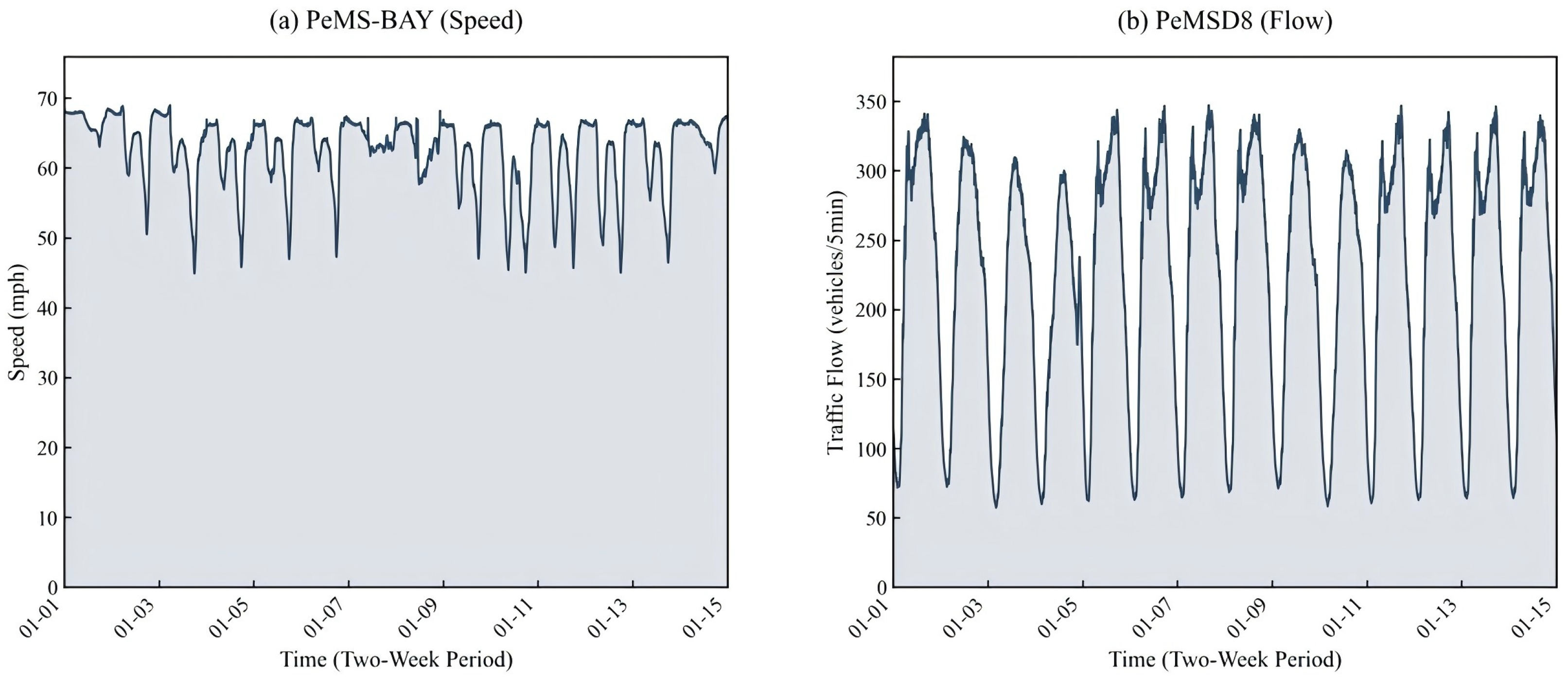
Therefore, the present experimental design should be interpreted as a proof-of-concept evaluation of the proposed fusion mechanism under constrained non-graph-input settings. It is not intended to establish full generalizability across complete road-network-level forecasting tasks, longer time spans, multi-channel traffic variables, or topologyaware scenarios. Figure 2 shows the raw traffic-state sequences used for modeling in the PeMS-BAY and PeMSD8 datasets, providing a visual comparison of their temporal variation patterns.

3.1.2. Data Preprocessing and Sample Construction

Before sample construction, this paper first conducts data quality checks on the input sequences of the two datasets, mainly including checks for missing values, infinite values, and obvious abnormal records. For the PeMS-BAY dataset, after reading the CSV file, this paper selects the traffic speed sequence used for modeling and checks whether missing values or non-numeric records exist in the sequence. For the PeMSD8 dataset, after reading the .npz file, this paper selects the 0-th feature channel from the data tensor and performs the same checks on the retained multi-node traffic flow matrix.

The data quality check results show that no NaN or Inf records affecting model training are found in the PeMS-BAY single-column speed sequence or the PeMSD8 0-th-channel multi-node flow matrix used in this paper. Therefore, no additional complex data imputation procedure is introduced. In practical applications, if continuous missing values or severe abnormal records exist, methods such as linear interpolation, historical mean imputation, or smoothing based on adjacent time steps may be further adopted for processing.

To reduce the influence of different data dimensions and value ranges on model training, this paper applies min–max normalization to the input sequences. For an original observation x, its normalized result x can be expressed as follows:

$$x={\displaystyle \frac{x-x_{min}}{x_{max}-x_{min}}}$$

where $x_{min}$ and $x_{max}$ denote the minimum and maximum values in the training data, respectively. Model training and prediction are both conducted on the normalized scale. During model evaluation, the prediction results are inverse-normalized back to the original scale, and RMSE, MAE, MAPE, and ${\mathrm{R}}^2$ are then calculated.

It should be noted that the experiments in this paper are conducted based on public PeMS datasets, and no sensors are redeployed or raw road traffic data are newly collected. The original traffic-state data are collected and released by road monitoring devices in the PeMS system. The data preparation in this paper mainly includes data field selection, continuous time-window extraction, normalization, sliding-window sample construction, and chronological splitting of the training and test sets. Therefore, the model performance is affected to some extent by the quality, missing-data conditions, and temporal continuity of the original sensor records in the public datasets. To reduce the influence of data-processing differences on model comparison, all comparison models adopt the same data preprocessing procedure, input window length, and prediction horizon settings.

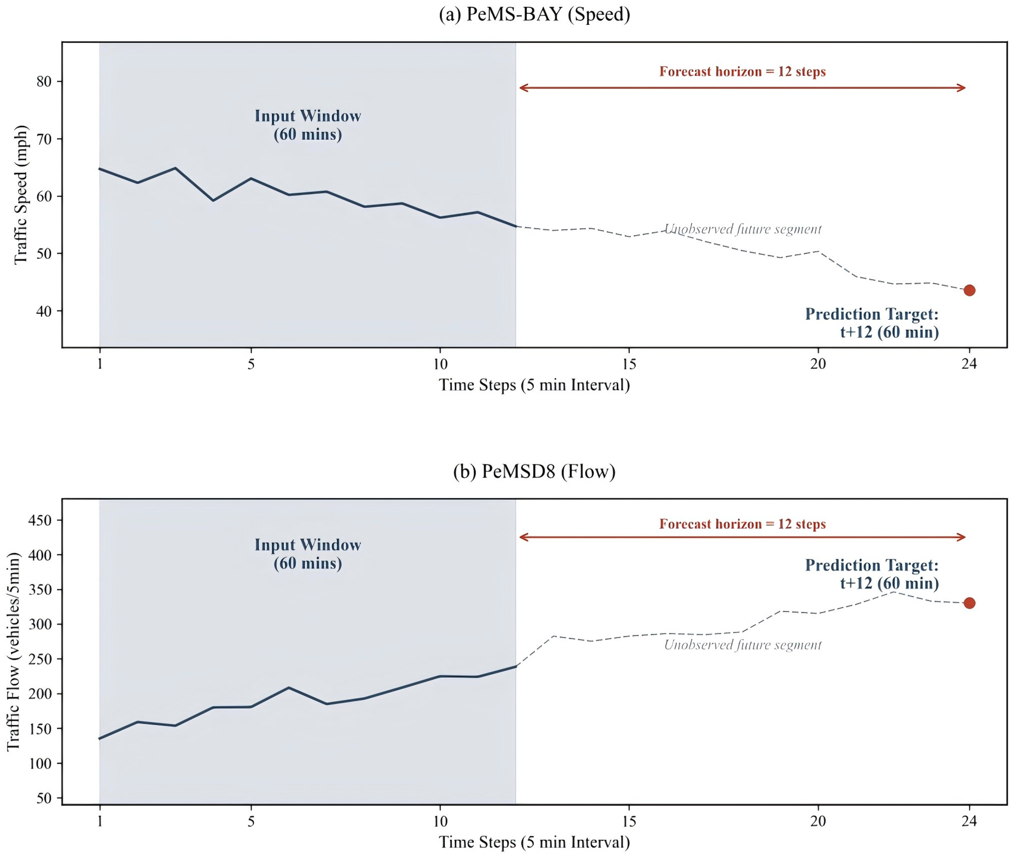
Considering that traffic time series have clear temporal dependencies, this paper constructs supervised learning samples using a sliding-window strategy. Specifically, historical observations from 12 consecutive time steps are used as the input window, while the traffic states at the future 3rd, 6th, 12th, 18th, and 24th time steps are used as prediction targets, respectively. In this way, five multi-step prediction tasks are formed, corresponding to 15 min, 30 min, 60 min, 90 min, and 120 min. During sample construction, adjacent samples slide forward by one time step. The corresponding sliding-window-based multi-step sample construction process is illustrated in Figure 3.

In terms of data splitting, after completing sliding-window sample construction, this paper uses the first 80% of samples as the training set and the last 20% as the test set in chronological order, so as to avoid temporal information leakage. During training, 10% of the training set is further used as the validation set for training monitoring and parameter adjustment. It should be noted that PeMS-BAY and PeMSD8 differ in their input organization forms, but they remain consistent in terms of window length, prediction horizons, chronological splitting strategy, and training procedure. Therefore, this paper places greater emphasis on the consistency of the two experiments in sample construction logic and experimental workflow, rather than simply treating them as completely identical input settings.

To further clarify the transformation relationship from raw data to model input,

Table 3. Description of the data structures for model inputs and prediction targets.

Dataset	Raw Data Format	Selected Variable	Used Time Steps	Input Sample (X)	Prediction Target (y)	Task Type
PeMS-BAY	CSV	The first traffic speed column after the time index	52,116	$X\in {\mathbb{R}}^{K\times 1}$$K=12$	$(y_{t+H}\in {\mathbb{R}}^1)$	Single-sensor speed prediction
PeMSD8	.npz data tensor	Channel 0 of all 170 sensors	4032	$X\in {\mathbb{R}}^{K\times 170}$$K=12$	$(y_{t+H}\in {\mathbb{R}}^{170})$	Multi-node single-channel flow prediction

summarizes the input organization forms and prediction targets of the two datasets in the experiments of this paper. It can be seen that PeMS-BAY and PeMSD8 differ in raw data format, number of sensors, and output dimension. However, both datasets use a historical observation window of length K = 12 to construct supervised learning samples and are evaluated for multi-step prediction under the same prediction horizon settings.

3.2. Network Configuration and Model Parameter Settings

To ensure the comparability among different models, all experiments in this study are implemented under a unified software environment and follow the same data preprocessing procedure, sample partitioning strategy, loss function form, and training workflow. For both the PeMS-BAY and PeMSD8 experiments, the random seed is fixed at 42 to minimize, as much as possible, the influence of random initialization on fluctuations in the experimental results.

In terms of model configuration, a parallel dual-stream structure is adopted in this study to extract local variation features and temporal dependency features separately. The convolutional branch is used to model local patterns in the input sequence, while the LSTM branch is employed to characterize the temporal evolution of traffic states. The outputs of the two branches are mapped through fully connected layers and then fused in the late stage. For the proposed AGS-CNN-LSTM model, an adaptive gated shortcut is further introduced during the fusion stage to supplement the state information at the end of the input sequence. The relevant network structural parameters and training hyperparameters are listed in

Table 4. Comparison of key hyperparameter settings.

Parameter Category	Parameter Name	Values
Input and Prediction Settings	Historical Observation Window Size (K)	12
	Prediction Horizon (H)	3, 6, 12, 18, 24
Local Correlation Feature Branch (CNN)	Kernel Size	3
	Number of Filters	64
	Activation Function	ReLU
	Pooling Window Size	2
Temporal Branch (LSTM)	Number of Hidden Units	64
	Activation Function	tanh
Feature Fusion and Gating	Neurons in the Dimensionality Reduction Fully Connected Layer	32
	Activation function for fusion layer	ReLU
	Adaptive gating network activation function	Sigmoid
Global Training Parameters	Optimizer	Adam
	Initial Learning Rate	0.001
	Batch Size	128

.

With regard to the training strategy, the mean squared error (MSE) loss function is uniformly adopted, together with an early stopping strategy and an adaptive learning rate decay mechanism, so as to improve the stability of the training process to a certain extent and reduce the risk of overfitting. It should be noted that the parameter settings in Table 4 are not only used for the proposed model but also serve as unified reference configurations for the comparative experiments of all baseline models, thereby improving the comparability of the experimental results.

3.3. Model Complexity and Computational Cost Analysis

In addition to prediction accuracy, model complexity is also an important factor for the practical deployment of traffic prediction models. To analyze the computational cost of AGS-CNN-LSTM, this paper selects several representative models, including LSTM, Serial CNN-LSTM, CNN-LSTM-Attention, TCN-LSTM, DS-CNN-LSTM (w/o Gate), and AGS-CNN-LSTM and reports their number of trainable parameters, average training time per epoch, and inference time per test sample. Since the model structure and historical input window length remain unchanged under different prediction horizons, the number of model parameters is mainly determined by the network structure, input dimension, and output dimension, rather than directly varying with the prediction horizon. Therefore, the 60 min prediction task is selected as a representative setting for complexity comparison. Training time and inference time are measured under the same experimental environment and are reported as the mean ± standard deviation over three random seeds. The results are shown in

Table 5. Comparison of model complexity and computational cost.

Dataset	Model	Parameters	Training Time/Epoch (s)	Inference Time/Sample (ms)
PeMS-BAY	LSTM	21,121	$1.441\pm 0.009$	$0.0420\pm 0.0033$
	Serial CNN-LSTM	35,393	$1.329\pm 0.023$	$0.0396\pm 0.0006$
	CNN-LSTM-Attention	37,441	$2.135\pm 0.031$	$0.0488\pm 0.0008$
	TCN-LSTM	60,097	$2.681\pm 0.006$	$0.0588\pm 0.0009$
	DS-CNN-LSTM (w/o Gate)	33,665	$1.644\pm 0.013$	$0.0463\pm 0.0005$
	AGS-CNN-LSTM	33,699	$1.675\pm 0.018$	$0.0483\pm 0.0008$
PeMSD8	LSTM	75,370	$0.569\pm 0.034$	$0.8204\pm 0.2052$
	Serial CNN-LSTM	73,418	$0.563\pm 0.018$	$0.8022\pm 0.1912$
	CNN-LSTM-Attention	75,466	$0.603\pm 0.032$	$0.9165\pm 0.0263$
	TCN-LSTM	98,122	$0.680\pm 0.022$	$0.8815\pm 0.0735$
	DS-CNN-LSTM (w/o Gate)	114,954	$0.592\pm 0.034$	$0.7860\pm 0.1292$
	AGS-CNN-LSTM	143,887	$0.597\pm 0.014$	$0.7149\pm 0.0309$

.

As shown in Table 5, in the PeMS-BAY single-sensor traffic speed prediction task, AGS-CNN-LSTM has 33,699 parameters, which is only 34 more than the 33,665 parameters of DS-CNN-LSTM (w/o Gate). Its average training time per epoch increases from 1.644 s to 1.675 s, and its inference time per sample increases from 0.0463 ms to 0.0483 ms. These results indicate that, in the univariate traffic speed prediction task, the adaptive gated shortcut introduces almost no significant increase in model parameters or inference cost, and its additional computational overhead is relatively small.

In the PeMSD8 multi-node traffic flow prediction task, because the model needs to output the predicted values of 170 monitoring sensors simultaneously, the number of parameters of AGS-CNN-LSTM increases from 114,954 for DS-CNN-LSTM (w/o Gate) to 143,887. This increase mainly comes from the additional weights introduced when the recent-state anchor and deep fused features jointly participate in the final output mapping. Nevertheless, the average training time per epoch of AGS-CNN-LSTM is 0.597 s, which is almost at the same level as the 0.592 s of DS-CNN-LSTM (w/o Gate), and the inference time per sample also remains within a similar range. This indicates that, in the multi-node prediction task, although the adaptive gated shortcut brings a certain increase in parameters, it does not significantly increase the training or inference time cost.

Compared with TCN-LSTM, AGS-CNN-LSTM has fewer parameters and a shorter training time on PeMS-BAY. On PeMSD8, AGS-CNN-LSTM has more parameters than TCN-LSTM, but its training time remains comparable.

Overall, compared with the ungated dual-stream structure, AGS-CNN-LSTM introduces only a limited number of additional parameters, while its training and inference times remain at a similar level. These results suggest that, under the current experimental setting, the adaptive gated shortcut is a lightweight structural improvement with controllable computational cost.

3.4. Experimental Setup

To improve the reproducibility of the experimental results, this paper further supplements the experimental running environment and implementation details.

Table 6. Experimental environment and implementation details.

Item	Setting
Programming language	Python 3.12
Deep learning framework	TensorFlow 2.13.2/Keras 3.13.2
Operating system	Windows 11
CPU	12th Gen Intel(R) Core(TM) i9-12900H (2.50 GHz)
GPU	CPU-only
Memory	16 GB
Random seed	42
Data splitting	Chronological split: 80% training set and 20% test set
Validation set setting	10% of the training set
Early stopping	patience = 12, restore best weights
Learning-rate decay	ReduceLROnPlateau, factor = 0.5, patience = 4

presents the software environment, hardware environment, and main training implementation settings used in the experiments. It should be noted that Table 4 is mainly used to describe the model structural parameters and training hyperparameters, whereas Table 6 mainly describes the experimental running environment; therefore, the two tables have different focuses.

3.5. Performance Evaluation Metrics

To comprehensively evaluate the performance of the models in traffic prediction tasks, this paper selects root mean square error (RMSE), mean absolute error (MAE), mean absolute percentage error (MAPE), and the coefficient of determination ${\mathrm{R}}^2$ as evaluation metrics. Among them, RMSE is more sensitive to larger errors, MAE is used to characterize the average absolute level of prediction errors, MAPE reflects the relative proportion of prediction errors with respect to the true values, and ${\mathrm{R}}^2$ is used to measure how well the model fits the variation trend of the real data. The closer ${\mathrm{R}}^2$ is to 1, the stronger the model’s ability to explain the trend. For RMSE, MAE, and MAPE, smaller values indicate better prediction performance. For ${\mathrm{R}}^2$, larger values indicate better model fitting performance. The formulas for these evaluation metrics are as follows:

$$RMSE=\sqrt{{\displaystyle \frac{1}{N}}\sum _{i=1}^N(y_i-{\hat{y}}_i{)}^2}$$

$$MAE={\displaystyle \frac{1}{N}}{\displaystyle \sum _{i=1}^N}|y_i-{\hat{y}}_i|$$

$$MAPE={\displaystyle \frac{100\%}{N}}{\displaystyle \sum _{i=1}^N}\left|{\displaystyle \frac{y_i-{\hat{y}}_i}{y_i}}\right|$$

$$R^2=1-{\displaystyle \frac{{\sum }_{i=1}^N(y_i-{\hat{y}}_i{)}^2}{{\sum }_{i=1}^N(y_i-\overline{y}{)}^2}}$$

where $y_i$ denotes the true traffic-state value of the i-th sample, ${\hat{y}}_i$ denotes the predicted value of the model, $\overline{y}$ denotes the mean value of the true observations, and N denotes the total number of samples in the test set.

3.6. Baseline Model Comparison Settings

To more objectively evaluate the performance of the proposed AGS-CNN-LSTM model in traffic time-series prediction tasks, this paper selects various basic models, hybrid-structure models, and strong temporal baseline models as comparison methods and conducts tests under a unified experimental setting. Specifically, this paper calculates the traffic-state prediction errors of each model under five prediction horizons, namely 15 min, 30 min, 60 min, 90 min, and 120 min, to compare the performance differences among different models in multi-step prediction tasks. Considering that the focus of this study is the collaborative modeling of local correlation features, temporal dependency features, and recent-state information under settings without explicit graph-structure input, the selected baseline models mainly cover several representative categories, including feedforward networks, recurrent networks, convolutional networks, serial CNN-LSTM models, attention-enhanced recurrent models, self-attention-based sequence models, temporal convolutional models, linear decomposition-based time-series models, and parallel dual-stream ablation structures. The baseline models are briefly described as follows:

• Multilayer Perceptron (MLP): As a basic feedforward neural network, it performs nonlinear mapping on the flattened historical traffic sequence and is used to represent the predictive capability without explicitly modeling temporal structures.
• Simple RNN: It recursively models sequence information through hidden states and can be used to characterize short-term temporal dependencies in traffic time series.
• 1D-CNN: It extracts local variation patterns in the sequence through convolution operations and is used to analyze predictive performance when modeling relies only on local correlation features.
• LSTM: It models the long-term dependency relationships in traffic sequences through a gating mechanism and is used to reflect the role of temporal evolution information in prediction tasks.
• Traditional Serial CNN-LSTM: It first uses convolutional layers to extract local features and then employs LSTM for temporal modeling, and is used to reflect the structural characteristics of sequential coupling between convolution-based feature extraction and temporal dependency learning.
• CNN-LSTM-Attention: This model introduces an attention mechanism based on the CNN-LSTM structure and is used to compare the attention-enhancement strategy with the adaptive gated shortcut mechanism proposed in this paper.
• BiLSTM-Attention: This model uses bidirectional LSTM to perform bidirectional temporal encoding on the input historical window and assigns different weights to different historical time steps through an attention mechanism. It is used to compare bidirectional temporal context modeling with the gated recent-state supplementation mechanism proposed in this paper.
• TCN-LSTM: This model combines a temporal convolutional network with LSTM and uses dilated convolution to enhance sequence pattern extraction capability. It is used as a strong temporal modeling baseline.
• Transformer Encoder: This model uses the multi-head self-attention mechanism to model global temporal dependencies in historical traffic sequences. It is used to compare self-attention-based sequence modeling methods with the adaptive gated shortcut mechanism proposed in this paper.
• DLinear: This model extracts the trend component through moving-average approximation, treats the residual part as periodic or local fluctuation components, and then uses separate linear mappings for prediction. It is used to compare a lightweight linear time-series prediction model with the gated dual-stream fusion structure proposed in this paper.
• DS-CNN-LSTM (w/o Gate): Built upon the parallel dual-stream and late-fusion structure, this variant removes the adaptive gated shortcut and is used to analyze the actual contribution of the gating mechanism in the feature fusion process.
• Proposed Model (AGS-CNN-LSTM): Built upon the parallel dual-stream feature extraction framework, the proposed model introduces an adaptive gated shortcut to coordinate deep fused features with current state information, thereby enabling multi-step traffic prediction.

To ensure the comparability of the experimental results, all the above models adopt the same data partitioning strategy, input window setting, prediction horizons, and training procedure. The subsequent analysis mainly focuses on the performance on the test set, and further discusses the performance boundaries and applicable conditions of the proposed structure by combining the experimental results under different prediction horizons and data scenarios. Because the present study does not introduce road adjacency matrices, node-distance matrices, or external variables, the baseline set mainly focuses on non-graph sequence models and CNN-LSTM-based variants under the same input conditions. Graph-based spatiotemporal models are discussed as important related work, but they are not used as direct baselines in the current experiments because their required topology inputs are different from the constrained non-graph setting adopted in this study.

4. Experimental Results and Analysis

To comprehensively evaluate the performance of AGS-CNN-LSTM in different traffic prediction scenarios, this paper conducts comparative experiments on the PeMS-BAY and PeMSD8 datasets. The experimental settings include five prediction horizons: 15 min, 30 min, 60 min, 90 min, and 120 min. The comparison models include MLP, SimpleRNN, 1D-CNN, LSTM, Serial CNN-LSTM, CNN-LSTM-Attention, BiLSTM-Attention, TCN-LSTM, Transformer Encoder, DLinear, DS-CNN-LSTM (w/o Gate), and AGS-CNN-LSTM.

The above models cover different types of methods, including basic feedforward networks, recurrent neural networks, convolutional networks, serial CNN-LSTM structures, attention-enhanced models, self-attention-based sequence models, temporal convolutional models, linear decomposition-based time-series models, and parallel dual-stream ablation structures. The result analysis in this paper mainly focuses on test-set performance, while the training-set results are used only to assist in judging the convergence status of the models. Since traffic prediction tasks place greater emphasis on the generalization capability of models over future time periods, the following analysis mainly focuses on test-set RMSE, MAE, MAPE, and ${\mathrm{R}}^2$.

It should be noted that the proposed method does not aim to replace graph neural networks, Transformers, or multi-source external-factor fusion models. Instead, it focuses on improving the fusion mechanism of CNN-LSTM-based models under settings without explicit road-topology input. Therefore, this section mainly analyzes the relative performance of the proposed model against strong non-graph-structured baselines, the actual contribution of the adaptive gated shortcut, and the applicability boundaries of the model under different prediction horizons. Accordingly, the following analysis emphasizes relative competitiveness and applicable conditions rather than consistent superiority. AGS-CNN-LSTM is regarded as competitive when it achieves performance close to or better than strong non-graph baselines while maintaining a simple input structure and controllable computational cost. Therefore, small metric differences are interpreted cautiously, especially when the best-performing model varies across datasets, prediction horizons, and evaluation metrics.

4.1. Analysis of Traffic Speed Prediction Results on the PeMS-BAY Dataset

Under the experimental setting of this paper, the PeMS-BAY dataset corresponds to a single-sensor traffic speed prediction task. This experiment is mainly used to evaluate the ability of different models to capture local fluctuations and temporal dependencies in univariate traffic speed sequences.

Table 7. Evaluation results on the PeMS-BAY test set.

Horizon	Model	RMSE	MAE	MAPE	${\mathrm{R}}^2$
15 min	MLP	3.334	1.698	3.036	0.8037
	SimpleRNN	3.257	1.619	2.903	0.8125
	1D-CNN	3.115	1.534	2.784	0.8286
	LSTM	3.229	1.629	2.914	0.8157
	Serial CNN-LSTM	3.071	1.565	2.819	0.8334
	CNN-LSTM-Attention	3.122	1.553	2.808	0.8278
	BiLSTM-Attention	3.289	1.635	3.042	0.8088
	TCN-LSTM	3.086	1.503	2.733	0.8318
	Transformer Encoder	4.486	2.391	4.623	0.6444
	DLinear	3.268	1.633	2.914	0.8113
	DS-CNN-LSTM (w/o Gate)	3.064	1.540	2.778	0.8341
	AGS-CNN-LSTM	3.094	1.592	2.861	0.8309
30 min	MLP	4.346	2.146	4.053	0.6663
	SimpleRNN	4.279	2.112	3.977	0.6766
	1D-CNN	4.171	2.053	3.870	0.6926
	LSTM	4.190	2.095	3.938	0.6898
	Serial CNN-LSTM	4.154	2.038	3.879	0.6951
	CNN-LSTM-Attention	4.206	2.089	3.939	0.6875
	BiLSTM-Attention	4.334	2.150	4.117	0.6681
	TCN-LSTM	4.138	2.018	3.825	0.6975
	Transformer Encoder	4.970	2.469	4.810	0.5636
	DLinear	4.392	2.166	4.067	0.6592
	DS-CNN-LSTM (w/o Gate)	4.162	2.055	3.890	0.6940
	AGS-CNN-LSTM	4.142	2.017	3.841	0.6970
60 min	MLP	5.366	2.802	5.400	0.4913
	SimpleRNN	5.311	2.852	5.455	0.5017
	1D-CNN	5.111	2.832	5.378	0.5385
	LSTM	4.974	2.541	4.955	0.5629
	Serial CNN-LSTM	5.637	2.681	5.172	0.4387
	CNN-LSTM-Attention	5.297	2.754	5.277	0.5044
	BiLSTM-Attention	5.029	2.484	4.884	0.5533
	TCN-LSTM	4.922	2.512	4.932	0.5721
	Transformer Encoder	5.821	3.020	5.930	0.4015
	DLinear	5.574	2.977	5.663	0.4511
	DS-CNN-LSTM (w/o Gate)	5.139	2.768	5.283	0.5335
	AGS-CNN-LSTM	4.938	2.453	4.834	0.5692
90 min	MLP	5.792	3.066	5.947	0.4074
	SimpleRNN	5.922	3.133	6.114	0.3806
	1D-CNN	5.394	2.714	5.312	0.4860
	LSTM	5.420	2.754	5.371	0.4811
	Serial CNN-LSTM	5.397	2.745	5.321	0.4855
	CNN-LSTM-Attention	5.736	2.986	5.714	0.4187
	BiLSTM-Attention	5.530	2.967	5.676	0.4598
	TCN-LSTM	5.499	3.063	5.825	0.4659
	Transformer Encoder	6.099	2.919	6.057	0.3429
	DLinear	6.266	3.390	6.558	0.3066
	DS-CNN-LSTM (w/o Gate)	5.298	2.701	5.295	0.5043
	AGS-CNN-LSTM	5.399	2.820	5.476	0.4851
120 min	MLP	6.268	3.616	6.849	0.3061
	SimpleRNN	6.299	3.688	6.889	0.2993
	1D-CNN	5.836	3.219	6.084	0.3984
	LSTM	5.905	3.175	6.086	0.3842
	Serial CNN-LSTM	5.946	3.252	6.203	0.3755
	CNN-LSTM-Attention	5.804	3.142	5.951	0.4051
	BiLSTM-Attention	5.710	3.206	6.065	0.4241
	TCN-LSTM	5.557	3.031	5.712	0.4545
	Transformer Encoder	6.561	3.940	7.511	0.2397
	DLinear	6.849	4.014	7.676	0.1714
	DS-CNN-LSTM (w/o Gate)	5.701	3.068	5.852	0.4260
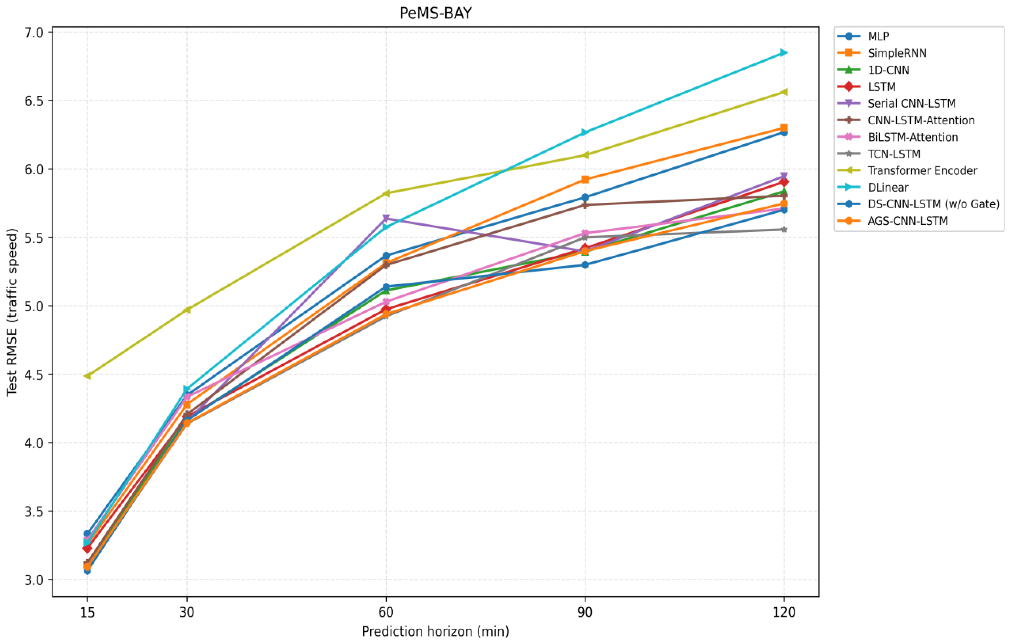
	AGS-CNN-LSTM	5.747	3.246	6.058	0.4166

presents the prediction results of each model on the PeMS-BAY test set, and Figure 4 visualizes the variation trend of test-set RMSE with the prediction horizon for different models on this dataset.

As shown in Table 7, in the single-sensor traffic speed prediction task on PeMS-BAY, different models exhibit varying performance across different prediction horizons. TCN-LSTM achieves lower RMSE and higher ${\mathrm{R}}^2$ on the 30 min, 60 min, and 120 min tasks, indicating that the combination of dilated causal convolution and LSTM has strong temporal pattern modeling capability for univariate speed sequences. DS-CNN-LSTM (w/o Gate) achieves the best RMSE and ${\mathrm{R}}^2$ on the 15 min and 90 min tasks, suggesting that the parallel dual-stream late-fusion structure itself can effectively extract local variation features and temporal dependency features.

In comparison, AGS-CNN-LSTM does not achieve the best results across all prediction horizons on PeMS-BAY, but it shows strong competitiveness on the 30 min and 60 min tasks. Specifically, AGS-CNN-LSTM obtains an RMSE of 4.142 on the 30 min task, only slightly higher than the best value of 4.138 achieved by TCN-LSTM. On the 60 min task, its RMSE is 4.938, which is also close to the best value of 4.922 achieved by TCN-LSTM. Meanwhile, AGS-CNN-LSTM achieves the best MAE on both the 30 min and 60 min tasks, indicating that it can effectively reduce the average absolute error in some short- and medium-term prediction scenarios.

From the performance of different types of baseline models, Transformer Encoder does not show a clear advantage under the current historical window length of K = 12, suggesting that when the input historical window is relatively short, the advantage of the global self-attention mechanism may not be fully realized. DLinear shows relatively high overall errors on this dataset, indicating that relying only on linear trend decomposition is insufficient to fully characterize nonlinear fluctuations in single-sensor traffic speed sequences. Overall, the PeMS-BAY experimental results indicate that AGS-CNN-LSTM is competitive in some short- and medium-term prediction tasks, but its performance advantage does not remain stable across all prediction horizons.

4.2. Analysis of Traffic Flow Prediction Results on the PeMSD8 Dataset

Under the experimental setting of this paper, the PeMSD8 dataset corresponds to a multi-node single-channel traffic flow prediction task. This experiment is used to examine the prediction capability of different models under multi-node traffic-state sequence inputs.

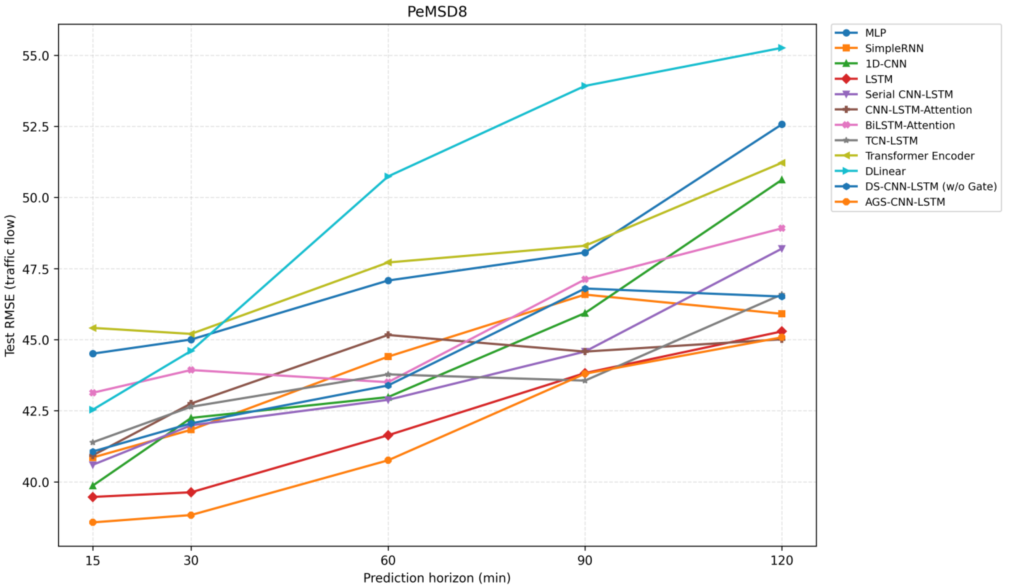
As shown in

Table 8. Evaluation results on the PeMSD8 test set.

Horizon	Model	RMSE	MAE	MAPE	${\mathit{R}}^2$
15 min	MLP	44.505	28.694	17.732	0.9089
	SimpleRNN	40.853	26.022	15.697	0.9232
	1D-CNN	39.863	25.061	14.729	0.9269
	LSTM	39.468	24.466	14.711	0.9283
	Serial CNN-LSTM	40.596	24.761	14.656	0.9242
	CNN-LSTM-Attention	40.927	25.354	15.382	0.9229
	BiLSTM-Attention	43.129	27.522	16.415	0.9144
	TCN-LSTM	41.388	25.346	14.992	0.9212
	Transformer Encoder	45.411	29.610	18.158	0.9051
	DLinear	42.533	29.420	17.416	0.9168
	DS-CNN-LSTM (w/o Gate)	41.064	25.295	15.324	0.9224
	AGS-CNN-LSTM	38.572	24.216	14.415	0.9315
30 min	MLP	45.003	29.146	17.785	0.9068
	SimpleRNN	41.829	27.092	16.390	0.9195
	1D-CNN	42.246	26.547	15.551	0.9179
	LSTM	39.630	24.651	14.765	0.9278
	Serial CNN-LSTM	41.986	26.638	15.908	0.9189
	CNN-LSTM-Attention	42.753	27.408	16.499	0.9159
	BiLSTM-Attention	43.930	28.310	17.312	0.9112
	TCN-LSTM	42.638	26.817	16.043	0.9164
	Transformer Encoder	45.200	29.577	18.010	0.9060
	DLinear	44.603	30.403	18.222	0.9085
	DS-CNN-LSTM (w/o Gate)	42.054	26.395	15.551	0.9187
	AGS-CNN-LSTM	38.831	24.680	14.809	0.9306
60 min	MLP	47.076	30.666	18.813	0.8981
	SimpleRNN	44.399	29.093	17.285	0.9094
	1D-CNN	42.977	27.530	16.219	0.9151
	LSTM	41.636	26.266	15.365	0.9203
	Serial CNN-LSTM	42.880	27.330	15.952	0.9155
	CNN-LSTM-Attention	45.162	29.767	17.405	0.9062
	BiLSTM-Attention	43.501	28.482	16.823	0.9130
	TCN-LSTM	43.777	27.859	16.565	0.9119
	Transformer Encoder	47.711	31.985	19.288	0.8953
	DLinear	50.736	34.886	20.617	0.8816
	DS-CNN-LSTM (w/o Gate)	43.387	27.527	16.665	0.9134
	AGS-CNN-LSTM	40.754	25.801	15.251	0.9236
90 min	MLP	48.063	31.683	19.148	0.8938
	SimpleRNN	46.582	30.894	18.675	0.9003
	1D-CNN	45.932	30.157	17.116	0.9030
	LSTM	43.822	28.138	16.056	0.9117
	Serial CNN-LSTM	44.578	28.273	16.530	0.9087
	CNN-LSTM-Attention	44.577	28.275	16.285	0.9087
	BiLSTM-Attention	47.115	31.300	17.732	0.8980
	TCN-LSTM	43.557	27.765	16.283	0.9128
	Transformer Encoder	48.299	32.883	20.102	0.8928
	DLinear	53.920	36.229	21.325	0.8664
	DS-CNN-LSTM (w/o Gate)	46.796	30.689	17.890	0.8993
	AGS-CNN-LSTM	43.799	28.041	15.995	0.9118
120 min	MLP	52.568	34.631	19.996	0.8730
	SimpleRNN	45.906	30.597	18.911	0.9032
	1D-CNN	50.618	34.518	18.818	0.8823
	LSTM	45.287	29.379	16.180	0.9058
	Serial CNN-LSTM	48.198	32.220	17.799	0.8933
	CNN-LSTM-Attention	45.010	28.892	16.606	0.9069
	BiLSTM-Attention	48.911	32.463	17.959	0.8901
	TCN-LSTM	46.587	30.510	17.145	0.9003
	Transformer Encoder	51.217	34.330	19.884	0.8795
	DLinear	55.258	38.005	22.195	0.8597
	DS-CNN-LSTM (w/o Gate)	46.513	30.902	17.600	0.9006
	AGS-CNN-LSTM	45.080	29.202	16.459	0.9066

Note: Bold values indicate the best performance under the corresponding prediction horizon or experimental setting.

, in the PeMSD8 multi-node traffic flow prediction task, AGS-CNN-LSTM shows relatively stable overall performance. Specifically, AGS-CNN-LSTM achieves the lowest RMSE and the highest ${\mathrm{R}}^2$ on the 15 min, 30 min, and 60 min tasks, indicating that the proposed structure has good overall error-control capability and trend-fitting capability in short- to medium-term multi-node traffic flow prediction.

On the 90 min and 120 min tasks, although AGS-CNN-LSTM does not achieve the lowest RMSE, it still maintains only a small gap from the best-performing model. For the 90 min task, TCN-LSTM obtains the lowest RMSE of 43.557, while AGS-CNN-LSTM obtains an RMSE of 43.799, with only a small difference between them. For the 120 min task, CNN-LSTM-Attention achieves the lowest RMSE of 45.010, while AGS-CNN-LSTM obtains an RMSE of 45.080, again showing only a small gap. These results indicate that attention-enhanced models and temporal convolutional structures remain highly competitive over longer prediction horizons, while AGS-CNN-LSTM can still maintain near-optimal prediction performance.

From the perspective of different model types, Transformer Encoder does not show a stable advantage on PeMSD8, which may be related to the relatively short historical window length adopted in this paper. DLinear exhibits relatively higher errors under longer prediction horizons, indicating that the linear decomposition structure has relatively limited capability in characterizing nonlinear fluctuations in complex multi-node traffic flow changes. In contrast, AGS-CNN-LSTM extracts local variation features and temporal dependency features in parallel, and introduces a recent-state anchor through the adaptive gated shortcut, thereby showing good adaptability in the multi-node traffic flow prediction task. Figure 5 further illustrates the variation trend of test-set RMSE with the prediction horizon for different models on the PeMSD8 dataset.

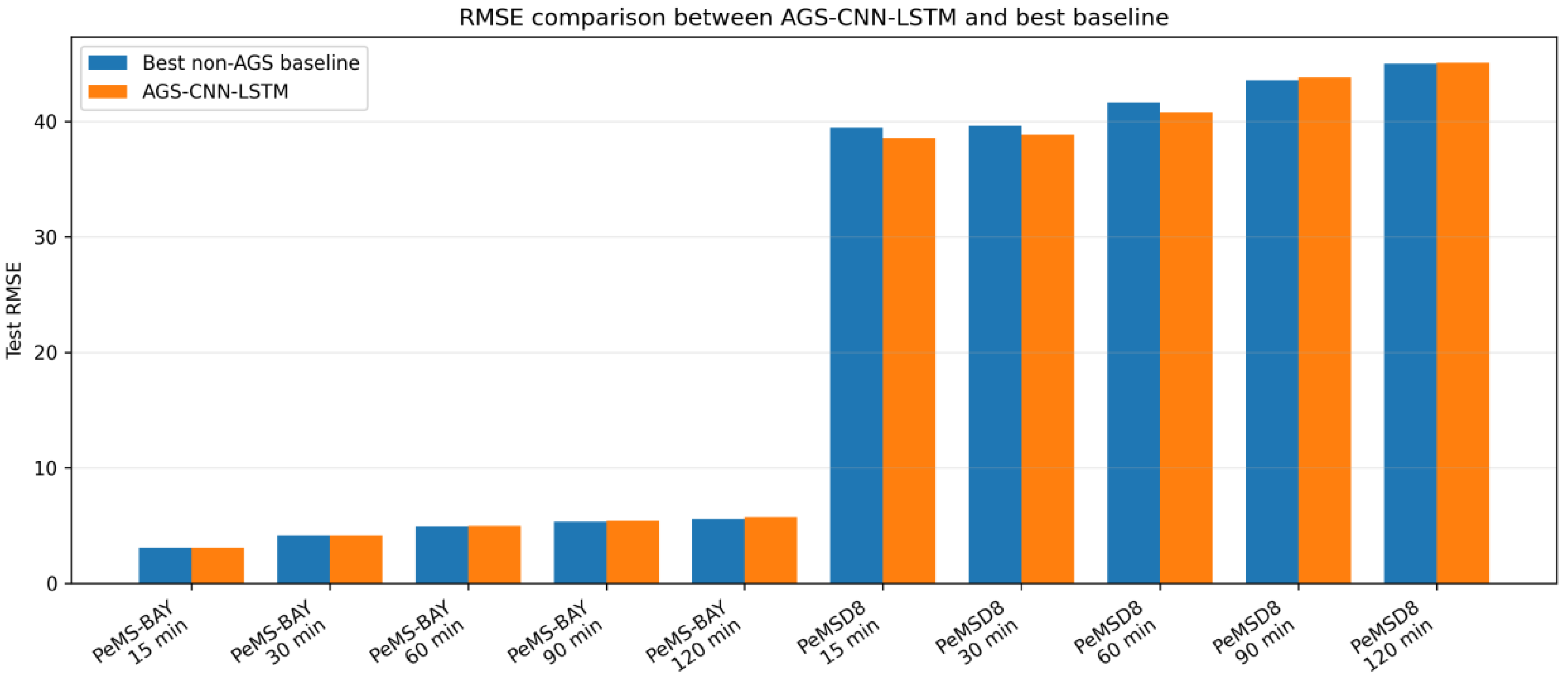
To intuitively compare the difference between AGS-CNN-LSTM and the best baseline model under each prediction horizon, this paper selects the non-AGS model with the lowest RMSE at each prediction horizon as the best baseline and compares it with AGS-CNN-LSTM. The results are shown in Figure 6. Since the best baseline model may vary across different datasets and prediction horizons, Figure 6 is mainly used to illustrate the error gap between AGS-CNN-LSTM and the current best non-AGS model under different prediction horizons.

As shown in Figure 6, on the PeMS-BAY dataset, AGS-CNN-LSTM does not achieve the lowest RMSE across all prediction horizons. Specifically, DS-CNN-LSTM (w/o Gate) serves as the best baseline on the 15 min and 90 min tasks, while TCN-LSTM serves as the best baseline on the 30 min, 60 min, and 120 min tasks. AGS-CNN-LSTM is very close to the best baseline on the 30 min and 60 min tasks, but the gap becomes larger on the 90 min and 120 min tasks, indicating that its advantage in the single-sensor speed prediction task is dependent on the prediction horizon.

For the PeMSD8 dataset, AGS-CNN-LSTM outperforms all non-AGS baselines on the 15 min, 30 min, and 60 min tasks. On the 90 min and 120 min tasks, although TCN-LSTM and CNN-LSTM-Attention achieve the lowest RMSE, respectively, the gap between AGS-CNN-LSTM and the best baseline remains small. This result indicates that, in the multi-node traffic flow prediction scenario, the proposed dual-stream late-fusion structure and adaptive gated shortcut can provide relatively stable performance.

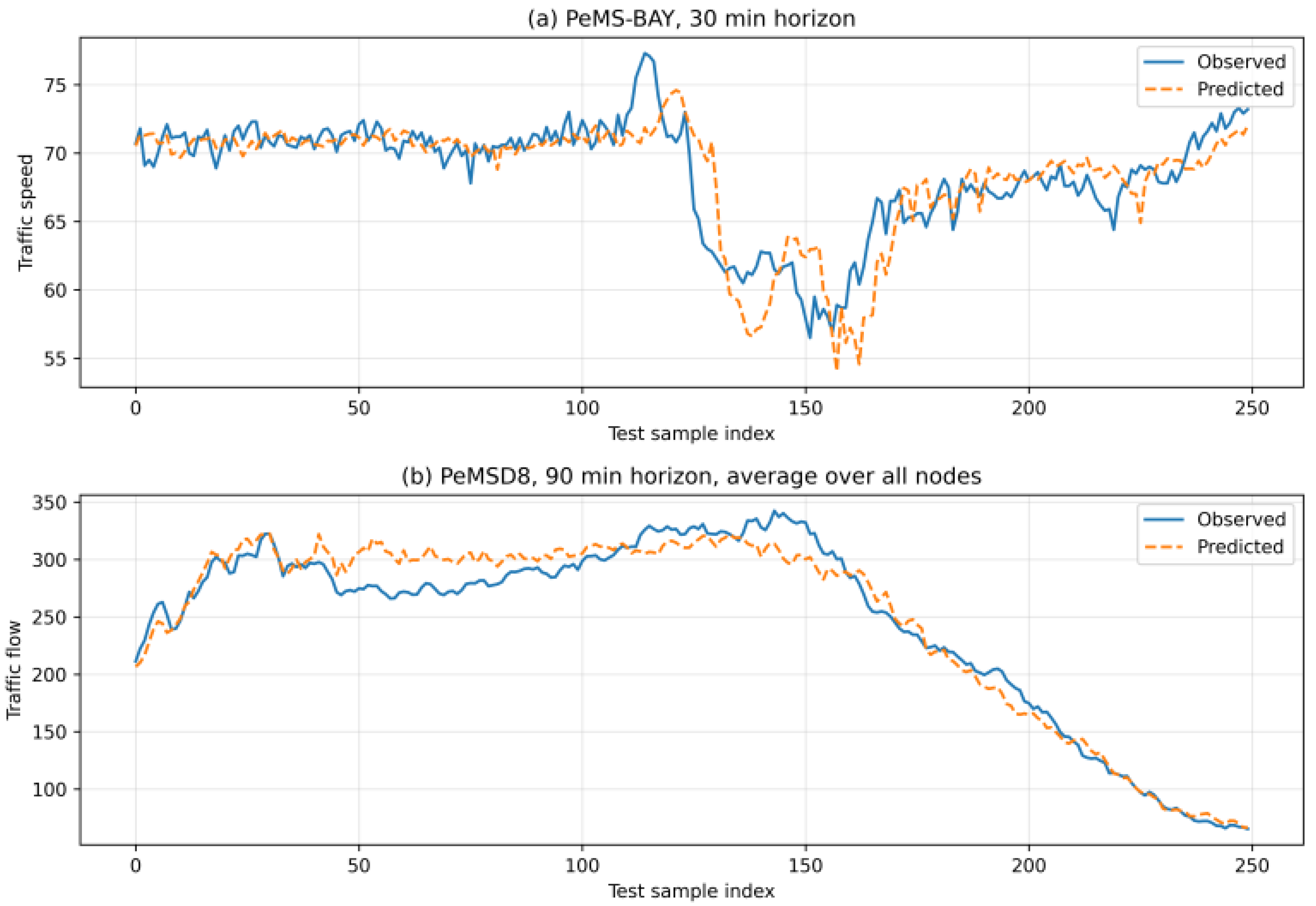
In addition to error metrics and model comparisons, this paper selects representative prediction tasks to visualize the predicted values and true observations of AGS-CNN-LSTM, so as to more intuitively demonstrate the model’s ability to track actual traffic-state variations. Figure 7 analyzes two tasks: PeMS-BAY 30 min and PeMSD8 90 min. The PeMS-BAY 30 min task corresponds to the case where AGS-CNN-LSTM performs close to the best baseline in single-sensor traffic speed prediction, while the PeMSD8 90 min task corresponds to a longer-horizon prediction task where AGS-CNN-LSTM maintains only a small gap from the best model in multi-node traffic flow prediction. For PeMSD8, since the dataset corresponds to a multi-node single-channel traffic flow prediction task, Figure 7b presents the average true flow and average predicted flow over all monitoring sensors for each test sample.

As shown in Figure 7, AGS-CNN-LSTM can follow the overall variation trend of the true traffic states for most test samples, indicating that the dual-stream late-fusion structure can effectively capture the main evolutionary patterns of traffic sequences. At the same time, during periods with local abrupt changes or large fluctuation amplitudes, the prediction curves still show certain lagging and smoothing effects. This indicates that, when only historical traffic-state sequences are used, the model’s ability to characterize sudden disturbances remains limited. This phenomenon is generally consistent with the results in Table 7 and Table 8, where the errors vary as the prediction horizon extends, and further suggests that the proposed model still has room for improvement in complex fluctuation scenarios and longer prediction horizons.

4.3. Ablation Experiments and Analysis of the Gated Shortcut Mechanism

To more clearly analyze the roles of different structural designs in AGS-CNN-LSTM, this paper treats Serial CNN-LSTM, DS-CNN-LSTM (w/o Gate), and AGS-CNN-LSTM as a group of progressively enhanced structures for comparison. Among them, Serial CNN-LSTM represents the conventional serial CNN-LSTM structure; DS-CNN-LSTM (w/o Gate) represents a structure that adopts parallel dual-stream late fusion but does not introduce the recent-state anchor or the adaptive gated shortcut; and AGS-CNN-LSTM further incorporates the adaptive gated shortcut based on the parallel dual-stream late-fusion structure. By comparing the performance of these three models under different prediction horizons, the effects of the serial/parallel structure, late fusion, and gated recent-state supplementation mechanism can be analyzed separately.

To analyze the actual role of the adaptive gated shortcut, this paper compares the complete AGS-CNN-LSTM with DS-CNN-LSTM (w/o Gate), from which the gated shortcut is removed. Both models adopt the same parallel CNN branch, LSTM branch, and late-fusion structure. The difference is that AGS-CNN-LSTM introduces the observation at the end of the input sequence as a recent-state anchor and generates dynamic gate weights from the deep fused features.

Table 9. Ablation experiment results of the adaptive gated shortcut.

Dataset	Horizon	Model	RMSE	MAE	MAPE	${\mathit{R}}^2$
PeMS-BAY	15 min	DS-CNN-LSTM (w/o Gate)	3.064	1.540	2.778	0.8341
		AGS-CNN-LSTM	3.094	1.592	2.861	0.8309
	30 min	DS-CNN-LSTM (w/o Gate)	4.162	2.055	3.890	0.6940
		AGS-CNN-LSTM	4.142	2.017	3.841	0.6970
	60 min	DS-CNN-LSTM (w/o Gate)	5.139	2.768	5.283	0.5335
		AGS-CNN-LSTM	4.938	2.453	4.834	0.5692
	90 min	DS-CNN-LSTM (w/o Gate)	5.298	2.701	5.295	0.5043
		AGS-CNN-LSTM	5.399	2.820	5.476	0.4851
	120 min	DS-CNN-LSTM (w/o Gate)	5.701	3.068	5.852	0.4260
		AGS-CNN-LSTM	5.747	3.246	6.058	0.4166
PeMSD8	15 min	DS-CNN-LSTM (w/o Gate)	41.064	25.295	15.324	0.9224
		AGS-CNN-LSTM	38.572	24.216	14.415	0.9315
	30 min	DS-CNN-LSTM (w/o Gate)	42.054	26.395	15.551	0.9187
		AGS-CNN-LSTM	38.831	24.680	14.809	0.9306
	60 min	DS-CNN-LSTM (w/o Gate)	43.387	27.527	16.665	0.9134
		AGS-CNN-LSTM	40.754	25.801	15.251	0.9236
	90 min	DS-CNN-LSTM (w/o Gate)	46.796	30.689	17.890	0.8993
		AGS-CNN-LSTM	43.799	28.041	15.995	0.9118
	120 min	DS-CNN-LSTM (w/o Gate)	46.513	30.902	17.600	0.9006
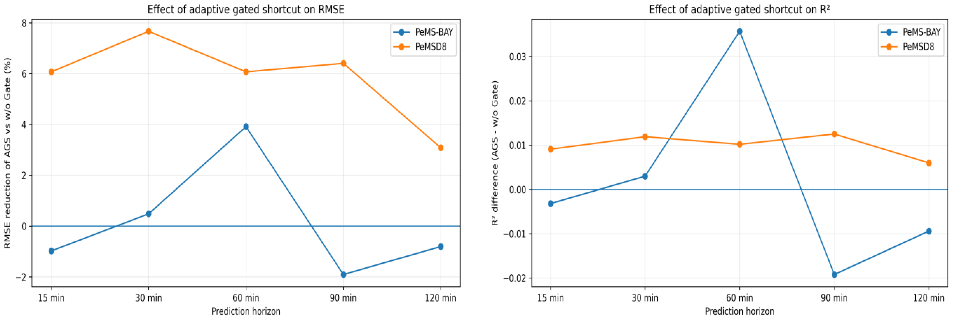
		AGS-CNN-LSTM	45.080	29.202	16.459	0.9066

presents the ablation experiment results.

As shown in Table 9, the adaptive gated shortcut does not consistently lead to improvement in all scenarios, but instead shows clear dataset differences and prediction-horizon dependence. On the PeMSD8 dataset, AGS-CNN-LSTM achieves lower RMSE than DS-CNN-LSTM (w/o Gate) across all five prediction horizons, with reductions of approximately 3.08–7.66%. Meanwhile, AGS-CNN-LSTM also achieves higher ${\mathrm{R}}^2$ across all five prediction horizons, indicating that, in the multi-node traffic flow prediction task, the recent-state anchor at the end of the input sequence can provide a relatively stable supplement to the deep dual-stream fused features. In contrast, on the PeMS-BAY dataset, the benefit of the gated shortcut is more dependent on the prediction horizon. AGS-CNN-LSTM achieves lower RMSE than DS-CNN-LSTM (w/o Gate) on the 30 min and 60 min tasks, with the RMSE reduction reaching 3.91% on the 60 min task. However, on the 15 min, 90 min, and 120 min tasks, DS-CNN-LSTM (w/o Gate), after removing the gated shortcut, performs better instead. This suggests that, for a single-sensor traffic speed sequence, introducing the recent-state anchor does not necessarily bring stable gains, and its effectiveness depends on the correlation between the state at the end of the input sequence and the future prediction target.

Combined with Table 9 and Figure 8, it can be further observed that the contribution of the gated shortcut is more stable on PeMSD8, whereas it shows greater uncertainty on PeMS-BAY. This phenomenon may be related to the different input organization forms of the two datasets. PeMSD8 corresponds to a multi-node traffic flow prediction task, in which the input contains synchronous traffic-state variations from multiple monitoring sensors. Therefore, the state at the end of the input sequence has relatively strong reference value for future overall flow changes. In contrast, PeMS-BAY is treated as a single-sensor speed prediction task in this paper, where the local speed sequence may be more strongly affected by short-term disturbances. As a result, the recent-state anchor may introduce short-term bias under longer prediction horizons.

This result indicates that the adaptive gated shortcut designed in this paper is more suitable as a recent-state supplementation mechanism, rather than as a universal enhancement module applicable to all prediction scenarios. Conventional residual connections usually transmit intermediate hidden features, whereas the shortcut branch in this paper transmits the raw observed state at the end of the input sequence. Conventional gated fusion is often used to regulate the weights among different hidden-feature branches, whereas the gate weights in this paper are generated from the deep dual-stream fused features and are used to regulate the contribution of the recent-state anchor to the final prediction. Therefore, the main function of the adaptive gated shortcut is to dynamically coordinate deep historical representations and recent raw-state information. This also indicates that the practical value of the gated shortcut lies in providing a low-cost recent-state supplementation path, rather than guaranteeing performance improvement under all traffic conditions or all prediction horizons.

It should be pointed out that the ablation experiment results do not support interpreting the adaptive gated shortcut as a universal enhancement module that can consistently improve performance in all scenarios. Instead, its effect shows clear dependence on the dataset and prediction horizon. When the observation at the end of the input sequence remains strongly correlated with the future prediction target, the recent-state anchor can provide an effective supplement to the deep fused features. However, when the prediction horizon is longer or traffic-state fluctuations are more complex, recent-state information may no longer provide stable reference value and may even introduce short-term state bias. Therefore, the practical necessity of the adaptive gated shortcut mainly lies in its ability to provide the model with a learnable recent-state regulation channel, rather than in guaranteeing performance improvement across all tasks. Combined with the model complexity analysis, this mechanism introduces only a very small number of additional parameters on PeMS-BAY. Although it increases the number of parameters to some extent on PeMSD8, its training and inference times remain at the same order of magnitude as those of the ungated dual-stream structure. Therefore, this paper positions the proposed mechanism as a conditional fusion improvement with low additional computational cost, rather than as a complex structure that is universally superior to all baselines.

4.4. Difference Analysis with Typical Baseline Models

From the above experimental results, it can be seen that different types of baseline models show clear performance differences across the two datasets and different prediction horizons. Serial CNN-LSTM remains competitive in some tasks, indicating that the serial convolutional–recurrent structure can effectively extract local variations and temporal dependency information. However, its feature transmission path is relatively fixed, making it difficult to explicitly distinguish the roles of local variation features and temporal dependency features. DS-CNN-LSTM (w/o Gate) alleviates this problem through parallel branches and late fusion, and achieves favorable results under some prediction horizons on PeMS-BAY, suggesting that the parallel dual-stream late-fusion structure itself is already effective to some extent.

Compared with attention-enhanced models and TCN-LSTM, the difference of AGS-CNN-LSTM does not lie in enhancing global temporal weight allocation or expanding the convolutional receptive field. Instead, it introduces the raw observation at the end of the input sequence as a recent-state anchor and dynamically regulates its contribution through deep fused features. The experimental results show that this mechanism performs more stably in the PeMSD8 multi-node traffic flow prediction task, while in the PeMS-BAY single-sensor speed prediction task, it mainly maintains performance close to strong temporal baselines. This indicates that its effectiveness is influenced by the dataset structure and prediction horizon.

Therefore, AGS-CNN-LSTM is more appropriately positioned as a lightweight fusion-mechanism improvement method under settings without explicit topology input. Its value mainly lies in providing a recent-state-supplemented information-flow organization strategy for CNN-LSTM-based models, rather than serving as a comprehensive replacement for complex spatiotemporal prediction models.

4.5. Sensitivity Analysis

To further analyze the influence of key parameter changes on the prediction performance of AGS-CNN-LSTM, this paper selects the historical observation window length K and the number of LSTM hidden units as the objects of sensitivity analysis, with test-set RMSE used as the main evaluation metric. The historical observation window length K determines the range of historical traffic states that the model can use, while the number of LSTM hidden units affects the representation capability of temporal dependency features. By analyzing the effects of these parameters across different datasets and prediction horizons, the performance stability and applicability boundaries of the proposed model under different settings can be further examined.

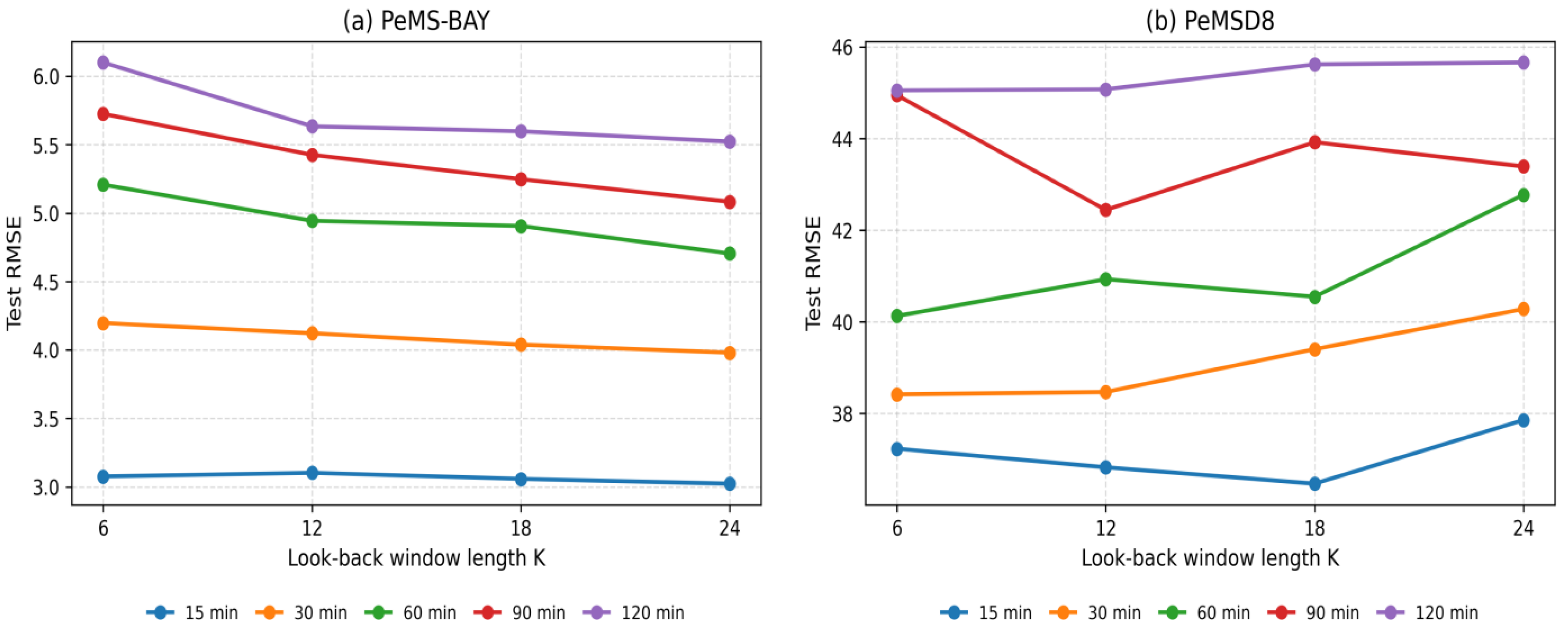
In the sensitivity analysis of historical window length, this paper sets K = 6, 12, 18, and 24, while fixing the number of LSTM hidden units at 64 and the number of CNN filters at 64. In the sensitivity analysis of LSTM hidden units, the number of hidden units is set to 16, 32, 64, 128, while the historical window length is fixed at K = 12 and the number of CNN filters is fixed at 64. Both groups of sensitivity analyses cover five prediction horizons: 15 min, 30 min, 60 min, 90 min, and 120 min.

As shown in

Table 10. Effect of historical observation window length K on the test-set RMSE of AGS-CNN-LSTM.

Dataset	K	15 min	30 min	60 min	90 min	120 min
PeMS-BAY	6	3.076	4.197	5.208	5.725	6.101
	12	3.102	4.122	4.944	5.426	5.635
	18	3.058	4.039	4.906	5.248	5.598
	24	3.023	3.980	4.705	5.083	5.523
PeMSD8	6	37.231	38.418	40.130	44.948	45.055
	12	36.825	38.469	40.931	42.444	45.076
	18	36.468	39.403	40.549	43.923	45.620
	24	37.856	40.280	42.775	43.392	45.663

Note: Bold values indicate the best performance under the corresponding prediction horizon or experimental setting.

and Figure 9, the historical window length has different effects on the two datasets. On the PeMS-BAY dataset, as K increases from 6 to 24, the RMSE generally decreases across the five prediction horizons, indicating that the single-sensor traffic speed sequence can benefit to some extent from a longer historical context. Especially for the 60 min, 90 min, and 120 min tasks, a longer historical window can clearly reduce prediction errors, suggesting that medium- and long-term speed prediction is more sensitive to historical speed variation information.

Different from PeMS-BAY, the performance under different historical window lengths on the PeMSD8 dataset does not show a monotonic trend. K = 6, K = 12, and K = 18 achieve relatively lower RMSE under different prediction horizons, whereas K = 24 does not consistently lead to better results. This indicates that, in the multi-node traffic flow prediction task, an excessively long historical window may introduce more fluctuation information and is not necessarily beneficial for model prediction. In contrast, a short or moderate historical window can achieve a better balance between retaining recent traffic-state information and controlling input complexity.

As shown in

Table 11. Effect of the number of LSTM hidden units on the test-set RMSE of AGS-CNN-LSTM.

Dataset	Hidden Units	15 min	30 min	60 min	90 min	120 min
PeMS-BAY	16	3.062	4.097	4.920	5.337	5.647
	32	3.063	4.143	4.973	5.545	5.708
	64	3.102	4.122	4.944	5.426	5.635
	128	3.070	4.163	4.958	5.412	5.613
PeMSD8	16	36.193	38.322	40.984	43.587	44.716
	32	37.336	38.596	41.624	43.740	44.828
	64	36.825	38.469	40.931	42.444	45.076
	128	37.694	39.147	41.057	43.385	44.680

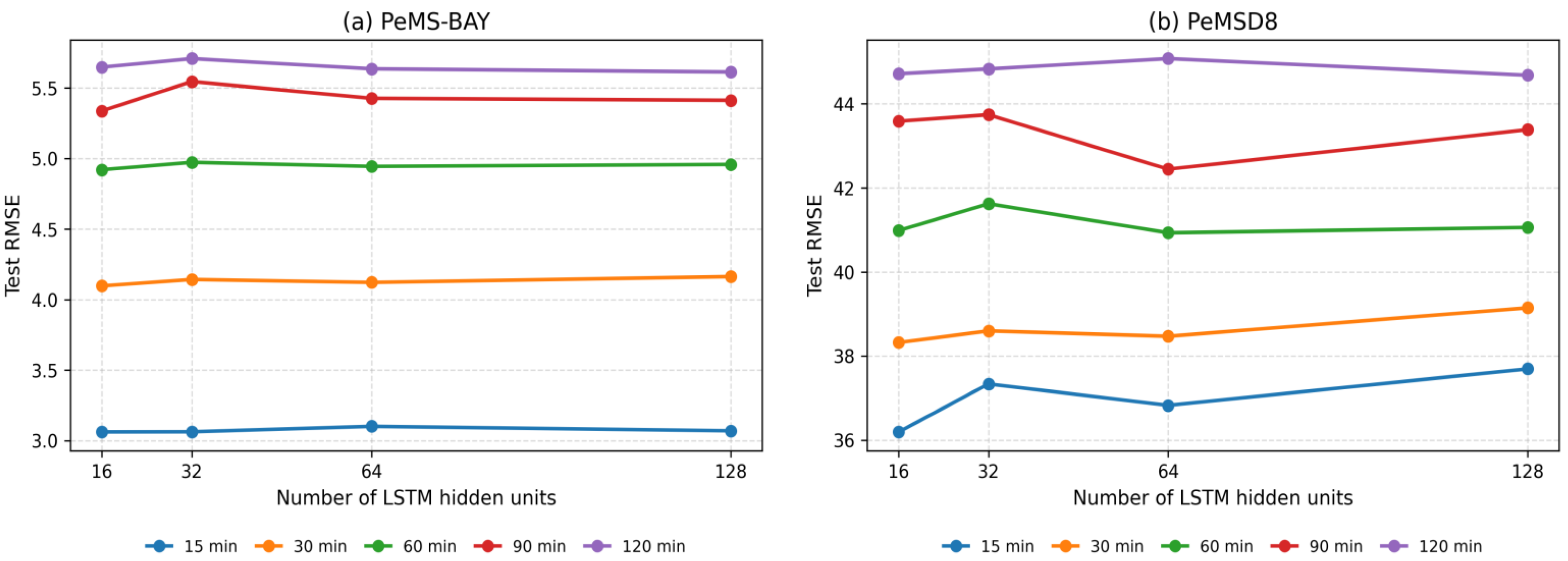
Note: Bold values indicate the best performance under the corresponding prediction horizon or experimental setting.

and Figure 10, increasing the number of LSTM hidden units does not lead to monotonic performance improvement on either dataset. On the PeMS-BAY dataset, hidden units = 16 achieves lower RMSE on the 15 min, 30 min, 60 min, and 90 min tasks, while hidden units = 128 is only slightly better on the 120 min task. This indicates that, for the single-sensor traffic speed sequence, a relatively small LSTM hidden size is already sufficient to characterize the main temporal dependencies, and an excessively large hidden dimension does not necessarily improve prediction performance.

On the PeMSD8 dataset, different numbers of hidden units also show varying performance across different prediction horizons. Hidden units = 16 performs better on the 15 min and 30 min tasks, hidden units = 64 achieves lower RMSE on the 60 min and 90 min tasks, while hidden units = 128 is only slightly better on the 120 min task. This result suggests that multi-node traffic flow prediction requires a certain degree of temporal feature representation capability, but simply increasing the number of LSTM hidden units cannot consistently reduce prediction errors.

Overall, the performance of AGS-CNN-LSTM is affected by both the historical window length and the number of LSTM hidden units, but the variation patterns show clear dependence on the dataset and prediction horizon. PeMS-BAY is more sensitive to the historical window length, and a longer historical window helps reduce the prediction error of single-sensor speed forecasting. PeMSD8 shows more complex responses to both window length and hidden-unit number, indicating that model performance in multi-node traffic flow prediction is jointly influenced by factors such as synchronous variations among nodes, local fluctuations, and input complexity. The main experiments in this paper adopt K = 12 and LSTM hidden units = 64 as the unified settings, mainly to ensure consistent comparisons across different models, datasets, and prediction horizons. The sensitivity analysis results indicate that further tuning key parameters for specific datasets and prediction tasks may bring additional performance improvements, but the overall performance of the proposed model does not completely depend on a single parameter setting.

4.6. Multi-Seed Stability and Significance Analysis

To reduce the influence of random initialization on the experimental results and further examine the stability of model performance differences, this paper selects several representative models, including LSTM, Serial CNN-LSTM, CNN-LSTM-Attention, TCN-LSTM, DS-CNN-LSTM (w/o Gate), and AGS-CNN-LSTM, and repeats the experiments under three random seeds, namely 42, 2024, and 3407. The experiments cover the PeMS-BAY and PeMSD8 datasets, as well as five prediction horizons: 15 min, 30 min, 60 min, 90 min, and 120 min.

This paper uses the mean ± standard deviation of RMSE to describe model stability under different random initialization conditions. In addition, AGS-CNN-LSTM is further compared with the best non-AGS baseline model under the corresponding prediction horizon. The results are shown in

Table 12. Multi-seed comparison results between AGS-CNN-LSTM and the best non-AGS baseline.

Dataset	Horizon	Best Non-AGS Baseline	AGS-CNN-LSTM RMSE	Baseline RMSE	ΔRMSE	Relative Δ/%
PeMS-BAY	15 min	DS-CNN-LSTM (w/o Gate)	$3.087\pm 0.017$	$3.091\pm 0.029$	−0.004	−0.14
	30 min	TCN-LSTM	$4.149\pm 0.046$	$4.131\pm 0.035$	0.018	0.44
	60 min	TCN-LSTM	$5.028\pm 0.097$	$4.969\pm 0.100$	0.060	1.20
	90 min	TCN-LSTM	$5.406\pm 0.046$	$5.280\pm 0.084$	0.126	2.38
	120 min	TCN-LSTM	$5.654\pm 0.051$	$5.658\pm 0.151$	−0.005	−0.08
PeMSD8	15 min	LSTM	$36.997\pm 0.154$	$39.001\pm 0.344$	−2.004	−5.14
	30 min	LSTM	$38.643\pm 0.293$	$40.122\pm 0.398$	−1.479	−3.69
	60 min	LSTM	$41.279\pm 0.553$	$41.947\pm 0.388$	−0.668	−1.59
	90 min	LSTM	$43.448\pm 1.125$	$44.220\pm 0.462$	−0.772	−1.75
	120 min	LSTM	$44.167\pm 0.825$	$45.478\pm 0.592$	−1.311	−2.88

.

As shown in Table 12, in the PeMS-BAY single-sensor speed prediction task, AGS-CNN-LSTM remains generally close to the best non-AGS baseline model, but its advantage is not stable. Specifically, AGS-CNN-LSTM achieves slightly lower average RMSE on the 15 min and 120 min tasks, but the relative differences are only −0.14% and −0.08%, respectively. On the 30 min, 60 min, and 90 min tasks, TCN-LSTM achieves lower average RMSE. This result indicates that, in the single-sensor speed sequence prediction task, the benefit brought by the adaptive gated shortcut is clearly dependent on the prediction horizon, and the model does not outperform strong temporal baselines across all prediction horizons.

In contrast, in the PeMSD8 multi-node traffic flow prediction task, AGS-CNN-LSTM achieves lower average RMSE than the best non-AGS baseline across all five prediction horizons. Compared with the corresponding best non-AGS baseline, AGS-CNN-LSTM reduces RMSE by 1.59–5.14%, with more obvious improvements on the 15 min and 30 min tasks. This suggests that, in multi-node traffic flow prediction scenarios, the recent-state anchor and adaptive gated regulation mechanism can provide a more stable performance supplement to the dual-stream late-fusion structure.

To further analyze the performance differences, this paper conducts paired significance tests. It should be noted that, since the multi-seed experiments use only three random seeds, the sample size for seed-level significance testing is small; therefore, the results are used only as auxiliary evidence. The experimental results show that, on the PeMSD8 dataset, the seed-level paired t-test between AGS-CNN-LSTM and the best non-AGS baseline reaches the 0.05 significance level on the 15 min, 30 min, 60 min, and 120 min tasks, while the 90 min task does not reach the significance level. On the PeMS-BAY dataset, the seed-level differences between AGS-CNN-LSTM and the best non-AGS baseline do not reach the 0.05 significance level. Overall, the multi-seed experiments further indicate that AGS-CNN-LSTM has a more stable advantage in the PeMSD8 multi-node flow prediction task, whereas in the PeMS-BAY single-sensor speed prediction task, it mainly performs close to strong baseline models, and its benefit is strongly influenced by dataset characteristics and prediction horizon. It should also be emphasized that “competitive performance” in this paper does not mean consistent superiority over all comparison models. Instead, it means that AGS-CNN-LSTM can achieve performance close to or better than strong non-graph baselines in several constrained prediction settings while maintaining a simple input structure and controllable computational cost. Therefore, the metric gains reported in this study should be interpreted cautiously as scenario-dependent improvements, rather than as evidence of universal practical dominance.

4.7. Robustness Analysis Under Noise Perturbations

To further analyze the robustness of the model under input perturbations, this paper adds Gaussian noise with different intensities to the test input sequences to simulate possible measurement disturbances in real traffic sensors. Specifically, the training process still uses the original training set, without adding extra noise to the training data. During the testing stage, noise perturbations are added to the normalized test input $X_{\mathrm{test}}$, and the perturbed inputs are clipped to the interval [0,1]. The noisy input can be expressed as follows:

$$X_{\mathrm{noise}}=clip\left(X_{\mathrm{test}}+\alpha ·std\left(X_{\mathrm{train}}\right)·ϵ,0,1\right)$$

where $ϵ$ denotes random noise following a standard normal distribution, and $\alpha$ denotes the noise intensity. In this paper, $\alpha$ is set to 0.05, 0.10, and 0.15. Three models, namely TCN-LSTM, DS-CNN-LSTM (w/o Gate), and AGS-CNN-LSTM, are selected for comparison under the 30 min, 60 min, and 120 min prediction tasks. For each noise level, three noise random seeds, namely 42, 2024, and 3407, are used to repeatedly generate perturbed inputs, and the RMSE increase rate relative to the clean test input is reported. It should be noted that this experiment aims to evaluate the sensitivity of the models to general input noise perturbations and is not equivalent to a complete sensor fault repair or missing-data recovery task.

The RMSE increase rate is defined as follows:

$$RMS{E}_{increase}={\displaystyle \frac{RMS{E}_{noise}-RMS{E}_{clean}}{RMS{E}_{clean}}}\times 100\%$$

As shown in

Table 13. Comparison of RMSE increase rates under different noise levels.

Dataset	Horizon	Model	5% Noise	10% Noise	15% Noise
PeMS-BAY	30 min	AGS-CNN-LSTM	0.329	1.400	3.404
		DS-CNN-LSTM (w/o Gate)	0.456	2.145	5.466
		TCN-LSTM	0.360	1.499	3.679
PeMS-BAY	60 min	AGS-CNN-LSTM	0.377	1.681	4.627
		DS-CNN-LSTM (w/o Gate)	0.322	1.484	3.929
		TCN-LSTM	0.416	1.991	5.808
PeMS-BAY	120 min	AGS-CNN-LSTM	0.582	3.021	8.830
		DS-CNN-LSTM (w/o Gate)	0.706	3.412	9.859
		TCN-LSTM	0.698	3.486	11.610
PeMSD8	30 min	AGS-CNN-LSTM	0.176	0.729	1.650
		DS-CNN-LSTM (w/o Gate)	0.071	0.265	0.592
		TCN-LSTM	0.029	0.102	0.222
PeMSD8	60 min	AGS-CNN-LSTM	0.178	0.648	1.419
		DS-CNN-LSTM (w/o Gate)	0.112	0.371	0.793
		TCN-LSTM	0.118	0.354	0.721
PeMSD8	120 min	AGS-CNN-LSTM	0.226	0.728	1.598
		DS-CNN-LSTM (w/o Gate)	0.346	1.054	2.194
		TCN-LSTM	0.270	0.778	1.510

, as the noise level increases from 5% to 15%, the RMSE increase rates of all models generally rise, indicating that input perturbations weaken prediction performance. On the PeMS-BAY dataset, AGS-CNN-LSTM shows lower RMSE increase rates on the 30 min and 120 min tasks, whereas DS-CNN-LSTM (w/o Gate) is more stable on the 60 min task. On the PeMSD8 dataset, AGS-CNN-LSTM is mainly competitive on the 120 min task, while TCN-LSTM or DS-CNN-LSTM (w/o Gate) exhibits lower noise sensitivity on the 30 min and 60 min tasks.

Overall, the noise perturbation experiment shows that the robustness advantage of AGS-CNN-LSTM does not hold in all scenarios, but instead shows clear dependence on the dataset and prediction horizon. Therefore, this paper does not interpret the adaptive gated shortcut as a universal module for improving noise robustness. Instead, it is regarded as a lightweight fusion mechanism that can provide recent-state supplementation and error mitigation in some prediction scenarios. From a practical perspective, the value of this mechanism lies mainly in providing a low-cost recent-state regulation channel for CNN-LSTM-based models, rather than in guaranteeing performance improvement under all traffic conditions or all prediction horizons.

5. Conclusions

This paper focuses on the task of multi-step traffic-state prediction and proposes a dual-stream late-fusion CNN-LSTM model with an adaptive gated shortcut, denoted as AGS-CNN-LSTM. The model uses parallel CNN and LSTM branches to extract local variation features and temporal dependency features, respectively. It further employs a gated shortcut driven by deep fused features to dynamically regulate the contribution of the recent-state anchor at the end of the input sequence, thereby providing a lightweight information-fusion improvement for CNN-LSTM-based models.

Based on two public datasets, PeMS-BAY and PeMSD8, this study constructs multi-step prediction tasks with horizons of 15 min, 30 min, 60 min, 90 min, and 120 min and compares the proposed model with MLP, SimpleRNN, 1D-CNN, LSTM, Serial CNN-LSTM, CNN-LSTM-Attention, BiLSTM-Attention, TCN-LSTM, Transformer Encoder, DLinear, and DS-CNN-LSTM (w/o Gate). The experimental results show that AGS-CNN-LSTM does not consistently achieve the best performance across all datasets, prediction horizons, and evaluation metrics. In the single-sensor traffic speed prediction task on PeMS-BAY, AGS-CNN-LSTM performs close to the best baseline models at the 30 min and 60 min horizons and achieves competitive MAE results at these two horizons. In the multi-node traffic flow prediction task on PeMSD8, AGS-CNN-LSTM achieves competitive RMSE and $R^2$ results at the 15 min, 30 min, and 60 min horizons and maintains a small performance gap from the best baselines at the 90 min and 120 min horizons. These results indicate that, under settings without explicit road-topology input, the proposed structure can improve the predictive performance of CNN-LSTM-based models in some prediction scenarios, although its advantages are affected by dataset characteristics and prediction horizons.

The ablation experiments further show that the adaptive gated shortcut can improve the predictive performance of the dual-stream late-fusion structure in some scenarios. Its effect mainly comes from the recent-state supplementation provided by the raw observation at the end of the input sequence, rather than from simply increasing model complexity. On the PeMSD8 dataset, AGS-CNN-LSTM achieves lower RMSE than DS-CNN-LSTM (w/o Gate) across all five prediction horizons, indicating that the gated shortcut provides a relatively stable supplementary effect in the multi-node traffic flow prediction task. On the PeMS-BAY dataset, however, this mechanism mainly brings improvements at the 30 min and 60 min horizons, suggesting that its benefits are clearly dependent on the dataset and prediction horizon. When the recent state remains strongly correlated with the future prediction target, the gated shortcut can provide useful supplementary information. When the prediction horizon becomes longer or traffic-state evolution becomes more complex, the explanatory ability of the recent-state anchor may weaken, and it may even introduce short-term state bias. Therefore, AGS-CNN-LSTM is more suitable as a lightweight fusion-mechanism improvement for short-term and some medium- to long-term prediction tasks.

The parameter sensitivity analysis further indicates that the historical window length and the number of LSTM hidden units affect the prediction results, but their effects are also dependent on the dataset and prediction horizon. PeMS-BAY is more sensitive to the historical window length, and a longer historical window helps reduce the prediction error of single-sensor speed forecasting. PeMSD8 shows a more complex response to both the window length and the number of hidden units, indicating that model performance in multi-node traffic flow prediction is jointly affected by factors such as synchronous changes among nodes, local fluctuations, and input complexity. These results suggest that parameter tuning for specific datasets and prediction tasks may bring additional performance improvements, but the overall model performance does not completely depend on a single parameter setting.

It should be noted that the current experiments still have certain scope limitations. First, the PeMS-BAY experiment only uses a single-sensor speed sequence for modeling, and therefore mainly evaluates the model’s prediction capability for univariate speed sequences. It cannot represent the complete multi-node road-network prediction task on PeMS-BAY. Second, to control the computational scale, the PeMSD8 experiment uses 14 consecutive days of data. Although this setting allows different models to be compared under a unified input configuration, it is still insufficient to fully reflect seasonal variations and cross-period generalization over longer time spans. In addition, this paper does not explicitly introduce road adjacency matrices, node-distance matrices, weather, holidays, or other external factors. Therefore, the results should be understood as an experimental validation of the fusion mechanism of CNN-LSTM-based models under settings without explicit topology input, rather than as a replacement for graph neural networks, Transformers, or complete multi-source spatiotemporal prediction systems. Future research may further combine complete multi-node PeMS-BAY data, longer PeMSD8 time spans, multi-channel traffic-state variables, and graph-structure constraints to analyze the prediction performance and generalization capability of the adaptive gated shortcut mechanism when integrated with spatiotemporal graph modeling methods.

Overall, the proposed AGS-CNN-LSTM should be regarded as a lightweight and easy-to-deploy fusion-mechanism improvement for CNN-LSTM-based traffic prediction under constrained non-graph-input settings. The current experimental results provide proof-of-concept evidence for its relative competitiveness, but they do not establish universal superiority across all traffic forecasting scenarios. Its generalizability to complete road-network-level prediction, longer observation periods, multi-channel traffic-state variables, and topology-aware forecasting frameworks still requires further validation.