Comparison of Deep Learning Models for Weed Detection and Classification in Wheat Fields Based on UAV Imagery

Abstract

Weed infestation remains a major constraint in wheat production, highlighting the need for accurate and scalable monitoring approaches. Recent advances in unmanned aerial vehicle (UAV) and deep learning (DL) have created new opportunities for field-scale weed detection. This study evaluates the performance of three DL models (Mask R-CNN, YOLO26s-seg, and RT-DETR-L) for detecting common weed species in a 4-hectare rain-fed wheat field in Mongolia using UAV-acquired images. The following three weed species were identified as the most abundant under the dry environmental conditions of 2025: Linaria buriatica, Neneo pulla, and Artemisia scoparia. The models were evaluated using Precision, Recall, and F1-score. The detection F1-score for the L. buriatica, N. pulla and A. scoparia was 0.642, 0.568 and 0.163 for Mask R-CNN; 0.615, 0.655, 0.335 for YOLO26s-seg; and 0.693, 0.647, 0.275 for RT-DETR-L, respectively. Segmentation F1-score values were 0.659, 0.600, 0.179 for Mask R-CNN, whereas YOLO26s-seg achieved 0.613, 0.658, 0.326, respectively. RT-DETR-L achieved the best overall detection performance for the dominant species, while YOLO26s-seg showed the strongest detection of minority species, and Mask R-CNN produced the most accurate segmentation boundaries. Despite the imbalance in weed instances their morphological characteristics influenced the performance of the model. These findings demonstrate the feasibility of UAV imagery and DL models in precise weed management practices in Mongolia.

1. Introduction

Climate change and rapid population growth pose significant challenges to global food security, particularly in the agricultural sector. According to the Food and Agriculture Organization (FAO) global food production must increase by approximately 70% by 2050 to meet the demands of a growing population, projected to reach nearly nine billion [1]. Achieving this target requires minimizing yield losses in staple crops, including cereals, wheat, and vegetables. Globally, wheat (Triticum aestivum L.) is cultivated in over 220 million hectares with a production of nearly 799 million tons in 2023 [2].

In Mongolia, wheat is the primary food crop, accounting for 1.6% of national GDP and 8.9% of agricultural value added [3]. As of 2025, wheat planting covered 232.8 thousand hectares, representing 75.1% of the planted cropping area [4].

However, wheat production is increasingly threatened by yield losses caused by environmental stressors, limited labor and machinery availability, extreme climatic conditions, and mainly by widespread weed infestation. Weeds are a major biotic factor reducing wheat yield, causing economic losses of 40–50% at the field level and up to 43% globally if unmanaged, as they compete with crops for nutrients, water, and sunlight and also host insect pests [5]. Conventional blanket herbicide applications, although effective, often lead to excessive chemical use, increased production costs, environmental pollution, and food safety concerns [6].

Traditional weed monitoring in Mongolia relies on labor-intensive field surveys based on sampling protocols established in the 1980s [7]. These methods involve sparse ground sampling (e.g., 1 m² plots per 10–25 ha), which often fails to capture the spatial heterogeneity of weed distribution and leads to inaccurate weed density estimation [8]. Given Mongolia’s vast agricultural landscapes, limited workforce, and harsh climatic conditions, predominantly arid and fragile soil conditions, such approaches are increasingly inadequate for timely and accurate weed management [9]. Therefore, transitioning toward automated, data-driven, and scalable weed monitoring technologies is imperative. Recent advances in unmanned aerial vehicles (UAVs) and deep learning (DL) are significantly transforming weed detection and mapping methodologies [10]. As UAVs can generate a large number of high-resolution aerial images of plants, these images require automated and accurate analysis so that farmers can obtain the necessary information [11]. Using UAV imagery for weed detection offers a strong advantage over other field-based or imaging methods because it can capture high-resolution images with enhanced spatial detail [12].

These inherent shortcomings in weed management and monitoring approaches have promoted the rapid development and adoption of UAV technology in precision agriculture UAV imagery and DL; together, they have become an effective approach to monitor weed growth, composition, and distribution. DL emphasizes the importance of feature learning and proposes various techniques to learn higher quantity and quality of features effectively and rapidly [13]. DL has made it possible to monitor crops, predict yield, detect diseases, optimize supply chains and contribute to the development of precision agriculture, greatly transforming the agricultural sector [14]. Convolutional Neural Networks (CNNs) are a distinct type of DL model recognized for their high effectiveness in image recognition and classification tasks [15]. Recent advances in UAV technology combined with DL have revolutionized weed monitoring, offering superior accuracy, scalability, and operational feasibility compared to traditional methods [16,17]. Over the past decade, the evolution of object detection models has been marked not only by increases in accuracy but also by growing complexity in deployment [18,19]. DL-based object detection methods have been widely applied in agricultural weed detection tasks. For example, in soybean fields, Faster R-CNN achieved 65% Precision, 68% Recall, and a 66% F1-score, outperforming patch-based CNN approaches, indicating the effectiveness of region-based detection strategies in crop weed identification [6].

An enhanced YOLOv7 developed for weed detection in chicory fields achieved 61.3% Precision and 62.1% Recall, showing improvements over baseline models [20]. Detection performance in agricultural fields is often limited by scale variation, dense vegetation, and background complexity, preventing consistently high Precision and Recall values [21]. Similar challenges related to small object size, complex backgrounds, and visual similarity have been widely reported in UAV-based detection studies [22]. To address these issues, deep learning (DL)-based object detection methods have been extensively applied in agricultural weed detection tasks. In particular, architectures such as Mask R-CNN [23], YOLO [24], and RT-DETR [25] have been widely adopted in agricultural computer vision tasks, but there remains a lack of systematic and strict comparison among the representative paradigms under UAV-acquired conditions. RT-DETR achieves real-time end-to-end detection through a redesigned architecture and has demonstrated superior accuracy and inference speed on the COCO 2017 dataset [25]. Similarly, YOLO26 is a lightweight real-time object detection model designed for edge devices, and although no formal research paper is currently available, its architecture is described in the official documentation [26].

Existing studies on weed detection using DL are largely fragmented, focusing either on intra-family YOLO variants or on limited pairwise comparisons (e.g., Mask R-CNN vs. YOLO or RT-DETR vs. YOLO), typically using heterogeneous image sources such as smartphones or ground-based cameras [10]. Consequently, a unified evaluation of convolutional-based, transformer-based, and hybrid detection architectures under identical UAV imaging conditions is still missing in the literature [27].

In addition, UAV-based deep learning applications for weed detection remain largely unexplored in dryland and rain-fed agricultural systems such as Mongolia. This is a critical gap, as model performance is strongly influenced by environmental factors such as semi-arid climate, sparse vegetation structure, short growing seasons, and limited field monitoring infrastructure, all of which may significantly degrade the transferability of models developed in more data-rich regions [28].

Instead of comparing model architectures from a technical perspective, this study focuses on the following practical question: which deep learning model commonly used in agricultural remote sensing is most suitable for weed detection and spatial mapping in Mongolian dryland wheat fields? To answer this, the study presents the first systematic UAV-based evaluation of deep learning models for weed detection in Mongolian wheat fields. Mask R-CNN, YOLO26s-seg, and RT-DETR-L were compared under the same experimental conditions. The study provides a performance baseline and practical guidance for selecting models in dryland agricultural environments, while expanding the use of DL-based weed mapping in less-studied agro-ecological regions.

2. Materials and Methods

2.1. Study Site

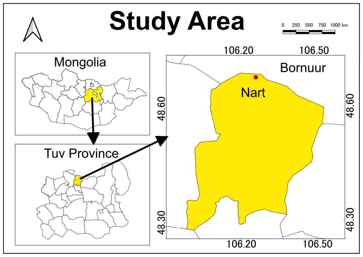
The study was done in Bornuur soum (district), Tuv Province, northern Mongolia, which is one of the country’s major wheat-producing regions. The study area is located approximately 115 km north of the capital Ulaanbaatar and lies at an elevation ranging from 1000 to 1500 m.a.s.l. (48.6794° N, 106.2672° E). Geographically, the area belongs to the transitional forest-steppe zone and is characterized by favorable conditions for both crop production and livestock husbandry. The study area is characterized by a continental semi-arid climate with cold, dry winters and warm summers. Air temperature typically ranges from −28 °C to 25 °C. The mean annual air temperature ranges between −2 and 0 °C. Annual precipitation varies between 250 and 300 mm, with more than 70% occurring during the summer months.

This seasonal concentration of precipitation has a deep impact on the pattern of crop growth and the dynamics of weed emergence in the region. The site area is part of the central agricultural zone of Mongolia and belongs to the long-term soil management and crop rotation experimental field of the agricultural research and training center “Nart Center” of Mongolian University of Life Sciences (Figure 1).

In the central agricultural region of Mongolia, most of the 361 vascular plant species have been recognized as arable land weeds [29]. At the Nart experimental site, weed surveys identified 18 weed species where annual weeds accounted for 61.1% of the total species, followed by perennials (33.3%) and biennials (5.6%) [7].

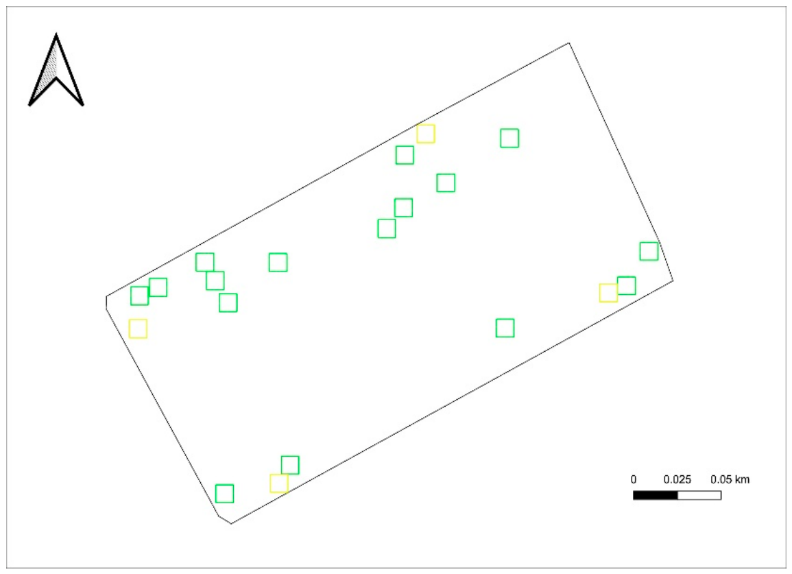
The study area was surveyed for spatial distribution of weed species in whole area. Observations from these plots were used to subsequently divide the field into 10 m × 10 m plots in annotation stage. A total of 20 plots were selected to ensure representative sampling of the heterogeneous weed distribution—some areas of the field had dense weed infestations while others were nearly weed-free. This plot-based approach allowed the preparation of a robust and spatially representative dataset for deep learning-based weed detection and segmentation (Figure 2).

2.2. UAV Data Collection and Image Processing

A Mavic 2 Pro UAV equipped with a Hasselblad L1D-20c camera (Victor Hasselblad-AB, Gothenburg, Sweden) acquired 20 mega pixel images. The camera sensor is a 1-inch CMOS with fixed focal length of 10 mm and aperture f/3.2. The images were acquired with 85% side and front overlap.

This setup resulted in a Ground Sampling Distance (GSD) of 0.37 cm/pixel. In addition, a high-precision GPS device was employed to ensure accurate coordinate measurements (GNSS, GPS + GLONASS). UAV images were acquired on 10 July 2025, combined with field survey data on weed spatial distribution with the GNSS. UAV flights were conducted over an area of 4 ha following routes designed in Drone Deploy version mobile 5.99.0 (Drone Deploy, San Francisco, CA, USA). The flight plan was set up at 15 m height from take-off points, nadir view, 3 m/s and shutter interval of 2 s. A total of eight GCPs were distributed across the field to ensure accurate georeferencing. During field surveys, 11 weed species belonging to nine families were identified within the study area. Among these, the three most abundant weed species were selected for analysis. The year 2025 was characterized by extremely dry conditions, which resulted in significantly reduced growth of wheat making weed identification comparatively easier during the survey period.

During the image processing stage, raw UAV imagery was processed using DJI Terra Agriculture 4.5 (SZ DJI Technology Co., Ltd., Shenzhen, China) to generate high-resolution RGB orthomosaic images. This orthomosaic was imported into QGIS (Open Source Geospatial Foundation, Beaverton, OR, USA), where weed was manually annotated and converted into vector-based datasets for DL training. The annotated weed was classified by species and assigned a class label for each. Variability in weed appearance and partial occlusion introduced minor annotation inconsistencies; however, training the models on heterogeneous and visually complex samples is expected to enhance their generalization capability under real-world field conditions. Although the manual annotation process is inherently subjective, restricting labels to confidently identifiable weed instances improved dataset robustness and reduced the risk of systematic bias. In some cases, discriminating weed in RGB imagery is not easy, particularly when species exhibit similar morphological characteristics or grow overlapped with other plants. In situ weed surveys were conducted, where weed species were visually identified, recorded, and documented. Proportional distribution of weed species ensures that the model is trained with representative data allowing robust and unbiased performance evaluation. 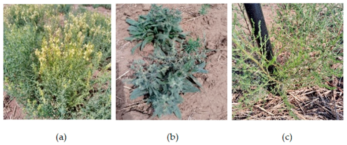L. buriatica, N. pulla and A. scoparia species were mainly selected for being the most abundant weed species within the study area in July (Figure 3).

During dataset annotation, the experimental area was divided into 16 plots (10 m × 10 m) used as the training dataset and 4 plots used as testing dataset (

Table 1. Annotated weed instance counts (individual plants) per species in the training and testing datasets.

Species	Training Annotation	Testing Annotation	Total
L. buriatica	3476	1211	4687
N. pulla	749	259	1008
A. scoparia	491	122	613
Total	4716	1592	6308

).

2.3. Image Pre-Processing and Augmentation

The 16 training plots were tiled into 512 by 512 pixels using a sliding window with no overlap. To keep the training and validation sets strictly independent, this non-overlapping approach was used. Overlapping tiles share pixel data and avoiding them prevents “data leakage” that would otherwise lead to overoptimistic accuracy results. The resulting tiles were split into 80% training and 20% validation using a fixed random seed to ensure full reproducibility. The four independent test plots were tiled separately at inference time using a different strategy. To increase training data diversity and improve model generalization, an offline augmentation strategy was applied exclusively to the training tiles using the Albumentations library [30]. Each training tile was augmented five times, yielding a training set five times larger than the original. Validation and test tiles were not augmented. Since individual weed plants are small relative to the 512 × 512 tile, most tiles contain instances of multiple species simultaneously, making class-specific augmentation impractical. The uniform five-fold augmentation therefore proportionally increases absolute instance counts for all three species, providing additional training signal for the two minority classes. All transforms were applied in a mask-aware manner to ensure geometric consistency between image and annotation.

The pipeline was organized into four steps (

Table 2. Augmentation pipeline applied to training tiles (Albumentations library).

Stage	Transform	Parameters	Purpose
Geometric	Horizontal flip	p = 0.50	Rotational invariance
	Vertical flip	p = 0.30	Rotational invariance
	Random rotate 90°	p = 0.50	Rotational invariance
	ShiftScaleRotate	shift ±0.08, scale ±0.25, rotate ±60°, p = 0.80	Viewpoint and scale variation
	Perspective	scale 0.05–0.15, p = 0.40	Sensor tilt/altitude variation
	RandomResizedCrop	512 × 512, scale 0.6–1.0, ratio 0.75–1.33, p = 0.50	Multi-scale weed appearance
Color/lighting	OneOf: BrightnessContrast/RandomGamma/CLAHE	p = 0.60	Illumination variation
	HueSaturationValue	hue ±8, sat ±15, val ±15, p = 0.50	Spectral variability
Blur/noise	OneOf: MotionBlur/GaussianBlur/GaussNoise	kernel ≤5/≤3/var 5–30, p = 0.30	Sensor noise and motion blur
Occlusion	CoarseDropout	2–6 patches, max 24 × 24 px, p = 0.40	Partial occlusion simulation

). First, geometric transforms were applied to simulate the same scene being captured by a UAV camera from different angles, scales and orientations. These included flips, rotations, shift–scale–rotate operations, perspective warping, and random cropping. Second, color and lighting transforms were added to account for changes in sunlight, shadows, and camera settings across different flight times. Each tile was randomized in brightness, contrast, gamma, hue and saturation. Third, some blurring or noise was introduced to simulate image degradation in the real world, due to sensor limitation or slight plant movement during flight. Finally, CoarseDropout was used to place random small black patches on some tiles to mimic the partial occlusion of plants by shadows or neighboring vegetation, so that the models can detect weeds even if they are not completely visible.

All built-in Ultralytics augmentations were explicitly disabled for YOLO26s-seg and RT-DETR-L to ensure the augmentation strategy was identical and fully controlled across all three models.

2.4. Model Training Configuration

All three models were trained under strictly identical conditions on a local workstation NVIDIA GeForce RTX 4070 Ti GPU (NVIDIA Corp, Santa Clara, CA, USA), 12 GB VRAM; Intel Core i9-13900K CPU (Intel Corporation, Santa Clara, CA, USA), 128 GB RAM; and Ubuntu 22.04.5 LTS (Canonical Ltd., London, UK) using Python 3.10.20 (Python Software Foundation, Wilmington, DE, USA). YOLO26s-seg and RT-DETR-L were trained within the Ultralytics framework; Mask R-CNN was trained using PyTorch 2.1.0 (PyTorch Foundation, San Francisco, CA, USA) and torch vision. All models used a batch size of 4, a maximum of 200 epochs, and early stopping with patience 50. Early stopping was triggered at epoch 72 for YOLO26s-seg, at epoch 63 for RT-DETR-L, and at epoch 74 for Mask R-CNN.

2.5. Deep Learning Models

Mask R-CNN (Mask Region-Based Convolutional Neural Network): Mask R-CNN is a two-stage instance segmentation framework that extends Faster R-CNN by incorporating a parallel branch for predicting segmentation masks for each ROI at the pixel level [23]. To extract spatially consistent features and guarantee accurate segmentation borders, this branch combines ROI Align [31]. Due to its high segmentation accuracy, Mask R-CNN has been widely applied in precision agriculture and remote sensing applications [32]. In this study, it was adopted as an accuracy-oriented baseline model for weed detection and segmentation.

YOLO26s-seg (You Only Look Once): It is the small segmentation variant of the YOLO26 family, a single-stage anchor-free and end-to-end detector that formulates object detection and instance segmentation as a unified task in a single forward pass. The YOLO26 models are designed for real-time applications, offering improved efficiency and faster inference, particularly on edge and low-power devices, without significant compromise in detection accuracy [26]. Its anchor-free design, NMS-free end-to-end architecture, and unified detection–segmentation pipeline make it particularly suitable for UAV-based agricultural monitoring [18]. According to its official GitHub (GitHub, San Francisco, CA, USA) documentation, YOLO26 is designed as a lightweight detector with a streamlined architecture that reduces computational complexity while maintaining competitive performance [33]. In UAV-based weed detection, where high-resolution orthomosaics often contain dense vegetation and small targets, such challenges are especially pronounced [23]. In this study, YOLO26s-seg was initialized with Ultralytics pre-trained weights and fine-tuned on the weed dataset [25].

RT-DETR-L (Real-Time Detection Transformar): Real-Time Detection Transformer is a transformer-based object detector from Ultralytics employing a hybrid CNN–transformer encoder–decoder architecture. Its self-attention mechanism models global contextual relationships across the full image, which can benefit detection in multi-species weed scenes with spatial co-occurrence and partial occlusion. RT-DETR-L uses a ResNet-50 backbone and outputs bounding box detections only—it does not produce instance segmentation masks. The model was initialized with Ultralytics pre-trained weights (rtdetr-l.pt) and fine-tuned on our weed dataset.

2.6. Comparison of Model Characteristics

The main purpose of this study is to detect weeds, more specifically, to reliably locate and identify the species of weeds in orthomosaics of UAVs for site-specific weed management in Mongolian wheat fields. The following three widely used deep learning models were selected based on their strong use and validation in agricultural remote sensing studies: Mask R-CNN, YOLO26s-seg, and RT-DETR-L. Although Mask R-CNN and YOLO26s-seg can produce pixel-level segmentation masks, they are also commonly used for object detection, and their bounding box outputs are suitable for weed mapping and spray-drone navigation. Their segmentation performance was additionally evaluated to determine whether pixel-level canopy mapping provides practical benefits for applications such as biomass estimation and crop growth monitoring. RT-DETR-L was included to examine whether transformer-based global context modeling can improve detection performance in the complex multi-species weed conditions found in Mongolian wheat fields. The main architectural features of the three models are summarized in

Table 3. Architectural comparison of the three DL models.

Feature	Mask R-CNN	YOLO26s-seg	RT-DETR-L
Architecture type	Two-stage, region-based	Single-stage, end to end	Transformer-based detector
Backbone	ResNet-50 + FPN	CSP-Muon (edge-optimized CNN)	ResNet-50
Detection head	RPN + RoIAlign + mask head	Decoupled	Hybrid encoder + decoder
Output	Boxes + instance masks	Boxes + instance masks	Bounding boxes only
Primary strength	Pixel-level mask accuracy	Speed + mask consistency	Global context modeling
Framework	PyTorch/torchvision	Ultralytics	Ultralytics

.

The comparative evaluation of Mask R-CNN, YOLO26s-seg, and RT-DETR-L enables a systematic analysis of the trade-offs between detection accuracy, segmentation quality, and inference speed under identical datasets and experimental conditions. While all models were trained under the same data pipeline and stopping criteria, the optimizer settings and learning rate schedules were individually tuned to reflect the recommended configurations for each architecture, ensuring that each model was given the best opportunity to perform to its full capability (

Table 4. Training hyperparameters for three DL models.

Hyperparameter	Mask R-CNN	YOLO26s-seg	RT-DETR-L
Input size	512 × 512	512 × 512	512 × 512
Max epochs	200	200	200
Early stopping patience	50	50	50
Actual stopping epoch	74	72	63
Batch size	4	4	4
Optimizer	AdamW	AdamW	AdamW
Initial learning rate (lr0)	0.0001	0.001	0.0001
Final LR factor (lrf)	-	0.01	0.01
LR scheduler	CosineAnnealingLR	Cosine decay (via lrf)	Cosine decay (via lrf)
Weight decay	0.0005	0.0005	0.0001
Warmup epochs	3	3	5
Pretrained weights	ImageNet (torchvision)	YOLO26s-seg (Ultralytics)	RT-DETR-L (Ultralytics)
Random seed	0	0	0
Built-in augmentation	Disabled	Disabled	Disabled

).

2.7. Evaluation

Since the main objective of this study is weed detection, model performance was first evaluated at the bounding box level using Precision (Equation (1)), Recall (Equation (2)), and F1-score (Equation (3)). In addition, mask-level evaluation was performed for YOLO26s-seg and Mask R-CNN to determine whether pixel-level segmentation provides practical advantages over bounding box detection for agricultural applications that require detailed canopy delineation. The metrics were calculated using true positives (TP), false positives (FP), and false negatives (FN):

$$\mathrm{P}\mathrm{r}\mathrm{e}\mathrm{c}\mathrm{i}\mathrm{s}\mathrm{i}\mathrm{o}\mathrm{n}={\displaystyle \frac{\mathrm{T}\mathrm{P}}{\mathrm{T}\mathrm{P}+\mathrm{F}\mathrm{P}}}$$

(1)

$$\mathrm{R}\mathrm{e}\mathrm{c}\mathrm{a}\mathrm{l}\mathrm{l}={\displaystyle \frac{\mathrm{T}\mathrm{P}}{\mathrm{T}\mathrm{P}+\mathrm{F}\mathrm{N}}}$$

(2)

$$\mathrm{F}1={\displaystyle \frac{2\left(\mathrm{P}\mathrm{r}\mathrm{e}\mathrm{c}\mathrm{i}\mathrm{s}\mathrm{i}\mathrm{o}\mathrm{n}\times \mathrm{R}\mathrm{e}\mathrm{c}\mathrm{a}\mathrm{l}\mathrm{l}\right)}{(\mathrm{P}\mathrm{r}\mathrm{e}\mathrm{c}\mathrm{i}\mathrm{s}\mathrm{i}\mathrm{o}\mathrm{n}+\mathrm{R}\mathrm{e}\mathrm{c}\mathrm{a}\mathrm{l}\mathrm{l})}}$$

(3)

Precision measures the proportion of predicted instances corresponding to actual weed plants (ability to avoid false detections) [34]. Recall (sensitivity), on the other hand, represents the proportion of correctly detected objects among all ground-truth positives, indicating the model’s capability to identify all relevant instances [35]. The F1-score is the harmonic mean of Precision and Recall, ranging from 0 to 1, where higher values indicate better performance [36]. All metrics are computed at the best-F1 confidence threshold for each model—the threshold that maximizes F1 across all confidence levels—rather than at a fixed shared threshold. This approach reflects the optimal operating point of each individual architecture and avoids artificially disadvantaging models that assign systematically lower confidence scores to true detections.

After training, each model was applied to the four testing plots. Rather than predicting on each plot as a single large image, inference was performed on 512 × 512 pixel tiles with 25% overlap (stride = 384 pixels) and the results were stitched back together into full-plot prediction maps. This tiled inference approach has the following two key advantages: it keeps the input size consistent with what the models were trained on, and the 25% overlap ensures that objects near tile boundaries are fully captured in at least one tile, reducing the border effect that commonly causes missed or incomplete detections in large-area UAV imagery.

Since each object can appear in more than one overlapping tile, the stitched predictions contain duplicate detections that need to be resolved before evaluation. To handle this, an Intersection over Smaller (IOS)-based Non-Maximum Merging (NMM) strategy was applied to all three models, as implemented in the SAHI framework [37]. For bounding boxes, the merged output is the minimum enclosing rectangle covering all grouped boxes. For the instance segmentation outputs (YOLO26s-seg and Mask R-CNN), the corresponding polygon masks were spatially unified using a geometric union operation, producing a single contiguous mask per detection. Unlike traditional suppression techniques that may discard partial detections at tile boundaries, the merging method maintains the full spatial integrity of each object. This prevents fragmented boundaries and ensures that predicted segments are reconstructed accurately across adjacent tiles.

Finally, the stitched and merged prediction maps were compared to the manually annotated ground truth polygons for quantitative evaluation. Evaluating model performance on stitched full-plot predictions provides a more realistic and robust measure of real-world detection capability. Tile level evaluation has two common limitations. First, objects near tile edges can be split across tiles. This can create incomplete detections that are counted as false negatives, even when the plant is correctly detected. Second, the same object may be detected in multiple overlapping tiles, which can increase the true positive count if duplicate detections are not removed before evaluation. By first merging overlapping predictions and then evaluating them against full plot ground truth polygons, each weed plant is counted only once. This provides a fair and spatially consistent evaluation and better reflects real UAV-based weed mapping performance. Beyond evaluation, this stitching and merging approach can also be applied to large areas. Any UAV orthomosaic can be divided into overlapping tiles, processed separately, and then merged into one seamless prediction map. The same pipeline can be used for any size fields. This makes the approach suitable for practical weed mapping at farm or landscape scale, where UAV imagery covers a large area.

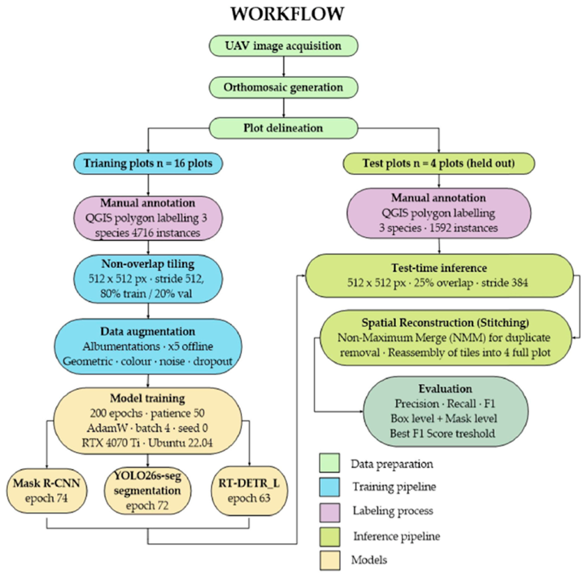
The complete workflow, from UAV image acquisition through model training, tiled inference, prediction stitching, and performance evaluation, is illustrated in (Figure 4).

3. Results

Three deep learning models—YOLO26s-seg, Mask R-CNN, and RT-DETR-L—were evaluated on four independent test plots containing 1592 annotated weed instances across the following three species: L. buriatica (1211), N. pulla (259), and A. scoparia (122) (

Table 5. Per-class bounding box detection metrics for all three models.

Model	Species	TP	FP	FN	Precision	Recall	F1-Score
YOLO26s-seg	L. buriatica	725	420	486	0.633	0.599	0.615
	N. pulla	200	152	59	0.568	0.772	0.655
	A. scoparia	38	67	84	0.362	0.311	0.335
Mask R-CNN	L. buriatica	883	658	328	0.573	0.729	0.642
	N. pulla	175	182	84	0.490	0.676	0.568
	A. scoparia	12	13	110	0.480	0.098	0.163
RT-DETR-L	L. buriatica	913	511	298	0.641	0.754	0.693
	N. pulla	175	107	84	0.621	0.676	0.647
	A. scoparia	21	10	101	0.677	0.172	0.275

).

3.1. Performance of Mask R-CNN

At the bounding box level, Mask R-CNN showed the best detection performance for L. buriatica, with a Precision of 0.573, Recall of 0.729, and F1-score of 0.642. The model correctly detected many instances (TP = 883), although false positives (FP = 658) and false negatives (FN = 328) were also relatively high. For N. pulla, the model achieved a Precision of 0.490 and Recall of 0.676, resulting in an F1-score of 0.568. Higher Recall but lower Precision indicates that truest instances were detected, but many false positives were also produced (FP = 182). A. scoparia showed the weakest bounding box detection performance, with a Precision of 0.480, Recall of 0.098, and F1-score of 0.163, indicating that most individuals were missed.

3.2. Performance of YOLO26s-seg

At the bounding box level, YOLO26s-seg showed strong detection performance across all species. For L. buriatica, the model achieved a Precision of 0.633, Recall of 0.599, and F1-score of 0.615. The model detected many true instances (TP = 725), although the number of false negatives (FNs = 486) remained relatively high. For N. pulla, YOLO26s-seg achieved the highest Recall among all three models at 0.772, with an F1-score of 0.655. Precision 0.568 indicates that the model was highly sensitive to this species but also produced more false positives. For A. scoparia, YOLO26s-seg achieved an F1-score of 0.335, which was the highest among all tested models for this species.

3.3. Performance of RT-DETR-L

RT-DETR-L demonstrated the strongest overall detection performance among the evaluated models. For L. buriatica, it achieved the highest metrics, with a Precision of 0.641, Recall of 0.754, and an F1-score of 0.693. The model also detected the highest number of true positives (TPs = 913) while maintaining a relatively low number of false positives (FPs = 511), reflecting improved discriminative capability.

For N. pulla, RT-DETR-L achieved a Precision of 0.621, Recall of 0.676, and an F1-score of 0.647, representing a more balanced trade-off between Precision and Recall compared to YOLO26s-seg, which exhibited higher Precision but lower Recall. Additionally, the lower number of false positives (FPs = 107, compared to 182 for Mask R-CNN) indicates improved detection reliability.

A. scoparia remained the most challenging species for RT-DETR-L, with a Precision of 0.677 and Recall of 0.172 (F1 = 0.275). Although these values are slightly higher than those of the other models, overall detection performance for this species remained limited. The consistently low Recall across all models suggests that the difficulty is primarily due to insufficient training data rather than model-specific limitations.

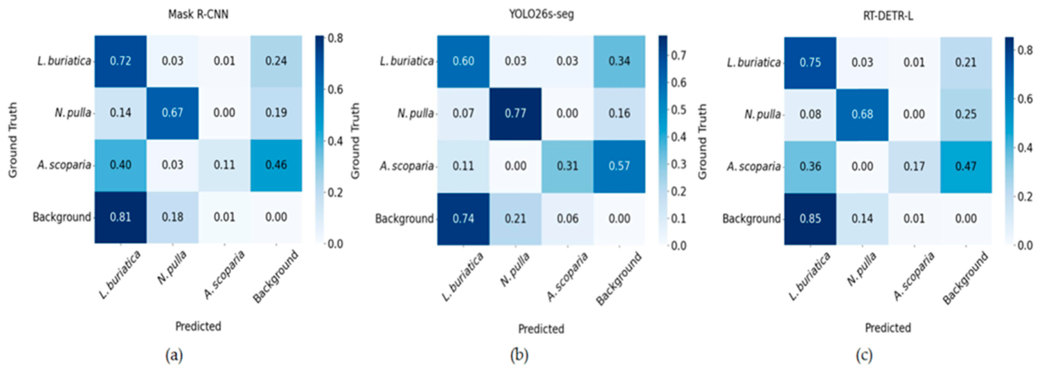
The normalized confusion matrices for all three models at the bounding box level (IoU = 0.5) are row normalized, such that diagonal values represent per-class Recall (Figure 5). The consistently low diagonal values for A. scoparia across all models visually confirm its detection difficulty, while off-diagonal elements indicate a tendency to misclassify background regions as L. buriatica.

3.4. Performance of Mask R-CNN and YOLO26-seg

At the mask level, Mask R-CNN performance for L. buriatica improved slightly, with Precision increasing to 0.607, Recall of 0.722 and F1-score to 0.659. This suggests that the predicted masks were better aligned with actual canopy boundaries, even when bounding boxes were not perfectly positioned. For N. pulla, mask-level Precision improved to 0.545, Recall of 0.668 and the F1-score increased to 0.600. This indicates that although bounding box predictions were overestimated, many corresponding masks were geometrically more accurate. For A. scoparia, mask-level performance remained weak, with a Precision of 0.500, Recall of 0.109, and F1-score of 0.179, which was consistent with the bounding box detection results.

At the mask level, YOLO26s-seg produced similar results like bounding box performance across all species. For L. buriatica, the model achieved a Precision of 0.631 and F1-score of 0.613. For N. pulla, Recall reached 0.776 and the F1-score was 0.658, which is consistent with the bounding box results. For A. scoparia, F1-score was 0.326. The small differences between bounding box and mask metrics indicate that YOLO26s-seg masks were well-aligned with the detected object boundaries (

Table 6. Per-class instance segmentation mask metrics for YOLO26s-seg and Mask R-CNN models.

Model	Species	TP	FP	FN	Precision	Recall	F1-Score
YOLO26s-seg	L. buriatica	722	423	489	0.631	0.596	0.613
	N. pulla	201	151	58	0.571	0.776	0.658
	A. scoparia	37	68	85	0.352	0.303	0.326
Mask R-CNN	L. buriatica	806	523	310	0.607	0.722	0.659
	N. pulla	169	141	84	0.545	0.668	0.600
	A. scoparia	12	12	98	0.500	0.109	0.179

).

3.5. Inference Performance

To assess the deploy ability of all three models, a controlled inference benchmark was conducted on the same testing set of 512 × 512 images. All models were evaluated at batch size = 1 on a single NVIDIA RTX 4070 Ti GPU (NVIDIA Corp, Santa Clara, CA, USA) using PyTorch 2.6.0 and CUDA 12.4. Average latency was measured over 500 forward passes after a 10-image warm-up period. GPU memory was recorded via PyTorch’s memory allocator. YOLO26s-seg achieved 5.67 ms per image (176.3 FPS) with 304 MB GPU memory. It is faster than RT-DETR-L and Mask R-CNN. RT-DETR-L achieved 18.56 ms per image (53.9 FPS) with 430 MB memory. Mask R-CNN was the slowest model at 26.27 ms per image (38.1 FPS) and required 1605 MB of GPU memory.

4. Discussions

4.1. Overall Detection Performance

Mask R-CNN produced competitive results for L. buriatica and showed a notable pattern. Its mask-level F1-score (0.659) exceeded its box-level score (0.642) for this species, which reflects the strength of its two-stage RoI Align mechanism in creating accurate pixel-level masks. However, the model produced substantially more false positives for N. pulla (182 at the box level and 141 at the mask level) compared to the other two models. This high false positive rate is consistent with the known tendency of region-based detectors to produce erroneous detections in complex agricultural environments, where background vegetation and crop residues may resemble weed canopy structures. Such limitations of region-based detectors in dense agricultural scenes have been reported previously [38].

Performance metrics were computed at the best-F1 confidence threshold for each model. The thresholds were 0.15 for YOLO26s-seg, 0.45 for RT-DETR-L, and 0.60 for Mask R-CNN. These differences reflect variations in confidence score distributions across models, a well-known characteristic of deep neural networks and object detectors [39].

YOLO26s-seg showed competitive performance. For N. pulla, it achieved the highest Recall among all three models at both box (0.772) and mask (0.776) levels. This means the model detected more true instances of this species than any other model. However, Precision was lower (0.568), so more false positives were also included. For A. scoparia, YOLO26s-seg showed an F1-score of 0.335, which is the best result for this species across all models. This suggests the newer architecture handles minority class detection better, likely through improved feature learning in the end-to-end framework.

RT-DETR-L achieved the strongest detection performance for L. buriatica, the most dominant and agronomical important weed species in the study area. With a Precision of 0.641, Recall of 0.754, and an F1-score of 0.693, it outperformed both YOLO26s-seg and Mask R-CNN for this class. It also showed the highest true positive count (TP = 913) while keeping false positives relatively low (FPs = 511). This performance may be because of its transformer-based architecture, which uses self-attention to capture global contextual relationships in complex UAV imagery [22]. This is especially advantageous when weed plants overlap and are distributed across spatially heterogeneous backgrounds typical of UAV imagery [40,41]. For N. pulla, RT-DETR-L also showed a well-balanced result (F1 = 0.647) which is very close to YOLO26s-seg. Also, it has lowest false positive count among all models for this species (FP = 107). For A. scoparia, detection remained limited (F1 = 0.275), which is consistent with the class imbalance challenge shared by all three models rather than a model-specific weakness.

Among the models, RT-DETR showed slightly improved performance, likely due to its ability to consider global image context rather than relying only on local features. This advantage of transformer-based models has been widely highlighted in recent studies due to their ability to model long-range dependencies and capture global contextual relationships [41]. Overall, RT-DETR-L is the most reliable model for detecting the dominant weed species and is recommended for detection-focused applications such as weed scouting and spray-drone guidance.

4.2. Segmentation Mask Quality

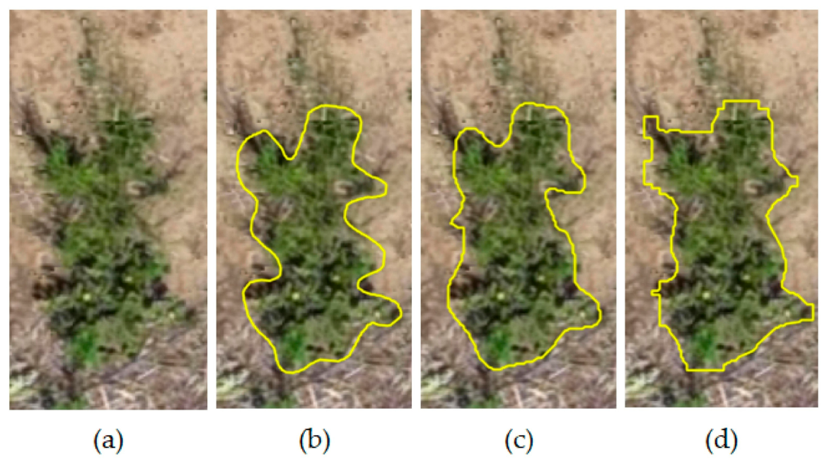
Beyond detection metrics, the quality of predicted instance masks is critical for applications requiring spatial delineation of individual weed plants. Qualitative inspection of the predicted masks revealed clear differences between YOLO26s-seg and Mask R-CNN. Mask R-CNN consistently produced better masks that are closer to the followed actual canopy boundary of individual plants. This happens because Mask R-CNN uses the RoI Align operation in its second stage. It resizes feature maps to a fixed size before predicting masks. This helps preserve small spatial details that are often lost in single-stage models. YOLO26s-seg produced tighter and more consistent masks overall. However, it sometimes created slightly smoother or more generalized boundaries for plants with complex shapes (Figure 6).

4.3. Class Imbalance and Detection of Artemisia scoparia

A. scoparia was consistently the most difficult species to detect for all three models, with F1-scores ranging from 0.163 (Mask R-CNN box) to 0.275 (RT-DETR-L box) and Recall values as low as 0.098. This poor performance was mainly caused by strong class imbalance in the training dataset. A. scoparia had only 491 annotated training samples, while L. buriatica had 3476 samples, which is about a 7:1 ratio. Although five-fold offline augmentation was applied equally to all classes, the total number of A. scoparia samples was still too low to learn strong features for this species. This problem was clearly visible in the confusion matrices of all three models (Figure 5). In many cases, A. scoparia plants were wrongly classified as background or as L. buriatica.

It is important to note that A. scoparia was not only underrepresented in the training dataset but was also the least common species in the field. This reflects its naturally low presence in the study area. Its thin leaves, scattered canopy structure, and low contrast with the dry soil background made detection more difficult at the 0.379 cm/pixel GSD used in this study. As a result, the lower detection performance for this species has limited practical impact on weed management. Field control decisions are mainly based on the dominant weed species, while A. scoparia represents only a small part of the total weed population. If this species becomes more common in future seasons or in other fields, collecting more samples and applying class-specific augmentation would likely improve model performance within the current framework. The impact of incomplete or imperfect annotations on model evaluation has been widely discussed in remote sensing studies, where weak or partial labels can introduce bias in performance assessment [42]. Finally, it should be noted that this study is limited to a single UAV acquisition condition and RGB imagery. Future work should explore multi-temporal datasets, higher-resolution imagery, and multispectral data to improve detection robustness and generalization [43].

4.4. Challenges in Detection Accuracy and Directions for Improvement

While the models showed meaningful detection capability for the dominant species, several systematic challenges affected the results.

The most consistent issue across all three models was misclassification of background regions as L. buriatica. This reflects a real field condition rather than a model failure alone. L. buriatica was the dominant species and was present across nearly the entire field. In many areas of the orthomosaic, sparse or recently emerged plants blended with the dry soil background. The models learned this dominance pattern and tended to predict L. buriatica in uncertain regions. This explains why background to L. buriatica confusion is the most common pattern in all three confusion matrices. A related challenge is annotation incompleteness for L. buriatica. Many small individuals could not be annotated because they occupied only a few pixels at the 0.379 cm/pixel GSD. These unannotated instances were treated as false positives in the evaluation, lowering the Precision values.

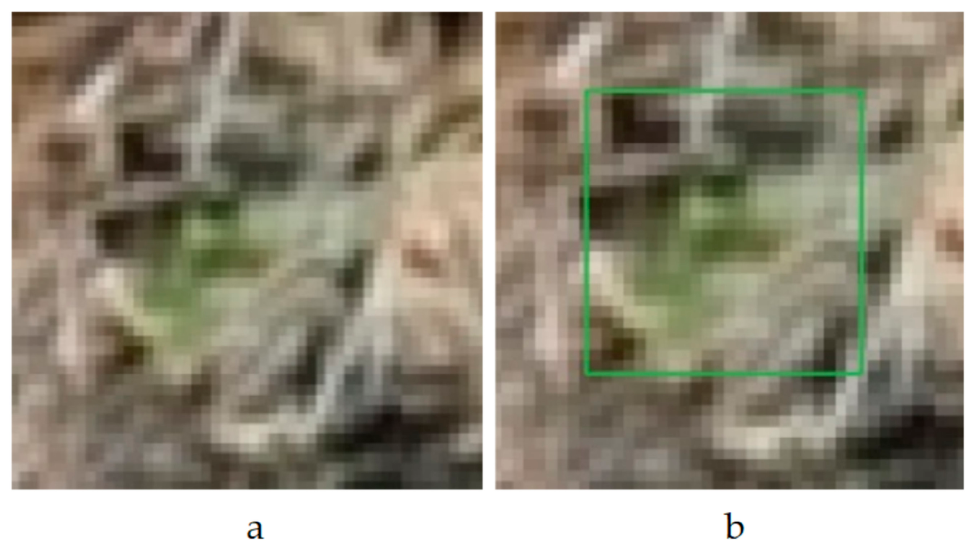
A consistent observation across all three models, and most clearly in RT-DETR-L, was the detection of weed instances absent from the ground truth annotation. Qualitative inspection shows that many of these correspond to very small L. buriatica seedlings that could not be annotated because of the lower resolution (Figure 7).

This means the reported Precision values are conservative estimates rather than true measures of model capability. The models likely detect real weeds that the annotator could not confirm. Despite this limitation, detecting small seedlings at early stage is very useful. Identifying dense patches of early-stage L. buriatica before they develop is more valuable than missing them, even if counts cannot be verified from the ground truth [35]. The main way to address these challenges is to use higher resolution imagery. Higher resolution images could make small seedlings easier to see and annotate, leading to more complete ground truth labels and more accurate evaluation. Ground-level validation surveys immediately after UAV flights would provide a more complete reference for evaluation. Targeted data collection during early crop growth stages would also improve training data quality for minority classes. Together, these improvements would reduce the incomplete annotations that currently affect both model training and performance evaluation.

4.5. Practical Implications for Weed Management

The results of this study demonstrate that all three models can effectively detect weed species in UAV orthomosaics, and their differences in accuracy, mask quality, and inference speed make them suitable for different stages of a precision weed management workflow.

In precision agriculture, spray drones target weed-infested zones rather than individual plants. Spraying covers, a broad area around the detection centroid and herbicides do not damage crops immediately. Pixel-perfect mask accuracy is therefore not always required. Missing a weed is costlier than a false detection, because an undetected weed can grow, compete with the crop, and produce seeds. High Recall is generally more important than high Precision for spray-based applications.

RT-DETR-L achieved the highest Recall for the dominant species. It is recommended for detection-based scouting and spray-drone guidance. Since spray drones follow centroid coordinates rather than polygon boundaries, its bounding box output is sufficient and the absence of mask output is not a limitation. YOLO26s-seg achieved the highest Recall for N. pulla and the best detection of A. scoparia among all models. This makes it well-suited for applications where detection completeness across all species matters, such as GIS-based weed density mapping and variable-rate herbicide planning. Its consistent box-to-mask performance also makes the segmentation output reliable for generating vector polygon layers for GIS workflows. Mask R-CNN is most appropriate for tasks that require accurate canopy boundary delineation, such as weed biomass estimation and growth stage monitoring.

The current workflow runs on a ground station computer after UAV image acquisition. Results are transferred to the spray drone as georeferenced waypoints or spray maps. Real-time inference is a goal for future development. YOLO26s-seg achieved 5.67 ms per image with 304 MB memory, making it fast and lightweight enough for future edge deployment on UAV-mounted hardware. RT-DETR-L (18.56 ms, 430 MB) and Mask R-CNN (26.27 ms, 1605 MB) are both suitable for ground station use, with RT-DETR-L being much more memory-efficient.

Future research should focus on diversifying the training dataset with minority species and utilizing higher-resolution or multispectral imagery to improve early-stage weed identification. Additionally, multi-temporal data acquisition could capture emergence dynamics to refine intervention timing. The tiled inference and IOS-based NMM stitching pipeline scales to fields of any size and provides a practical foundation for operational weed mapping at the farm level.

5. Conclusions

This study compared three deep learning models, YOLO26s-seg, Mask R-CNN, and RT-DETR, for UAV-based weed detection and segmentation in wheat fields. The models were selected based on their wide adoption in agricultural remote sensing research, with the primary goal of identifying which best serves the practical weed detection and mapping needs of Mongolian dryland wheat production. This is the first such evaluation under Mongolian agro-ecological conditions. All three models successfully detected the dominant weed species, although their performance varied by model design and task.

RT-DETR-L achieved the highest detection accuracy across the dominant species, confirming the strength of transformer-based models in capturing global image context. Mask R-CNN produced the most accurate canopy boundary delineation at the mask level, particularly for morphologically complex plants, but generated more false positives in cluttered field conditions. YOLO26s-seg showed well-rounded and competitive performance. It achieved the highest Recall for N. pulla among all models and the best F1-score for A. scoparia. Its consistent box-to-mask agreement and NMS-free end-to-end design make it efficient and reliable for both detection and segmentation tasks. With 5.67 ms inference time and 304 MB memory, it is also the most suitable model for future edge deployment.

A clear limitation of this study was the low detection performance for A. scoparia for all three models. This was mainly caused by class imbalance, along with the small size and less distinctive appearance of this species in UAV imagery. Since it is a naturally sparse occurrence in the field, this has minimal practical impact on weed management. The models also consistently detected small weed seedlings absent from the ground truth. This suggests that the reported precision values may be slightly underestimated. From a practical point of view, the choice of model depends on the intended application. RT-DETR-L is most suitable for weed counting and spray-drone guidance. YOLO26s-seg works well for GIS-based mapping and variable-rate herbicide application where detection completeness across all species is important. Mask R-CNN is best for tasks requiring detailed canopy delineation such as biomass estimation and growth stage monitoring.

These findings are particularly relevant for wheat production in Mongolia, where semi-arid conditions, low crop density, and heterogeneous soil backgrounds make weed detection a really challenging task. The results demonstrate that established deep learning models can be effectively applied in this regional context and provide a practical foundation for precision weed management in Mongolia and similar dryland agricultural environments. Future work should focus on collecting more data for underrepresented species and using higher-resolution or multispectral imagery. Multi-temporal data may also improve detection by capturing weed growth dynamics over the season. In addition, future studies could evaluate newer model architectures, which would further increase the value of the work for the research community.