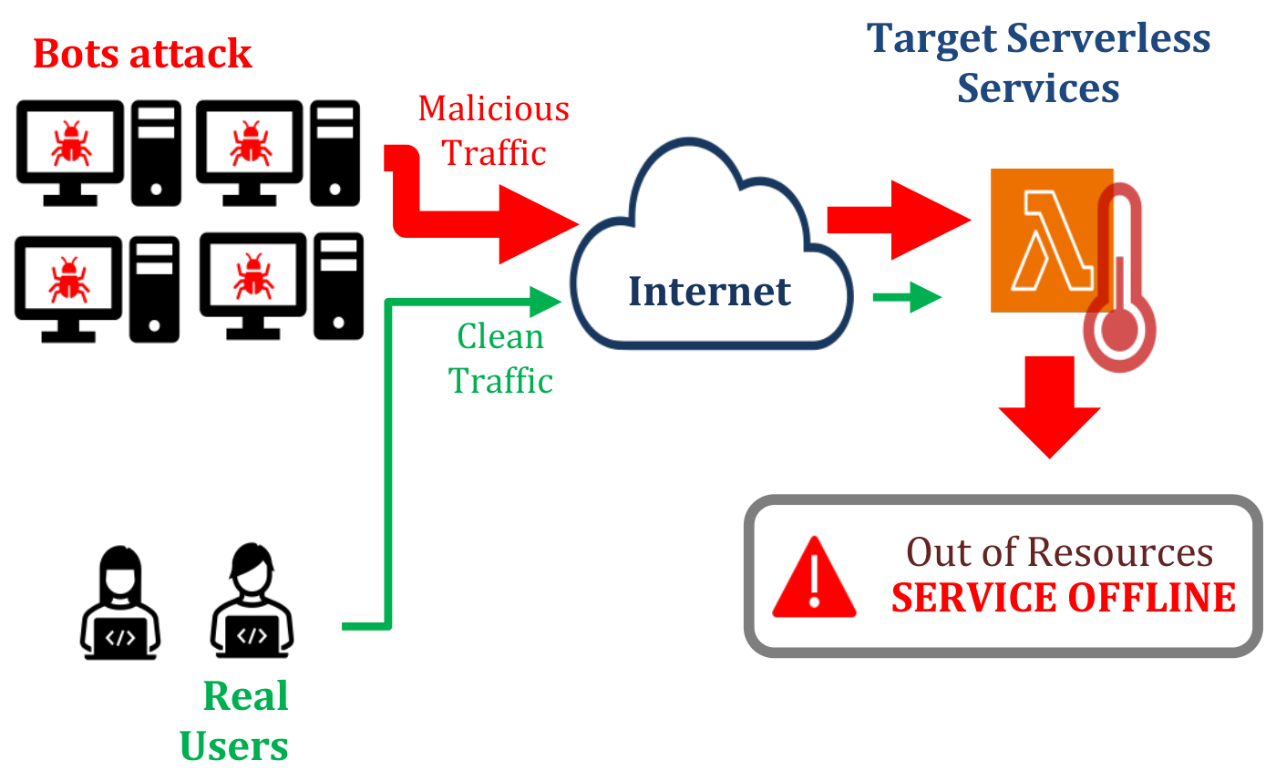
Figure 1.
Schematic representation of a typical distributed denial of service (DDoS) attack. Bot-infected machines generate malicious traffic that, combined with legitimate user traffic, reaches the target serverless service via the Internet. The resulting resource exhaustion causes the service to go offline.
Figure 1.
Schematic representation of a typical distributed denial of service (DDoS) attack. Bot-infected machines generate malicious traffic that, combined with legitimate user traffic, reaches the target serverless service via the Internet. The resulting resource exhaustion causes the service to go offline.
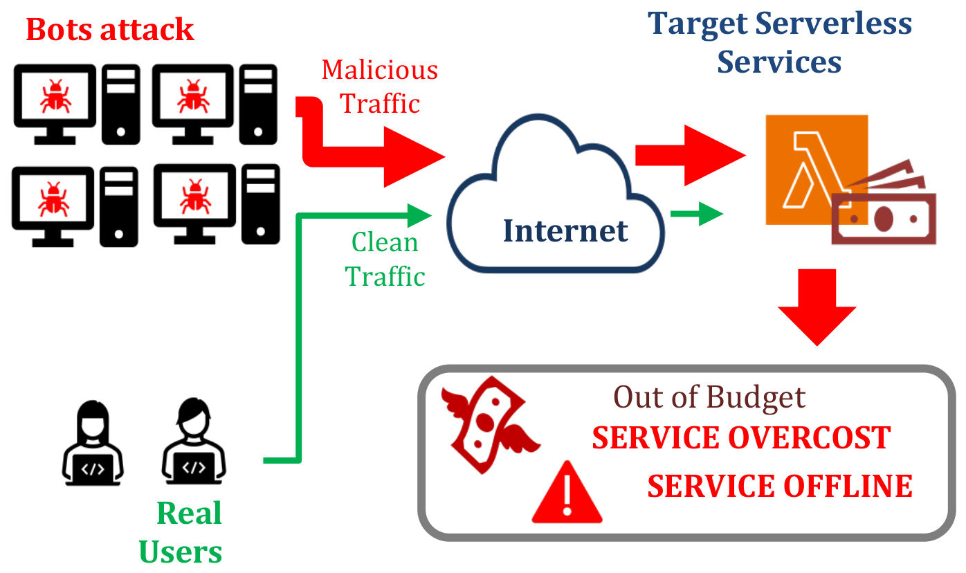
Figure 2.
Schematic representation of a typical denial of wallet (DoW) attack in a serverless environment. Bot traffic and legitimate user traffic reach the target serverless service through the Internet. Unlike DDoS, the attack does not necessarily interrupt availability but instead exhausts the billing budget, resulting in service overcost and potentially driving the service offline.
Figure 2.
Schematic representation of a typical denial of wallet (DoW) attack in a serverless environment. Bot traffic and legitimate user traffic reach the target serverless service through the Internet. Unlike DDoS, the attack does not necessarily interrupt availability but instead exhausts the billing budget, resulting in service overcost and potentially driving the service offline.
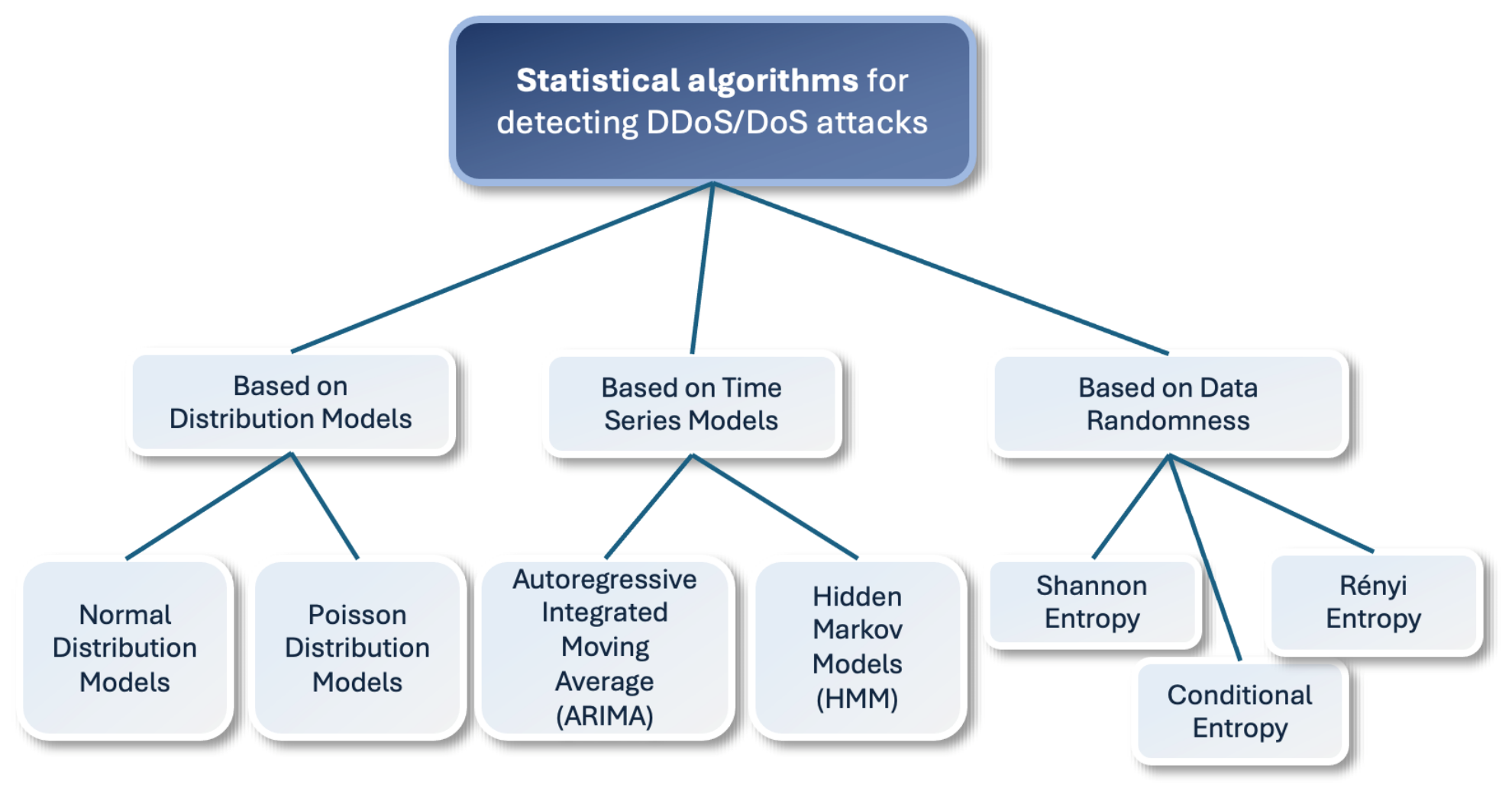
Figure 3.
Taxonomy of statistical algorithms for detecting DDoS/DoW attacks, classified into three main categories.
Figure 3.
Taxonomy of statistical algorithms for detecting DDoS/DoW attacks, classified into three main categories.
Figure 4.
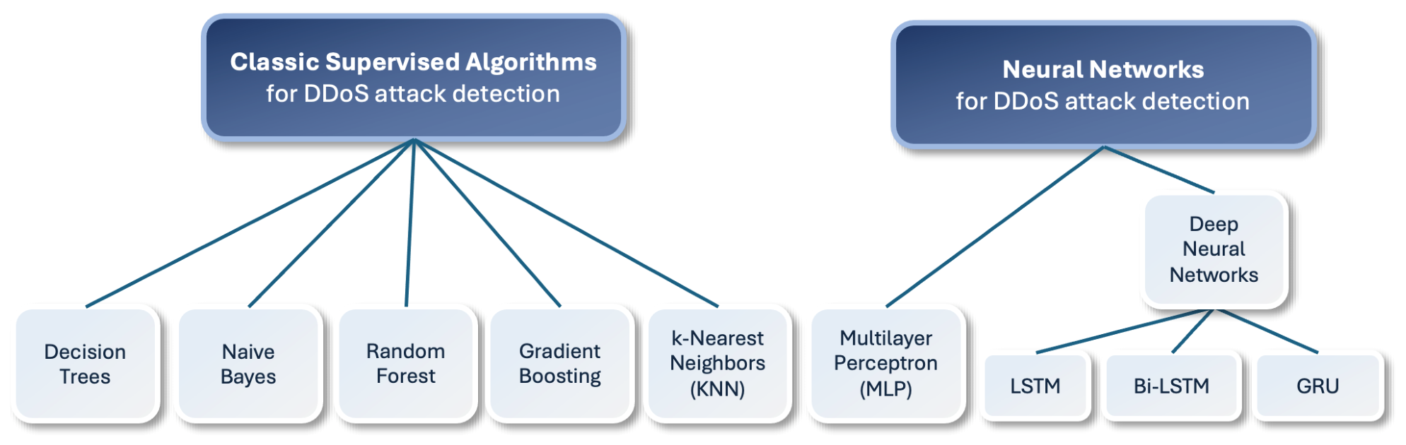
Taxonomy of machine learning (ML) and neural network (NN) algorithms employed for DDoS/DoW attack detection.
Figure 4.
Taxonomy of machine learning (ML) and neural network (NN) algorithms employed for DDoS/DoW attack detection.
Figure 5.
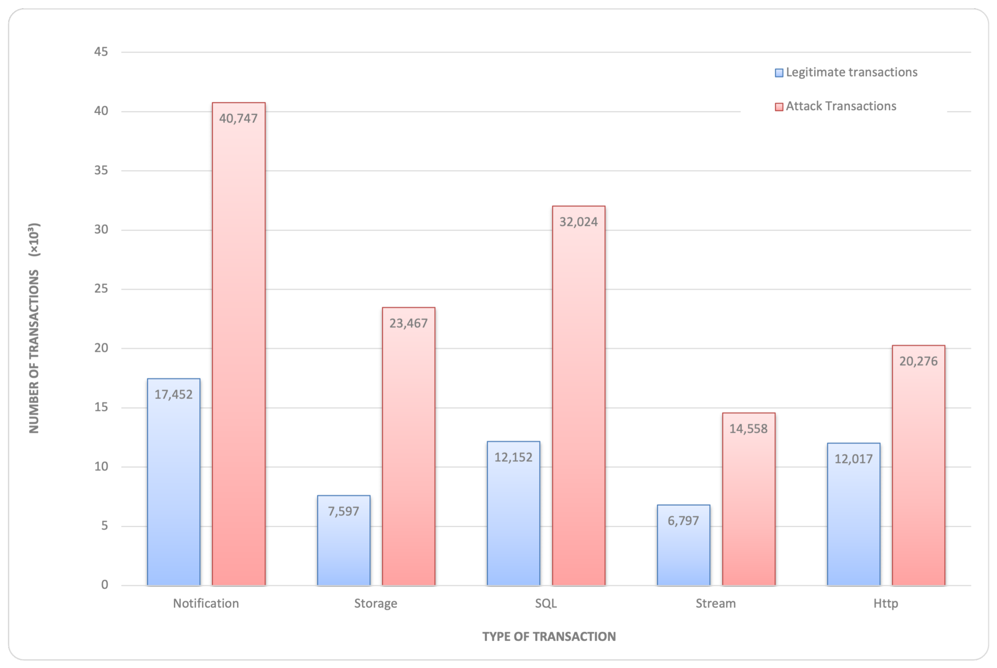
Distribution of legitimate (blue) and attack (red) transactions across the five event types present in the dataset: notification, storage, SQL, stream, and HTTP. In all categories, legitimate traffic exceeds attack traffic, with the notification type showing the highest volume of legitimate transactions (40,747) and the HTTP type showing the highest proportion of attack transactions (20,276).
Figure 5.
Distribution of legitimate (blue) and attack (red) transactions across the five event types present in the dataset: notification, storage, SQL, stream, and HTTP. In all categories, legitimate traffic exceeds attack traffic, with the notification type showing the highest volume of legitimate transactions (40,747) and the HTTP type showing the highest proportion of attack transactions (20,276).
Figure 6.
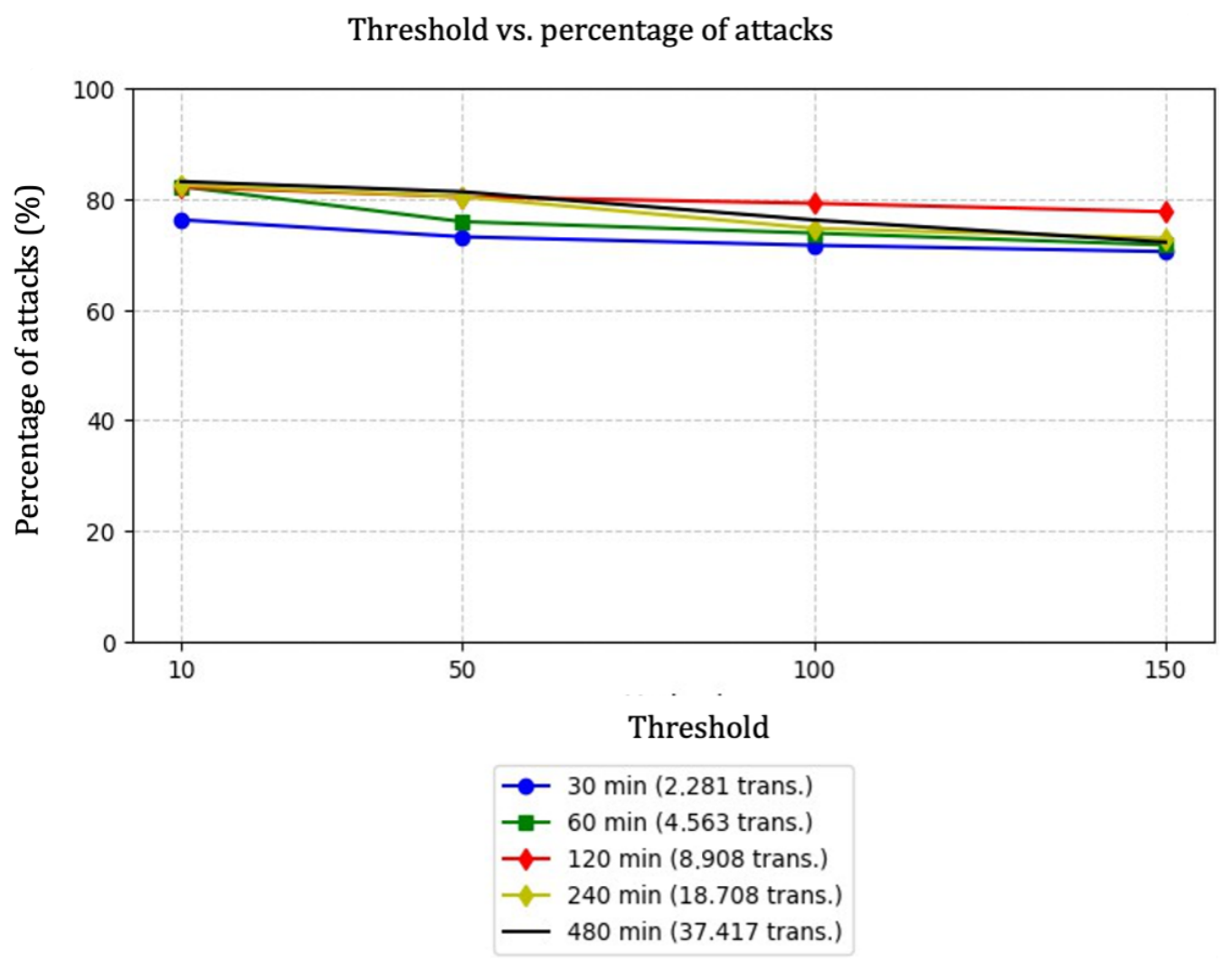
Relationship between the detection threshold value and the percentage of transactions flagged as suspected attacks, plotted for five different analysis window sizes (30, 60, 120, 240, and 480 min). As the threshold increases, the percentage of suspected attack transactions decreases across all window sizes.
Figure 6.
Relationship between the detection threshold value and the percentage of transactions flagged as suspected attacks, plotted for five different analysis window sizes (30, 60, 120, 240, and 480 min). As the threshold increases, the percentage of suspected attack transactions decreases across all window sizes.
Figure 7.
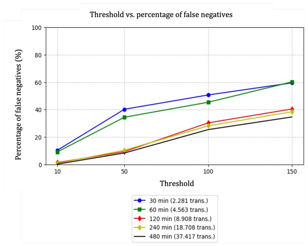
Relationship between the threshold value and the percentage of false negatives for five window sizes (30, 60, 120, 240, and 480 min). Higher threshold values result in increased false negative rates. The optimal configuration identified is a window size of 480 min with a threshold of 10, yielding a false negative rate of 0.44% and an attack detection rate of 83.08%.
Figure 7.
Relationship between the threshold value and the percentage of false negatives for five window sizes (30, 60, 120, 240, and 480 min). Higher threshold values result in increased false negative rates. The optimal configuration identified is a window size of 480 min with a threshold of 10, yielding a false negative rate of 0.44% and an attack detection rate of 83.08%.
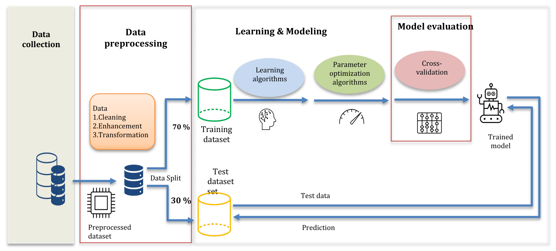
Figure 8.
Schematic overview of the supervised learning pipeline applied in this study. The process comprises five sequential stages: (1) data collection, (2) data preprocessing (cleaning, enhancement, and transformation), (3) data splitting into training (70%) and test (30%) sets, (4) learning and modeling (including cross-validation and parameter optimization), and (5) model evaluation on test data to produce the trained model.
Figure 8.
Schematic overview of the supervised learning pipeline applied in this study. The process comprises five sequential stages: (1) data collection, (2) data preprocessing (cleaning, enhancement, and transformation), (3) data splitting into training (70%) and test (30%) sets, (4) learning and modeling (including cross-validation and parameter optimization), and (5) model evaluation on test data to produce the trained model.
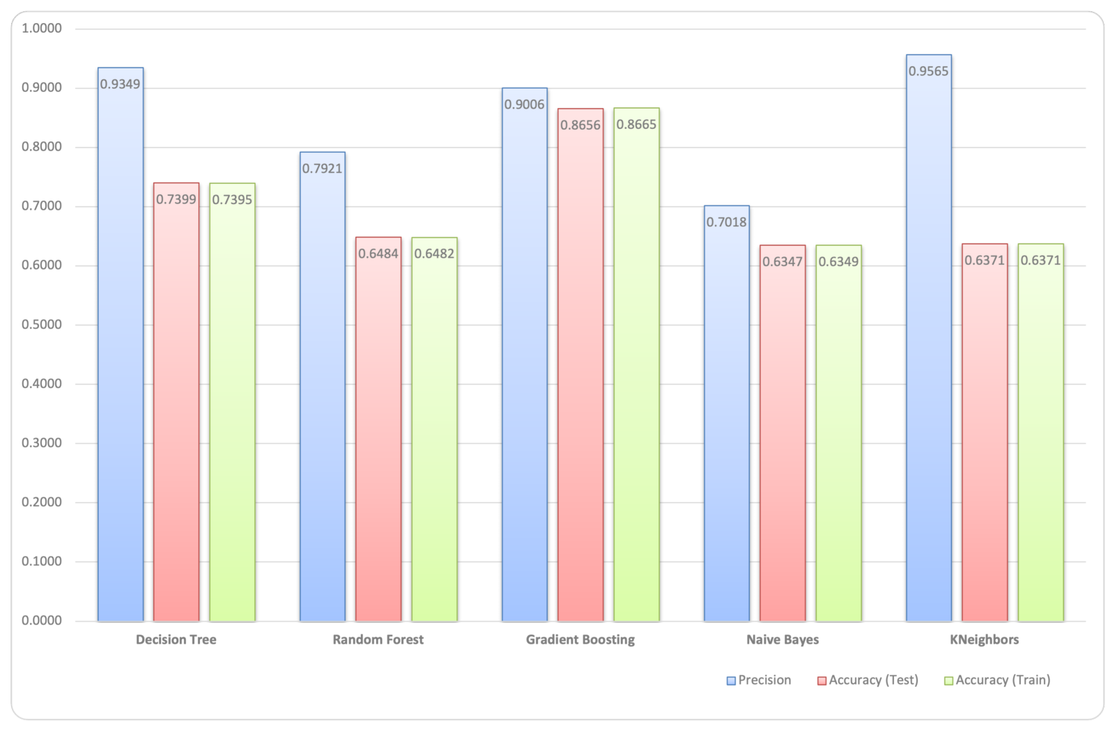
Figure 9.
Performance comparison of five classical machine learning algorithms (decision tree, random forest, gradient boosting, naïve Bayes, and k-nearest neighbors) on the DoW detection dataset. Three metrics are reported for each algorithm: precision (blue), accuracy on test data (red), and accuracy on training data (green). The best precision is achieved by KNN (0.956) and the best test accuracy by gradient boosting (0.865).
Figure 9.
Performance comparison of five classical machine learning algorithms (decision tree, random forest, gradient boosting, naïve Bayes, and k-nearest neighbors) on the DoW detection dataset. Three metrics are reported for each algorithm: precision (blue), accuracy on test data (red), and accuracy on training data (green). The best precision is achieved by KNN (0.956) and the best test accuracy by gradient boosting (0.865).
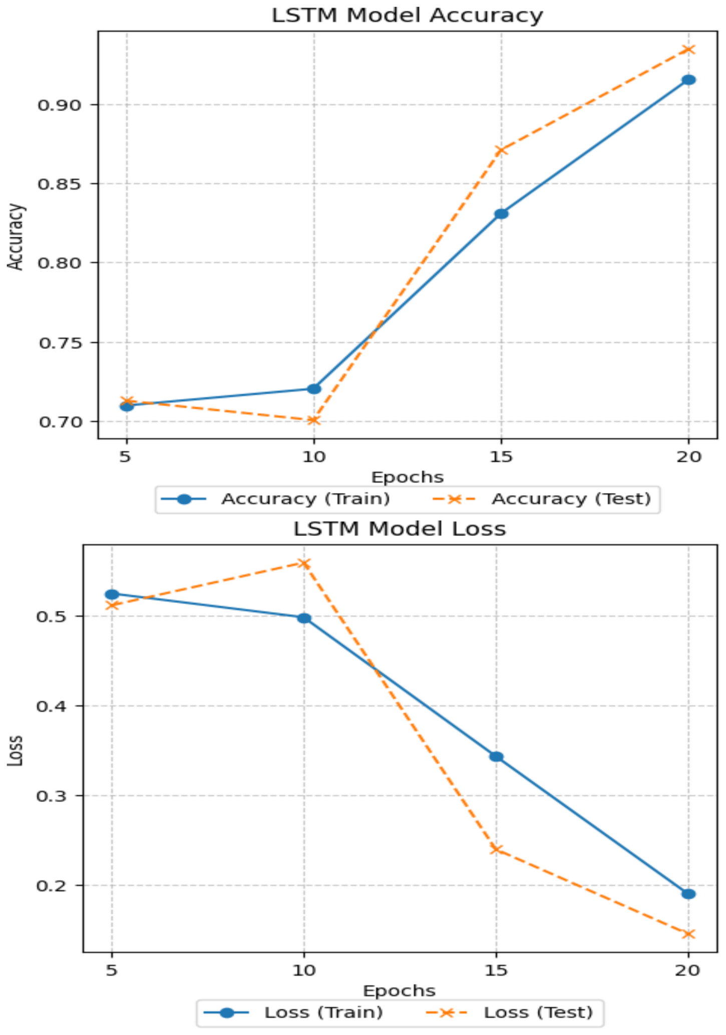
Figure 10.
Training and test performance of the LSTM model over 20 epochs. (top) Accuracy curves for training (solid line) and test (dashed line) sets, showing a progressive increase from approximately 0.70 to 0.90. (down) Loss curves for training and test sets, showing a decline from approximately 0.50 to 0.20, confirming that the model learns effectively and generalizes without overfitting.
Figure 10.
Training and test performance of the LSTM model over 20 epochs. (top) Accuracy curves for training (solid line) and test (dashed line) sets, showing a progressive increase from approximately 0.70 to 0.90. (down) Loss curves for training and test sets, showing a decline from approximately 0.50 to 0.20, confirming that the model learns effectively and generalizes without overfitting.
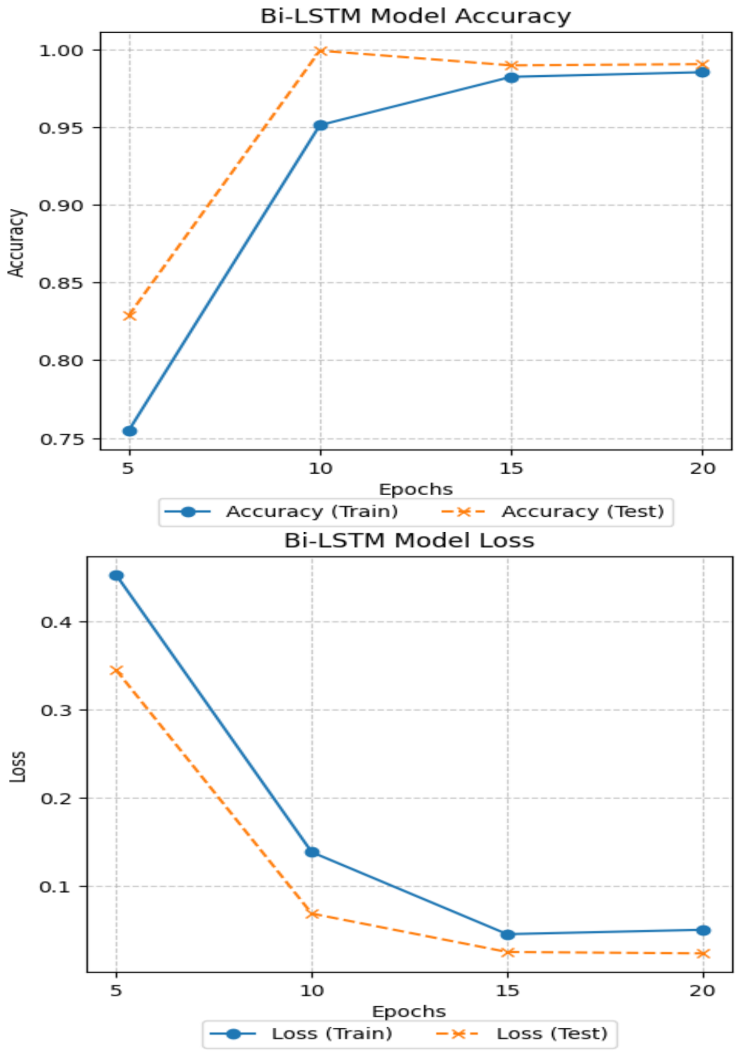
Figure 11.
Training and test performance of the Bi-LSTM model over 20 epochs. (top) Accuracy curves, showing rapid convergence to values close to 1.00 on both training and test sets. (down) Loss curves, showing a sharp decline from approximately 0.40 to below 0.10, indicating strong generalization. The optimal epoch count was determined to be 20, beyond which no significant improvement was observed.
Figure 11.
Training and test performance of the Bi-LSTM model over 20 epochs. (top) Accuracy curves, showing rapid convergence to values close to 1.00 on both training and test sets. (down) Loss curves, showing a sharp decline from approximately 0.40 to below 0.10, indicating strong generalization. The optimal epoch count was determined to be 20, beyond which no significant improvement was observed.
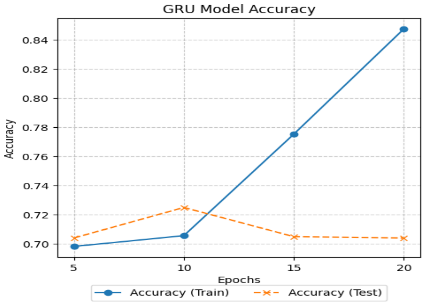
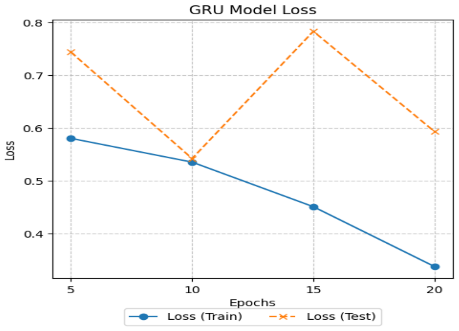
Figure 12.
Training and test performance of the GRU model over 20 epochs. (top) Accuracy curves for training and test sets, reaching a plateau around 0.84 (training) and 0.70 (test). (down) Loss curves, declining from approximately 0.80 to 0.40, with the test loss stabilizing at a higher value than in the LSTM and Bi-LSTM models, suggesting lower generalization capacity for this dataset.
Figure 12.
Training and test performance of the GRU model over 20 epochs. (top) Accuracy curves for training and test sets, reaching a plateau around 0.84 (training) and 0.70 (test). (down) Loss curves, declining from approximately 0.80 to 0.40, with the test loss stabilizing at a higher value than in the LSTM and Bi-LSTM models, suggesting lower generalization capacity for this dataset.
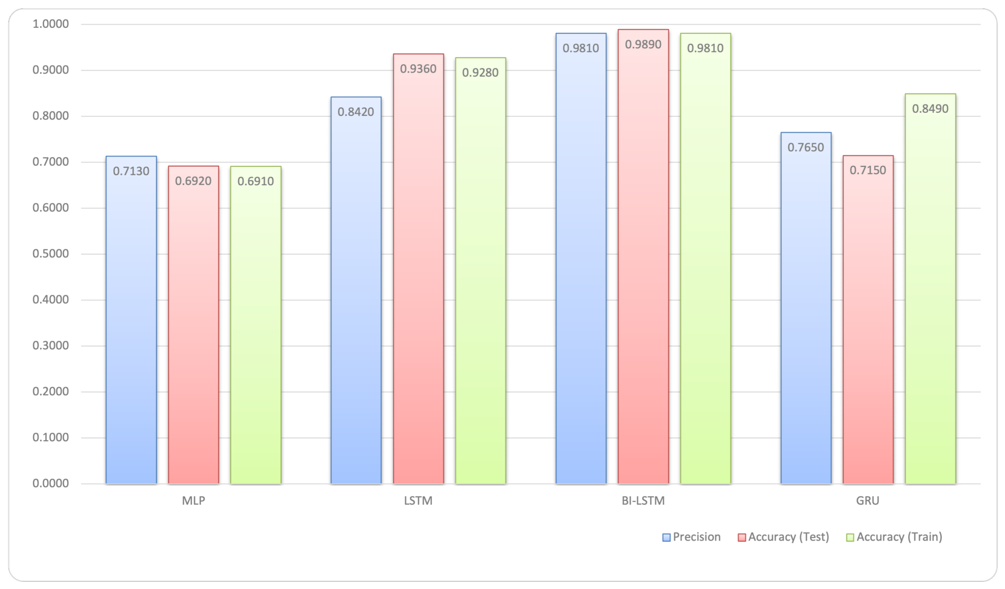
Figure 13.
Performance comparison of four neural network architectures (MLP, LSTM, Bi-LSTM, and GRU) on the DoW detection dataset after 20 training epochs. Three metrics are reported for each model: precision (blue), accuracy on test data (red), and accuracy on training data (green). The Bi-LSTM model achieves the highest values across all metrics, with a precision of 0.9810 and a test accuracy of 0.9850.
Figure 13.
Performance comparison of four neural network architectures (MLP, LSTM, Bi-LSTM, and GRU) on the DoW detection dataset after 20 training epochs. Three metrics are reported for each model: precision (blue), accuracy on test data (red), and accuracy on training data (green). The Bi-LSTM model achieves the highest values across all metrics, with a precision of 0.9810 and a test accuracy of 0.9850.
Table 1.
DDoS/DoW attack vectors.
Table 1.
DDoS/DoW attack vectors.
| Description | Potential Impact |
|---|
| Data injection in function events |
| Malicious data injected into function triggers, leading to unauthorized code execution [9]. | Malicious code execution, data theft, unauthorized resource access. |
| Broken authentication |
| Exploits authentication vulnerabilities to gain unauthorized access [10]. | Sensitive data access, data manipulation, account compromise. |
| Insecure deployment configuration |
| Exploits incorrect or vulnerable deployment configurations [11]. | Data access, manipulation, infrastructure compromise. |
| Functions with elevated privileges |
| Exploits functions with excessive permissions [12]. | Data leakage, infrastructure compromise, privilege escalation. |
| Inadequate control and recording |
| Exploits lack of visibility to carry out undetected malicious actions [13]. | Data loss, infrastructure compromise, privilege escalation. |
| Insecure third-party dependencies |
| Exploits vulnerabilities in third-party libraries [14]. | Data leakage, function compromise, privilege escalation. |
| Insecure storage of secrets |
| Access to insecurely stored API keys, passwords, and certificates [15]. | Account compromise, unauthorized infrastructure access. |
| Distributed denial of service (DDoS) |
| Multiple compromised systems generate malicious traffic [16]. | Service interruption, reputation damage. |
| Denial of wallet (DoW) |
| Exhausts funds via excessive requests in pay-per-use model [17]. | Increased costs, account suspension, service interruption. |
| Manipulating execution flow |
| Alters function execution sequence [18]. | Unauthorized function execution, data corruption, service interruption. |
| Inadequate exception handling |
| Exploits error handling weaknesses to reveal sensitive information [19]. | Data leakage, unauthorized access, vulnerability exploitation. |
Table 2.
Statistical methods for detecting DDoS/DoW attacks.
Table 2.
Statistical methods for detecting DDoS/DoW attacks.
| Algorithms Based on Distribution Models |
|---|
| The employment of such algorithms, including Poisson and Gaussian distribution models, facilitates the identification of variations in data flows, thereby establishing unusual thresholds that could signal the occurrence of attacks. This, in turn, enables the prompt detection and mitigation of threats [23]. |
| Algorithms based on time-series models |
| The employment of algorithms such as autoregressive integrated moving average (ARIMA) and hidden Markov models (HMMs) is attributable to their capacity to model and predict network traffic patterns. ARIMA employs historical data to predict future traffic values, facilitating the identification of deviations that may signal an attack. Hidden Markov models (HMMs) represent network traffic as a sequence of hidden states. Changes in the probabilities of these states can be indicative of anomalous activity [24]. |
| Algorithms based on the analysis of data randomness |
These are statistical methods that are utilized for the purpose of detecting anomalies in network traffic by measuring the randomness of data. A substantial increase in entropy is indicative of anomalous behavior as DDoS attacks characteristically result in elevated variability in network traffic [25].
Shannon entropy: Can be defined as the average amount of information contained in a dataset. In the context of DDoS (distributed denial of service) attacks, entropy can be calculated from the distribution of IP (Internet Protocol) addresses, ports, protocols, or traffic volumes. By observing the entropy for each type of event, high variations for each type of event could be flagged as possible DDoS/DoW attacks. Data flow-based entropy, also termed data flow entropy (DFE), is predicated on traffic characteristics [ 26]. Conditional entropy: This is a measure of the remaining uncertainty of a variable given knowledge of another variable. In the context of DDoS (distributed denial of service) attacks, conditional entropy can be utilized to analyze the relationship between different characteristics of network traffic [ 27]. Rényi entropy: This is a generalization of Shannon entropy that allows sensitivity to be adjusted to different probability levels. By varying a parameter, it is possible to assign greater or lesser weight to events according to their probability. In the context of DDoS (distributed denial of service) attacks, Rényi entropy can be utilized for the detection of attacks that do not cause drastic changes in Shannon entropy but do affect the distribution of less probable events [ 28].
|
Table 3.
Summary of key techniques and their contributions.
Table 3.
Summary of key techniques and their contributions.
| Classic Supervised Algorithms |
|---|
| A set of conventional machine learning (ML) methodologies are employed for the purpose of categorizing or labeling input data into predefined classes or categories. However, their threat detection capabilities are limited as they tend to be less effective at identifying complex non-linear patterns in large volumes of data and have a greater tendency to produce false positives [29,30,31]. |
| Decision Tree: Tree-based model that splits data into branches based on feature values, creating interpretable rules for classification. |
| Naïve Bayes: Probabilistic classifiers based on Bayes’ theorem assuming feature independence. |
| Random Forest: An ensemble machine learning approach that constructs multiple decision trees during training and outputs the mode of their predictions for classification tasks. Each tree is built from a random subset of data and features, reducing overfitting and improving generalization. Random forest is highly effective for detecting DDoS attacks due to its ability to handle high-dimensional data and identify complex patterns in network traffic with robust accuracy. |
| Gradient Boosting: An ensemble learning technique that builds multiple weak prediction models sequentially, where each new model corrects errors made by previous ones. It combines predictions through weighted voting to create a strong predictive model, particularly effective for classification and regression tasks in cybersecurity applications. Gradient boosting optimizes a loss function by iteratively adding models that follow the negative gradient, resulting in superior performance for anomaly detection in network infrastructure. |
| K-Nearest Neighbors (KNN): Instance-based learning that classifies data points based on the majority class of their k nearest neighbors in the feature space. |
| Neural Network (NN) |
| It is a type of artificial neural network architecture consisting of several layers of neurons, each connected to every neuron in the adjacent layers [32]. |
| Multilayer Perceptron (MLP): A type of neural network that has proven effective in a variety of classification problems, including the detection of DDoS attacks. It detects DDoS attacks in network infrastructure. |
| Deep Neural Network |
| A type of artificial neural network with multiple layers (RNN) between the input and output layers [33]. |
| LSTM (Long Short-Term Memory): Specialized RNN architecture with memory cells and gating mechanisms (input, forget, and output gates) that can learn long-term dependencies and avoid vanishing gradient problems, making them ideal for sequential data analysis in time-series attack detection. |
| BI-LSTM (Bidirectional LSTM): Processes sequences in both forward and backward directions simultaneously, capturing context from past and future states for improved pattern recognition in network traffic analysis. |
| GRU: A simplified variant of LSTM with fewer parameters, combining forget and input gates into a single update gate. GRUs are computationally efficient while maintaining the ability to capture long-term dependencies, making them suitable for real-time DDoS detection in resource-constrained IoT and fog computing environments. |
Table 4.
Advantages and disadvantages of statistical algorithms.
Table 4.
Advantages and disadvantages of statistical algorithms.
| Distribution-Based Algorithms |
|---|
| Advantages | Disadvantages |
|---|
| Conceptually simple and efficient. Good for detecting changes in overall volume or frequency. | They require a specific distribution to be assumed, which is unrealistic for complex data. They are sensitive to the accuracy of the estimated parameters (mean and variance). They may not capture complex relationships or temporal dependencies. |
| Time series-based algorithms |
| Advantages | Disadvantages |
| Capture temporary dependencies. Can predict future values. Good for detecting changes in patterns over time. | They can be computationally expensive (training; parameter tuning). They require a longer data history. They may assume stationarity or predictable patterns. |
| Randomness-based algorithms (entropy) |
| Advantages | Disadvantages |
| Sensitive to changes in transaction diversity. They can detect attacks that maintain normal volumes but change the composition (e.g., DDoS with varied but anomalous IPs; DoW with event variability and function calls). | Requires choosing the appropriate characteristics to calculate entropy. Needs to establish a threshold or normal range of entropy. Could fail if an attack perfectly mimics the normal distribution of characteristics (difficult). |
Table 5.
Summarizes the two scenarios in attack detection.
Table 5.
Summarizes the two scenarios in attack detection.
| Case | Interpretation |
|---|
| Low Entropy | Rare and predictable events. Normal behavior. No threat. |
| High Entropy | Many different events. Potential attack: entropy_potential_attack > ANOMALY_COUNT_THRESHOLD. |
Table 6.
The confusion matrix is influenced by the rates of false positives (FPs), true positives (TPs), false negatives (FNs), and true negatives (TNs) and ”bot” label to classified attacks. Green background is right classification.
Table 6.
The confusion matrix is influenced by the rates of false positives (FPs), true positives (TPs), false negatives (FNs), and true negatives (TNs) and ”bot” label to classified attacks. Green background is right classification.
| Observation/ Prediction | Positive | Negative |
|---|
| Positive | Attack traffic detected (bot = 1) and classified as attack correctly (TP). | Attack traffic detected (bot = 1) and classified as non-attack wrongly (FN). |
| Negative | Legitimate traffic (bot = 0) and classified as legitimate traffic wrongly (FP). | Legitimate traffic (bot = 0) and classified as legitimate traffic correctly (TN). |
Table 7.
Advantages and disadvantages of machine learning algorithms.
Table 7.
Advantages and disadvantages of machine learning algorithms.
| Decision Tree |
|---|
| Advantages | Disadvantages |
|---|
| Decision trees are easy to understand and interpret and can detect simple patterns in data. | Decision trees tend to be prone to overfitting, especially on large and complex datasets. |
| Random Forest |
| Advantages | Disadvantages |
| Random forest is an extension of decision trees that combines multiple trees to reduce overfitting. It can handle large and complex datasets, as well as irrelevant features. | Although it is more resistant to overfitting than a single decision tree, it may not be the best model for detecting highly sophisticated DoS or DoW attacks. |
| Gradient Boosting |
| Advantages | Disadvantages |
| Gradient boosting is a technique that allows for the analysis of more complex patterns in data. It can handle datasets that are not balanced. | It can be more complex to adjust and configure compared to decision trees and random forest. Compared to these, it may require more training time. |
| Naive Bayes |
| Advantages | Disadvantages |
| The naive Bayes algorithm is simple and computationally efficient. Furthermore, it can handle categorical and binary features, which is useful in detecting DDoS and DoW attacks, where features may be categorical in nature, such as traffic type or event types. Naive Bayes can also perform well even with relatively small datasets. | Due to the assumption of independence between features, naive Bayes is less capable of capturing complex relationships, which means that it may miss patterns in the data that other more advanced algorithms could detect. |
| KNN Classifier |
| Advantages | Disadvantages |
| It is simple to implement and understand. It does not require a complex training process as it stores training data and makes predictions based on the proximity of neighbors. It is effective for small- to medium-sized datasets. | Computationally more expensive with larger datasets as it requires calculating distances between all points. Its performance can be affected by irrelevant features or unequal scales between variables. Furthermore, the choice of the number of neighbors can significantly affect the results. |
Table 8.
Advantages and disadvantages of deep learning algorithms for detecting DDoS/DoW attacks.
Table 8.
Advantages and disadvantages of deep learning algorithms for detecting DDoS/DoW attacks.
| Multilayer Perceptron (MLP) |
|---|
| Advantages | Disadvantages |
|---|
| Easy implementation and training. Good performance on static data. | Does not handle time sequences. Ignores time dependencies in data. |
| Long Short-Term Memory (LSTM) |
| Advantages | Disadvantages |
| Handles long-term dependencies. Prevents gradient fading; ideal for complex temporal patterns. | Higher computational cost. More hyperparameters to adjust. |
| Bidirectional Long Short-Term Memory (Bi-LSTM) |
| Advantages | Disadvantages |
| Bidirectional context capture (past and future). Improved accuracy in detecting temporal anomalies. | Higher computational cost than LSTM. Complexity in implementation. |
| Gated Recurrent Unit (GRU) |
| Advantages | Disadvantages |
| Similar to LSTM but with fewer parameters. Resource-efficient. Good balance between performance and complexity. | It may be less accurate than LSTM in very long dependencies. |
Table 9.
Selection of 13 features of serverless events.
Table 9.
Selection of 13 features of serverless events.
| Execution & Timing Metrics |
|---|
| Function Trigger | Specific event source that initiated the function execution (HTTP request, a timer, a message queue trigger…). |
| Submit Time | Timestamp marking exactly when the function invocation request was submitted to the serverless platform. |
| Response Delay | The total duration from the moment the request was submitted until the response was received. |
| Invocation Delay | Latency between the request submission and the actual start of the function’s code execution. |
| ActiveFunctions: |
| ActiveFunctions | The total number of function instances that were running (active) within the application during the sampling period. |
| ActiveFunctions AtRequest | The count of concurrent function executions running at the exact moment the new request was received. |
| ActiveFunctions AtResponse | The count of concurrent function executions running at the moment the request was completed and the response was sent. |
| Resource Consumption (CPU) |
| maxcpu | The peak percentage of CPU utilization recorded during the function’s execution lifecycle. |
| avgcpu | The average (mean) percentage of CPU utilization throughout the duration of the function execution. |
| p95maxcpu | The 95th percentile of the maximum CPU usage. This is a statistical measure used to understand peak performance while excluding the most extreme 5% of outliers. |
| Infrastructure/Hardware Attributes |
| Vmcore countbucket | A categorical classification (bucket) indicating the number of CPU cores available on the underlying virtual machine (VM) that hosted the function instance. |
| Vmmemory bucket | A categorical classification (bucket) indicating the amount of RAM (memory) available on the underlying VM. |
| vmcategory | The category or tier of the underlying virtual machine (e.g., General Purpose, Compute Optimized, or Burstable) used to execute the workload. |
Table 10.
List of steps and processes required to train the model.
Table 10.
List of steps and processes required to train the model.
| Step | Process |
|---|
| 1 | Data Collection |
| | The first step is to collect a dataset containing examples of normal and malicious activities. This data must be labeled so that it is known when a threat occurs and when it does not. This labeled data is essential for training the supervised learning model. |
| 2 | Data Preprocessing |
| | The data must be cleaned and preprocessed to remove noise and ensure that it is in a format suitable for training. This may include data normalization and selection of relevant features. |
| 3 | Data Splitting |
| | The labeled dataset is divided into two parts: a training set and a test set. The training set is used to train the model, while the test set is used to evaluate its performance. |
| 4 | Learning & Modeling |
| | Model selection: A machine learning algorithm suitable for the cyber threat detection problem is chosen. Some common algorithms include decision trees, logistic regression, and naive Bayes. |
| | Model training: The labeled training set is used to train a supervised learning model to learn to distinguish between normal and malicious behavior based on the extracted features. |
| | Cross-validation and hyperparameter tuning: Cross-validation and hyperparameter tuning can be performed to optimize the performance of the model, ensuring that it is able to generalize correctly and avoid overfitting. |
| 5 | Model Evaluation |
| | Once the model has been trained, its performance is evaluated using the test suite. Metrics such as accuracy, completeness, F1-score and confusion matrix are calculated to measure the effectiveness of the model in detecting threats. The goal is to ensure that the model can effectively detect DoW threats without generating too many false positives. |
| 6 | Trained Model |
| | Tuning and optimization: If the model does not meet the desired performance requirements, adjustments can be made to the algorithm, feature selection or model parameters to improve the accuracy of the model. |
| | Real-time deployment: Once the model has been successfully trained and evaluated, it can be deployed in production as part of a real-time threat detection system. |
| | Continuous updating: Cyber threat detection is a constantly evolving field. Therefore, it is important to update and maintain the model as new threats emerge and data changes over time. |
Table 11.
Layers of the MLP neural network and parameters in each layer.
Table 11.
Layers of the MLP neural network and parameters in each layer.
| Layer | Inputs | Layer 1 | Layer 2 | Layer 3 | Output |
|---|
 |
| Input Shape | 13 | 13→64 | 64→32 | 32→1 | – |
| Output Shape | – | 64 | 32 | 1 | 1 |
| # Param | – | 896 | 2080 | 33 | 2011 |
| Layer 1 (Hidden 1) |
| Input with 13 features to a dense layer with 64 neurons (13→64). |
| Layer 2 (Hidden 2) |
| Reduces dimensionality from 64 to 32 neurons (64→32). |
| Layer 3 (Hidden 3) |
| Dense layer that generates a single characteristic prior to output (32→1). |
| Output |
| Final neuron with logistic activation (sigmoid) (1→1). |
Table 12.
Layers of the LSTM neural network and parameters in each layer.
Table 12.
Layers of the LSTM neural network and parameters in each layer.
| Layer | Inputs | Layer 1 | Layer 2 | Layer 3 | Layer 4 | Output |
|---|
 |
| Input Shape | None, 13, 1 | N, 13, 64 | None, 64 | None, 64 | None, 1 | |
| Output Shape | | None, 13, 64 | None, 64 | None, 64 | None, 1 | 1 |
| # Param | | 16,896 | 33,024 | 4160 | 65 | 54,145 |
| Inputs: None, 13, 1 |
| Input tensor with time sequences of length 13 and a single variable. |
| Layer 1 (LSTM_2) |
| Processes the sequence step by step and returns the complete sequence. |
| Layer 2 (LSTM_3) |
| Compresses temporal information, returning only the last hidden state. |
| Layer 3 (Dense_2) |
| Dense layer with ReLU activation to refine extracted patterns. |
| Layer 4 (Dense_3) |
| Sigmoid activation for final prediction. |
Table 13.
Layers of Bi-LSTM neural network and parameters in each layer.
Table 13.
Layers of Bi-LSTM neural network and parameters in each layer.
| Layer | Inputs | BI-LSTM 1 | BI-LSTM 2 | Dense | Output |
|---|
 |
| Input Shape | None, 13, 1 | None, 13, 128 | None, 128 | None, 1 | |
| Output Shape | | None, 13, 128 | None, 128 | None, 1 | 1 |
| # Param | | 33,792 | 98,816 | 129 | 132,737 |
| Input |
| 13-step sequence, 1 feature. |
| Layer 1 (Bi-LSTM 1) |
| 64 units per direction, returns the complete sequence. |
| Layer 2 (Bi-LSTM 2) |
| 64 units per direction, returns last step. |
| Layer 3 (Dense) |
| Full connection, sigmoid activation. |
| Output |
| Shape (None, 1) |
Table 14.
Layers of the GRU-based neural network and parameters in each layer.
Table 14.
Layers of the GRU-based neural network and parameters in each layer.
| Layer | Inputs | GRU | Dropout | Dense 1 | Output |
|---|
 |
| Input Shape | None, 13, 1 | None, 13, 1 | None, 64 | None, 64 | |
| Output Shape | | None, 64 | None, 64 | None, 1 | 1 |
| # Param | | 12,864 | 0 | 650 | 13,525 |
| Layer 1 (GRU) |
| Processes the input time sequence and returns a feature vector (last hidden state). |
| Layer 2 (Dropout) |
| Dropout rate of 0.5 (50%), randomly deactivates neurons to prevent overfitting. |
| Layer 3 (Dense 1) |
| Fully connected layer with 10 neurons for intermediate processing. |
| Layer 4 (Dense 2/Output) |
| Single neuron with sigmoid activation function for binary classification. |
Table 15.
Performance comparison of statistical, machine learning, and deep learning methods.
Table 15.
Performance comparison of statistical, machine learning, and deep learning methods.
| Algorithm | Precision | Accuracy | FPR | FNR | Trans. Time (s) | Comp. Cost | Latency |
|---|
| Entropy | 0.8308 | 0.8308 | 0.000 | 0.004 | 7.77 × 10⁻⁵ | Very Low | Very Low |
| Decision Tree | 0.9348 | 0.7399 | 0.045 | 0.352 | 2.80 × 10⁻⁴ | Very Low | Low |
| Random Forest | 0.7921 | 0.6484 | 0.147 | 0.439 | 2.63 × 10⁻⁴ | Low | Low |
| Gradient Boost | 0.9006 | 0.8656 | 0.094 | 0.152 | 2.73 × 10⁻⁴ | Med. | Med. |
| Naive Bayes | 0.7018 | 0.6347 | 0.248 | 0.415 | 2.20 × 10⁻⁴ | Very Low | Very Low |
| KNN | 0.9565 | 0.6371 | 0.022 | 0.509 | 5.10 × 10⁻⁴ | Med. | Med. |
| MLP | 0.7130 | 0.6920 | 0.272 | 0.323 | 2.58 × 10⁻⁴ | Low | Low |
| LSTM | 0.8420 | 0.9360 | 0.185 | 0.012 | 1.36 × 10⁻³ | High | High |
| BI-LSTM | 0.9810 | 0.9850 | 0.019 | 0.013 | 1.35 × 10⁻³ | Very High | Very High |
| GRU | 0.7650 | 0.7150 | 0.210 | 0.317 | 9.66 × 10⁻⁴ | High (lower than LSTM) | Med. |




 ,
,