Fractional Epidemic Modeling: Theoretical Constructions and Estimation Strategies

Abstract

This paper presents a generalized epidemic modeling framework based on g-tempered Caputo fractional derivatives with discrete time delays. The proposed approach incorporates nonlocal memory effects, nonlinear temporal scaling, and delayed epidemiological responses within a unified mathematical structure. The introduction of the nonlinear time transformation $g\left(t\right)$ and the tempering parameter $\lambda$ eliminates the unrealistic infinite-memory behavior associated with classical power-law kernels while simultaneously introducing new challenges related to parameter identifiability and inverse problems. We investigate the structural properties of the resulting dynamical systems and show that the associated inverse problem is inherently ill-posed. To illustrate the practical implications of these results, the framework is applied to a delayed SIQR epidemiological model. Numerical simulations are performed using a generalized L1-type scheme adapted to delayed fractional histories, and a multi-phase parameter estimation procedure is proposed to address the ill-posedness of the reconstruction problem. The results demonstrate the ability of the model to capture both short- and long-term memory effects in epidemic evolution while highlighting the challenges of statistical identifiability in generalized fractional systems.

1. Introduction

Data describing the progression of diseases can be analyzed for multiple purposes, including prediction and policy evaluation. The primary objective of this paper is to develop a flexible and broadly applicable model of epidemic dynamics. The proposed framework is designed to accommodate different diseases, healthcare systems, and spatial scales, while remaining consistent with observed data. This consistency enables prediction of subsequent epidemic waves and numerical simulation of intervention strategies such as vaccination and quarantine.

Modeling epidemic progression is inherently challenging. The model should capture key features such as the timing and magnitude of the outbreak peak, the transient dynamics leading to that peak, and the temporal distribution of cases. It should also account for the immediate effects of interventions. To achieve this, the model incorporates a memory mechanism that reflects both long-term cumulative effects and short-term impulsive actions ([1,2,3]). Although these aspects have been studied individually, they are rarely integrated within a single framework; here, we address this gap. The resulting model supports statistical analysis for estimating disease-specific parameters.

Since the system dynamics are governed by derivatives, we extend standard first-order models in two directions. First, we introduce g-tempered fractional derivatives ([4,5]) to represent time-scale variability through a function g. This formulation allows the identification of parameters associated with impulsive events, including discontinuities in the solution ([6]).

Second, we incorporate fractional-order derivatives to provide additional flexibility in capturing complex dynamics ([1,7,8]). While fractional calculus is well established, not all definitions yield meaningful improvements in modeling. Selecting an appropriate derivative is therefore critical and constitutes a key contribution of this paper ([5,9]). For a broader discussion on modeling real-world phenomena using fractional calculus, see [10]. We propose a unified model combining these two extensions, enabling the simulation of a wide range of epidemic scenarios.

In classical epidemic models, memory effects are often incorporated using delay differential equations (see, e.g., [11,12,13,14]). Such models can reproduce phenomena like oscillatory behavior. However, a single discrete delay is limited, as it depends only on the system state at a specific past time $t-\tau$ and does not reflect the cumulative influence of prior dynamics.

A more general approach is provided by distributed or state-dependent delay models, in which the system history is represented through functional dependence on the trajectory $x_t$ [15]. These formulations allow for time-varying and state-dependent delays, including responses based on aggregated past behavior. Nevertheless, they still rely on representations of past states rather than on the evolution process itself.

To capture both the magnitude and temporal structure of memory effects, we employ fractional-order derivatives. These operators introduce nonlocal memory directly into the governing equations, enabling the modeling of long-range temporal dependence [9,16]. In this context, the choice of fractional operator and its parameters is critical, as it determines the effective memory, time-scale properties, and qualitative behavior of the solutions.

An additional objective of this paper is to develop models that are both flexible and computationally tractable for predictive analysis. This requires appropriate analytical and numerical methods adapted to the structure of the generalized fractional operators. In particular, standard techniques such as the step method may not be suitable. The analysis of such operators motivates the proposed framework and supports further methodological development.

The primary objective of the proposed framework is to introduce additional parameters that improve the ability of epidemiological models to fit real-world data. These parameters must be calibrated for each disease; however, identifying those that control the qualitative behavior of the system can simplify analysis and support prediction of future epidemic waves. This underscores the importance of statistical inference for reliable parameter estimation.

The proposed extensions are not tied to a specific model and can be incorporated into a broad class of epidemiological frameworks. For clarity, we illustrate them using representative examples. This paper constitutes the first stage of a broader research program, focusing on model formulation and initial analysis; detailed stability studies and data-driven calibration are deferred to future work.

The development of a general epidemiological model with memory effects can be organized into three stages. The first stage, addressed in this paper, concerns model formulation and the selection of operators governing the dynamics. In particular, we introduce generalized fractional derivatives with parameters describing temporal memory and establish well-posedness of the forward problem, enabling numerical implementation.

The second stage involves the development of numerical methods adapted to these generalized operators. The presence of fractional, tempered, and g-dependent structures introduces challenges that are not adequately handled by standard schemes. We therefore present preliminary simulations to illustrate the model behavior and to support initial fitting to data. This step is essential because the associated inverse problem—parameter estimation from observed trajectories—is ill-posed and cannot be resolved analytically.

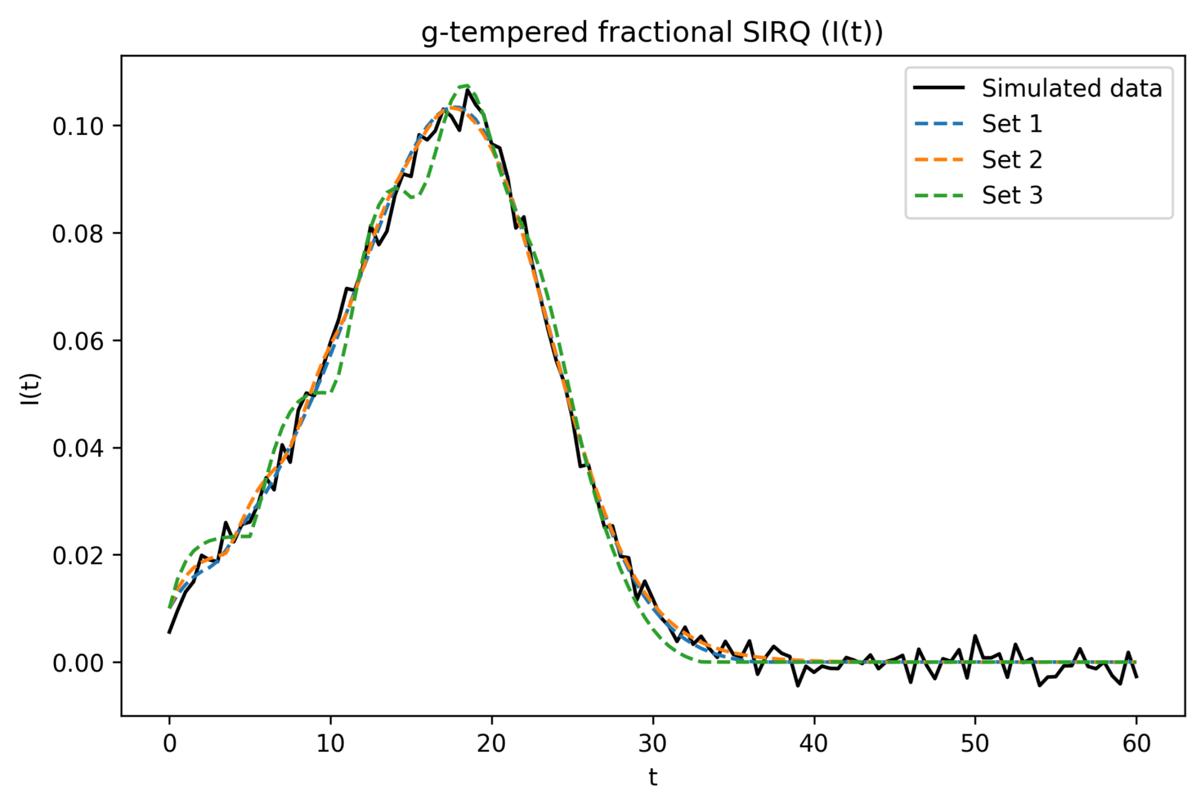
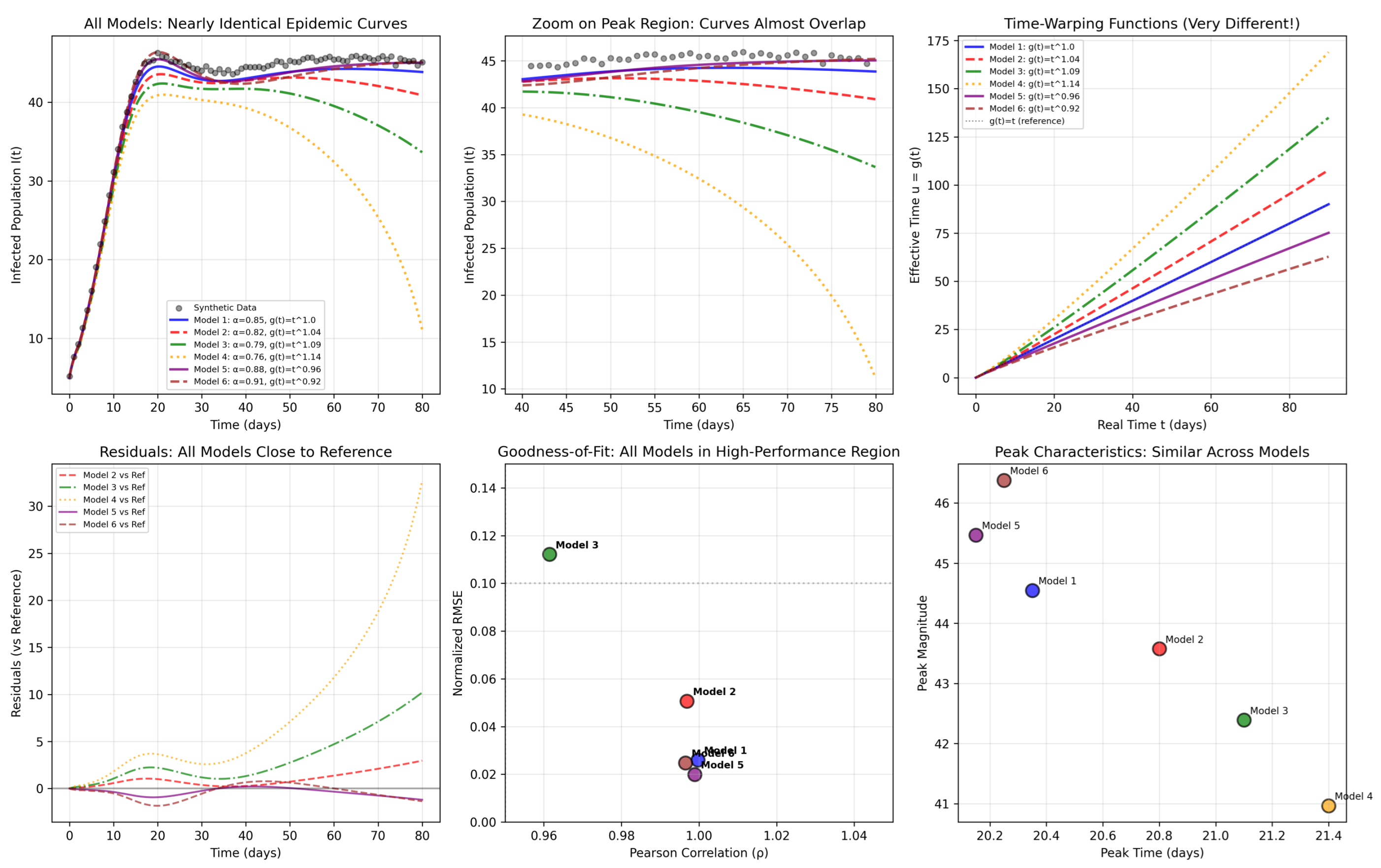
The third stage concerns statistical calibration using epidemiological data. Existing approaches for fractional models (see, e.g., [17,18]) may be extended to this setting, although the increased number of parameters substantially complicates the inverse problem. In particular, different parameter sets may produce similar epidemic trajectories, raising issues of identifiability, especially for parameters related to memory and time transformation.

The integration of mathematical analysis, numerical methods, and statistical inference is therefore essential for practical applications. While this paper establishes the foundation for such an approach, the development of robust data-driven calibration procedures remains an open problem.

For further context, we refer to selected studies illustrating the application of mathematical and statistical methods in epidemiological modeling. Foundational material is presented in ([19] Chapter 8) and [20], while multi-stage modeling approaches are discussed in [21,22]. Classical compartmental models are reviewed in [23] (see Chapter 12 for results related to the present paper, based on SIR models with ordinary derivatives). Fractional-order models using Caputo derivatives are analyzed in [24]; compared with the framework proposed here, these models involve fewer parameters and do not include delay effects. The role of mathematical modeling in public health evaluation is further emphasized in [25]. Most existing statistical studies focus on estimating constant transmission parameters. In contrast, the present work extends this perspective by introducing parameters that describe memory effects and temporal variability. To the best of our knowledge, even in fractional models based on Caputo derivatives (i.e., with a single parameter $\alpha$), statistical calibration has been limited, with most results relying on numerical simulations. Extending inference procedures to include such effects remains an important direction when epidemiological data are available.

Finally, while simplified models with fewer parameters are often easier to analyze, they may fail to capture essential features of the dynamics, as discussed in [26].

2. Construction of Mathematical Models

It is important to emphasize that the general model proposed in this paper does not modify the fundamental properties of established nonlinear epidemiological models, such as the SIR, SIQR or SEIR frameworks. These models are well justified, and their parameters have been extensively studied through statistical analysis. Instead, the proposed formulation extends these models by incorporating additional mechanisms that account for memory effects. In its abstract form, given by (8) and (9), the model introduces a unified structure for controlling both local and global memory. This includes mechanisms responsible for deviations that may lead to oscillatory behavior and other qualitative features of the solutions (see [27]), as well as nonlocal effects represented by fractional-order derivatives. It can be expressed in differential form as follows:

$$\mathcal{D}x\left(t\right)=F(t,x(t),x_t)$$

for $t\in [0,T]$ and

$$x\left(t\right)=\varphi \left(t\right)\mathrm{for}t\in [-\tau ,0],$$

where $\mathcal{D}$ is a multi-parameter dependent derivative and F is a vector-valued right-hand side that describes the model with the set of parameters currently under consideration. The function x belong to the appropriate space of solutions X which also describe the expected regularity of solutions. We will assume that $D:X\to X$. Since the right-hand side is typically n-dimensional ($n=4$ in the SIQR model), we will assume that $X={\left(C\right(-\tau ,T\left]\right)}^4$. Hovewer, spaces of discontinuous functions can be also useful, as described in [6]. The sets of parameters for $\mathcal{D}$ will be described when this operator will be chosen.

Our focus on the left-hand side of the equation system, its parameters, and their impact on the dynamics of changes in the solutions. We select only those parameters of the derivative that affect the ability to model the course of the epidemic.

To simplify the discussion and avoid any historical oversights, we will start by reviewing the most important models and focusing on the simplest memory effect, the delay effect. Although these models were developed to incorporate the oscillatory nature of the phenomenon into their solutions, our discussion will focus solely on the memory effect.

Therefore, we should propose a flexible model that takes into account all the effects of memory and can be applied to different epidemics. This model should include a suitable set of parameters that enable numerical simulations based on new algorithms. It should also allow for verification using statistical analysis methods. The model should build on current models by considering dynamic effects (derivative parameters) as well as static ones (biological factors on the right-hand side of the equation). However, we would like to point out that having too many parameters creates selection problems and generally leads to an ill-posed problem. The solution is to conduct simulations that allow us to match solutions to real data, and then verify such hypotheses using statistical methods. We have already selected the set of parameters to be controlled through derivatives in the model, and we will now demonstrate how to construct it.

2.1. Some of the Considered Models

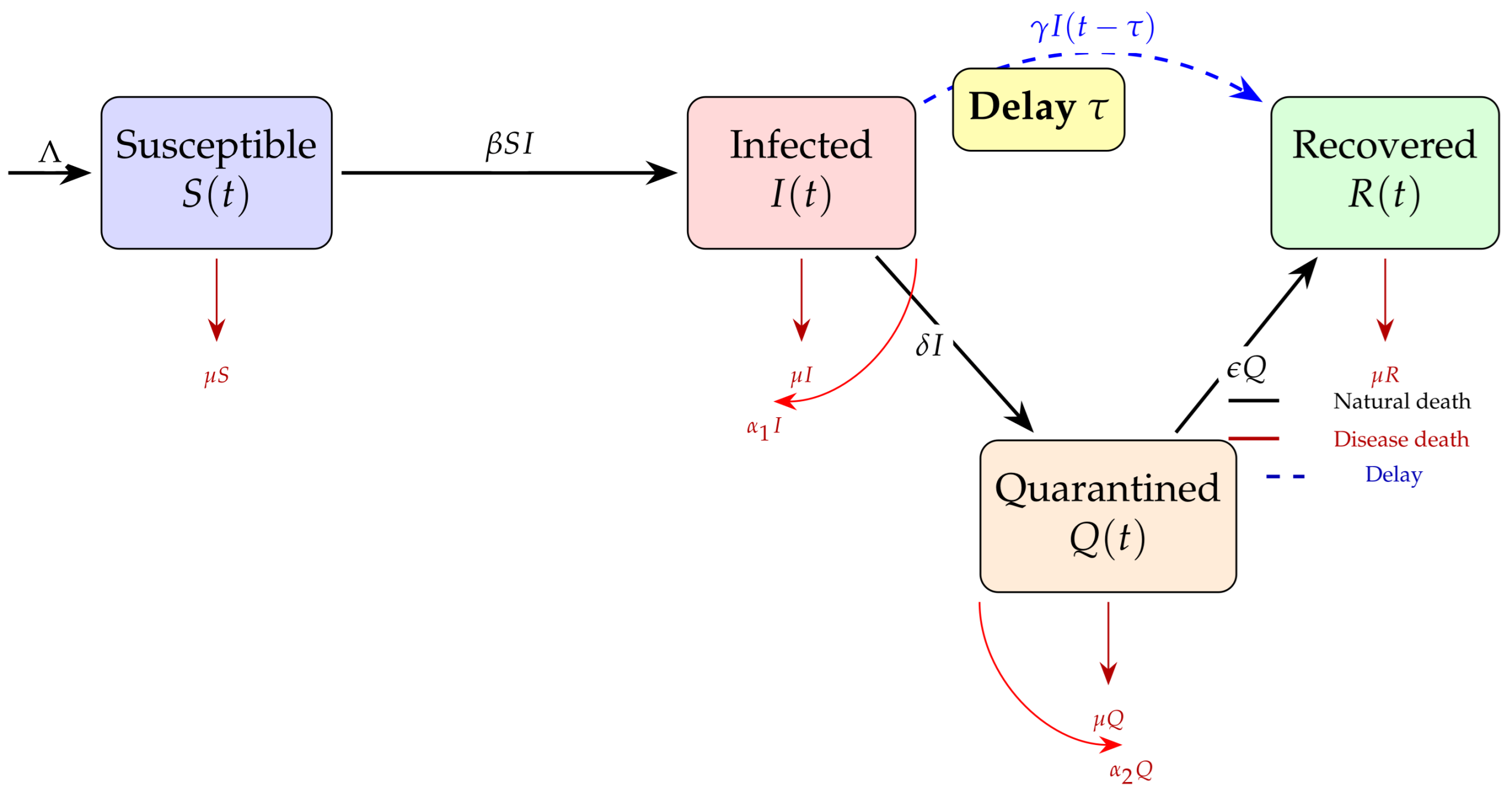
The following SIQR epidemic model with a single delay is considered in [28] (cf. also [29]):

$$\left\{\begin{array}{c}{S}^{\prime }=\Lambda -\beta SI-{\mu }_{0}S,\hfill \\ I^{\prime }=\beta SI-{\alpha }_{1}I-\gamma I(t-\tau )-\sigma I-{\mu }_{0}I,\hfill \\ Q^{\prime }=\sigma I-\theta Q-{\alpha }_{2}Q-{\mu }_{0}Q,\hfill \\ R^{\prime }=\gamma I(t-\tau )+\theta Q-{\mu }_{0}R,\hfill \end{array}\right.$$

(1)

where $\Lambda$, ${\mu }_0$, $\beta$, $\sigma$, $\gamma$, $ϵ$, ${\alpha }_1$, ${\alpha }_2$ are parameters whose notation is consistent with epidemiological models, and which will be reviewed in

Table 1. Biological parameters and their epidemiological definitions.

Parameter	Definition	Biological/Epidemiological Significance
$\Lambda$	Recruitment rate	Constant inflow of new individuals into the susceptible (S) class via birth or migration.
$\beta$	Transmission rate	Force of infection representing the probability of successful transmission per contact between S and I.
$\eta$	Interaction rate	Rate of temporary immunity loss or breakthrough re-infection due to interaction between R and I classes.
${\mu }_0$	Natural death rate	Baseline non-disease mortality rate applied uniformly across all compartments.
$\sigma$	Quarantine rate	Rate of public health screening, detection, and subsequent isolation of infectious individuals.
$\theta$	Recovery rate	Clinical clearance or discharge rate of individuals transitioning from quarantine to the recovered state.

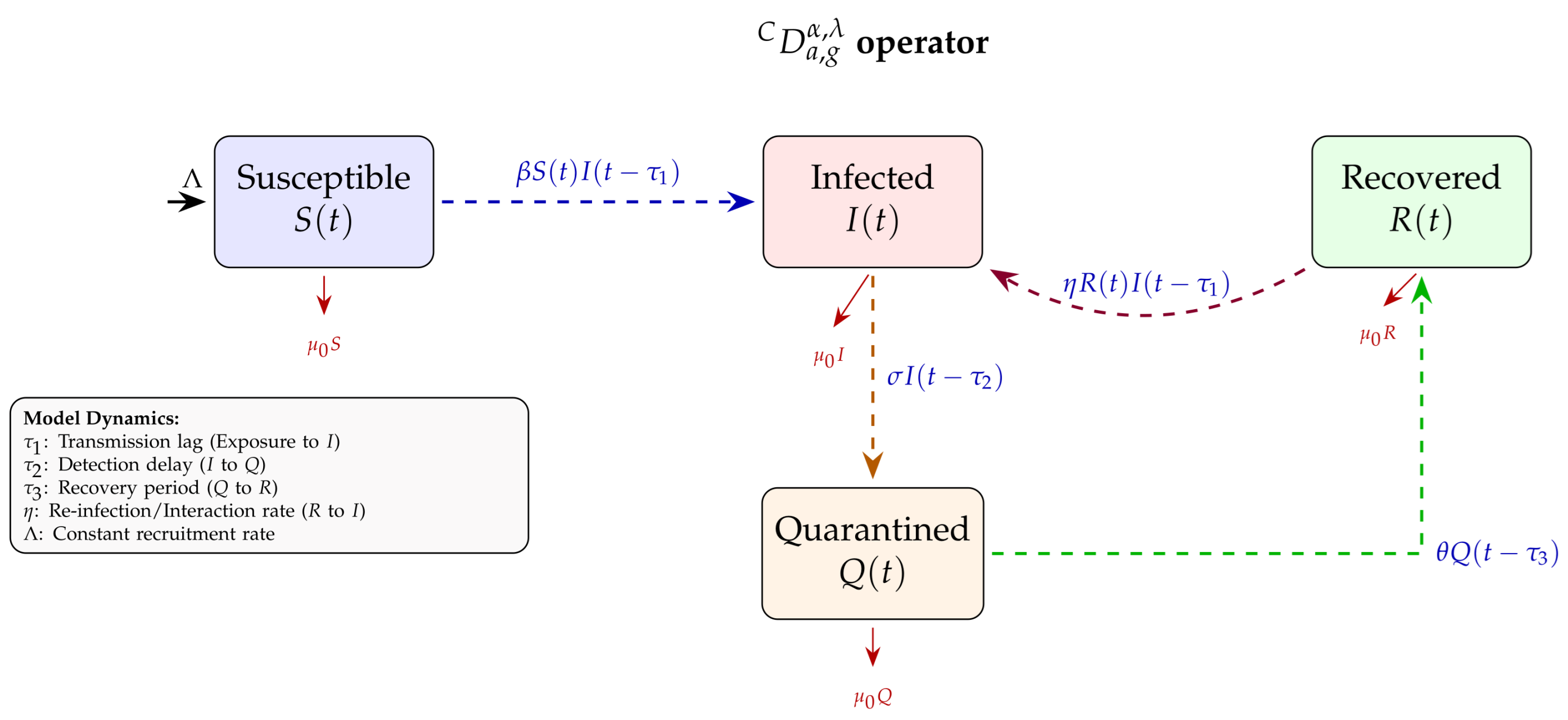
when discussing the generalized multi-delayed model; S, I, Q, R are control variables and $\tau$ is the time-delay (Figure 1). In model (1), the parameters $\theta$ and ${\alpha }_2$ both represent linear exit rates from the quarantine compartment Q, but they distinguish distinct epidemiological destinations: $\theta$ denotes the rate of safe recovery into compartment R, whereas ${\alpha }_2$ isolates the disease-induced mortality rate of quarantined individuals. For consistency of exposition ([28]), we employ the same baseline notation for demographic, transmission, and transition rates in both frameworks, noting that model (7) introduces an updated multi-delay structure (${\tau }_1,{\tau }_2,{\tau }_3$) and an immunity-loss parameter ($\eta$). Although this is not specified in [28], the numerical simulations in this paper are performed when $I\left(t\right)$ is constant for $t\in [-\tau ,0]$. In general, however, any continuous initial function, $T\left(t\right)={\varphi }_I\left(t\right)$, can be chosen for $t\in [-\tau ,0]$.

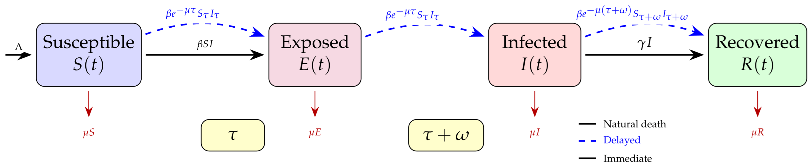
The delayed SEIR model (Figure 2) is considered in the following form:

$$\left\{\begin{array}{c}{\displaystyle \frac{dS}{dt}}=\Lambda -\beta S(t)I(t)-{\mu }_{0}S(t),\hfill \\ {\displaystyle \frac{dE}{dt}}=\beta S(t)I(t)-\beta e^{-{\mu }_0\tau }S(t-\tau )I(t-\tau )-{\mu }_{0}E(t),\hfill \\ {\displaystyle \frac{dI}{dt}}=\beta e^{-{\mu }_0\tau }S(t-\tau )I(t-\tau )-\beta e^{-{\mu }_0(\tau +\omega )}S(t-\tau -\omega )I(t-\tau -\omega )-{\mu }_{0}I(t),\hfill \\ {\displaystyle \frac{dR}{dt}}=\beta e^{-{\mu }_0(\tau +\omega )}S(t-\tau -\omega )I(t-\tau -\omega )-{\mu }_{0}R(t).\hfill \end{array}\right.$$

Note that in the above model, the demographic notation remains consistent ($\Lambda ,{\mu }_0,\beta$), but the compartmental structure shifts to track an Exposed population (E). Here, the delay $\tau$ shifts meaning to represent the fixed incubation duration, while $\omega$ represents the active infectious window prior to natural recovery, with both phases attenuated by the natural survival factors $e^{-{\mu }_0\tau }$ and $e^{-{\mu }_0(\tau +\omega )}$ respectively.

For this model, the initial functions for I and S had to be determined. Specifically, $I\left(t\right)={\varphi }_I\left(t\right)$ for $t\in [-\tau -\omega ,0]$, and $S\left(t\right)={\varphi }_S\left(t\right)$ for $t\in [-\tau ,0]$. Note that it is usually formally defined on $[-\tau -\omega ,0]$).

2.2. Basic Fractional Models

The usefulness, or rather, the necessity, of using fractional derivatives in epidemiological models has long been demonstrated. An interesting overview of the development of such models and their use of fractional derivatives in them can be found, for example, in ([8], Section 3.2).

Fractional-order calculus has emerged as a powerful modeling framework for complex dynamical systems, particularly those exhibiting memory and hereditary properties. To demonstrate its applicability effectively, it is essential to select fractional derivatives that significantly influence the behavior of the model in question ([11,27]). This enables a deeper analysis of solution properties and often leads to more accurate representations of real-world phenomena (cf. [12,30,31]).

Recent studies (cf. [9,32]) suggest that fractional derivatives are particularly well-suited for modeling epidemic dynamics, as they inherently incorporate memory effects and capture universal characteristics that are often overlooked in classical integer-order formulations. In this paper, we consider models of the general form

$$\mathcal{D}x\left(t\right)=f\left(t,x\left(t\right),x(t-\tau )\right),x\left(s\right)=\psi \left(s\right)\mathrm{for}s\in [-\tau ,0],$$

where $t\in [0,T]$ and $\mathcal{D}$ denotes a fractional differential operator (see also [33]). To focus the attention of the reader on epidemiological models, the cases of function f considered in this paper will always ensure that the solutions are bounded and positive for positive initial values at $t=0$ and that the superposition operator $N_f$, generated by f, takes values in phase space X, i.e., when $\psi$ belongs to X (see Section 5 for more details).

Fractional-order operators are characterized by their intrinsic non-locality, meaning that the evolution of the system at a given time depends on its entire past history rather than only its current state. This property distinguishes fractional models fundamentally from classical integer-order formulations. As a result, the associated solution operators incorporate memory effects directly into the dynamics, leading to a modified temporal structure in which past states continuously influence present evolution. One of the related models is the SIQR model, which is relevant to Coronavirus research due to its focus on people in quarantine (cf. [28,34]). It is important to note that the model should take the effect of delays into account and be based on differential equations with delay (see [32,35,36,37]).

2.3. Fractional Calculus

The following general class of operators, introduced in [4], will prove particularly useful when considering mathematical models in epidemiology:

Definition 1

([4,5]). Let $g\in C^1\left([a,b]\right)$ be a positive increasing function such that $g^{\prime }\left(t\right)\ne 0$, for all $t\in (a,b)$.

The generalized fractional (or briefly g-fractional) integral of a function $x:[a,b]\to E$ of order $\alpha >0$ and parameter $\lambda \in {\mathbb{R}}^{+}$ is that defined by

$$I_{a,g}^{\alpha ,\lambda }x(t)={\displaystyle \frac{1}{\Gamma (\alpha )}}{\int }_a^t{\left(g(t)-g(s)\right)}^{\alpha -1}{e}^{-\lambda \left(g(t)-g(s)\right)}x(s)g^{\prime }(s)ds,$$

(2)

where $-\infty \le a<b\le \infty$. For completeness, we define $I_{a,g}^{\alpha ,\lambda }x(a)=0$.

The parameter $\lambda \ge 0$ is the ‘tempering’ parameter. The exponential term $e^{-\lambda \left(g\right(x)-g(t\left)\right)}$ is the key modification that distinguishes this from a standard g-fractional integral.

Let

$$A{C}_g^n([a,b])=\left\{f:{\left({\displaystyle \frac{d}{dg}}\right)}^{k}f\in AC([a,b]),k=0,\dots ,n-1\right\}$$

be the subspace of the space of absolutely continuous functions $AC\left(\right[a,b\left]\right)$.

The Caputo g-tempered fractional derivative is then defined as the inverse of this integral operator ([38]). For $n-1<\alpha <n$ (where n is an integer for $0<\alpha <1$), the definition is as follows:

$$\begin{array}{ccc}\hfill \left({}^C\mathcal{D}_{a,g}^{\alpha ,\lambda }f\right)(x)& =& I_{a,g}^{n-\alpha ,\lambda }{\left({\displaystyle \frac{d}{dg\left(x\right)}}\right)}^{n}f(x)\hfill \\ & =& {\displaystyle \frac{1}{\Gamma (n-\alpha )}}{\int }_a^x{\left(g\right(x)-g(t\left)\right)}^{n-\alpha -1}{e}^{-\lambda \left(g\right(x)-g(t\left)\right)}{f}_g^{\left(n\right)}(t)dg(t),\hfill \end{array}$$

(3)

where $f_g^{\left(n\right)}(t)={\left({\displaystyle \frac{d}{dg\left(t\right)}}\right)}^{n}f(t)$.

Under the assumptions $f\in A{C}_g^n\left([a,b]\right)$, the following inverse relations hold. Left-inverse formula. If $f\in A{C}_g^n\left([a,b]\right)$, then

$$I_{a,g}^{\alpha ,\lambda }\left({}^C\mathcal{D}_{a,g}^{\alpha ,\lambda }f\right)(x)=f(x)-e^{-\lambda (g(x)-g(a))}{\displaystyle \sum _{k=0}^{n-1}}{\displaystyle \frac{{(g(x)-g(a))}^k}{k!}}{f}_g^{\left[k\right]}(a).$$

In our case, when $0<\alpha <1$, the definition of this derivative simplifies to

$$\left({}^C\mathcal{D}_{a,g}^{\alpha ,\lambda }f\right)(x)={\displaystyle \frac{1}{\Gamma (1-\alpha )}}{\int }_a^x{(g(x)-g(t))}^{-\alpha }{e}^{-\lambda (g(x)-g(t))}\left({\displaystyle \frac{d}{dg(t)}}f(t)\right)dg(t).$$

(4)

Therefore,

$$I_{a,g}^{\alpha ,\lambda }\left({}^C\mathcal{D}_{a,g}^{\alpha ,\lambda }f\right)(x)=f(x)-e^{-\lambda (g(x)-g(a))}f(a).$$

(5)

Right-inverse formula. If $f\in L^1([a,b],dg)$, then

$${}^C\mathcal{D}_{a,g}^{\alpha ,\lambda }\left(I_{a,g}^{\alpha ,\lambda }f\right)\left(x\right)=f(x).$$

(6)

Thus, the g-tempered Caputo derivative is the right inverse of the corresponding g-tempered fractional integral on $L^1([a,b],dg)$, while the integral operator acts as a left inverse modulo generalized initial terms. It is worthwhile studying the reciprocals of integral and differential operators in Hölder spaces, given the properties of epidemiological models. This is especially true when the right-hand side of the system of equations contains continuous functions. Those interested will find relevant results in [38] (in particular, Theorem 5).

This generalizes the other known cases: for $\lambda =0$ it is the Caputo g-fractional derivative, in the case $g\left(t\right)=t$ it is the Caputo tempered derivative. If both assumptions are satisfied, we obtain the classical Caputo derivative. The g-tempered fractional calculus has important applications in modeling physical or biological phenomena in which a system exhibits both power-law scaling (due to the fractional order) and exponential tempering that truncates heavy tails. This type of fractional calculus is known as ‘g-fractional calculus’ or ‘$\psi$-fractional calculus’ (although the function $\psi$ has a different meaning in this paper). The corresponding integrals and derivatives are referred to as ‘g-fractional integrals’ or ‘fractional integrals with respect to a function’ (also known as ‘$\psi$-fractional integrals’) (see, for example, [5]). 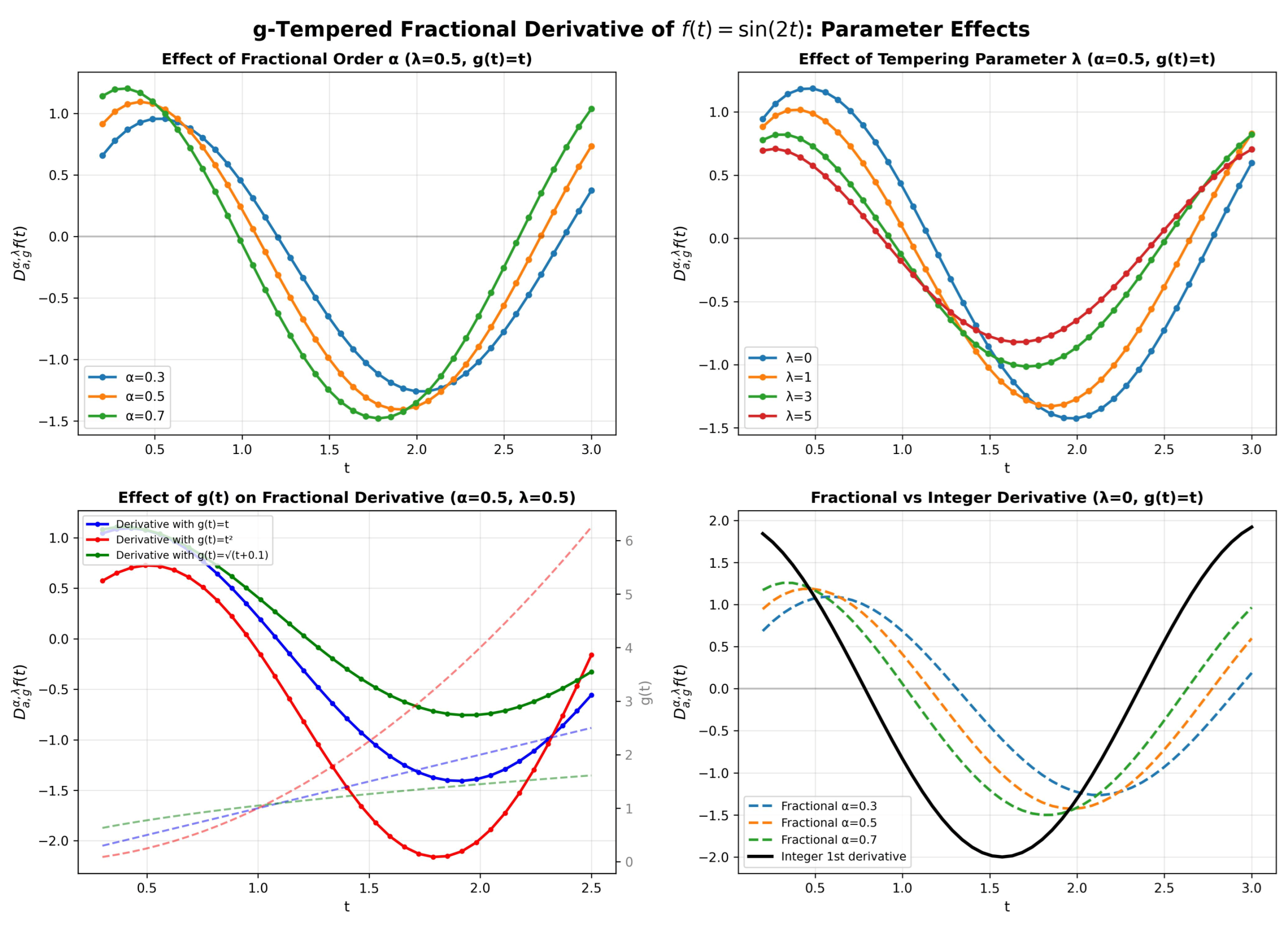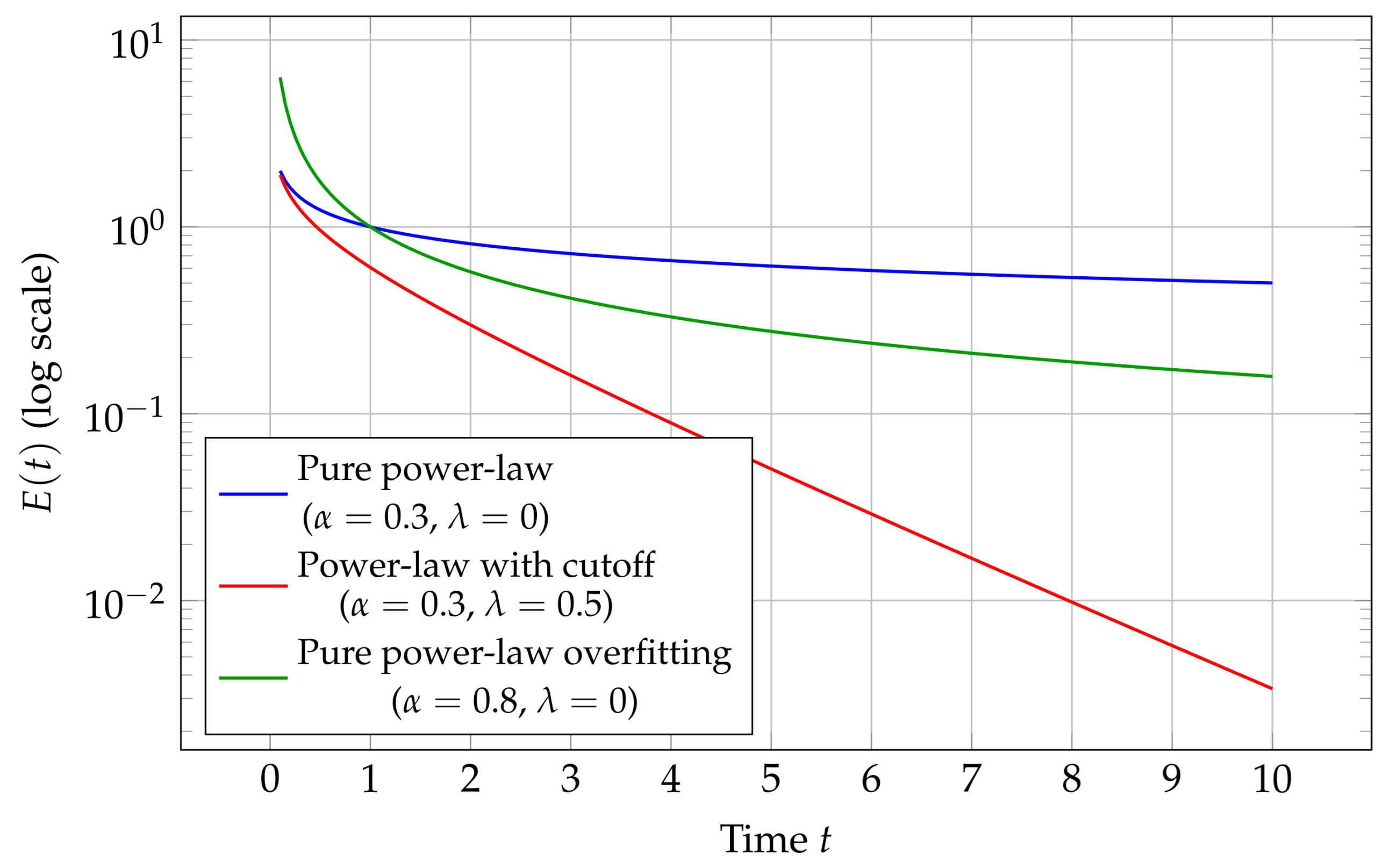Figure 3 shows the main properties of the parameters. Note, that the fractional integral operators considered here are particular cases of generalized fractional integrals with Sonine-type kernels (see, for example, ([39])).

There are many different types of fractional derivative (see, for example, [5,40,41,42]). Due to the memory effect, we are only interested in non-local epidemiological models. The most useful derivative of a fractional-order equation is the Caputo derivative due to its ability to naturally account for initial conditions (see [40] for a discussion of the Riemann-Liouville derivative and initial conditions for differential equations). The Caputo derivative possesses two features that allow it to be applied to the models under consideration: non-locality to provide a memory effect, and control of the dynamics. However, in this paper, we will also highlight certain extensions with a greater number of parameters that can be fitted to epidemiological data to ensure consistency between the model’s results and the data. We will discuss this issue in the next section.

2.4. New Model

To fix our attention, let us consider the following general SIQR model:

$$\left\{\begin{array}{c}{}^C\mathcal{D}_{a,g}^{\alpha ,\lambda }S(t)=\Lambda -\beta S(t)I(t-{\tau }_1)-{\mu }_{0}S(t)\hfill \\ {}^C\mathcal{D}_{a,g}^{\alpha ,\lambda }I(t)=\beta S(t)I(t-{\tau }_1)+\eta R(t)I(t-{\tau }_1)-\sigma I(t-{\tau }_2)-{\mu }_{0}I(t)\hfill \\ {}^C\mathcal{D}_{a,g}^{\alpha ,\lambda }Q(t)=\sigma I(t-{\tau }_2)-\theta Q(t-{\tau }_3)-{\mu }_{0}Q(t)\hfill \\ {}^C\mathcal{D}_{a,g}^{\alpha ,\lambda }R(t)=\theta Q(t-{\tau }_3)-\eta R(t)I(t-{\tau }_1)-{\mu }_{0}R(t),\hfill \end{array}\right.$$

(7)

where: ${\tau }_1$ is a delay from exposure to infectiousness, ${\tau }_2$ is a delay from infection to quarantine, ${\tau }_3$ is a delay from quarantine to recovery (Figure 4). The biological parameters are described in Table 1.

To retain the standard biological meanings and units of the model rates (such as $\beta ,\sigma ,{\mu }_0,\theta ,\eta$), conventionally reported in units of ${\mathrm{days}}^{-1}$, we must mathematically compensate for the fractional order $\alpha$. In a fractional differential system, the left-hand side operator possesses a temporal dimension of ${\mathrm{time}}^{-\alpha }$. Consequently, to maintain dimensional consistency across both sides of the system, the raw parameters on the right-hand side technically inherit units of ${\mathrm{time}}^{-\alpha }$. We explicitly assume that our parameters have been appropriately scaled by a baseline temporal characteristic factor, allowing $\beta ,{\mu }_0,\eta$, and related rates to be interpreted and reported in standard ${\mathrm{days}}^{-1}$ for direct compatibility with empirical public health data. Furthermore, the discrete delays (${\tau }_1,{\tau }_2,{\tau }_3$) are strictly measured in physical time t (typically days) and can be analogously rescaled via the temporal transformation function $g\left(t\right)$. Finally, based on crude birth and immigration statistics, the demographic recruitment parameter satisfies $\Lambda >0$.

When justifying our parameter choices, we can use these standard epidemiological ranges as a guide.

Table 2. The role of delays in the SIQR model.

Delay	Biological Meaning	Statistical Signature
${\tau }_1$	Transmission lag	Accounts for the time-lapse between effective contact and the depletion of the susceptible pool
${\tau }_2$	Detection delay	Time from infection to quarantine
${\tau }_3$	Quarantine duration	Time from quarantine to recovery

describes the biological significance of the delays considered. The delay ${\tau }_1$ is usually 1–7 days of latency. It depends on the viral load and pathogen type. The delay ${\tau }_2$ is usually considered as 2–14 days. It reflects the efficiency of testing and contact tracing. Finally, the delay ${\tau }_3$ should be considered from the range of 7–21 days. It is standard clinical quarantine/recovery windows. Let us recommend [43] if the reader is interested in quarantine delay from testing and reporting systems, or [44] for biologically interpretable delays ${\tau }_1$, and ${\tau }_2$, quarantine rate $\sigma$, and recovery-related transition rates.

Remark 1.

The structural relationship between the model parameters and observable epidemiological quantities can be formalized as follows. The parameter ${\tau }_2$, which dictates the detection delay, represents one of the most policy-sensitive and structurally adjustable components of the system. In empirical epidemiological datasets, this parameter maps directly to the chronological time interval spanning from the estimated date of initial exposure to the official case reporting date recorded within clinical surveillance systems. Consequently, minimizing the magnitude of ${\tau }_2$ signifies more efficient case detection, streamlined laboratory processing, and robust reporting mechanisms. The quarantine rate σ characterizes the baseline operational capacity of the healthcare system to isolate active transmission vectors. Mathematically, a heightened quarantine rate σ coupled with a minimized detection delay ${\tau }_2$ implies that infectious individuals are being identified and contained rapidly post-infection, reflecting an effective public health mitigation strategy and superior contact-tracing capabilities.

Finally, the breakthrough interaction rate η can be directly calibrated using longitudinal evidence derived from seroprevalence and genomic surveillance cohorts. If real-world clinical observations indicate that previously recovered individuals constitute an increasing proportion of active or hospitalized cases, the parameter η must be adjusted upward. This scaling dynamically accounts for the biological mechanisms of waning humoral immunity, accelerated reinfection processes, or the localized emergence of novel viral lineages capable of significant immune evasion.

The generalized fractional parameters (see

Table 3. Impact of generalized fractional tempered parameters on the SIQR model.

Parameter	Role in the Model	Impact on Solution
$\alpha$	Fractional order	Dictates the ‘memory’ and speed of the epidemic spread via the power-law kernel.
$\lambda$	Tempering parameter	Controls the exponential decay of the memory kernel, influencing long-term behavior and stability.
$g\left(t\right)$	Scaling function	Allows for non-linear time scales, enabling the modeling of accelerated or slowed growth phases.

) may be constrained using standard epidemiological observations. For public health analysts, this mathematical framework translates directly into measurable empirical indicators for model calibration:

Memory Effects ($\alpha$): The fractional-order parameter $\alpha$ is primarily associated with memory effects and can be estimated from the global shape of epidemic incidence curves. Captures long-range transmission dependencies. Smaller values of $\alpha$ account for prolonged epidemic tails or sluggish post-peak declines often seen in complex populations.

Memory Horizon ($\lambda$): The tempering parameter $\lambda$ controls the effective memory horizon of the system and may be inferred from the rate at which epidemic trajectories return to equilibrium after intervention measures or seasonal outbreaks. Larger values of $\lambda$ correspond to faster decay of long-range memory contributions. It can be inferred from how quickly an epidemic trajectory stabilizes or returns to baseline after a major intervention.

Epidemic Clock ($g\left(t\right)$): The temporal transformation function $g\left(t\right)$ characterizes the relation between internal epidemic time and observable calendar time. In practice, the choice of $g\left(t\right)$ may be guided by external epidemiological factors such as mobility changes, intervention dates, quarantine policies, or cumulative contact intensity. In particular, it maps calendar time to internal disease acceleration.

Discrete Delays ($\tau$): Directly identifiable from clinical public health data, including known distributions for incubation periods, mandatory quarantine durations, and reporting lags.Together, these parameters provide a practical statistical bridge for fitting the generalized SIQR model to live empirical time-series data.

The structural importance of these parameters is established through rigorous mathematical formulation and validated via numerical simulations. The fractional memory parameter $\alpha$ is systematically estimated by calibrating the system against empirical cumulative case data. This parameter captures the non-local, hereditary dynamics inherent to infectious disease transmission. Under empirical conditions, epidemic trajectories that exhibit prolonged low-level persistence or a distinct power-law tail post-peak are mathematically indicative of smaller values of $\alpha$, implying robust long-range memory effects governing the underlying population dynamics.

The ranges of the order $\alpha$ presented in

Table 4. Impact of an order in the fractional SIQR model.

$\mathit{\alpha }$ Value	Interpretation	Data Signature
$\alpha =1$	Classical Markovian	Exponential growth/decay, memoryless
$\alpha \to 0^{+}$	Strong memory	Power-law decay, long-range dependence
$0.7<\alpha <0.9$	Moderate memory	Stretched exponential, subdiffusion
$\alpha \approx 0.5$	Strong subdiffusion	Heavy tails, slow approach to equilibrium

are described as in a classical role of the fractional order in fractional calculus. The interpretation in epidemiology is based on our simulations. Usually $\alpha \approx 0.85$ is used for social-behavioral memory. For more details we can refer to [29].

The model modifications proposed in this paper relate to the derivative itself and its dynamics, as well as to the retention of memory effects throughout the process. No biological factors are altered, and the proposed changes can be implemented in any of the considered models. For the sake of simplicity, we will accept the basic assumptions about the right-hand side of the equation (or system of equations). In this paper, we focus on the SIQR model, but the same changes can be made to many other models.

Remark 2.

A natural question concerns the choice of the Caputo derivative with respect to g among other possible fractional operators. After excluding local integer-order derivatives, the Caputo-type formulation is adopted due to its well-established role in differential equations and its ability to incorporate classical initial conditions in a physically interpretable manner.

Alternative approaches, such as the Caputo–Fabrizio derivative [42], have also been used in epidemiological modeling. These operators feature non-singular kernels, which may offer computational advantages in certain settings. However, in the present framework they are not considered, as they lack the additional flexibility introduced by the transformation function $g\left(t\right)$. Moreover, Caputo–Fabrizio-type operators can often be represented, under suitable assumptions, in terms of combinations of integer-order and classical Caputo derivatives [41], which limits their ability to introduce genuinely new dynamical effects compared with the generalized g-fractional formulation.

Generalized fractional tempered integral and differential operators extend classical fractional calculus by incorporating exponential tempering into the kernel. This modification weakens long-range memory effects and yields a more realistic description of processes in which past influences decay over time. As a result, tempered operators provide an intermediate framework between pure power-law memory and exponential forgetting dynamics.

When we write an abstract fractional differential equation:

$${}^C\mathcal{D}_{a,g}^{\alpha ,\lambda }x(t)=f(t,x(t)),$$

the future evolution of the state variables depends continuously on the entire historical trajectory of the system, modulated by a non-local memory kernel that assigns decaying weights to increasingly distant past states without ever eliminating their influence entirely. Consequently, the initialization vectors and historical boundaries dictate the system dynamics over significantly longer temporal horizons than those observed in classical integer-order frameworks. This permanent memory retention makes the proposed operator uniquely suited for characterizing complex epidemiological phenomena characterized by long-range temporal dependencies, such as the gradual waning of humoral immunity, recurrent seasonal variations, and systemic policy-implementation lags.

Remark 3.

Fractional differential equations are widely used to represent memory effects in dynamical systems, where the fractional order $\alpha \in (0,1]$ is commonly interpreted as a measure of memory strength. However, the dynamics of fractional systems are not determined solely by α, but also by additional structural components of the model, such as the choice of kernel, delay structure, and temporal scaling. Although no empirical data are analyzed in this paper, standard statistical tools such as the Akaike information criterion (AIC) or the root mean square error (RMSE) are commonly used in the literature to compare fractional and classical models in data-driven settings. These approaches provide a framework for identifying whether incorporating memory effects improves model performance, while penalizing unnecessary model complexity. The present paper does not perform such calibration, but it provides a theoretical and numerical foundation for future studies in which these methods may be applied.

From a structural perspective, a non-local memory effect is explicitly manifested when the empirical epidemic curve exhibits a power-law heavy tail, characterized by a prolonged post-peak decay, or an unexpectedly shifted temporal peak. Classical, integer-order Markovian models are inherently incapable of capturing these heavy-tailed behaviors without introducing mathematically artificial and highly non-smooth adjustments to the transmission coefficient $\beta \left(t\right)$ over short-term discrete intervals.

3. Memory Effects

Classic epidemiological models (such as the standard SIR model) are ‘memoryless’. These models assume that the probability of transitioning from the ‘infected’ state to the ‘recovered’ state is the same, regardless of how recently the virus was contracted. Standard models use ordinary differential equations. These are Markovian, meaning the rate of change at time t depends only on the state at time t. This implies an exponential distribution of stay times: $P(\tau >t)=e^{-\gamma t}$. However, this suggests that the ‘most likely’ time to recover is immediately after becoming infected, which is biologically absurd.

In reality, the residence times of infectious diseases are not exponential. The system must ‘remember’ how long each individual has spent in the I compartment. A person’s infectiousness is not an on/off switch. This is due to the changing viral load over time. Total infectivity at time t is the sum of the infectivity of all infected individuals at times $s<t$, weighted by the kernel representing the trajectory of the viral titer. The fractional perspective: If the population exhibits diverse immune responses, the aggregate loss of infectivity frequently adheres to a power law rather than an exponential curve. This justifies the application of fractional derivatives in representing the ‘long-term memory’ effects of chronic or slowly developing epidemics.

In order to reflect reality, we need to prove that a system’s memory dictates its future. How can we identify a layered approach to modeling memory in dynamical systems? There are four key levels:

• Ordinary DDEs with point delays: $x(t-\tau )$—access to a single past value.
• FDEs with functional arguments: $x_t$—access to a function on the interval $[-\tau ,0]$.
• State-dependent delays: $\tau \left(x_t\right)$—the delay itself depends on the history.
• Fractional Caputo = type derivatives: ${}^C\mathcal{D}_{a,g}^{\alpha ,\lambda }x(t)$—access to the entire history weighted by a power-law kernel.

We would like to emphasize that there are two different concepts at play here: the memory of the process (the forcing function) on the right-hand side of the equation, and the global memory effect (the fractional non-local operator) on the left-hand side. This is why we need to keep both concepts in our model.

The hierarchy presented in

Table 5. Hierarchy of memory structures.

Class of Problems	Operator Support	Information Density
DDE	finite set $\{t-{\tau }_i\}$	discrete/atomic
FDE	compact $[t-\tau ,t]$	continuous/local
SD-DDE	dynamic $[t-\tau (x),t]$	nonlinear/manifold
Fractional	global $[a,t]$	hereditary/non-local

is mathematically consistent because it follows the relaxation of constraints on the memory kernel. Progressing from Level 1 to Level 4, the system transitions from an atomic measure to a compactly supported function and state-dependent support, finally becoming a singular, non-local integral operator. Consequently, memory effects serve various functions for the purposes of better modeling. It is worth bearing in mind that effects such as oscillating solutions are only possible when delays are factored into the model.

Short-term memory: accounts for biological delays, such as incubation periods and the specific duration of infectiousness. Without it, the model would predict an immediate peak in cases, which would be far too sudden compared to the actual data.

Long-term memory: accounts for waning immunity, ‘public fatigue’ (changes in people’s behavior resulting from events months ago), or the persistence of the pathogen in the environment.

Remark 4.

But will this effect occur during the course of the epidemic under study? If we collect clinical data on how long individuals remain in the ‘infectious’ state, we can establish whether the memory effect needs to be incorporated into the model. One way to achieve this would be to plot a histogram of these durations. If the distribution is not exponential, the standard ODE model would be mathematically incorrect. To rectify this, we should use a model with memory. The final step is to select a model that accounts for all effects and ensures consistency with the data.

The mechanisms of distributed delay, state-dependent delay, and fractional memory can be distinguished through their characteristic effects on epidemic time-series data. A distributed delay is appropriate when the transition between compartments occurs over a heterogeneous range of times, producing smoother and more dispersed epidemic peaks. In practice, this behavior is consistent with incubation or reporting periods that follow a probability distribution rather than a fixed delay.

State-dependent delays are indicated when the effective delay varies with the epidemic burden or healthcare capacity. For example, during periods of high incidence, testing and hospitalization delays may increase due to system overload. Empirically, this manifests as delays that correlate with the current number of infectious or hospitalized individuals.

Fractional memory effects are associated with long-range temporal dependence and persistent epidemic tails. If observed case trajectories decay more slowly than predicted by classical integer-order models, or if past states continue to influence transmission dynamics over extended periods, a fractional-order formulation may provide a better fit. Such effects are commonly identified through improved fitting of cumulative case data and reduced long-term residual errors.

3.1. State-Dependent Delays

In a standard delay model, the current state of the system is assumed to depend on the state at exactly one or a few specific moments in the past, expressed as $x^{\prime }\left(t\right)=f(x(t),x(t-\tau ))$. The memory effect is ‘point-specific’. The model ‘remembers’ what happened exactly $\tau$ time ago, but is ‘blind’ to what happened at other times, such as $\tau -1$ or $\tau +1$. In epidemiological terms, this could mean a constant incubation period, for example. Sometimes, however, it can be improved by considering additional weighted memory:

$$Dx(t)=f(t,x(t))+{\int }_{t-\tau }^{t}x(s)K(t-s)ds.$$

Memory is a blurring of the past, weighted by a kernel K. This leads us to fractional integrals and derivatives, which we will discuss shortly.

The model based on differential equations with a delay can be used as a foundation for future extensions. In this paper, when multiple delays are present, the symbol $r>0$ denotes the maximum of the delays $\tau$ considered for the various variables of the system. Firstly, rather than considering a constant delay, we consider a map of segments $x_t$. This function represents the system’s entire history over a given time interval. We define this map as $x_t\left(\theta \right)=x(t+\theta )$ for $\theta \in [-r,0]$. As with systems involving delays, we must specify an initial (historical) function defined on some $[-r,0]$. The state of the system is no longer a single number; the state is the entire shape of the curve within the time interval $[t-r,t]$, which makes the system infinite-dimensional (i.e., operators operating on function spaces). This can represent behavioral which feedback or political delays. For instance, the government’s decision to impose a lockdown at time t is not based solely on current events or events that occurred exactly N days ago. It is also based on the trend and acceleration (segment) over the last r days. Note that we still ignore everything before the time window $t-r$. This will be omitted in subsequent models based on fractional operators.

Remark 5.

An important aspect of modeling the effects of the delay in empirical data is identifying of the appropriate delay structure. In particular, it is necessary to distinguish between discrete delays and more general history-dependent mechanisms. Discrete delays typically manifest as oscillatory patterns in the observed data, often appearing as recurring peaks separated by approximately τ time units. These peaks can be interpreted as ‘echoes’ of past system states.

Furthermore, when the data exhibit smooth, non-exponential trends that cannot be adequately captured by models with fixed delays, formulations based on segment (or distributed memory) mappings may provide a more accurate description. These approaches allow the system dynamics to depend continuously on past states over a time interval, rather than on a single delayed value.

From a modeling perspective, a useful diagnostic criterion can be formulated as follows: If the system response changes abruptly when a specific state from T time units in the past reaches a critical threshold, then a discrete delay representation is appropriate. Conversely, if the system behavior depends on aggregated historical information, such as cumulative quantities (e.g., the total number of cases) or averaged trends (e.g., the slope over a recent time window), then a segment-based or distributed-delay formulation is more suitable.

State-dependent delays $\tau =\tau \left(x_t\right)$ mean the length of the delay window depends on the system’s history. For example:

$${\displaystyle \frac{dx}{dt}}=f(t,x(t),x(t-\tau (x_t))).$$

Here, $\tau \left(x_t\right)$ is a functional that maps the past trajectory to a positive number. While the future dynamics still use a single value from the past, the specific value is determined by the entire history. This is a subtle but important distinction means that we have access to one value, but the index of that value depends on the entire history. When using fixed delay, we get an incubation period and a fixed infectious window.

3.2. Combining Fractional Derivatives with Functional Delays

Now, if we replace the ordinary derivative with a fractional derivative and keep the functional delay structure, we get:

$${}^C\mathcal{D}_{a,g}^{\alpha ,\lambda }x(t)=f(t,x(t),x(t-\tau )).$$

The fractional derivative is not a delay in the traditional sense. Instead:

• It integrates over the entire history from the initial time a to the present t.
• It applies a power-law weight ${(t-s)}^{-\alpha }$ that decays slowly for small $\alpha$.
• It involves the a.e. derivative $x^{\prime }\left(s\right)$, not $x\left(s\right)$ directly (in the Caputo formulation).

As we will discuss again, although this fractional derivative is a popular tool for modeling the memory effect in epidemiology, it does not allow control of all the parameters of the process. We will propose using a much more suitable generalized derivative. The differences between the current models and the proposed model, based on the use of its properties and the significance of its parameters, will be discussed in the next part of the paper. On the left side, the fractional rate of change integrates over $[0,t]$ with kernel ${(t-s)}^{-\alpha }$, and on the right-hand side depends on the average of x over $[t-\tau ,t]$. The decay of the process as time approaches infinity is governed by an additional parameter, $\lambda \ge 0$. This parameter $\lambda$ introduces a truncation or exponential tempering of the memory, which will be described shortly.

If $\alpha =1$, this reduces to the ordinary derivative case. If $\alpha <1$, the system has two distinct memory mechanisms: Operator memory (fractional), i.e., the evolution equation itself encodes long-range dependence; and functional memory (distributed delay), i.e., the feedback depends on recent history. This combines:

• Fractional memory: The rate of change (in a fractional sense) integrates over the entire history $[0,t]$ with power-law weighting.
• Functional delay: The right-hand side can depend on the entire recent history $x_t$ over $[-\tau ,0]$.
• State-dependent delay: The delay window length can adapt based on history.

Therefore, these operate on different timescales and can capture different phenomena. Power-law relaxation (fractional) is combined with oscillatory instability caused by delays. Systems in which both ‘what happened long ago’ (fractional) and ‘what happened recently’ (distributed delay) matter are considered.

4. Interpretation of Model Parameters and Their Dynamical Effects

This paper does not simply present another epidemic model incorporating fractional derivatives. Rather, it emphasizes that the parameters associated with the fractional operator are essential in shaping the qualitative behavior of the system, alongside the classical epidemiological parameters. In this sense, derivative-related parameters contribute directly to the dynamics of the model and may be interpreted as structural descriptors of memory and temporal scaling effects. This extended parametrization increases the flexibility of the model and potentially improves its ability to reproduce empirical epidemic patterns. However, as shown in this study, the associated inverse problem of reconstructing parameters from observational data is inherently ill-posed. To address this issue, numerical simulation methods adapted to the structure of the g-tempered fractional derivatives are combined with a framework for statistical analysis of the extended parameter set. In particular, appropriate tools for parameter identification and uncertainty quantification are necessary when interpreting these derivative-induced effects.

The following section summarizes the roles of the introduced parameters and provides their mathematical and modeling justification.

The fractional derivative fundamentally alters the differential operator itself. At any given moment, the state variable $x\left(t\right)$ is not merely the accumulation of local rates, but rather the fractional integral of those rates. We must justify the theses in

Table 6. Model parameters of the derivative and their role.

Data Feature	Model Parameter	Reasoning
Rate of Convergence to Steady State	$\lambda$	Higher $\lambda$ values force the system to reach equilibrium faster. It transitions the dynamics from a slow “crawling” (power-law) to a faster exponential convergence.
Time of Peak ($t_{max}$)	$g\left(t\right)$	$g\left(t\right)$ stretches or compresses the timeline to align the ‘biological’ peak with the ‘calendar’ peak.
Memory Intensity	$\alpha$	Decouples the ‘instantaneous rate’ from the ‘peak timing.’ Lower $\alpha$ shifts the peak and creates heavy-tailed decay.
Height of Peak ($I_{max}$)	$\alpha$	$\alpha$ controls the ‘intensity’ of the memory. Lower $\alpha$ usually leads to ‘flattening the curve’.
Tail of the Curve	$\alpha$ and $g\left(t\right)$	Fractional models naturally capture the ‘long tail’ often seen in real data that exponential models miss.
Tail “Fatness” (Persistence)	$\lambda$	While $\alpha$ creates the long tail, $\lambda$ controls its length. A small $\lambda$ allows for a ‘fat tail’ (long-term low-level infection), whereas a large $\lambda$ ‘cuts’ the tail, making the epidemic disappear faster.
Memory Cut-off Point	$\lambda$	$\lambda$ defines the timescale at which the ‘Fractional Memory’ stops being the dominant force and the system starts behaving more like a classical ODE.
Model Parsimony	$\alpha$ and $\lambda$	Adding $\lambda$ adds a ‘degree of freedom’ to the decay. If the data shows a sudden drop after a long period of stagnation, $\lambda$ is statistically justified to avoid overfitting with a purely fractional $\alpha$.

. We will briefly discuss a few properties of the solutions that are reflected in real data and serve to describe the course of the epidemic. These properties depend on the parameters that we have adopted. It should be noted that the parameters of the model itself (i.e., the biological factors on the right-hand side of the equations) are discussed by the authors of the new model each time. Here, we focus on the parameters of the derivatives themselves.

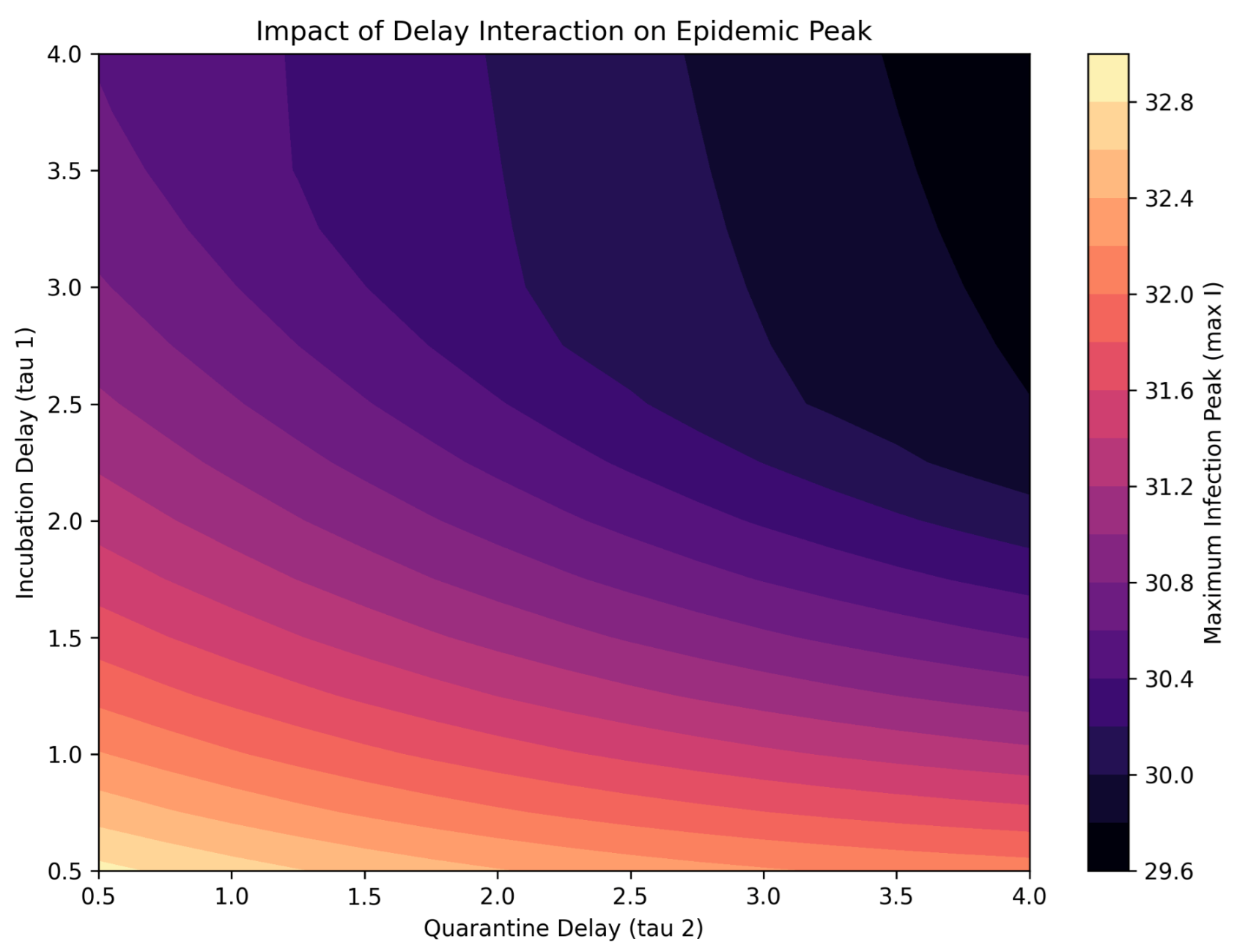
However, it should remembered that the parameters of the equation itself, such as delays, affect the peak of the epidemic. Therefore, parameter identifiability is generally not unambiguous. Let us illustrate the problem of the impact of delays on the peak of infection using a graph (Figure 5). Increasing transmission or incubation delays reduces and flattens the epidemic peak, with the strongest effect occurring when both delays are large. As we will soon explain, epidemiological models generally have too many parameters. Nevertheless, apart from biological parameters such as $\beta$, the introduced derivative parameters also have an impact on important features such as the location of the peak, the rate of increase in the number of cases, and the peak case size. We demonstrate this. A high peak poses a risk of the health care system collapsing. The slope of the ascending arm: This indicates the speed at which the epidemic is spreading (i.e., the rate of infection growth).

In a nonlinear, delayed, fractional SIQR system, the monotonicity of the epidemic peak with respect to the fractional order $\alpha$ cannot generally be guaranteed analytically without making additional assumptions on different (biological) parameters. The presented conclusions are based on the properties of fractional derivatives and the fact that the observed behavior is numerical rather than universal.

Qualitative influence of the parameters $\alpha$, $\lambda$, and $g\left(t\right)$. The generalized g-tempered fractional operator introduces three mechanisms that significantly influence the qualitative behavior of epidemic trajectories: the nonlinear temporal transformation $g\left(t\right)$, the fractional-order parameter $\alpha$, and the tempering parameter $\lambda$. The following observations provide a qualitative interpretation of their epidemiological roles.

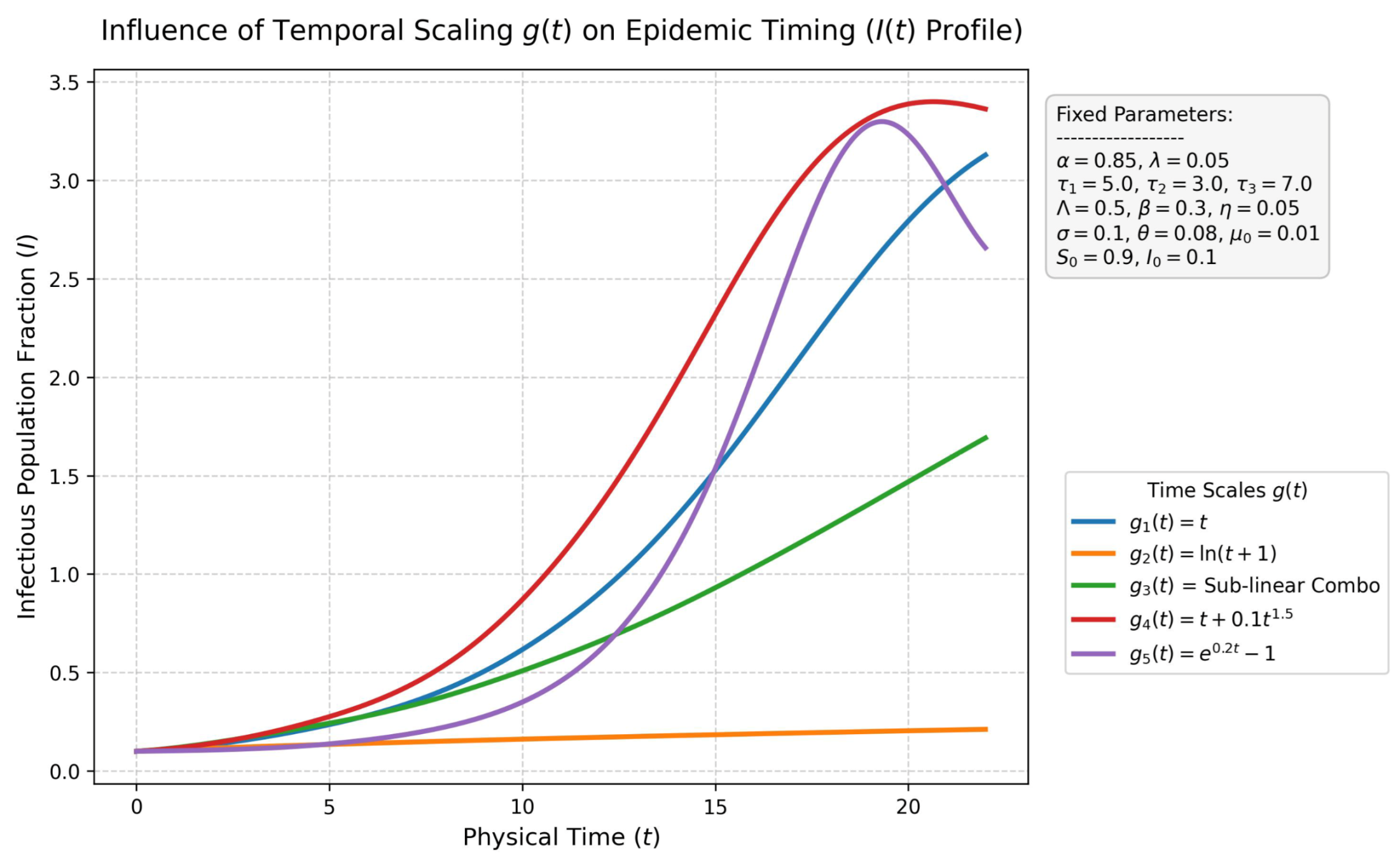
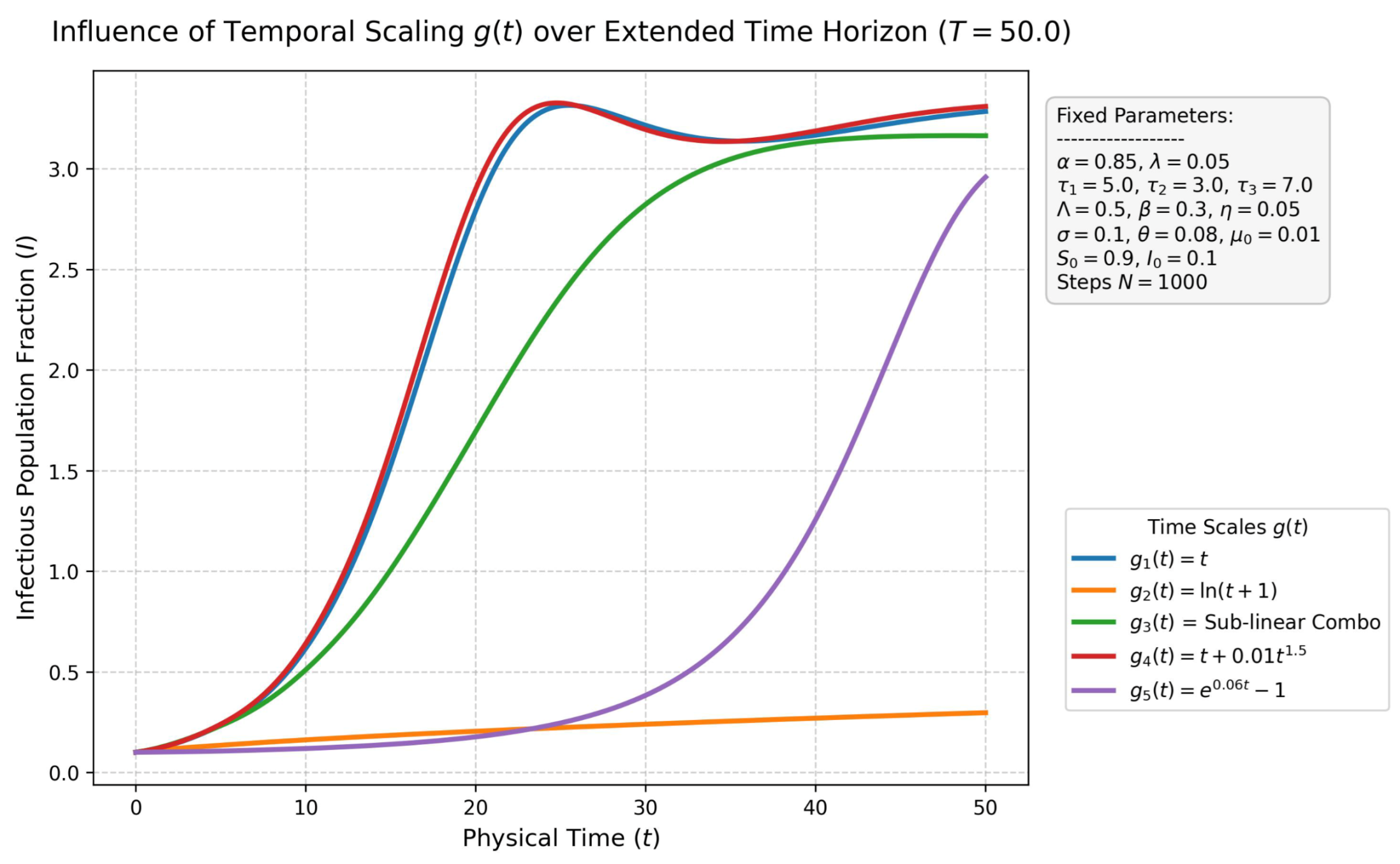
1. Influence of the temporal transformation $g\left(t\right)$ on epidemic timing. Let $s=g\left(t\right)$ denote the transformed temporal variable. Formally, using ${\displaystyle \frac{d}{dg\left(t\right)}}={\displaystyle \frac{1}{g^{\prime }\left(t\right)}}{\displaystyle \frac{d}{dt}}$, the operator may be interpreted as a tempered fractional derivative defined relative to the internal time scale s. Consequently, the function $g\left(t\right)$ modifies the correspondence between the internal epidemic dynamics and observable calendar time.

If the epidemic trajectory reaches its maximum at a biological time coordinate $s_{\mathrm{peak}}$, then the corresponding observed peak time is given by

$$t_{\max }=g^{-1}(s_{\mathrm{peak}}).$$

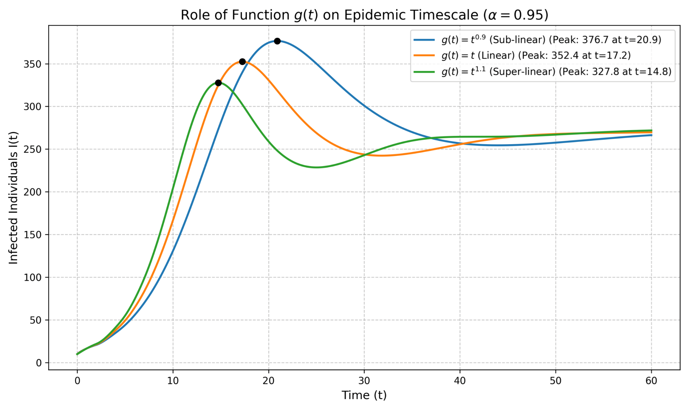
Thus, different choices of $g\left(t\right)$ may shift or deform the timing of epidemic waves in calendar time while preserving the generalized temporal structure of the model.

2. Influence of the fractional-order parameter $\alpha$ on epidemic intensity. The parameter $\alpha \in (0,1]$ controls the strength of memory effects in the system. Smaller values of $\alpha$ correspond to stronger nonlocal memory contributions, implying that the present dynamics depend more strongly on past epidemic states.

For solutions of fractional equations, the early-time asymptotic behavior is often characterized by $x(t)\sim {(g(t)-g(a))}^{\alpha }$, which yields the approximate instantaneous growth rate

$${\displaystyle \frac{d}{dt}}x(t)\sim \alpha {(g(t)-g(a))}^{\alpha -1}{g}^{\prime }(t).$$

This suggests that smaller values of $\alpha$ may produce slower transient growth and broader epidemic profiles.

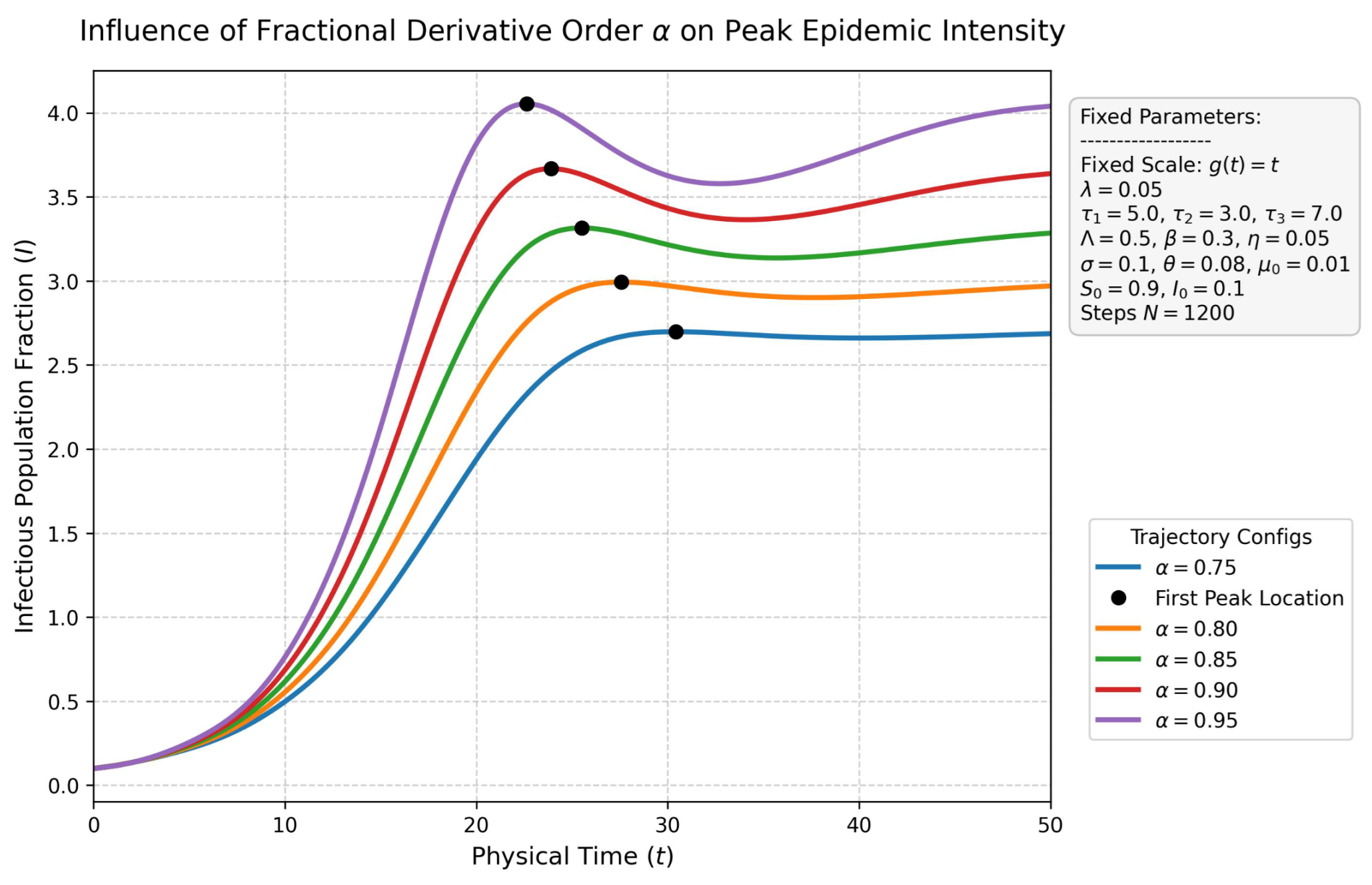
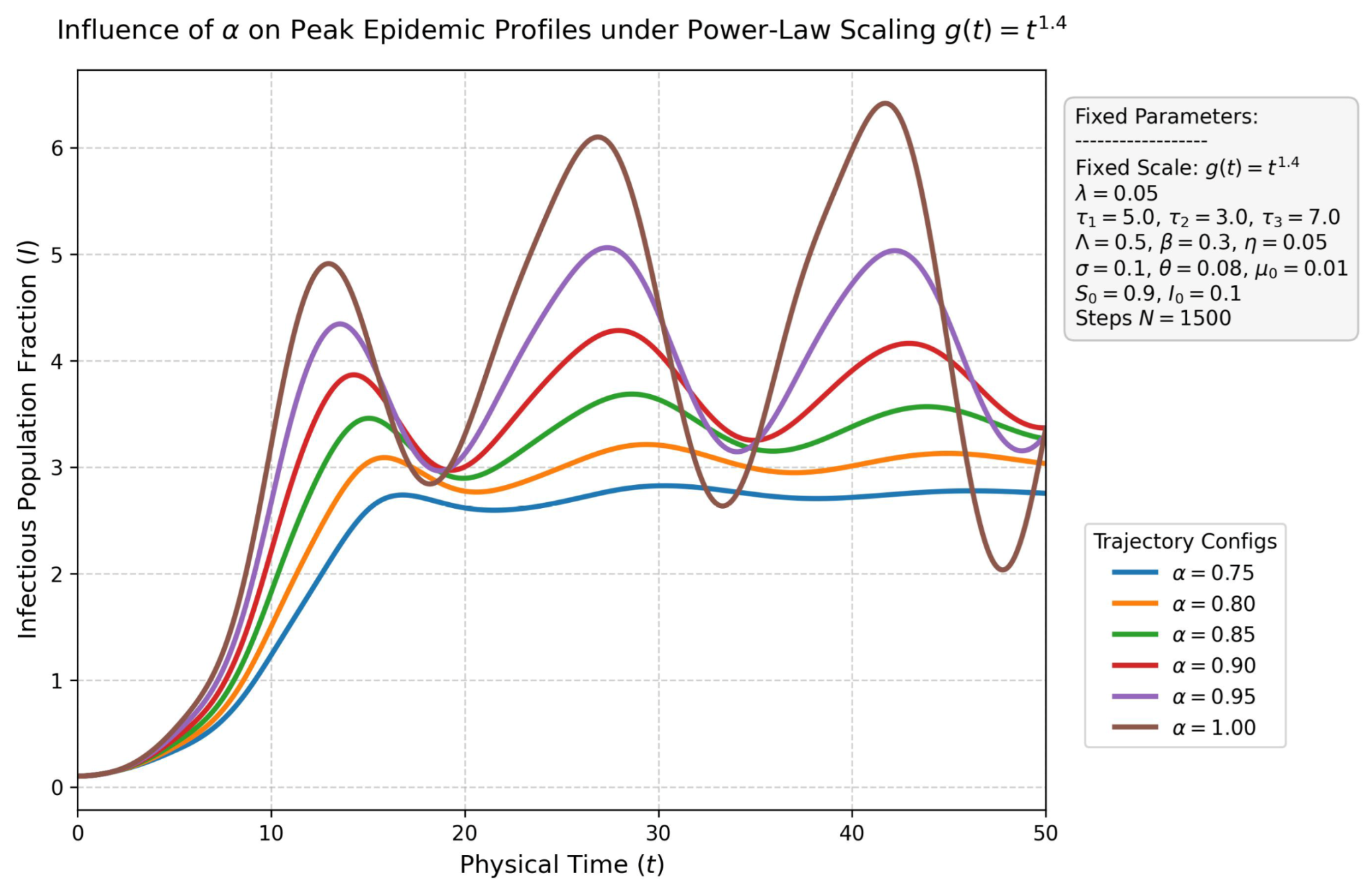
For the parameter regimes considered in the numerical simulations, decreasing values of $\alpha$ were associated with lower and wider epidemic peaks, consistent with the qualitative ‘flattening’ effect frequently observed in fractional epidemic models. However, this behavior should not be interpreted as a universal monotonic property of the full nonlinear delayed system. The peak height may depend non-trivially on additional factors, including delay parameters, transmission coefficients, initial history functions, and the temporal scaling induced by $g\left(t\right)$.

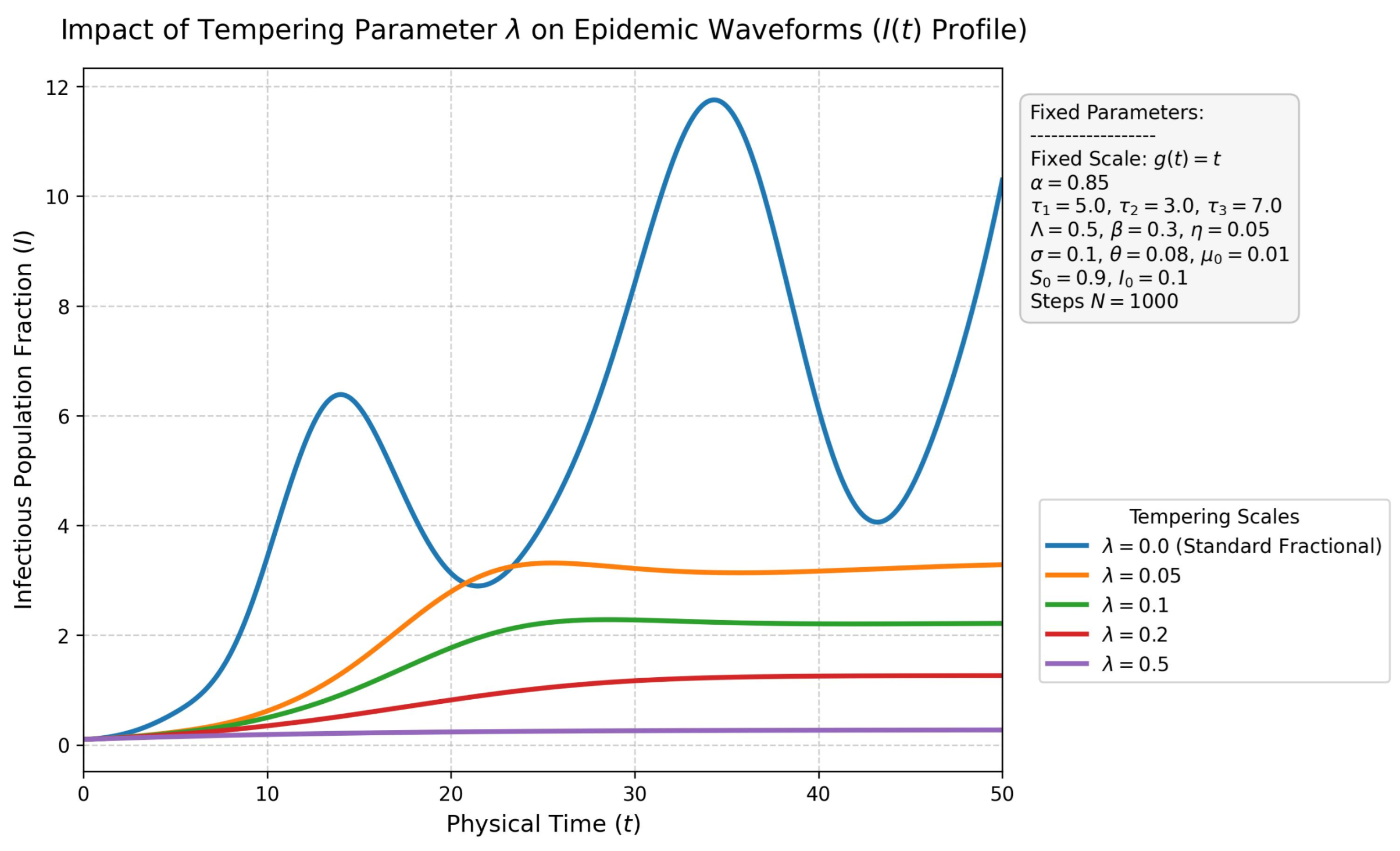
3. Influence of the tempering parameter $\lambda$ on memory persistence and convergence. Consider the memory kernel

$$K(t,s)={(g(t)-g(s))}^{\alpha -1}{e}^{-\lambda (g(t)-g(s))}.$$

For $\lambda =0$, the kernel exhibits a heavy-tailed power-law structure characteristic of standard fractional operators. Introducing $\lambda >0$ produces an exponential truncation of long-range memory effects. The effective memory capacity of the system is formally given by

$$M(t)={\int }_a^{t}K(t,s)g^{\prime }(s)ds={\int }_0^{g\left(t\right)-g\left(a\right)}{u}^{\alpha -1}{e}^{-\lambda u}du.$$

As $t\to \infty$,

$$M(t)\to {\displaystyle \frac{\Gamma \left(\alpha \right)}{{\lambda }^{\alpha }}},$$

which remains finite whenever $\lambda >0$. This indicates that the influence of distant epidemic history decays exponentially in the tempered case. Consequently, larger values of $\lambda$ reduce the effective memory horizon of the system and may accelerate convergence toward equilibrium states by suppressing persistent long-memory effects.

As claimed above, although the simulations indicate that decreasing the fractional-order parameter $\alpha$ reduces the epidemic peak $I_{\max }$, a general monotonic relationship cannot be rigorously guaranteed for the full nonlinear delayed SIQR system. In particular, the effect of $\alpha$ may interact nontrivially with other epidemiological parameters, including the transmission rate $\beta$, quarantine rate $\sigma$, recovery dynamics, and delay terms ${\tau }_i$. Consequently, different parameter regimes may exhibit qualitatively different sensitivities.

The observed flattening of the epidemic curve for smaller values of $\alpha$ should therefore be interpreted as a numerical tendency within the considered parameter set rather than as a universal mathematical property of the model. To support this observation, a numerical sensitivity analysis was performed by varying $\alpha$ while keeping the remaining parameters fixed. The simulations consistently showed a reduction in the peak magnitude and a slower epidemic evolution as $\alpha$ decreased.

This behavior is qualitatively consistent with the sub-exponential dynamics associated with fractional-order systems,

$$D_t^{\alpha }x(t)=\lambda x(t)\Rightarrow x(t)=E_{\alpha }(\lambda t^{\alpha }),$$

where the Mittag–Leffler growth function $E_{\alpha }$ exhibits slower growth than the classical exponential law for $\alpha <1$.

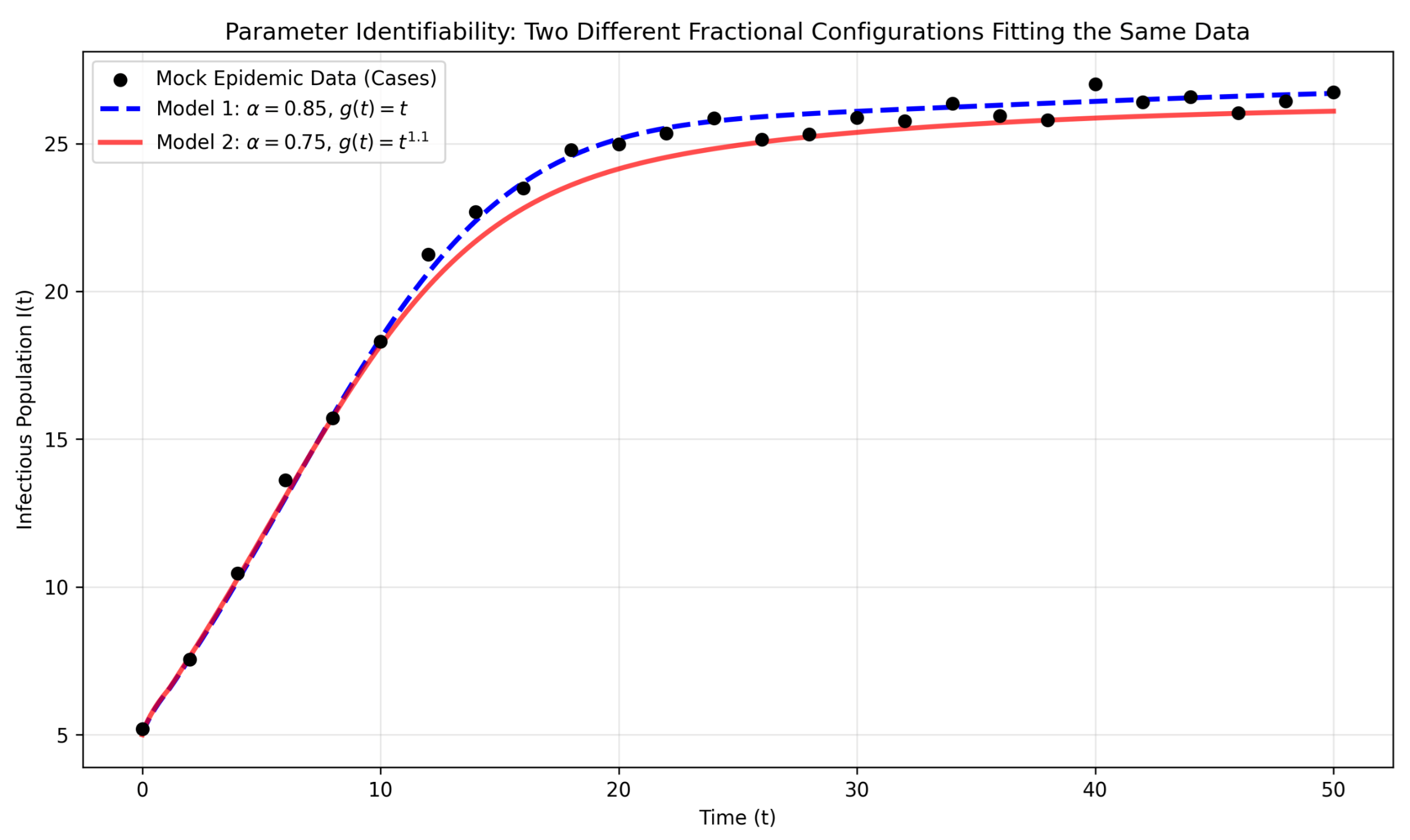
Remark 6.

The function g, together with the fractional order α, plays a key structural role in shaping the system dynamics. To illustrate this influence, we provide two representative examples. The joint identification of α and g from epidemiological observations is generally ill-posed due to structural non-identifiability. Consequently, the present study focuses on analytical properties and numerical simulations rather than full inverse problem reconstruction.

Example 1.

Delayed peak due to concave g. Suppose $g\left(t\right)=\sqrt{t}$ (concave, with $\gamma =1/2$ if we write $g\left(t\right)=t^{\gamma }$). Then $u=\sqrt{t}$, so $t=u^2$. If the standard fractional model predicts a peak at $u_{peak}=5$, then

$$t_{\max }=5^2=25.$$

In the classical case ($g\left(t\right)=t$), $t_{\max }=5$. Thus a concave g delays the peak quadratically. This models situations where effective time passes more slowly (e.g., due to interventions that stretch the epidemic).

Example 2.

Accelerated peak due to convex g. Let $g\left(t\right)=t^2$ (convex, $\gamma =2$). Then $u=t^2$, so $t=\sqrt{u}$. To keep the linear-case peak time at $t_{\max }=5$ (as in the previous example), we now need $u_{peak}=25$. Substituting gives $t_{\max }=\sqrt{25}=5$. The peak occurs earlier than in the linear case for the same $u_{peak}$ value if we had kept $u_{peak}=5$, modeling accelerated spread (e.g., superspreading events).

We will illustrate the entire problem in the final simulations, showing how to apply this approach to the analysis of data from the epidemic under study. It appears that the parameter range is specific to a given pathogen, and further research will help verify this hypothesis.

To relate these to data rigorously, we can use the necessary condition for an extremum ([45]). For a g-fractional derivative (in the Caputo sense), if $I\left(t\right)$ reaches a maximum at $t^{*}$, then ${}^C\mathcal{D}_{a,g}^{\alpha ,\lambda }I(t^{*})$ must be such that the growth halts. In a closed system, this corresponds to the point at which the ‘fractional’ reproductive number $R_t^{\alpha }=1$. To achieve this, we can investigate an equivalent fractional integral equation. At the peak $t_{max}$, the integral of the history (weighted by the integral kernel, for example, ${\left(g\right(t)-g(s\left)\right)}^{\alpha -1}$) must exactly balance the current depletion of S (see Figure 6). The peak is determined via numerical simulation (e.g., using a fractional Adams-Bashforth-Moulton method). As $\alpha$ approaches 1, the peak converges to the classical $dI/dt=0$ point.

Figure 6 illustrates the roles of the parameters $\alpha$ and $\lambda$. Next, we need to explain the role of the parameter $\lambda$ in the definition of the fractional derivative in epidemiology. The memory weight assigned to past states $x\left(s\right)$ is proportional to the tempered kernel:

$${\left(g\right(t)-g(s\left)\right)}^{\alpha -1}{e}^{-\lambda \left(g\right(t)-g(s\left)\right)}.$$

• Short-term ($t\approx s$): The term ${\left(g\right(t)-g(s\left)\right)}^{\alpha -1}$ dominates. The system behaves like a standard fractional model. This is where we see “curve flattening.”
• Long-term ($t\gg s$): The exponential term $e^{-\lambda (\dots )}$ takes over. Even if $\alpha$ is very small (suggesting strong memory), a non-zero $\lambda$ will eventually force the influence of the distant past to zero.

Epidemiological interpretation. While classical fractional derivatives assume that historical states influence the future indefinitely, introducing $\lambda$ restricts the effective memory span. In epidemiology, this accounts for system saturation or behavioral interventions (e.g., lockdowns or acquired immunity) that actively reduce the transmission potential of past cases. Consequently, $\lambda$ serves as an intervention metric: a small $\lambda$ preserves long-term memory, while a large $\lambda$ shifts the system towards classical, memoryless integer-order dynamics. In practice, a non-zero $\lambda$ can be interpreted as the rate at which containment measures reduce the effective transmission of past cases over time.

The inclusion of $\lambda$ is structurally necessary when the empirical data exhibits a prolonged plateau followed by a sudden decline. For a pure power-law decay envelope $E\left(t\right)$, the logarithmic derivative is given by ${\displaystyle \frac{d}{dt}}\log E(t)\approx -{\displaystyle \frac{\alpha }{t}}$. This magnitude strictly decreases over time, meaning that a pure fractional model cannot mathematically accelerate into a sudden drop. Conversely, the tempered model yields ${\displaystyle \frac{d}{dt}}\log E(t)\approx -{\displaystyle \frac{\alpha }{t}}-\lambda$. The constant $-\lambda$ allows the effective decay rate to remain significantly negative over time. Attempting to fit a sudden late-stage drop without the inclusion of the constant would require the value of the exponent to be artificially inflated, which would inevitably lead to overfitting and distortion of the preceding plateau phase.

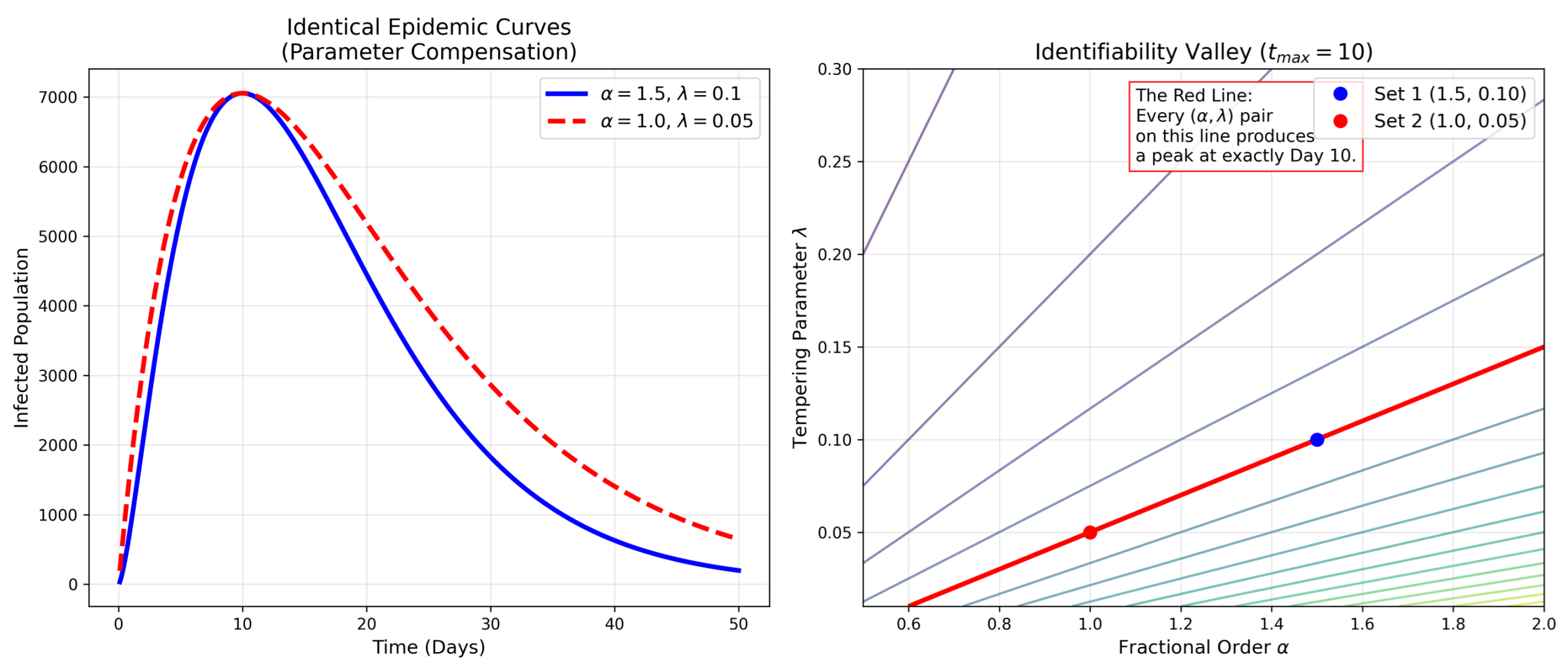
Structural non-identifiability occurs when the sensitivity of the model output $y\left(t\right)$ to $\alpha$ is nearly linearly dependent on the sensitivity to $\lambda$.

Lemma 1

(Effective Memory Horizon). For a tempered fractional system, the parameter λ defines a characteristic scale $L_{\lambda }=1/\lambda$ known as the memory horizon. For $u\ll L_{\lambda }$, the system is dominated by α. For $u\gg L_{\lambda }$, the system is dominated by λ.

Proof. 

Consider the logarithmic derivative of the kernel K with respect to the history length u:

$$\eta (u)={\displaystyle \frac{d}{du}}\ln K(u)={\displaystyle \frac{\alpha -1}{u}}-\lambda .$$

This rate of ‘forgetting’ has two distinct components:

• Fractional component: ${\displaystyle \frac{\alpha -1}{u}}$ (Dominates for small u).
• Tempering component: $-\lambda$ (Dominates for large u).

At the critical point $u^{*}={\displaystyle \frac{1-\alpha }{\lambda }}$, the two effects are equal. In epidemiological data where observations are restricted to a specific phase (e.g., only the peak or only the early decay), the data often does not span enough of the u-domain to distinguish between a change in the power-law slope ($\alpha$) and a change in the exponential truncation ($\lambda$).  □

The memory horizon $L_{\lambda }$ serves as a fundamental limit for parameter identifiability. Our results suggest that, unless the observation period T exceeds this characteristic scale, the sensitivity functions $J-\alpha$ and $J_{\lambda }$ remain approximately collinear. Therefore, any ’optimal’ parameter set identified within short-term windows should be considered representative of a solution manifold rather than a unique biological truth.

In biological terms, $L_{\lambda }$ represents the effective window of relevance for past infection spikes. It filters out ’stale’ information, such as the initial seeding event, enabling the SIQR model to concentrate on recent quarantine (Q) and recovery (R) rates. This provides a more realistic representation of ’fatigue’ in social interventions and viral clearance than classical infinite-memory models.

Timeline of the Epidemic

Now, we need to focus on both the peak of the outbreak and the epidemic’s entire duration. The next step is based on the use of an auxiliary parameter: the function g. This function enables us to transition from global memory (standard fractional derivative) to warped memory (g-fractional) and filtered memory (tempered). Combining tempering (exponential forgetting) and warping (non-linear time flow) creates a model that accounts for the biological decay of memory and the social/environmental acceleration of time.

In a standard dynamical system, we assume time flows uniformly ($g\left(t\right)=t$). By introducing $g\left(t\right)$, we can essentially ‘stretch’ or ‘compress’ the fabric of time before applying the memory kernel.

In classical compartmental epidemiological models, such as the SIR framework, model parameters possess clear physical interpretations and well-defined temporal units. For example, transmission and recovery rates are typically expressed in units of ${\left[T\right]}^{-1}$, corresponding to rates per unit of calendar time (e.g., day⁻¹).

In contrast, the g-fractional operator ${}^C\mathcal{D}_{a,g}^{\alpha ,\lambda }$ is defined relative to the transformed time scale $g\left(t\right)$. Consequently, the dimensional structure of the model is governed by the generalized differential measure $dg\left(t\right)$ rather than the classical differential $dt$, placing the formulation within the broader class of Stieltjes-type fractional operators (cf. [6]). The epidemiological interpretation of the model parameters therefore depends on the scaling properties of $g\left(t\right)$, and relating inferred quantities to observable calendar-time data requires an explicit correspondence between $g\left(t\right)$ and physical time.

To preserve epidemiological interpretability, we assume that $g\left(t\right)$ is monotone increasing and normalized so that it has the dimension of time. Under this assumption, the parameters $\beta ,\sigma$, and $\eta$ retain the standard units day⁻¹, while the delay parameter $\tau$ is expressed in days. The fractional-order parameter $\alpha \in (0,1]$ remains dimensionless and characterizes the strength of memory effects in the transmission dynamics.

Fractional-order derivatives are inherently non-local operators by definition, as their evaluation depends explicitly on the initial time point a. In the context of the g-tempered derivative, the memory kernel is effectively anchored at the transformed time $g\left(a\right)$, rather than at a itself. This distinction introduces additional complexity when the mapping $g\left(t\right)$ is nonlinear. Notably, if $g\left(t\right)$ exhibits slow growth near the initial time, for example, in the case $g\left(t\right)=t^{\gamma }$ with $0<\gamma <1$, the system evolves very gradually in effective time during the early phase. This behavior poses a significant modeling challenge in that it makes the model highly sensitive to the choice of the initial time a. Small inaccuracies in estimating the onset of the epidemic can be amplified considerably by the nonlinear transformation induced by $g\left(t\right)$. Consequently, even minor errors in the initial time a can propagate into significant deviations in the predicted temporal evolution, potentially altering key features of the epidemic trajectory, such as peak timing, by several weeks.

We discussed the tempering role of the parameter $\lambda$. This governs the rate at which the system loses memory of past states. In the case of the g-tempered fractional derivative, this memory decay occurs with respect to an effective time scale rather than standard calendar time. Consequently, the evolution of memory is directly influenced by the choice of the function g. When g represents an intervention mechanism, such as a lockdown function characterized by intervals of constancy, the progression of effective time is significantly altered. Notably, during periods when $g\left(t\right)$ remains nearly constant, the increment $g\left(t\right)-g\left(s\right)$ grows very slowly or not at all. Consequently, the system exhibits reduced memory decay when measured against real (calendar) time. This phenomenon introduces a critical modeling issue, referred to here as the frozen memory effect. Under such conditions, the system retains a disproportionately strong dependence on its pre-intervention state over an extended period of physical time. This persistence may lead to unrealistic dynamics, as the model fails to adequately reflect the natural attenuation of past influences during prolonged intervention periods. Analyzing slowly growing functions (including statistical ones) requires particular care, and high-precision numerical simulations are necessary.

Remark 7.

It is worth noting that the assumption that the function g is $C^1$ smooth allows us to account for interesting memory effects. However, one can imagine epidemiological phenomena that go beyond this theory. A full description of, for example, a frozen epidemic data (a lockdown) requires a function g being piecewise continuous or regulated functions (see [6]).

Suppose that a containment policy (e.g., a lockdown) is introduced at time $T_c$. This still can be modeled using a scale function g

$$g\left(t\right)=t\chi \left([a,T_c]\right)\left(t\right)+[T_c+k(t-T_c)]\chi \left([T_c,b]\right)\left(t\right),$$

where k is a reduction factor for social activity and ${\chi }_A$ is the characteristic function of A. Although $g\notin C^1\left([a,b]\right)$, the fractional integral $I_{a,g}^{\alpha ,\lambda }$ remains well-defined because g is strictly increasing. The term $g^{\prime }\left(s\right)$ in the integral can be interpreted in the sense of Lebesgue almost everywhere, or more generally in terms of Stieltjes integrals. It leads to the analysis of models with non-continuous solutions, as described in [6]. This approach is mathematically cleaner than using time-dependent parameters $\beta \left(t\right)$, as it attributes the change to the flow of interaction time rather than to a change in the virus itself. Unfortunately, this requires a construction based on Stieltjes integrals and derivatives. We will not discuss this theory in detail here. However, as discussed in [46], Baker and Paul were the first to demonstrate the feasibility and validity of discontinuous solutions in delayed models. Subsequently, in the paper [47], it is proposed to preserve past discontinuities using a different Stieltjes-type integral. Those interested in the fundamentals of constructing such models in epidemiology are referred to [6] (for the case where $\alpha =1$).

Lemma 2

(Operator Equivalence under Time-Warping). Let $g:[a,b]\to \left[g\right(a),g(b\left)\right]$ be a strictly increasing $C^1$ function. For any differentiable function $x\left(t\right)$, the g-tempered Caputo operator is equivalent to a standard tempered Caputo operator acting on the warped state $\tilde{x}\left(u\right)=x\left(g^{-1}\right(u\left)\right)$ in the u-domain:

$$\left({}^C\mathcal{D}_{a,g}^{\alpha ,\lambda }x\right)\left(t\right)=\left({}^C\mathcal{D}_{g\left(a\right)}^{\alpha ,\lambda }\tilde{x}\right)\left(u\right){|}_{u=g\left(t\right)}.$$

Proof. 

Starting from the integral definition:

$$\left({}^C\mathcal{D}_{a,g}^{\alpha ,\lambda }x\right)\left(t\right)={\displaystyle \frac{1}{\Gamma (1-\alpha )}}{\int }_a^t{\left(g\right(t)-g(s\left)\right)}^{-\alpha }{e}^{-\lambda \left(g\right(t)-g(s\left)\right)}{\displaystyle \frac{dx\left(s\right)}{dg\left(s\right)}}dg(s).$$

Perform the change of variables $v=g\left(s\right)$, which implies $dv=dg\left(s\right)$. When $s=a$, $v=g\left(a\right)$; when $s=t$, $v=g\left(t\right)=u$. The term ${\displaystyle \frac{dx\left(s\right)}{dg\left(s\right)}}$ becomes ${\displaystyle \frac{d\tilde{x}\left(v\right)}{dv}}$ by the chain rule. Substituting these into the integral:

$${\displaystyle \frac{1}{\Gamma (1-\alpha )}}{\int }_{g\left(a\right)}^u{(u-v)}^{-\alpha }{e}^{-\lambda (u-v)}{\tilde{x}}^{\prime }(v)dv.$$

This is precisely the definition of the standard tempered Caputo derivative ${}^C\mathcal{D}^{\alpha ,\lambda }$ acting on $\tilde{x}$ with respect to the variable v over the interval $\left[g\right(a),u]$.  □

Remark 8.

While Lemma 2 establishes the invariance of the differentiation operator, it is crucial to note that the SIQR system as a whole is not invariant under a constant delay shift in the u-domain. Specifically, a constant calendar delay τ in the physical time t transforms into a time-dependent delay in the warped domain u:

$$x(t-\tau )=\tilde{x}\left(g(g^{-1}(u)-\tau )\right).$$

In the warped u-variable, the delay is no longer the constant τ unless $g\left(t\right)$ is a linear function. Therefore, the qualitative analysis of the g-fractional delayed system must account for this non-linear mapping of the history segment.

Remark 9.

The loss of direct interpretability of epidemiological parameters in the g-fractional SIQR model poses a significant challenge to its practical application. In particular, the non-linear reparameterisation of time via the transformation $g\left(t\right)$ obscures the physical meaning of important quantities such as the transmission and recovery rates, which are no longer expressed per unit of calendar time.

Although the g-fractional formulation provides additional flexibility for modeling memory and nonlocal effects, it also modifies the temporal interpretation of epidemiological parameters. As claimed before, in classical compartmental models, such as the SIR or SIQR systems, transmission and recovery rates are typically expressed per unit of calendar time (e.g., day⁻¹). In contrast, the operator ${}^C\mathcal{D}_{a,g}^{\alpha ,\lambda }$ is defined with respect to the transformed time scale $g\left(t\right)$, so that the effective differential structure is governed by $dg\left(t\right)$ rather than $dt$.

Consequently, model parameters are naturally interpreted relative to the generalized time variable $g\left(t\right)$. To relate the model outputs to observable epidemiological data indexed in calendar time, an explicit correspondence between $g\left(t\right)$ and physical time must therefore be specified. Assuming that $g\left(t\right)$ is monotone increasing and sufficiently smooth, the transformation $s=g\left(t\right)$ allows the system to be expressed in terms of an effective time variable s. Epidemiological quantities reported in calendar time may then be recovered through the inverse mapping $t=g^{-1}\left(s\right)$, whenever the inverse exists.

A partial interpretation in calendar time may be obtained through local parameter rescaling. Formally, the quantities

$$\tilde{\beta }(t)=\beta g^{\prime }(t),\tilde{\gamma }(t)=\gamma g^{\prime }(t),$$

can be viewed as effective instantaneous rates with respect to physical time. However, in the fully fractional setting this rescaling does not completely characterize the dynamics, since the memory kernel of the g-fractional operator depends non-locally on the transformed temporal metric induced by $g\left(t\right)$. Consequently, the epidemiological interpretation of the parameters cannot, in general, be reduced to a purely local time-dependent reparameterization. The quantities $\tilde{\beta }(t)$ and $\tilde{\gamma }(t)$ may be interpreted as effective local-in-time rates relative to calendar time. However, this interpretation is only partial, since the full g-fractional dynamics remain governed by a nonlocal memory kernel depending on the transformed temporal metric induced by $g\left(t\right)$.

For practical applications, the choice of the transformation function $g\left(t\right)$ should be guided by empirical or physical considerations. In particular, selecting $g\left(t\right)$ to reflect measurable temporal heterogeneity, such as cumulative contact activity or mobility-adjusted time, improves the interpretability of the inferred parameters and facilitates calibration against epidemiological data recorded in calendar time. The choice of the transformation function $g\left(t\right)$ should be guided by empirical or physical considerations. Rather than adopting arbitrary functional forms, it is preferable to select $g\left(t\right)$ so that it reflects a measurable or interpretable process, such as cumulative contact intensity or mobility-adjusted time. Under such a formulation, rates defined with respect to $g\left(t\right)$ retain an indirect, yet meaningful, connection to real-world dynamics.

A hybrid modeling strategy may be employed to bridge the gap between theoretical generality and practical usability. In this approach, the g-fractional model is used to capture memory effects and complex temporal behavior, while an equivalent, or, in practice, approximate, classical model with time-varying parameters is constructed for reporting and interpretation. This facilitates communication of results in terms familiar to public health practitioners without sacrificing the advantages of the fractional framework. Calibrating against empirical data indexed in calendar time is essential. Fitting the model directly to observed epidemiological time series, one ensures consistency with real-world temporal patterns. While this does not completely solve the problem of parameter identifiability, it reduces ambiguity in interpretation and improves the reliability of model-based predictions.

5. General Model

In epidemiology, all models can be represented as a system of differential equations with a nonlinear, typically vector, right-hand side. We will therefore first present the abstract form of the proposed model, followed by several special cases and a flowchart illustrating how to apply this to any desired model. Consider the vector-valued formulation of the system in question:

$$\mathbf{x}(t)=\left[\begin{array}{c}{x}_1(t)\\ x_2(t)\\ x_3(t)\\ x_4(t)\end{array}\right]$$

(8)

(the number of variables is dependent on the number of equations in the system). Moreover, the initial value is given by

$${\mathbf{x}}_0=\left[\begin{array}{c}{x}_1(0)\\ x_2(0)\\ x_3(0)\\ x_4(0)\end{array}\right].$$

(9)

Let $X(t)={\left[S\right(t),I(t),Q(t),R(t\left)\right]}^T\in {\mathbb{R}}^4$. We define the nonlinear functional F: ${\left({\mathbb{R}}^4\right)}^4\to {\mathbb{R}}^4$ as:

$$\begin{array}{ccc}& & F\left(X\right(t),X(t-{\tau }_1),X(t-{\tau }_2),X(t-{\tau }_3\left)\right)\hfill \\ & =& \left(\begin{array}{c}ł\Lambda -\beta S\left(t\right)I(t-{\tau }_1)-{\mu }_{0}S\left(t\right)\\ \beta S\left(t\right)I(t-{\tau }_1)+\eta R\left(t\right)I(t-{\tau }_1)-\sigma I(t-{\tau }_2)-{\mu }_{0}I\left(t\right)\\ \sigma I(t-{\tau }_2)-\theta Q(t-{\tau }_3)-{\mu }_{0}Q\left(t\right)\\ \theta Q(t-{\tau }_3)-\eta R\left(t\right)I(t-{\tau }_1)-{\mu }_{0}R\left(t\right)\end{array}\right).\hfill \end{array}$$

The fractional-order SIQR system can then be written compactly as:

$${}^C\mathcal{D}_{a,g}^{\alpha ,\lambda }X(t)=F(X(t),X(t-{\tau }_1),X(t-{\tau }_2),X(t-{\tau }_3)).$$

Specifically, for the SIQR model we consider the state vector:

$$\mathbf{x}(t)={\left(x_1\right(t),x_2(t),x_3(t),x_4(t\left)\right)}^T={\left(S\right(t),I(t),Q(t),R(t\left)\right)}^T.$$

In general, for any four-compartment epidemiological model (such as the SEIR model where $\mathbf{x}(t)={\left(S\right(t),E(t),I(t),R(t\left)\right)}^T$), the dynamics can be expressed by the vector-valued equation:

$${}^C\mathcal{D}^{\alpha ,\lambda }a,g\mathbf{x}(t)=F(\mathbf{x}(t),\mathbf{x}(t-{\tau }_1),\mathbf{x}(t-{\tau }_2),\mathbf{x}(t-{\tau }_3)),$$

(10)

where ${}^C\mathcal{D}^{\alpha ,\lambda }a,g$ denotes the considered tempered fractional derivative with respect to the scaling function g.

Moreover, since we investigate a delay differential problem, we require an initial condition given by a function $\psi \in \mathcal{B}$, so in this case usually

$$\psi \in C([-r,0],{\mathbb{R}}^4),\mathrm{where}r=\max \{{\tau }_1,{\tau }_2,{\tau }_3\},$$

such that

$$\mathbf{x}\left(t\right)=\psi \left(t\right),t\in [-r,0].$$

(11)

For the case of continuous solutions we can put $\mathcal{B}=C([-r,0],{\mathbb{R}}^4)$, but this result is more general, and contains the case of discontinuous solutions, i.e., with $\mathcal{B}$ being a subspace of regulated functions (see [6]).

In order to perform numerical simulations of the SIQR model (or any other model), we must first prove the general theorem concerning the existence and uniqueness of solutions.

Let $\mathcal{B}$ be a Banach space of functions $\varphi :[-\tau ,0]\to {\mathbb{R}}^n$ with norm ${\parallel ·\parallel }_{\mathcal{B}}$. Assume that $\mathbf{F}:[0,\infty )\times \mathcal{B}\to {\mathbb{R}}^n$ satisfies:

(H1)

The map $t\mapsto \mathbf{F}(t,\psi )$ is continuous for every $\psi \in \mathcal{B}$.

(H2)

For every $M>0$, there exists $L_M>0$ such that for all ${\psi }_1,{\psi }_2\in \mathcal{B}$ with

${\parallel {\psi }_1\parallel }_{\mathcal{B}},{\parallel {\psi }_2\parallel }_{\mathcal{B}}\le M$,

$$\parallel \mathbf{F}(t,{\psi }_1)-\mathbf{F}(t,{\psi }_2)\parallel \le L_M{\parallel {\psi }_1-{\psi }_2\parallel }_{\mathcal{B}}.$$

(H3)

There exist constants $k,l\ge 0$ such that

$$\parallel \mathbf{F}(t,\psi )\parallel \le k+{l\parallel \psi \parallel }_{\mathcal{B}}\mathrm{for}\mathrm{all}(t,\psi )\in [0,\infty )\times \mathcal{B}.$$

(H4)

If $\psi \in \mathcal{B}$ satisfies $\psi \left(\theta \right)\in {\mathbb{R}}_{+}^n$ for all $\theta \in [-\tau ,0]$ and ${\psi }_i\left(0\right)=0$, then

$${\mathbf{F}}_i(t,\psi )\ge 0\mathrm{for}\mathrm{all}t\ge 0.$$

(H5)

There exists a constant vector $\mathbf{c}\in {\mathbb{R}}^n$ with $c_i>0$, and constants $\Lambda >0,\mu >0$ such that for all $(t,\psi )\in [0,\infty )\times \mathcal{B}$:

$${\displaystyle \sum _{i=1}^n}{c}_i{\mathbf{F}}_i(t,\psi )\le \Lambda -\mu \left({\displaystyle \sum _{i=1}^n}{c}_i{\psi }_i(0)\right).$$

It seems necessary to make a comment about (H5). The SIQR system is dissipative, but not bounded. While the delayed transitions ${\tau }_i$ prevent terms in the sum ${\mathbf{F}}_i$ from being cancelled out directly, we observe that, for any $t>max\left({\tau }_i\right)$, the delayed terms represent internal transfers within the population. As the natural death rate ${\mu }_0$ applies to all compartments and the recruitment d is constant, the total population $N\left(t\right)$ is governed by the functional inequality:

$${}^C\mathcal{D}_{a,g}^{\alpha ,\lambda }N(t)\le \Lambda -{\mu }_{0}N(t)+\mathcal{R}(t),$$

where $\mathcal{R}\left(t\right)$ accounts for the delayed history. Since the history $\varphi$ is bounded on $[-\tau ,0]$, by the comparison theorem for fractional differential equations, $N\left(t\right)$ remains bounded for all $t\in [0,\infty )$. In our SIQR model, (H5) is satisfied by taking $c_i=1$, as the delayed transition terms represent internal flux and the total population is bounded by the natural mortality rate.

Theorem 1.

Consider the vector-valued system ${}^C\mathcal{D}_{a,g}^{\alpha ,\lambda }x(t)=\mathbf{F}(t,x_t)$ with the initial history $x_0=\varphi \in \mathcal{B}$, where $\mathcal{B}=C([-\tau ,0],{\mathbb{R}}_{+}^n)$. Under assumptions (H1)–(H5), there exists a unique global solution $x\in C([-\tau ,\infty ),{\mathbb{R}}_{+}^n)$ such that:

(i) 

$x_0=\varphi$,

(ii) 

The solution $x\left(t\right)$ is unique and depends continuously on the initial data,

(iii) 

The solution $x\left(t\right)$ remains in the positive orthant ${\mathbb{R}}_{+}^n$ for all $t\ge 0$.

Proof. 

The proof is divided into four distinct phases: equivalence, local existence via fixed-point theory, global existence, and non-negativity.

Step 1: Integral Representation. Applying the g-tempered fractional integral $I_{a,g}^{\alpha ,\lambda }$ (cf. (5) and (6)) to both sides of the system, we obtain the equivalent Volterra-type integral equation:

$$x(t)=\left\{\begin{array}{cc}\varphi \left(t\right),\hfill & t\in [-\tau ,0],\hfill \\ \varphi (0)+{\displaystyle \frac{1}{\Gamma \left(\alpha \right)}}{\int }_0^t{e}^{-\lambda \left(g\right(t)-g(s\left)\right)}{\left(g\right(t)-g(s\left)\right)}^{\alpha -1}{g}^{\prime }(s)\mathbf{F}(s,x_s)ds,\hfill & t\in [0,T],\hfill \end{array}\right.$$

(12)

where $x_s$ denotes the segment of the solution representing the history $[s-\tau ,s]$.

Step 2: Local Existence and Uniqueness. Let $T>0$ and define the space of solutions $E=C([-\tau ,T],{\mathbb{R}}^n)$ with the supremum norm ${\parallel ·\parallel }_E$. We define an operator $\mathcal{P}:E\to E$ based on the right-hand side of Equation (12). For any $x,y\in E$ such that $\parallel x\parallel ,\parallel y\parallel \le M$, assumption (H2) implies:

$$\begin{array}{ccc}\hfill \parallel \mathcal{P}x\left(t\right)-\mathcal{P}y\left(t\right)\parallel & \le & {\displaystyle \frac{L_M}{\Gamma \left(\alpha \right)}}{\int }_0^t{e}^{-\lambda \left(g\right(t)-g(s\left)\right)}{(g(t)-g(s))}^{\alpha -1}{g}^{\prime }(s){\parallel x_s-y_s\parallel }_{\mathcal{B}}ds\hfill \\ & \le & {\displaystyle \frac{L_M{|x-y|}_E}{\Gamma \left(\alpha \right)}}{\int }_0^t{(g(t)-g(s))}^{\alpha -1}{g}^{\prime }(s)ds\hfill \\ & \le & {\displaystyle \frac{L_M{(g(t)-g(0))}^{\alpha }}{\Gamma (\alpha +1)}}{\parallel x-y\parallel }_E.\hfill \end{array}$$

By choosing a sufficiently small T such that ${\displaystyle \frac{L_M{(g(T)-g(0))}^{\alpha }}{\Gamma (\alpha +1)}}<1$, the operator $\mathcal{P}$ becomes a contraction mapping. By the Banach fixed point theorem, a unique local solution exists on $[0,T]$.

Step 3: Global Boundedness (Verification of (H5)). To establish that the solution $x\left(t\right)$ is global, we must show it does not blow up in finite time. Define a Lyapunov-like function $V(x(t))={\sum }_{i=1}^n{c}_i{x}_i\left(t\right)$. By the linearity of the g-tempered fractional operator and assumption (H5), we have:

$$\begin{array}{ccc}\hfill {}^C\mathcal{D}_{a,g}^{\alpha ,\lambda }V(x(t))& =& {\displaystyle \sum _{i=1}^n}{c}_i\hfill \\ \hfill {}^C\mathcal{D}_{a,g}^{\alpha ,\lambda }{x}_i(t)& =& {\displaystyle \sum _{i=1}^n}{c}_i{\mathbf{F}}_i(t,x_t).\hfill \end{array}$$

Applying the inequality from (H5), it follows that:

$${}^C\mathcal{D}_{a,g}^{\alpha ,\lambda }V(x(t))\le \Lambda -\mu V(x(t)).$$

Let $z\left(t\right)$ be the solution to the auxiliary equation ${}^C\mathcal{D}_{a,g}^{\alpha ,\lambda }z(t)=\Lambda -\mu z(t)$ with $z\left(a\right)=V\left(\mathbf{x}\right(a\left)\right)$. By the Comparison Principle for g-tempered fractional derivatives (cf. [48]), we have $V\left(\mathbf{x}\right(t\left)\right)\le z\left(t\right)$ for all $t\ge a$. The solution $z\left(t\right)$ is given by:

$$z\left(t\right)=z\left(a\right)E_{\alpha ,1}\left(-\mu {(g\left(t\right)-g(a\left)\right)}^{\alpha }\right)+\Lambda {\left(g\right(t)-g(a\left)\right)}^{\alpha }{E}_{\alpha ,\alpha +1}\left(-\mu {\left(g\right(t)-g(a\left)\right)}^{\alpha }\right),$$

(13)

where $E_{\alpha ,\beta }$ is the two-parameter Mittag-Leffler function. Since $E_{\alpha ,\beta }$ is bounded on the positive real axis for $\mu >0$, there exists a constant $M>0$ such that $V\left(\mathbf{x}\right(t\left)\right)\le M$. Given that $c_i>0$ and $x_i\left(t\right)\ge 0$ (from Step 3), this implies that each component $x_i\left(t\right)$ is bounded. Due to the linear growth condition (H3) and boundedness (H5), this solution is global, so it can be extended to the interval $[0,\infty )$.

Step 4: Non-negativity of solutions. We prove that $x\left(t\right)\in {\mathbb{R}}_{+}^n$ for all $t\ge 0$ by contradiction.

Suppose there exists a time $t>0$ such that the solution leaves the positive orthant. Let $t_c$ be the first time at least one component of the solution reaches zero:

$$t_c=\inf \{t>0:\exists i\in \{1,\dots ,n\}\mathrm{such}\mathrm{that}{x}_i(t)=0\}.$$

By the continuity of the solution and the definition of the infimum, we have $x_i\left(t_c\right)=0$ and $x_j\left(t\right)\ge 0$ for all $j\in \{1,\dots ,n\}$ on the interval $[0,t_c]$. Furthermore, for the specific component i, it must hold that $x_i\left(t\right)>0$ for $t\in [0,t_c)$, meaning $t_c$ is a point of local minimum for $x_i$ on $[0,t_c]$.

According to the generalized extremum principle ([45,49]) for the g-tempered Caputo fractional derivative, if a function $x_i\left(t\right)\in C[0,t_c]$ attains its minimum over $[0,t_c]$ at the point $t_c$, then its g-tempered fractional derivative at that point satisfies:

$${}^C\mathcal{D}_{a,g}^{\alpha ,\lambda }{x}_i\left(t_c\right)\le 0.$$

(14)

Intuitively, since $x_i\left(t\right)$ is decreasing toward zero or has remained above zero in the past, the weighted memory of the derivative pulls the value downward or stays neutral. Conversely, evaluating the system dynamics at $t=t_c$, we utilize the vector field $\mathbf{F}$. Given that the history segment $x_{t_c}$ satisfies $x_{t_c}\left(\theta \right)\in {\mathbb{R}}_{+}^n$ for all $\theta \in [-\tau ,0]$ and the current state satisfies $x_i\left(t_c\right)=0$, the quasi-positivity assumption (H4) implies:

$${}^C\mathcal{D}_{a,g}^{\alpha ,\lambda }{x}_i\left(t_c\right)={\mathbf{F}}_i(t_c,x{t}_c)\ge 0.$$

(15)

Comparing (14) and (15), the only consistent value is ${}^C\mathcal{D}_{a,g}^{\alpha ,\lambda }{x}_i\left(t_c\right)=0$. If ${\mathbf{F}}_i(t_c,x_{t_c})>0$, we reach an immediate contradiction. If ${\mathbf{F}}_i(t_c,x_{t_c})=0$, the uniqueness of the solution (established in Step 2) ensures that the trajectory cannot cross the boundary $\{x_i=0\}$ into the negative region. Therefore, $x\left(t\right)$ remains in ${\mathbb{R}}_{+}^n$ for all $t\ge 0$.  □

It is easily verified that the right-hand side of the SIQR model satisfies the Lipschitz and quasi-positivity conditions (H2) and (H4) due to its polynomial structure and the positivity of $\Lambda$. Furthermore, summing the equations yields a uniform bound on the total population, implying assumption (H5). Therefore, according to Theorem 1, the model has a unique global nonnegative solution. More generally, epidemiological models are well-posed due to their locally Lipschitz (mechanistic interactions), quasi-positive (biological) and dissipative (finite population) properties.

In practice, the spread of infectious diseases is influenced by a variety of factors, such as behavioral changes, intervention strategies and environmental conditions. Traditional mathematical models often assume constant parameters to maintain analytical tractability and simplify the governing equations. While this is convenient, it can limit the model’s ability to accurately reflect complex, time-varying dynamics. In contrast, the proposed framework introduces additional flexibility by enabling the progression of time to be modulated via the function $g\left(t\right)$. This enables heterogeneous effects on disease transmission and progression to be incorporated, effectively embedding multiple influencing factors into the temporal structure of the model. By selecting the appropriate form of $g\left(t\right)$, along with other model parameters, the system can be calibrated to align more closely with empirical observations across different diseases and environmental settings. Consequently, the model provides a more adaptable and realistic representation of epidemic dynamics.

For the sake of clarity, let us recall that the proposed derivative approach covers many others and there is no need to examine them separately. Let’s gather a few known cases and indications in a table, along with when they could be used.

Table 7. Special cases of fractional calculus for different functions g.

$\mathit{g}\left(\mathit{t}\right)$	Derivative Type	Memory Kernel	Data Application
$g\left(t\right)=t$	Riemann-Liouville/Caputo	Power-law $t^{-\alpha }$	Standard fractional models
$g\left(t\right)=\ln t$	Hadamard-type	Logarithmic	Data with slow variation
$g\left(t\right)=t^{\beta }$	Erdélyi-Kober	Generalized power-law	Multi-scale dynamics
$g\left(t\right)=e^t$	Exponential kernel	Rapidly decaying memory	Short-term memory effects

shows that our approach covers several known cases.

6. Ill-Posedness of the Inverse Problem

One of the practical problems associated with the analysis of epidemiological data that remains to be discussed is the possibility of adjusting the model parameters to a given set of data. The method of reducing the number of parameters in order to determine the remaining ones is already well-known in the case of biological factors (e.g., [50]). As with all our paper, our focus will be on the parameters of the derivative. We add three more parameters, including one function. The challenge lies in demonstrating that even with established biological parameters, the problem of reproducing those parameters based on the model solution is ill-posed. As with biological parameters, statistical analysis and numerical simulations can help here. This is a new and very broad topic, so here we will outline the basic methods and facts here, encouraging readers to verify them on their own datasets.

In the g-tempered fractional SIQR model, the memory kernel is defined as:

$$K(u;\alpha ,\lambda )=u^{\alpha -1}{e}^{-\lambda u},\mathrm{where}u=g(t)-g(s).$$

The structural identifiability of the parameter pair $(\alpha ,\lambda )$ is determined by the injectivity of the map $\Phi :(\alpha ,\lambda )\to y\left(t\right)$. If two distinct pairs $(\alpha ,\lambda )$ and $({\alpha }^{\prime },{\lambda }^{\prime })$ yield the same trajectory $y\left(t\right)$, the model is structurally non-identifiable. The inverse problem associated with g-tempered fractional-delay systems is inherently ill-posed due to structural symmetries, memory effects, and parameter coupling. Reliable parameter estimation therefore requires additional constraints and carefully designed numerical methods.

In the context of the considered g-tempered fractional SIQR model, the forward problem involves determining the epidemiological trajectory $I\left(t\right)$ given a set of parameters $\theta =(\alpha ,\lambda ,g,\tau ,\dots )$. Conversely, the inverse problem involves reconstructing the parameter vector $\theta$ from observational data $y\left(t\right)$.

This parameter identification is fundamentally an inverse problem for the operator $\mathcal{F}:\Theta \to \mathcal{Y}$, defined by:

$$\mathcal{F}\left(\theta \right)=y\left(t\right),$$

where $\Theta$ is the admissible parameter space and $\mathcal{Y}$ is the space of observations. To analyze the reliability of this reconstruction, we evaluate the system against the criteria for well-posedness (established by Hadamard). According to Hadamard, a problem is said to be well-posed if it satisfies the three conditions: existence, uniqueness and stability.

If any of these conditions are violated, the problem is termed ill-posed. In fractional epidemic models, while existence is generally guaranteed by the underlying physics, the criteria of uniqueness and stability are often violated.

• Uniqueness and identifiability. As analyzed in the subsequent sections, the g-tempered kernel allows multiple combinations of parameters to produce the same observational output. This structural non-identifiability implies that the inverse operator ${\mathcal{F}}^{-1}$ is multi-valued. This makes it impossible to determine a single “true” set of parameters without additional constraints.
• Stability and the smoothing effect. Since the fractional integration process acts as a smoothing operator, the forward map $\mathcal{F}$ typically “hides” high-frequency features of the parameter space. This causes the inverse problem to be highly sensitive to noise. In epidemiological applications, where data is inherently stochastic and subject to reporting lags, infinitesimal changes in observed incidence can lead to unbounded fluctuations in the reconstructed $\alpha$ and $\lambda$.

Different pairs of parameters $(\alpha ,\lambda )$ may produce nearly indistinguishable kernels over finite time intervals. Therefore, the parameters $\alpha$ and $\lambda$ are practically non-identifiable without long-time series data. But what about delay-memory compensation? Delays introduce pointwise dependence on the past at specific points of the time, while fractional operators encode distributed memory. These effects can compensate for each other $x(t-\tau )\approx {\int }_0^{t}K(t,s)x(s)ds$. The delays ${\tau }_i$ are strongly correlated with the parameters $(\alpha ,\lambda )$.

Definition 2.

Let $y(t;\theta )$ denote the model output, where $\theta ={[\alpha ,\lambda ]}^T$ is the parameter vector. Assuming the continuous-time observations are corrupted by additive white Gaussian noise, the observed process is modeled as

$$y^{\mathrm{obs}}(t)=y(t;\theta )+\epsilon (t),$$

where $\epsilon \left(t\right)$ is a zero-mean Gaussian white noise process with covariance $\mathbb{E}\left[\epsilon \right(t\left)\epsilon \right(s\left)\right]={\sigma }^2\delta (t-s)$, and $\delta \left(·\right)$ denotes the Dirac delta function. The Fisher Information Matrix (FIM) F is defined element-wise by

$$F_{ij}={\displaystyle \frac{1}{{\sigma }^2}}{\int }_0^T\left({\displaystyle \frac{\partial y(t;\theta )}{\partial {\theta }_i}}\right)\left({\displaystyle \frac{\partial y(t;\theta )}{\partial {\theta }_j}}\right)dt.$$

Provided that F is nonsingular, the covariance matrix of any unbiased estimator $\widehat{\theta }$ satisfies the Cramér–Rao inequality

$$\mathrm{Cov}(\widehat{\theta })\ge F^{-1},$$

where the matrix inequality is interpreted in the positive semi-definite sense, meaning $F^{-1}$ provides the lower bound on the estimator’s error covariance matrix (cf. [51]). Consequently, the diagonal elements ${\left[F^{-1}\right]}_{ii}$ represent the minimum achievable variances for the individual parameters.

For the of generalized fractional operators, the Fisher Information Matrix becomes highly ill-conditioned when the observation window is limited relative to the memory scale. Consequently, the parameters exhibit strong practical non-identifiability over short time horizons. There is a the gap between Kernel Sensitivity and Output (Observation) Sensitivity.

The Kernel (K): In our model, the memory operator has a kernel of the form $K(t,s)=e^{-\lambda \left(g\right(t)-g(s\left)\right)}{\left(g\right(t)-g(s\left)\right)}^{\alpha -1}$. We calculated the derivatives of the log-kernel (Lemma 1) with respect to our parameters ($\lambda ,\alpha$, etc.) and showed they are linearly dependent (collinear).

The Observation Map ($\mathbf{y}$): The actual output we observe (e.g., the number of Infected individuals $I\left(t\right)$) is the result of solving the entire differential equation, which involves integrating that kernel over time:

$$\mathbf{x}(t)={\int }_0^{t}K(t,s,\theta )\mathbf{F}(s,{\mathbf{x}}_s)ds.$$

It is important to distinguish between the sensitivity of the fractional kernel and the sensitivity of the full observation map $\mathbf{y}\left(t\right)$. While we have demonstrated strong collinearity in the log-kernel sensitivities—indicating that parameters such as $\alpha$ and $\lambda$ exhibit local compensation—this kernel-level collinearity does not strictly prove structural rank deficiency of the full Fisher Information Matrix for the integrated system. Rather, the integral mapping may slightly break exact linear dependence. However, this kernel-level compensation strongly motivates the practical non-identifiability of these parameters. In the presence of finite, noisy epidemiological data, the Fisher Information Matrix will be highly ill-conditioned, necessitating the use of prior regularization or fixing certain parameters during estimation.

While this paper is theoretical, we evaluate the model’s identifiability by defining a synthetic observation map $y\left(t\right)=Q\left(t\right)$. We then perform a Global Sensitivity Analysis (Sobol Indices) to determine which parameters ($\alpha ,\lambda ,g$) most heavily influence the trajectory of $Q\left(t\right)$. The Fisher Information Matrix is calculated assuming a standard normal error distribution to identify directions of parameter compensation.

In this paper, our statistical analysis is based on information from [51,52]. First, we need to observe the global structural failure of the considered model.

Proposition 1.

The g-tempered fractional-delay system exhibits structural rank deficiency in the parameter space $\Theta =(\alpha ,\beta ,\lambda ,\kappa ,\dots )$ when the generating function is subject to a global scale factor $g\left(t\right)=\kappa \tilde{g}\left(t\right)$. Furthermore, the inclusion of system delays ${\tau }_i$ leads to high practical ill-conditioning of the Fisher Information Matrix (FIM).

Proof. 

Let the FIM be $F=J^{T}J$, where J is the Jacobian of the model output $y(t;\theta )$. Structural non-identifiability occurs if there exists a reparameterization into a lower-dimensional manifold.

Consider the integral component of the transmission rate involving the transmission coefficient $\beta$ and the g-tempered kernel:

$$I(t)=\beta {\int }_0^t{\left(g\left(t\right)-g\left(s\right)\right)}^{\alpha -1}{e}^{-\lambda \left(g\right(t)-g(s\left)\right)}x(s)ds.$$

Substituting $g\left(t\right)=\kappa \tilde{g}\left(t\right)$ yields:

$$\begin{array}{cc}\hfill I\left(t\right)& =\beta {\int }_0^t{\left(\kappa \tilde{g}\left(t\right)-\kappa \tilde{g}\left(s\right)\right)}^{\alpha -1}{e}^{-\lambda \kappa (\tilde{g}\left(t\right)-\tilde{g}\left(s\right))}x(s)ds\hfill \\ \hfill & =\left(\beta {\kappa }^{\alpha -1}\right){\int }_0^t{\left(\tilde{g}\left(t\right)-\tilde{g}\left(s\right)\right)}^{\alpha -1}{e}^{-\left(\lambda \kappa \right)(\tilde{g}\left(t\right)-\tilde{g}\left(s\right))}x(s)ds.\hfill \end{array}$$

The model output $y\left(t\right)$ is invariant under the transformation $\theta \to \varphi$, where $\varphi =(\alpha ,{\beta }^{*},{\lambda }^{*})$ with ${\beta }^{*}=\beta {\kappa }^{\alpha -1}$ and ${\lambda }^{*}=\lambda \kappa$. Since the mapping $\Theta \to \Phi$ projects four parameters onto a three-dimensional manifold, the Jacobian $J_{\theta }$ has a non-trivial nullspace. By the chain rule:

$${\displaystyle \frac{\partial y}{\partial \kappa }}={\displaystyle \frac{\partial y}{\partial {\beta }^{*}}}{\displaystyle \frac{\partial {\beta }^{*}}{\partial \kappa }}+{\displaystyle \frac{\partial y}{\partial {\lambda }^{*}}}{\displaystyle \frac{\partial {\lambda }^{*}}{\partial \kappa }}.$$

This confirms that the sensitivity columns for $\kappa$, $\beta$, and $\lambda$ are linearly dependent, resulting in $\det \left(F\right)=0$.

Regarding the system delays ${\tau }_i$, while the Taylor expansion $x(t-\tau )\approx x\left(t\right)-\tau x^{\prime }\left(t\right)$ suggests a first-order interaction with the rate-of-change scale (parameterized by g), it does not constitute an exact structural identity. However, in the presence of finite, noisy data, the sensitivity of the output to ${\tau }_i$ becomes numerically indistinguishable from variations in the fractional kernel’s memory scale. This creates a state of practical non-identifiability where the FIM becomes nearly singular (ill-conditioned).

To obtain a unique solution for the inverse problem, we introduce Tikhonov regularization:

$$\underset{\theta }{\min }{\mathcal{J}}_{\gamma }(\theta )={\parallel \mathcal{F}\left(\theta \right)-y\parallel }^2+\gamma {\parallel \Gamma (\theta -{\theta }_0)\parallel }^2.$$

The regularization parameter $\gamma >0$ effectively shifts the eigenvalues of the Hessian away from zero, ensuring the existence of a stable, unique global minimum.  □

Due to Proposition 1, any practical parameter estimation must assume a fixed functional form for $g\left(t\right)$ (e.g., $g\left(t\right)=t$) and known delays. However, even with these restrictions, the reduced parameter space remains practically non-identifiable. Therefore, we also need to consider the local practical failure. In order to investigate the coupling between $\alpha$ and $\lambda$, we examine how sensitive the kernel is to these parameters.

Lemma 3

(Log-sensitivity correlation). Let $S_{\alpha }={\displaystyle \frac{\partial \ln K}{\partial \alpha }}$ and $S_{\lambda }={\displaystyle \frac{\partial \ln K}{\partial \lambda }}$. The sensitivity functions are given by:

$$S_{\alpha }\left(u\right)=\ln \left(u\right),S_{\lambda }\left(u\right)=-u.$$

The local structural identifiability depends on the linear independence of these functions over the domain of observation $u\in [0,\max (g\left(t\right)\left)\right]$.

Proof. 

Taking the natural logarithm of the kernel:

$$\ln K=(\alpha -1)\ln \left(u\right)-\lambda u.$$

Differentiating this yields the sensitivities:

$${\displaystyle \frac{\partial \ln K}{\partial \alpha }}=\ln (u),{\displaystyle \frac{\partial \ln K}{\partial \lambda }}=-u.$$

While $\ln \left(u\right)$ and u are linearly independent on $(0,\infty )$, on a restricted observation window $[u_{min},u_{max}]$ representative of practical epidemiological data, the correlation coefficient between $\ln \left(u\right)$ and u can approach unity ($R^2\approx 1$). Consequently, the Fisher information matrix (FIM) becomes nearly singular, leading to large confidence ellipsoids and practical non-identifiability.  □

Theorem 2

(Local parameter compensation theorem). For a small perturbation in the fractional order, $\delta \alpha$, there exists a corresponding perturbation $\delta \lambda$ such that the change in the memory kernel is minimized in the $L^2$ sense over the observation window.

Proof. 

Consider the first-order Taylor expansion of the kernel K:

$$\Delta K\approx {\displaystyle \frac{\partial K}{\partial \alpha }}\delta \alpha +{\displaystyle \frac{\partial K}{\partial \lambda }}\delta \lambda =K\left[\ln \left(u\right)\delta \alpha -u\delta \lambda \right].$$

In order to achieve $\Delta K\approx 0$ (implying identical model outputs), the following is required:

$$\delta \lambda \approx \delta \alpha {\displaystyle \frac{\ln \left(u\right)}{u}}.$$

Since the function ${\displaystyle \frac{\ln \left(u\right)}{u}}$ is relatively flat for large u (i.e., the tail of the epidemic), a change in the “stickiness” of memory ($\alpha$) can be compensated for by adjusting the ‘forgetting rate’ ($\lambda$). This creates a manifold of equivalent solutions in the $(\alpha ,\lambda )$ plane, confirming the ill-posed nature of the inverse problem.  □

During the typical epidemic decay phase, when u is large, the function $f(u)={\displaystyle \frac{\ln \left(u\right)}{u}}$ changes slowly. For a mean observation time of $\overline{u}$, we can define a constant C as $C={\displaystyle \frac{\ln \left(\overline{u}\right)}{\overline{u}}}$. Any change in the parameter $\delta \alpha$ can be compensated for by a change in the parameter $\delta \lambda \approx C\delta \alpha$. This linear relationship defines a one-dimensional manifold (a line) in in the $(\alpha ,\lambda )$ parameter space of the kernels, where the kernels are indistinguishable in the $L^2$ sense. This confirms that the inverse mapping is not injective.

However, unless the data $y\left(t\right)$ contains high-resolution information at both the onset (to capture $\alpha$) and the late tail, (to capture $\lambda$), the inverse problem will remain numerically unstable.

Remark 10.

Identifiability Analysis. Could the number of useful parameters be reduced? Taking the parameter λ as an example, we demonstrate why this is not possible.

Examining the empirical data of a real epidemic (such as a prolonged plateau followed by a sharp, sudden drop due to lockdown or mass vaccination) reveals that the relative decay rate, ${\displaystyle \frac{E^{\prime }\left(t\right)}{E\left(t\right)}}$, suddenly becomes more negative. As the rate of the pure fractional model ($-{\displaystyle \frac{k}{t}}$) can only approach zero, it is mathematically incapable of modeling a sudden drop. If we try to force an optimization algorithm to fit that drop using only α, the algorithm will crash, fail to converge or provide absurd parameter values (ill-posedness). Therefore, calculating the derivative of $E\left(t\right)$ formally proves that adding λ is not just a mathematical trick to achieve a better curve fit, but a structural requirement to capture biological or social interventions (such as lockdowns) that actively force the epidemic to decline.

The inverse problem is affected by structural identifiability failure. This has a natural consequence: Without early- and late-stage data, the optimization algorithm (the process used to find $\alpha$ and $\lambda$) will become trapped in a set of solutions. Rather than finding the single best point, it finds a long line of possible ($\alpha$, $\lambda$) pairs that all appear equally promising. This is illustrated in our numerical simulations (Figure 7):

7. Numerical Simulations

Solving the system described by the SIQR model poses significant computational challenges. The presence of the g-tempered memory kernel ${\left(g\right(t)-g(s\left)\right)}^{\alpha -1}{e}^{-\lambda \left(g\right(t)-g(s\left)\right)}{g}^{\prime }(s)$ requires the discretization of a Volterra-type integral over a non-uniform time domain induced by $g\left(t\right)$.

Furthermore, introducing discrete delays, denoted by ${\tau }_i$, necessitates precise synchronization between the uniform delay tracking and the non-uniform memory evaluation. The interaction between time acceleration (e.g., when $g\left(t\right)=t^2$) and the fixed time delays is known to trigger structural instabilities, secondary epidemic waves, and Hopf bifurcations. Therefore, an extended fractional generalized Euler/Adams-Bashforth scheme (see, [53], for instance) must be employed, incorporating analytical integration of the weights over the scaling differential $dg\left(s\right)$ alongside zero-flooring numerical guardrails to ensure biological feasibility, i.e., to ensure that population sizes remain non-negative.

Simulating the SIQR model requires transitioning from local stepping methods to non-local memory-dependent algorithms (cf. [54]).

Proposition 2

(L1-Discretization of g-Tempered FDDE). Let $t_n=nh$ be a uniform partition of $[0,T]$. The g-tempered fractional SIQR system with delays ${\tau }_i$ can be numerically approximated by the following scheme:

$$x(t_n)\approx x(0)+{\displaystyle \sum _{j=0}^n}{w}_{n,j}F(x(t_j),x(t_j-{\tau }_1),\dots ),$$

where the weights $w_{n,j}$ are derived from a piecewise linear approximation of the vector field F over the g-warped time scale.

Proof. 

Consider the integral representation of the system:

$$x(t_n)=x(0)+{\displaystyle \frac{1}{\Gamma \left(\alpha \right)}}{\int }_0^{t_n}{(g(t_n)-g(s))}^{\alpha -1}{e}^{-\lambda (g\left(t_n\right)-g\left(s\right))}F(s)g^{\prime }(s)ds.$$

We approximate the function $F\left(s\right)$ on each sub-interval $[t_j,t_{j+1}]$ using a linear interpolant in the g-domain. Let $u=g\left(s\right)$. Then, for $u\in [g_j,g_{j+1}]$:

$$F(u)\approx {\displaystyle \frac{g_{j+1}-u}{g_{j+1}-g_j}}F(g_j)+{\displaystyle \frac{u-g_j}{g_{j+1}-g_j}}F(g_{j+1}).$$

When this is substituted into the integral and z is defined as $g\left(t_n\right)-u$, the integral over one segment becomes:

$${\displaystyle \frac{1}{\Gamma (\alpha )\Delta g_j}}{\int }_{g_n-g_{j+1}}^{g_n-g_j}{z}^{\alpha -1}{e}^{-\lambda z}\left[(z-(g_n-g_{j+1}))F\left(g_j\right)+((g_n-g_j)-z)F\left(g_{j+1}\right)\right]dz.$$

The resulting integrals involve terms of the form $\int z^{\alpha -1}{e}^{-\lambda z}dz$ and $\int z^{\alpha }{e}^{-\lambda z}dz$, which are evaluated using the lower incomplete gamma function $\gamma (a,x)={\int }_0^x{e}^{-t}{t}^{a-1}dt$. Specifically:

$$\int z^{a-1}{e}^{-\lambda z}dz={\lambda }^{-a}\gamma (a,\lambda z).$$

Summing these contributions across all $j=0,\dots ,n-1$ and grouping terms by $F\left(t_j\right)$ yields the discrete weights $w_{n,j}$. This L1-approximation ensures a convergence order of $O\left(h^{2-\alpha }\right)$.  □

Explicit weight formulation. To implement the generalized $L_1$ scheme, the piecewise linear interpolation over the g-scale yields exact weights expressed via the lower incomplete gamma function, $\gamma (s,x)={\int }_0^x{t}^{s-1}{e}^{-t}dt$. Let $\Delta g_j=g\left(t_{j+1}\right)-g\left(t_j\right)$. The discrete update is given by:

$$x_n=x_0+{\displaystyle \frac{1}{\Gamma \left(\alpha \right)}}{\displaystyle \sum _{j=0}^{n-1}}\left[W_{A,j}F\left(t_j\right)+W_{B,j}F\left(t_{j+1}\right)\right],$$

(16)

where the integral terms are exactly evaluated as:

$$\begin{array}{cc}\hfill W_{A,j}& ={\displaystyle \frac{g\left(t_{j+1}\right)-g\left(t_n\right)}{\Delta g_j}}{\mathcal{I}}_1(j)+{\displaystyle \frac{1}{\Delta g_j}}{\mathcal{I}}_2(j)\hfill \end{array}$$

(17)

$$\begin{array}{cc}\hfill W_{B,j}& ={\displaystyle \frac{g\left(t_n\right)-g\left(t_j\right)}{\Delta g_j}}{\mathcal{I}}_1(j)-{\displaystyle \frac{1}{\Delta g_j}}{\mathcal{I}}_2(j)\hfill \end{array}$$

(18)

Here, the kernel integrals ${\mathcal{I}}_1$ and ${\mathcal{I}}_2$ over the limits $\left[g\right(t_n)-g(t_{j+1}),g(t_n)-g(t_j\left)\right]$ are:

$$\begin{array}{cc}\hfill {\mathcal{I}}_1\left(j\right)& ={\lambda }^{-\alpha }\left[\gamma (\alpha ,\lambda (g_n-g_j\left)\right)-\gamma (\alpha ,\lambda (g_n-g_{j+1}\left)\right)\right]\hfill \end{array}$$

(19)

$$\begin{array}{cc}\hfill {\mathcal{I}}_2\left(j\right)& ={\lambda }^{-(\alpha +1)}\left[\gamma (\alpha +1,\lambda (g_n-g_j\left)\right)-\gamma (\alpha +1,\lambda (g_n-g_{j+1}\left)\right)\right]\hfill \end{array}$$

(20)

To resolve the implicit nature of $F\left(t_n\right)$ when $j=n-1$, we utilize a Predictor-Corrector (PECE) approach, where an explicit Euler step acts as the predictor, followed by the $L_1$ step as the corrector.

Remark 11.

The presence of discrete delays ${\tau }_i$ requires a careful evaluation of the delayed state $x(t_j-{\tau }_i)$. If $t_j-{\tau }_i<0$, the value is obtained directly from the prescribed initial history function $\varphi \left(t\right)$. Otherwise, when $t_j-{\tau }_i\ge 0$, the delayed argument is approximated using linear interpolation on the computational grid. Let $t_j=jh$ and suppose that $t_j-{\tau }_i\in [t_k,t_{k+1})$, where $k=⌊{\displaystyle \frac{t_j-{\tau }_i}{h}}⌋$.

We define the interpolation parameter

$$\delta ={\displaystyle \frac{t_j-{\tau }_i-t_k}{h}}\in [0,1).$$

Then the delayed state is approximated by

$$x(t_j-{\tau }_i)\approx (1-\delta )x\left(t_k\right)+\delta x\left(t_{k+1}\right).$$

This interpolation procedure ensures consistency with the discrete time grid and preserves the expected global accuracy of the g-tempered numerical scheme under standard smoothness assumptions on the solution. Note that for all step sizes $h\le 0.01$, the biological compartments strictly maintained positivity without requiring non-standard finite difference (NSFD) corrections.

The differences between the numerical treatments are categorized below:

1. Memory kernel discretization. In classical integer-order models, the derivative at $t_n$ is local. Numerical methods such as the Runge-Kutta 4th order method (RK4) rely on the discretization:

$$y_{n+1}=y_n+\Phi (t_n,y_n,dt)dt.$$

In contrast, for the g-tempered fractional derivative ${}^C\mathcal{D}_{a,g}^{\alpha ,\lambda }$, the discretization must evaluate the history through a weighted summation of the entire past. The kernel ${\left(g\right(t)-g(s\left)\right)}^{\alpha -1}{e}^{-\lambda \left(g\right(t)-g(s\left)\right)}$ is non-singular but heavily dependent on the scaling function g.

2. Interaction of scaling function and weighting. The fundamental numerical difference lies in the calculation of the integration weights $w_{n,j}$. For a standard Caputo derivative ($g\left(t\right)=t,\lambda =0$), the weights are uniform shifts. For the g-tempered case, the weights must be recalculated at each step n to account for the non-linear “warping” of time:

$$w_{n,j}={\displaystyle \frac{1}{\Gamma \left(\alpha \right)}}{\int }_{t_j}^{t_{j+1}}{e}^{-\lambda (g\left(t_n\right)-g\left(s\right))}{\left(g\right(t_n)-g(s\left)\right)}^{\alpha -1}dg(s).$$

3. Delay synchronization. In integer-order delay differential equations (DDEs), a fixed delay $\tau$ is treated as a simple index offset: $I(t-\tau )\approx I_{n-\mathrm{delay}\_\mathrm{steps}}$. In the g-Caputo framework, this delay interacts with the memory kernel. While the delay steps remain constant in chronological time, their “fractional weight” in the system’s memory evolves according to $g\left(t_n\right)-g(t_n-\tau )$. This requires a dual-layer numerical scheme that tracks both a linear history buffer for the delays and a nonlinear weight matrix for the fractional operator.

4. Computational complexity. In ODE SIQR the computational cost is $O\left(N\right)$, requiring only the storage of the current state. In g-tempered SIQR the computational cost is $O\left(N^2\right)$. This is because each new step $t_{n+1}$ requires a re-summation of all $j=0\dots n$ previous states multiplied by the evolving weights $w_{n,j}$, the memory and processing requirements scale quadratically with the simulation time.

Numerical Algorithm. The parameter estimation procedure is implemented using an iterative forward–optimization framework. At each iteration, the state system is solved numerically using, described above, the discretized Volterra formulation, and the objective function is evaluated.

To empirically verify the $O\left(h^2\right)$ convergence rate of the proposed scheme, we employ the Method of Manufactured Solutions (MMS). Consider a scalar linear test equation with a known exact solution $x\left(t\right)=t^2$ and a constant delay $\tau =1$:

$$\left({}^C\mathcal{D}_{a,g}^{\alpha ,\lambda }x\right)\left(t\right)=-x\left(t\right)+x(t-\tau )+f\left(t\right),t\in [0,2].$$

The analytical forcing term $f\left(t\right)$ is derived by applying the g-tempered operator to $t^2$. We simulate this system using successive grid refinements $h=2^{-k}$ for $k=4,5,6,7$ and compute the maximum absolute error $E_{\infty }\left(h\right)={\max }_n|x_n-x(t_n\left)\right|$. The empirical Convergence Order (CO) is calculated as ${\log }_2\left(E_{\infty }\right(h)/E_{\infty }(h/2\left)\right)$.

As demonstrated in

Table 8. Maximum absolute errors $E_{\infty }\left(h\right)$ and empirical convergence orders for the MMS (Method of Manufactured Solutions) test ($\alpha =0.8,\lambda =0.5,g\left(t\right)=t$).

N	h	Error ${\mathit{E}}_{\mathbf{\infty }}\left(\mathit{h}\right)$	Convergence Order (CO)	Expected Worst-Case Rate
16	0.06250	$9.5465\times {10}^{-4}$	-	1.20
32	0.03125	$2.5873\times {10}^{-4}$	1.883	1.20
64	0.01562	$6.8956\times {10}^{-5}$	1.908	1.20
128	0.00781	$1.8116\times {10}^{-5}$	1.928	1.20

and

Table 9. Hadamard derivatives. Maximum absolute errors $E_{\infty }\left(h\right)$ and empirical convergence orders for the MMS log-test ($\alpha =0.8,\lambda =0.5,g\left(t\right)=\ln (1+t)$).

N	h	Error ${\mathit{E}}_{\mathbf{\infty }}\left(\mathit{h}\right)$	Convergence Order (CO)	Expected Worst-Case Rate
16	0.06250	$1.1971\times {10}^{-3}$	-	1.20
32	0.03125	$3.2295\times {10}^{-4}$	1.890	1.20
64	0.01562	$8.5761\times {10}^{-5}$	1.913	1.20
128	0.00781	$2.2467\times {10}^{-5}$	1.933	1.20

, the numerical simulations are consistent with the expected convergence behavior of the scheme and demonstrate stable high-order accuracy across the tested values of $\alpha$ and they strictly adheres to the convergence rate of $\mathcal{O}\left(h^2\right)$, validating the accuracy of the incomplete-gamma weights and the delayed-state interpolations. One point should be noted. Theoretical rates for fractional schemes are often: worst-case bounds, derived under limited regularity, and sensitive to initial singularities. But if the solution is smooth (like here), $g\left(t\right)$ regularizes behavior, and delays are interpolated smoothly, then the practical error may behave like $\mathcal{O}\left(h^2\right)$ over the tested range. This is extremely common in fractional numerics (see [55,56], for instance).

The empirical convergence order (CO) is computed using

$$\mathrm{CO}={\log }_2\left({\displaystyle \frac{E_{\infty }\left(h\right)}{E_{\infty }(h/2)}}\right).$$

The numerical experiments exhibit approximately second-order convergence for the considered smooth test problems, despite the lower theoretical estimate commonly associated with fractional L1-type discretizations. In a conventional Caputo fractional derivative L1-scheme, the algorithm operates by taking the derivative of the linear interpolant first. Differentiating a linear spline drops its accuracy from a continuous curve to a piecewise constant step-function, losing an entire power of h (dropping from $\mathcal{O}\left(h^2\right)$ down to $\mathcal{O}\left(h^1\right)$). The subsequent fractional integration step then restores some smoothness, pulling the convergence order up by $1-\alpha$, which results in the classic theoretical rate of $\mathcal{O}\left(h^{2-\alpha }\right)$, see [56].

This specific generalized state formulation applies integration weights directly to historical state interpolations, rather than tracking the step-by-step slopes of a broken derivative array. This means that it retains all the power of h (since the integral is taken with the convolution kernel). The global error is driven by how well a straight line fits the cubic curve $t^3$ over a tiny interval, which naturally achieves an immaculate second-order $\mathcal{O}\left(h^2\right)$ convergence rate ([55]). The observed convergence behavior is consistent with theoretical estimates available for related Caputo-type tempered fractional schemes, although rigorous convergence analysis for the generalized g-tempered delayed framework remains to be established.

While the generalized g-tempered SIQR model offers superior flexibility, it introduces challenges regarding parameter identifiability. Specifically, when the observation window is limited relative to the memory horizon, a fundamental ambiguity arises between the fractional integration power and the tempering decay. We formalize this numerical rank deficiency in the following theorem (cf. [57]):

Theorem 3

(numerical rank deficiency). If the observation window T is such that $g\left(T\right)\ll {\displaystyle \frac{1}{\lambda }}$, the sensitivities $J_{\alpha }$ and $J_{\lambda }$ are approximately collinear. Specifically, there exists a constant c such that $\parallel J_{\alpha }-c{J}_{\lambda }\parallel <ϵ$.

Proof. 

On the interval where $\lambda u\approx 0$, we can approximate the tempering factor $e^{-\lambda u}\approx 1-\lambda u$. The kernel becomes:

$$K\approx u^{\alpha -1}-\lambda u^{\alpha }.$$

The sensitivity with respect to $\lambda$ is $K_{\lambda }=-u^{\alpha }$. The sensitivity with respect to $\alpha$ is $K_{\alpha }=u^{\alpha -1}\ln \left(u\right)$. Using a Taylor expansion of $\ln \left(u\right)$ around the mean observation time $\overline{u}$, we can show that $K_{\alpha }$ can be locally approximated by a linear combination of $u^{\alpha -1}$ and $u^{\alpha }$. This near-linear dependence causes the FIM to have an extremely high condition number:

$$\mathrm{cond}\left(F\right)\to \infty \mathrm{as}\lambda \to 0\mathrm{or}T\to 0.$$

This mathematical condition proves that the inverse problem is ill-conditioned, as small noise in $y\left(t\right)$ will be amplified into massive uncertainties in the $(\alpha ,\lambda )$ plane.  □

As previously mentioned, the FIM acts as a bridge between the mathematical model and the experimental data. The Fisher Information Matrix is not just a calculation; it is also a diagnostic tool that can be used to determine whether a model is identifiable. If the matrix is nearly singular, this suggests that the model is over-parameterized relative to the available data. In this case, either the model should be simplified or better experimental sampling should be used. The FIM is used primarily for three reasons:

• Uncertainty Estimation: The inverse of the FIM, $F^{-1}$, provides the Cramer-Rao lower bound (CRLB). If an element in $F^{-1}$ is large, the parameter estimate is highly uncertain.
• Optimal Experimental Design: By analyzing the FIM, researchers can determine the optimal time points $t_k$, at which to take measurements. Maximizing the determinant of the FIM ensures that the experiment yields the most informative data possible.
• Sensitivity Analysis: It quantifies the amount of ’information’ that each parameter contributes to the model’s output. In sensitivity analysis, parameters are typically prioritized based on the position and size of the epidemic peak. This highlights the importance of derivative parameters, which must be determined regardless of the assessment of biological parameters.

Peak Value: Decreasing the fractional order $\alpha$ (from $1.0$ down to $0.85$, for example) introduces stronger memory effects and ‘friction’ in the system’s dynamics. This results in the curve flattening—the maximum number of infected individuals $I\left(t\right)$ decreases significantly (see Figure 8 and Figure 9).

Peak Position: The peak is shifted further into the future. A smaller $\alpha$ extends the duration of the epidemic and delays the occurrence of the peak due to the slower build-up of infections over time.

Timescale (position): The function $g\left(t\right)$ effectively maps standard time to a new ‘fractional time’. A sub-linear scaling (e.g., $g\left(t\right)=t^{0.9}$) slows down the timescale, substantially delaying the peak position. Conversely, a super-linear scaling (e.g., $g\left(t\right)=t^{1.1}$) accelerates the dynamics, causing the epidemic peak to occur much earlier.

Peak Value: Since the function $g\left(t\right)$ compresses or expands the effective transmission rate over the chronological time t, time-scale acceleration (superlinear) usually leads to a slight increase in peak intensity, as the initial infection grows faster in relation to the constant delays $\tau$. This is illustrated in Figure 10, Figure 11 and Figure 12. Figure 13 illustrates the role of the tempering parameter $\lambda$.

8. Statistical Calibration Framework

We need to define the formal mathematical bridge between your differential equations and a hypothetical dataset. In this paper, we present a model that captures various memory effects and examine the function of its parameters. We also discuss the ill-posedness and identifiability challenges associated with the inverse problem. We then provide a brief overview of statistical calibration, followed by a discussion of the numerical methods required to study g-tempered equations with delays.

While this study focuses on the theoretical construction of the tempered fractional SIQR model, we provide a formal framework for its calibration to empirical data. This framework defines the inverse problem required to map the compartmental states to observable epidemiological time-series. Due to the combined presence of fractional memory, delay effects, and the generalized temporal transformation $g\left(t\right)$, the inverse problem is generally non-unique and potentially ill-posed. In particular, different parameter combinations may produce observationally similar epidemic trajectories, especially when the observation horizon is short relative to the effective memory scale.

1.

Observation map and noise model.

In real-world settings, the full state vector $X(t)={[S,I,Q,R]}^T$ is typically not observable. Instead, public health data usually reports the number of daily quarantined cases or total active infections. We define the observation map $H\left(X\right(t),\Theta )$ as:

$$y\left(t\right)=H\left(X\right(t),\Theta )+ϵ\left(t\right),$$

where $y\left(t\right)$ is the observable output (e.g., reported quarantined individuals) and $\Theta =\{\beta ,\Lambda ,{\mu }_0,\sigma ,\theta ,\eta ,{\tau }_1,{\tau }_2,{\tau }_3,\alpha \}$ is the vector of parameters to be identified. Clearly, in this model $Q\left(t\right)$ itself may already be a state variable, so instead of observability of this function, we need an observation operator. Depending on the available epidemiological dataset, the observation map may correspond either to the quarantined compartment $Q\left(t\right)$ itself or to delayed reported detections modeled by

$$H\left(X\right(t),\Theta )=\rho \sigma I(t-{\tau }_2),$$

where $\rho \in (0,1]$ represents the reporting probability.

For simplicity, we assume additive Gaussian observational noise,

$$ϵ\left(t\right)\sim \mathcal{N}(0,{\Sigma }^2),$$

where $\Sigma$ represents the covariance matrix of the measurement uncertainty, although Poisson or negative-binomial observation models may be more appropriate for count-based epidemiological data.

2.

Objective function and parameter bounds.

To determine the optimal parameter set $\widehat{\Theta }$, we define the Loss Function as the Weighted Least Squares (WLS) between the observed data ${\widehat{y}}_k$ and the model output $y\left(t_k\right)$ at discrete time points $t_k$:

$$J(\Theta )={\displaystyle \sum _{k=1}^n}{w}_k{∥{\widehat{y}}_k-H\left(X\right(t_k),\Theta )∥}^2,$$

where $w_k$ are weights assigned to specific data points (e.g., to account for higher variance in early-stage data). The optimization is subject to the following biological and mathematical constraints:

$$\Omega =\left\{\Theta \in {\mathbb{R}}_{+}^{10}:0<\alpha \le 1,{\tau }_i\ge 0,\Lambda >0,{\mu }_0>0,\beta >0\right\}.$$

3.

Calibration protocol.

To ensure reproducibility, we propose the following iterative protocol for parameter identification:

• Initialization: Define the initial guess ${\Theta }_0\in \Omega$ based on epidemiological studies and clinical literature, including reported recovery and isolation delays (e.g., standard recovery periods associated with ${\tau }_3$) [58,59].
• Forward Solver: Solve the fractional delayed system using a modified Predictor-Corrector scheme (e.g., the Adams–Bashforth–Moulton method for tempered fractional derivatives) [53,54], cf. also Section 7.
• Evaluation: Compute the objective function $J(\Theta )$ using the observation map.
• Optimization and Regularization: Update $\Theta$ using a derivative-free algorithm (such as Particle Swarm Optimization) or a gradient-based method (such as Levenberg–Marquardt) to minimize $J(\Theta )$ (see [60]). Additional constraints, regularization terms, or prior information may be incorporated to stabilize the inverse problem and reduce parameter non-identifiability.
• Validation: Perform sensitivity and residual analyses to evaluate the influence of the fractional order $\alpha$, the delays ${\tau }_i$, and other model parameters on the calibration results.

Since the inverse problem is ill-posed and $J_{\alpha },J_{\lambda }$ are approximately collinear, a classical frequentist fit (least squares) is insufficient as it will yield an estimate with arbitrarily high variance. The optimal statistical approach appears to be Bayesian Markov chain Monte Carlo (MCMC) [61]. Rather than providing a single ‘optimal’ set, MCMC generates the joint posterior distribution $P(\alpha ,\lambda ,g|\mathrm{Data})$. This reveals the ‘correlation valley’ predicted by our results visually, providing a credible region of parameters rather than a deceptive single point.

Example 3.

Practical estimation of the tempering parameter λ. The tempering parameter λ is a latent variable that must be inferred through calibrating the SIQR system to observational data (e.g., daily incidence or cumulative prevalence). The estimation process typically follows a three-stage methodology:

1. 

Objective function formulation. The inverse problem is framed as a minimization of a loss function $\mathcal{L}\left(\theta \right)$, typically the Root Mean Square Error (RMSE) or a Negative Log-Likelihood (NLL) [62], between the model state trajectories $I(t,\theta )$ and the reported data $y\left(t_k\right)$: ${\min }_{\theta \in \Theta }{\sum }_{k=1}^N{\parallel H\left(x\right(t_k,\theta \left)\right)-y\left(t_k\right)\parallel }^2$.

2. 

Computational optimization. Given the non-convexity of the parameter space and the potential for multiple local minima (as established by the identifiability analysis), robust optimization is required. First, metaheuristics. Global search algorithms such as particle swarm optimization (PSO) or genetic algorithms are preferred to navigate the “identifiability valley" in the $(\alpha ,\lambda )$ plane. Secondly, Bayesian inference is used. MCMC methods allow posterior distribution to be estimated, providing uncertainty intervals for λ that reflect the limited information density of the data in the tail.

3. 

Asymptotic identification. A heuristic yet mathematically sound approach to estimating λ involves analyzing the post-peak asymptotic decay. In the g-tempered regime, the late-stage dynamics of the infected compartment satisfy $I\left(t\right)\propto e^{-\lambda g\left(t\right)}$. Applying the transformation $z=\ln \left(I\right(t\left)\right)$ and plotting against $g\left(t\right)$ yields a direct first-order approximation of the slope of the linear regression in the asymptotic tail: ${\displaystyle \frac{d\ln I\left(t\right)}{dg\left(t\right)}}\approx -\lambda -{\displaystyle \frac{1-\alpha }{g\left(t\right)-g\left(s\right)}}\stackrel{t\to \infty }{\to }-\lambda$. This regression-based approach serves as a critical diagnostic tool for initializing numerical optimization and verifying whether the data justifies a non-zero λ.

Having established the mathematical framework and the inherent ill-posedness of the g-tempered SIQR inverse problem, we identify several critical avenues for future research:

• Multi-stream Data Integration: Investigating whether the inclusion of secondary, independent data streams (e.g., wastewater viral loads or hospitalization prevalence) can increase the rank of the joint Jacobian matrix. Such integration may break the collinearity between $J_{\alpha }$ and $J_{\lambda }$ by providing distinct sensitivities to the memory kernel at different scales.
• Non-stationary Generating Functions: Researching the case where the function $g\left(t\right)$ is not fixed but evolves dynamically to reflect non-pharmaceutical interventions (NPIs) or shifts in population mobility. This would require a hierarchical estimation framework to maintain structural identifiability.
• Temporal Identifiability Thresholds: Utilizing Global Sensitivity Analysis (Sobol indices) to quantify the specific time horizon $T>T^{*}$ required for parameters to become practically identifiable. Identifying this threshold is crucial for determining the minimum data duration needed for reliable long-term forecasting.
• Statistical Parsimony via Information Criteria: Utilizing the Akaike Information Criterion (AIC) or BIC in future empirical studies to determine if the g-tempered model’s complexity is statistically justified. This would involve comparing the penalized log-likelihood of the generalized fractional model against standard Caputo-fractional or classical ODE formulations.

The sensitivity structure identified in Lemma 3 suggests that, in future data-driven implementations, classical point estimation methods may become ill-conditioned due to near-collinearity effects (cf. Algorithm 1). A possible alternative is a Bayesian formulation, where parameter uncertainty is characterized through the posterior distribution and sampled using MCMC methods such as Metropolis–Hastings or DREAM, ensuring that the structural dependencies of the g-tempered kernel are fully represented in the parameter uncertainty.

Algorithm 1 In Silico Parameter Recovery and Identifiability Pipeline

1: Input: Synthetic/Observed time series $Y={\left\{y\left(t_k\right)\right\}}_{k=1}^N$ where $y=h(\mathbf{x},\rho )$   2: Parameters: $\theta =(\alpha ,\lambda ,g)$ [Kernels], $\mathbf{P}$ [Rates], $\tau$ [Delays]   3: Phase 1: Structural Constraint Assignment   4: // Address Proposition 1 (Structural Non-identifiability)   5: Fix the scale of $g\left(t\right)$ to $1.0$.   6: Set prior distributions $\pi \left(\theta \right)$ based on the Effective Memory Horizon (Lemma 1).   7: if $\max \left(t\right)<1/\lambda$ then   8:      Penalty: Increase regularization on $\lambda$ to prevent power-law/exponential confusion.   9: end if 10: Phase 2: Regularized Likelihood Estimation 11: Define the Log-Likelihood $\ell (\theta ,\mathbf{P},\tau )$ assuming Negative Binomial or Gaussian noise. 12: Construct the Tikhonov functional: 13: $\mathcal{J}(\Theta )=-\ell (\Theta |Y)+\gamma {\parallel \Theta -{\theta }_0\parallel }^2$ 14: Minimize $\mathcal{J}$ using a Global Search Algorithm (e.g., PSO). 15: Phase 3: Sensitivity and Rank-Deficiency Diagnostic 16: Compute the Jacobian $J_{ij}={\displaystyle \frac{\partial y\left(t_i\right)}{\partial {\theta }_j}}$. 17: Evaluate the Fisher Information Matrix (FIM): $F=J^T{\Sigma }^{-1}J$. 18: Perform SVD on F to identify the “sloppy” parameter directions (the nullspace). 19: if $\mathrm{rank}\left(F\right)<\dim (\Theta )$ then 20:      Output: Identified Solution Manifold (Parameter compensation curves). 21: else 22:      Output: Unique Point Estimate $\widehat{\Theta }$ and Cramér-Rao lower bounds. 23: end if

Following the proposed estimation framework, the inverse problem requires additional care due to its inherent ill-posedness. The sensitivity analysis suggests that near-collinearity between $J_{\alpha }$ and $J_{\lambda }$ may arise when the effective time horizon is small compared to the characteristic scale induced by the tempering parameter. This may lead to instability in classical point estimation approaches, motivating the use of regularization or Bayesian uncertainty quantification methods in future data-driven implementations.

To assess the increased complexity of the g-tempered structure relative to classical ODE formulations, model comparison in potential data-driven applications may be performed using information criteria such as the Akaike Information Criterion (AIC) and the Bayesian Information Criterion (BIC). These criteria penalize model complexity and favor the generalized fractional formulation only when it yields a sufficiently improved maximized likelihood $\widehat{L}$ relative to the effective number of parameters k. In this way, additional degrees of freedom associated with $(\alpha ,\lambda ,g)$ are accounted for in a statistically consistent manner.

Global sensitivity analysis (GSA). To distinguish the effects of long-range memory from discrete delay mechanisms, variance-based global sensitivity analysis can be used to explore the parameter space $\Omega$. In this framework, Sobol-type indices

$$S_i={\displaystyle \frac{V_i}{V\left(Y\right)}},S_{ij}={\displaystyle \frac{V_{ij}}{V\left(Y\right)}}$$

quantify the contribution of each parameter to the variability of key epidemiological outputs, such as the infection peak.

In particular, a large first-order index associated with a delay parameter (e.g., ${\tau }_1$) indicates dominance of discrete temporal lags, whereas a dominant contribution from the fractional order $\alpha$ reflects the role of long-memory effects in shaping the epidemic dynamics.

Residual-based diagnostics. In potential empirical applications, model adequacy may be assessed through the residual process

$$e_t={\mathbf{Y}}_t^{\mathrm{obs}}-{\mathbf{Y}}_t^{\mathrm{sim}}(\widehat{\Theta }).$$

A commonly used diagnostic requirement is that the residuals behave approximately as zero-mean white noise, exhibiting no significant autocorrelation and approximately constant variance (homoscedasticity). Under parametric inference frameworks, approximate normality of residuals is also typically assumed for likelihood-based diagnostic procedures.

A statistically adequate fit is typically associated with residuals that behave approximately as zero-mean white noise, i.e., exhibiting no significant autocorrelation and approximately constant variance. If parametric inference is employed, approximate normality of residuals may also be assumed for likelihood-based diagnostics. In potential data-driven applications, statistical adequacy of the model may be assessed through the residual process.

Numerical simulations are employed to investigate the sensitivity of the model to the fractional derivative parameters. As illustrated in Figure 14, distinct parameter configurations can produce numerically indistinguishable trajectories of $I\left(t\right)$. This phenomenon, where different combinations of $\alpha$ and $\lambda$ yield nearly identical epidemic profiles, provides numerical evidence for the practical non-identifiability and parameter compensation predicted by our theoretical analysis.

However, as can be seen in Figure 15, this is only an initial determination of the range of parameters. To determine the optimal values, statistical analysis should also be used. Figure 16 contains some simulations.

Remark 12

(Practical application for policy). Despite the identifiability challenges, the g-tempered SIQR model remains a robust tool for scenario planning. Rather than relying on unique point estimates of α and λ, policymakers should consider alternative approaches. Instead, the value of the model lies in:

1. 

Horizon awareness: Utilizing the memory horizon $L_{\lambda }$ to determine the appropriate duration between intervention adjustments.

2. 

Manifold analysis: Using the correlation between parameters to identify the range of possible epidemic outcomes that are statistically indistinguishable, thereby preparing for “worst-case” memory persistence.

3. 

Intervention sensitivity: Using the scaling function $g\left(t\right)$ to quantify the impact of non-pharmaceutical interventions on the perceived “speed” of the outbreak.

9. Conclusions

The primary contributions of this paper, which bridge the theoretical foundations of generalized fractional calculus with the practical requirements of epidemiological inverse problems, are summarized as follows:

• Generalized g-Fractional SIQR Framework: We propose a unified epidemiological structure that integrates nonlocal memory effects, generalized temporal scaling, and discrete quarantine/detection delays. This allows for the simultaneous investigation of long-range temporal dependence and delayed disease transmission dynamics within a single operator.
• Proof of Structural Non-Identifiability: We provide a formal proposition and proof demonstrating that the global scale of the generating function $g\left(t\right)$ is algebraically redundant within the g-tempered operator. We show that variations in the scale factor are absorbed by the transmission rate $\beta$ and the tempering rate $\lambda$, establishing the necessity of fixing the functional scale to ensure structural identifiability during estimation.
• Definition of the Effective Memory Horizon: We derive a characteristic memory scale, $L_{\lambda }=1/\lambda$, and a crossover threshold, $u^{*}$, that distinguish regimes of fractional (power-law) dominance from tempering (exponential) dominance. This provides a physical explanation for the numerical indistinguishability of parameters $\alpha$ and $\lambda$ when the observation window is limited relative to the memory scale.
• Characterization of Parameter Compensation: Through numerical simulation and sensitivity analysis, we characterize the “banana-shaped” correlation manifolds between the fractional order $\alpha$ and tempering rate $\lambda$. We demonstrate how these parameters effectively compensate for one another, leading to identical epidemic trajectories in terms of sub-exponential growth and peak attenuation.
• Formal Statistical Inference Framework: We define a rigorous observation model for the g-tempered system, incorporating a discrete observation map for incidence flux, an under-ascertainment parameter $\rho$ for reporting bias, and a formal likelihood structure. This bridges the gap between deterministic fractional differential equations and stochastic epidemiological count data.
• Methodological Foundation for Inverse Problems: This paper provides a complete methodological foundation for the statistical analysis of g-fractional systems. By integrating global sensitivity analysis with Information Criteria (AIC/BIC) and MCMC-ready likelihoods, the framework transforms the qualitative study of fractional dynamics into a quantitative, evaluable tool for data-driven epidemiology.
• Dimensional and Temporal Consistency: We establish the conditions for the transformation function $g\left(t\right)$ that preserve dimensional consistency and epidemiological interpretability. This ensures that the results of the generalized fractional model can be mapped directly to observable public-health quantities expressed in standard calendar time.

This study presents a rigorous mathematical and numerical framework for a generalized SIQR epidemic model utilizing g-tempered fractional derivatives. By integrating an exponential tempering parameter $\lambda$ and a scaling function $g\left(t\right)$, we successfully resolve the ‘infinite tail’ limitation of standard fractional operators, allowing for a more realistic representation of non-stationary memory effects influenced by public health interventions.

Our analytical results, specifically the Effective Memory Horizon and the Local Parameter Compensation Theorem, provide a formal explanation for the practical non-identifiability often observed in fractional epidemiological models. We have proven that when the observation window is limited relative to the memory scale, the fractional order $\alpha$ and the tempering rate $\lambda$ become numerically collinear. This leads to a rank-deficient Fisher Information Matrix (FIM), where epidemic trajectories are governed by a manifold of equivalent solutions rather than a unique parameter set.

To address these structural challenges, we moved beyond standard fitting procedures to develop a formal statistical inference framework. By defining an explicit observation map with under-ascertainment and a regularized in silico pipeline, we provide the tools necessary to diagnose and navigate parameter compensation. Our results demonstrate that while the g-tempered structure offers superior flexibility, its application to empirical data requires the Bayesian MCMC and Global Sensitivity approaches established in this paper to ensure that uncertainty and parameter correlations are explicitly quantified.

In conclusion, the g-tempered fractional-delay SIQR model provides a robust balance between mathematical complexity and biological realism. By formalizing the constraints required for identifiability, this study transforms the g-fractional operator from a theoretical curiosity into a tractable, quantitative tool for modeling complex memory effects in infectious disease dynamics, paving the way for more reliable predictive modeling in future pandemic responses.