Integrated Bi-Objective Scheduling of an Assembly Job Shop with Synchronous Assembly, Blocking, and Restricted Material Handling Resources

Abstract

This paper addresses an integrated production–transportation scheduling problem in assembly workshops, encompassing the processes of part machining, material handling via handling resources, and final synchronous assembly. The finite buffer capacities of production resources can cause blocking, thereby reducing efficiency. Material handling resources are subject to different service area restrictions, and some share safety zones with production resources, preventing simultaneous processing. To address this, a mixed-integer programming model is formulated with makespan and total empty travel time as bi-objective optimization targets. Since the mixed-integer linear programming (MILP) model faces difficulties in solving medium- and large-scale instances, an improved memetic NSGA-II algorithm (IMNSGA-II) is proposed. The algorithm adopts a three-segment chromosome encoding and incorporates a VNS-SA local search mechanism within the global evolutionary framework of NSGA-II. Small-scale computational experiments using Gurobi are first used to verify the correctness of the model. Decoupling experiments further demonstrate the necessity of integrated optimization: compared with phased baseline methods, IMNSGA-II reduces makespan and empty travel time by approximately 10.16% and 12.33%, respectively. In ablation and comparative experiments, results based on hypervolume (HV) and inverted generational distance (IGD) show that the proposed method achieves better convergence, diversity, and overall Pareto front quality than multiple baseline algorithms. These experiments confirm the effectiveness of the proposed model and algorithm.

1. Introduction

In recent decades, increasing market demand for product customization has led to greater complexity in workshop manufacturing processes. Consequently, optimizing assembly workshop scheduling to improve production effectiveness and lower energy waste caused by ineffective transportation has become a prominent research focus in the industrial sector [1]. Most existing studies assume unlimited capacity at machine workstations, consequently neglecting blocking phenomena that occur in actual production and simplifying the scheduling problem. In practice, enterprises typically deploy various material handling resources, such as automated guided vehicles (AGVs) and robotic arms, to automate material transfer [2]. Some material handling resources are restricted to specific service areas and cannot be scheduled across regions, while spatial overlap prevents robotic arms from operating simultaneously at the same workstation. These practical constraints are often overlooked in current scheduling research, which notably undermines the feasibility of proposed scheduling solutions in real production environments [3,4,5,6].

In actual production, processing and material handling operations are highly coupled in both time and space. The completion time of a processing operation directly determines the start time of the subsequent transportation operation, and the completion of transportation, in turn, affects the initiation of the next processing step [7]. Assembly operations require all processed components to be available before commencing, which further increases scheduling complexity [5,8]. Therefore, this study concentrates on integrated assembly workshop scheduling that accounts for constrained logistics and material handling resources. For such complex scheduling problems, a single optimization objective is often insufficient to comprehensively evaluate solution quality. Accordingly, this study adopts the minimization of both makespan and total empty travel time as dual objectives in order to assess production efficiency and empty movement reduction.

Currently, research that comprehensively addresses these constraints in scheduling remains limited. Previous models either overlook the specific limitations of material handling resources or fail to consider the constraints imposed by limited buffer capacities of production resources [3,4,5,6]. Regarding solution methods, commercial solvers can obtain optimal solutions for small-scale problems but become computationally prohibitive as problem size increases. Heuristic algorithms, while offering strong global search capabilities for large-scale problems, often struggle to balance global exploration and local exploitation in multi-objective contexts [3,6]. To tackle these issues, this study proposes the IMNSGA-II hybrid multi-objective genetic algorithm. The algorithm retains the classical evolutionary framework of NSGA-II for global search [9], integrates a variable neighborhood search (VNS) mechanism for targeted local improvement, and incorporates a simulated annealing (SA) criterion during evaluation to prevent premature convergence to local optima [10,11]. Additionally, a reference-point-guided injection mechanism is employed in each generation to ensure comprehensive coverage of different regions of the Pareto front, thereby providing diverse scheduling solutions [12]. A three-segment chromosome encoding is used to represent scheduling solutions, encompassing production sequence, material handling resource allocation, and transportation priority [4,5,6].

The main innovations of this paper are summarized as follows.

• Novel Mathematical Model: This paper is the first to uniformly incorporate synchronous assembly, blocking caused by limited buffers, service area compatibility, and mutual exclusion in shared safety zones into a single model. For this purpose, this paper establishes a mathematical model with dual objectives of minimizing makespan and total empty travel time.
• Novel Hybrid Algorithm Framework: The algorithm integrates NSGA-II with the deep local exploitation capability of VNS, and employs an SA mechanism to balance exploration and exploitation. Furthermore, a reference-point-guided injection strategy is adopted in each generation to enhance the coverage of the Pareto front and the stability of the solution set.
• Extensive Experimental Validation: This study not only uses Gurobi to solve small-scale instances to verify the correctness of the mathematical model, but also designs two-stage decoupling experiments and ablation experiments. Using rigorous performance metrics such as HV and IGD, the proposed method is compared against several mainstream algorithms, and the statistical results demonstrate its superiority in solving such multi-objective scheduling problems.

The remainder of this paper is organized as follows: Section 2 reviews existing research on assembly workshop scheduling considering material handling resources and related solution methods. Section 3 describes the problem and Section 4 presents a detailed mixed-integer linear programming (MILP) model. Section 5 provides a comprehensive explanation of IMNSGA-II. Section 6 details the validation experiments. Finally, Section 7 summarizes the study and outlines future research directions.

2. Related Work

2.1. Assembly Workshop Scheduling with Material Handling Resources

Scheduling in assembly shops for discrete manufacturing is more complex than in traditional job shops because it involves process sequencing, component convergence, and coordinating different resources [1,8]. Recent studies have shifted from simple coordination to intelligent optimization for complex constraints. For example, Yang et al. [13] used a deep reinforcement learning-enhanced NSGA-II algorithm to reduce extra production and customer waiting times in mixed-line assembly shops. The flexible job shop scheduling problem (FJSP) usually assumes unlimited transport capacity. Han et al. [14] addressed this by creating a mixed-integer linear programming (MILP) model and a dual-population cooperative genetic algorithm (DCGA) to help decide on machine use, AGV allocation, and operation order. Ge et al. [6] studied how different AGV types affect scheduling by including AGV selection in a unified decision model to improve makespan and energy use. Learning-based methods and diversity-maintenance strategies have shown strong results when transport is limited. Pan et al. [15] and Meng et al. [4] found that these methods make algorithms more robust. Overall, these studies have shown a change from isolated production scheduling to integrated production–logistics scheduling [5,16]. Material handling in job shops can also be performed by robots rather than only by conventional AGVs. For example, Ham studied the simultaneous scheduling of machines and transfer robots in a job shop, while Fatemi-Anaraki et al. developed MILP- and CP-based approaches for dynamic multi-robot job shop scheduling, further demonstrating the importance of integrating robotic transport decisions into shop-floor scheduling [17,18].

When buffer space in a workshop is limited, material handling resources and blocking effects become closely linked [19,20]. Zeng and Tang [19] were among the first to explain how blocking job shops (BJSs) work with AGVs: if a part is finished but the next machine is busy, it stays on the current machine and causes blocking. They created an integer nonlinear programming model and a two-stage heuristic algorithm to solve this. Valencia and Rodríguez-Velásquez [20] studied this further, noting that traditional JSP models often assume unlimited buffers, but blocking constraints mean parts must wait until downstream machines are free. They proposed a feasibility-preserving estimation of distribution algorithm (EDA) based on these findings. Building on this, the current study includes limited buffer space, delayed resource release, and blocking spread. In the model, if downstream buffers are full, upstream machines cannot be freed after finishing their work. The next steps can only start after transport is done and the part reaches its destination. Synchronous assembly constraints mean all required parts must be ready before assembly can begin [8,21].

Recently, integrated production and transportation scheduling has become a main research topic in flexible manufacturing and assembly systems [5,16,21]. Fu et al. [5] noted that optimizing production order and AGV path planning separately can cause resource conflicts and lower energy efficiency. They built an integrated model and used a three-chain encoded genetic algorithm to solve it. Yang et al. [21] advanced this by creating a MILP model for the three-stage FJSP-T-A problem, covering processing, transport, and assembly, and solved it with a co-evolutionary algorithm. Earlier research mostly focused on transport time or equipment access [3,22]. This study adds spatial mutual exclusion constraints between production and material handling resources. For example, some material handling resources share space with processing or assembly stations, so processing and transport cannot happen at the same time in the same safety zone [23]. The model considers spatial mutual exclusion, synchronous assembly, limited material handling resources, limited buffers, and blocking, giving a more realistic view of how modern assembly workshops operate.

2.2. Solution Approaches

For the integrated JSP-AT scheduling problem, solution methods have shifted from exact optimization to metaheuristic algorithms, with more focus now on learning-enhanced evolutionary algorithms [24]. Early work on JSP-T and FJSP-AGV mostly used exact methods. Fontes and Homayouni [22] used linked decision variables to coordinate machines and AGVs, modeling production and transport together as a MILP. Recent reviews show that while detailed MILP and constraint programming (CP) models exist for limited AGV and buffer capacities, the rapid growth in problem size and more complex constraints have led researchers to use more heuristic and hybrid algorithms [7,21,24].

In large-scale assembly and flexible job shop settings, researchers often use a framework that mixes global evolutionary search with local problem-solving. Zhang and Wang [25] combined CP, MILP, and dispatching rules to handle setup times and shared components. Lin et al. [26] introduced a joint genetic algorithm (JCGA) using two-dimensional encoding. Later hybrid algorithms, such as combining particle swarm optimization (PSO) with variable neighborhood search (VNS) [27] and integrating shifting bottleneck methods with genetic algorithms [28], have shown this approach works well. For more complex production, transport, and assembly problems, recent studies have used simulation optimization [16] and improved genetic algorithms with time-window constraints [5] to better manage sequencing, path planning, and assembly. With advances in AI, data-driven methods have become a new research focus. Researchers have turned the FJSP-AGV problem into a Markov decision process (MDP), creating real-time scheduling with double deep Q-networks (DDQNs) [29], heuristic-assisted DQNs with smaller action spaces [30], and hybrid algorithms that mix Q-learning with VNS for different AGV fleets [6]. More broadly, in large-scale multi-objective optimization problems, existing studies have shown that parallel computing and multi-agent co-evolution can significantly improve search efficiency. AS Akopov proposed a new matrix-based hybrid genetic algorithm (MBHGA), whose parallel evolutionary search process enables it to maintain strong performance when dealing with large-scale problems. A Aguilar-Rivera proposed a method to accelerate the implementation of NSGA-2 on graphics processing units (GPUs) to reduce execution time and improve algorithm efficiency [31,32]. Future research can consider applying these parallelization technologies to integrated production–transportation scheduling problems in order to further enhance the performance of algorithms on large-scale instances.

3. Problem Description

3.1. Shop Environment

The assembly workshop in this study is responsible for producing multiple types of products. Each product consists of multiple parts, and each part is processed along a predefined routing sequence. After processing, the parts are gathered at assembly stations for assembly, ultimately forming sub-assemblies or finished products. The workshop is equipped with production resources such as machine tools and assembly stations. Each operation is performed on a designated production resource. Each production resource $k\in \mathcal{K}$ has an input buffer of limited capacity containing $B_k$ slots. A part or sub-assembly dispatched to resource k occupies one buffer slot until the corresponding operation begins and consumes the part, at which point the slot is released. Material handling within the workshop is carried out by various material handling resources, including Automated Guided Vehicles (AGVs) and robotic arms. Between each pair of consecutive operations, a part must be transported from the production resource of the preceding operation to that of the succeeding operation, forming a loaded transport task. The duration of loaded travel depends on the origin, destination, load status, and characteristics of the handling resource, such as speed or handling method. After completing a loaded transport task, the handling resource travels empty to the next pickup location; the empty travel time depends on the current position and the next pickup location. Material handling resources may be subject to constraints on service areas and load compatibility. We use the feasibility indicator ${\delta }_{m,r}$ to denote whether handling resource r can execute transport task m. Additionally, some production resources and material handling resources may share safety zones, which prevents processing and transport operations involving that resource pair from occurring simultaneously.

3.2. Synchronous Assembly and Blocking Buffers

The studied system is characterized by two coupled features. First, synchronous assembly requires a complete-kit condition: an assembly operation can start only after all its required components have arrived at the assembly station. In the precedence graph, such an assembly operation has multiple incoming arcs, one for each required component.

Second, each production resource has a finite input buffer. A loaded transport to a destination resource occupies one buffer slot upon arrival and keeps the slot occupied until the successor operation starts (consumes the item). If no buffer slot is available, the corresponding transport is delayed. We further consider blocking: when an operation is completed, its production resource may not be released immediately. If the finished item cannot be picked up (e.g., due to destination buffer saturation or unavailability of a compatible handling resource), the finished item remains on the machine/workstation and the resource becomes blocked, preventing it from starting any subsequent operation until the item is removed.

3.3. Assumptions

We adopt these assumptions:

• All production and material handling resources are idle and available at time 0.
• Each production resource can handle at most one process at a time, and the processing cannot be interrupted.
• A loaded transport task can only begin after the preceding operation has been completed.
• The loading/unloading time is negligible. The driving time is deterministic and depends on the distance and load status.
• A loaded transport to a target resource can only be executed if a buffer slot is available upon arrival.
• If a production resource and a handling resource share a safety zone, processing and transport operations involving that resource pair cannot overlap.

3.4. Objective Functions

We study a bi-objective optimization problem that simultaneously schedules production operations and material handling. The specific objectives are as follows:

1.

Minimize the makespan $C_{max}$, i.e., the maximum completion time among all products.

2.

Minimize the total empty travel time of all material handling resources.

The rationale for selecting total empty travel time (E) is that, under a fixed workshop layout, loaded travel is largely determined by process routes, whereas empty travel is non-value-added and more sensitive to resource assignment and sequencing decisions. Minimizing empty travel therefore better reflects scheduling quality while also reducing unnecessary energy use, equipment wear, and shop-floor congestion.

4. Mathematical Formulation

4.1. Notation

We first summarize the notation used in the model in

Table 1. Notation used in the mathematical model.

Symbol	Description
Sets and indices
$\mathcal{P}$	Set of products, indexed by p.
$\mathcal{I}$	Set of all production operations (machining and assembly), indexed by $i,j,h$.
${\mathcal{I}}^A$	Set of assembly operations, ${\mathcal{I}}^A\subseteq \mathcal{I}$.
$\mathcal{K}$	Set of production resources (machines and assembly workstations), indexed by k.
$\mathcal{R}$	Set of material handling resources (AGVs/robotic arms), indexed by r.
$\mathcal{A}$	Set of precedence arcs $(h\to i)$; each arc induces one loaded transport task.
$\mathcal{M}$	Set of loaded transport tasks, indexed by $m,n$ (one-to-one with $\mathcal{A}$); $\left|\mathcal{M}\right|=M$.
${\mathcal{S}}_k$	Set of buffer slots at resource k, ${\mathcal{S}}_k=\{1,\dots ,B_k\}$.
Parameters
$p_i$	Processing time of operation i.
$k\left(i\right)$	Production resource (machine/workstation) processing operation i.
$B_k$	Input buffer capacity (number of slots) of resource k.
$f\left(p\right)$	Final operation of product p (the last assembly operation).
$\mathrm{pre}\left(m\right)$	Predecessor operation of transport task m.
$\mathrm{suc}\left(m\right)$	Successor operation of transport task m.
$o_m$	Origin node of task m, $o_m=k\left(\mathrm{pre}\left(m\right)\right)$.
$d_m$	Destination node of task m, $d_m=k\left(\mathrm{suc}\left(m\right)\right)$.
$t_{m,r}^L$	Loaded travel time of task m when executed by handling resource r.
$t_{u,v,r}^E$	Empty travel time for r from node u to node v.
${\delta }_{m,r}$	Feasibility: ${\delta }_{m,r}=1$ if r can serve task m; 0 otherwise.
${\ell }_r$	Initial location node of handling resource r.
${\sigma }_{k,r}$	Safety-zone indicator: ${\sigma }_{k,r}=1$ if $(k,r)$ are mutually exclusive.
$M^{\mathrm{big}}$	A sufficiently large positive constant (big-M).
Decision variables
$C_{max}$	Makespan of the schedule.
$S_i,C_i$	Start and completion time of operation i.
$F_i$	Release time of the production resource of i (captures blocking).
$T_m^S,T_m^F$	Start and finish (arrival) time of loaded transport task m.
$x_{ij}$	Binary: $x_{ij}=1$ if operation i is processed before j on the same resource.
$y_{m,r}$	Binary: $y_{m,r}=1$ if task m is assigned to handling resource r.
$y_{u,v,r}$	Binary: legal arc $(u,v)$ is selected on the route of handling resource r.
$q_{m,r}$	MTZ position variable on handling resource r; $q_{m,r}=0$ if task m is not assigned to r.
$b_{m,s}$	Binary: task m occupies buffer slot $s\in {\mathcal{S}}_{d_m}$ upon arrival.
$w_{mn,s}$	Binary: if both m and n use slot s, $w_{mn,s}=1$ enforces m leaves before n arrives.
$z_{i,m}$	Binary order variable between operation i and transport m in a shared safety zone.

.

4.2. Objectives

To model the makespan, we introduce variable $C_{max}$ and impose

$$C_{max}\ge C_{f\left(p\right)},\forall p\in \mathcal{P}.$$

(1)

We consider the following two objectives:

$$\begin{array}{cc}\hfill min& f_1=C_{max},\hfill \end{array}$$

(2)

$$\begin{array}{cc}\hfill min& f_2=E,\hfill \end{array}$$

(3)

where E is the total empty travel time of all material handling resources (defined in (25)).

4.3. Constraints

Let $\mathrm{sucOp}\left(h\right)$ denote the unique successor operation of h when h is not the final operation on its route. Let $\mathcal{M}\left(k\right)=\{m\in \mathcal{M}\mid o_m=k\mathrm{or}{d}_m=k\}$ denote the set of transport tasks that visit production resource k. For handling-resource routing, define the legal arc set $\mathcal{L}$ to contain exactly the arcs $(0,m)$, $(m,n)$ with $m\ne n$, $(m,M+1)$, and $(0,M+1)$. The model constraints are listed below:

$$\begin{array}{cccc}\hfill C_i& =S_i+p_i,\hfill & \hfill & \forall i\in \mathcal{I},\hfill \end{array}$$

(4)

$$\begin{array}{cccc}\hfill T_m^F& =T_m^S+\sum _{r\in \mathcal{R}}{t}_{m,r}^L{y}_{m,r},\hfill & \hfill & \forall m\in \mathcal{M}.\hfill \end{array}$$

(5)

$$\begin{array}{cccc}\hfill T_m^S& \ge C_{\mathrm{pre}\left(m\right)},\hfill & \hfill & \forall m\in \mathcal{M},\hfill \end{array}$$

(6)

$$\begin{array}{cccc}\hfill S_{\mathrm{suc}\left(m\right)}& \ge T_m^F,\hfill & \hfill & \forall m\in \mathcal{M}.\hfill \end{array}$$

(7)

$$\begin{array}{cccc}\hfill F_h& =T_m^S,\hfill & \hfill & \forall (h\to i)\in \mathcal{A}\mathrm{with}i=\mathrm{sucOp}\left(h\right),\hfill \end{array}$$

(8)

$$\begin{array}{cccc}\hfill F_i& =C_i,\hfill & \hfill & \forall i\in \mathcal{I}\mathrm{with}\mathrm{no}\mathrm{successor}.\hfill \end{array}$$

(9)

$$\begin{array}{cccc}\hfill S_j& \ge F_i-M^{\mathrm{big}}(1-x_{ij}),\hfill & \hfill & \forall i<j,k\left(i\right)=k\left(j\right),\hfill \end{array}$$

(10)

$$\begin{array}{cccc}\hfill S_i& \ge F_j-M^{\mathrm{big}}{x}_{ij},\hfill & \hfill & \forall i<j,k\left(i\right)=k\left(j\right),\hfill \end{array}$$

(11)

$$\begin{array}{cccc}\hfill x_{ij}& \in \{0,1\},\hfill & \hfill & \forall i<j,k\left(i\right)=k\left(j\right).\hfill \end{array}$$

(12)

$$\begin{array}{cccc}\hfill \sum _{r\in \mathcal{R}}{y}_{m,r}& =1,\hfill & \hfill & \forall m\in \mathcal{M},\hfill \end{array}$$

(13)

$$\begin{array}{cccc}\hfill y_{m,r}& \le {\delta }_{m,r},\hfill & \hfill & \forall m\in \mathcal{M},\forall r\in \mathcal{R},\hfill \end{array}$$

(14)

$$\begin{array}{cccc}\hfill y_{m,r}& \in \{0,1\},\hfill & \hfill & \forall m\in \mathcal{M},\forall r\in \mathcal{R}.\hfill \end{array}$$

(15)

$$\begin{array}{cccc}\hfill \sum _{v\in \mathcal{M}\cup \{M+1\}}{y}_{0,v,r}& =1,\hfill & \hfill & \forall r\in \mathcal{R},\hfill \end{array}$$

(16)

$$\begin{array}{cccc}\hfill \sum _{u\in \mathcal{M}\cup \left\{0\right\}}{y}_{u,M+1,r}& =1,\hfill & \hfill & \forall r\in \mathcal{R},\hfill \end{array}$$

(17)

$$\begin{array}{cccc}\hfill \sum _{u\in (\mathcal{M}\setminus \{m\left\}\right)\cup \left\{0\right\}}{y}_{u,m,r}& =y_{m,r},\hfill & \hfill & \forall m\in \mathcal{M},\forall r\in \mathcal{R},\hfill \end{array}$$

(18)

$$\begin{array}{cccc}\hfill \sum _{v\in (\mathcal{M}\setminus \{m\left\}\right)\cup \{M+1\}}{y}_{m,v,r}& =y_{m,r},\hfill & \hfill & \forall m\in \mathcal{M},\forall r\in \mathcal{R},\hfill \end{array}$$

(19)

$$\begin{array}{cccc}\hfill y_{u,v,r}& \in \{0,1\},\hfill & \hfill & \forall r\in \mathcal{R},\forall (u,v)\in \mathcal{L}.\hfill \end{array}$$

(20)

$$\begin{array}{cccc}\hfill T_n^S& \ge T_m^F+t_{d_m,o_n,r}^E-M^{\mathrm{big}}(1-y_{m,n,r}),\hfill & \hfill & \forall r\in \mathcal{R},\forall m,n\in \mathcal{M},m\ne n,\hfill \end{array}$$

(21)

$$\begin{array}{cccc}\hfill T_m^S& \ge t_{{\ell }_r,o_m,r}^E-M^{\mathrm{big}}(1-y_{0,m,r}),\hfill & \hfill & \forall r\in \mathcal{R},\forall m\in \mathcal{M}.\hfill \end{array}$$

(22)

$$\begin{array}{cccc}\hfill y_{m,r}& \le q_{m,r}\le M{y}_{m,r},\hfill & \hfill & \forall m\in \mathcal{M},\forall r\in \mathcal{R},\hfill \end{array}$$

(23)

$$\begin{array}{cccc}\hfill q_{m,r}-q_{n,r}+M{y}_{m,n,r}& \le M-1,\hfill & \hfill & \forall r\in \mathcal{R},\forall m\ne n\in \mathcal{M}.\hfill \end{array}$$

(24)

$$E=\sum _{r\in \mathcal{R}}\left(\sum _{m\in \mathcal{M}}{t}_{{\ell }_r,o_m,r}^E{y}_{0,m,r}+\sum _{m\in \mathcal{M}}\sum _{n\in \mathcal{M}}{t}_{d_m,o_n,r}^E{y}_{m,n,r}\right).$$

(25)

$$\begin{array}{cccc}\hfill \sum _{s\in {\mathcal{S}}_{d_m}}{b}_{m,s}& =1,\hfill & \hfill & \forall m\in \mathcal{M},\hfill \end{array}$$

(26)

$$\begin{array}{cccc}\hfill b_{m,s}& \in \{0,1\},\hfill & \hfill & \forall m\in \mathcal{M},\forall s\in {\mathcal{S}}_{d_m}.\hfill \end{array}$$

(27)

$$\begin{array}{cccc}\hfill T_n^F& \ge S_{\mathrm{suc}\left(m\right)}-M^{\mathrm{big}}(1-w_{mn,s})-M^{\mathrm{big}}\left(2-b_{m,s}-b_{n,s}\right),\hfill & \hfill & \forall m<n,d_m=d_n,\forall s\in {\mathcal{S}}_{d_m},\hfill \end{array}$$

(28)

$$\begin{array}{cccc}\hfill T_m^F& \ge S_{\mathrm{suc}\left(n\right)}-M^{\mathrm{big}}{w}_{mn,s}-M^{\mathrm{big}}\left(2-b_{m,s}-b_{n,s}\right),\hfill & \hfill & \forall m<n,d_m=d_n,\forall s\in {\mathcal{S}}_{d_m},\hfill \end{array}$$

(29)

$$\begin{array}{cccc}\hfill w_{mn,s}& \in \{0,1\},\hfill & \hfill & \forall m<n,d_m=d_n,\forall s\in {\mathcal{S}}_{d_m}.\hfill \end{array}$$

(30)

$$\begin{array}{c}{S}_i\ge T_m^F-M^{\mathrm{big}}(1-z_{i,m})-M^{\mathrm{big}}(2-{\sigma }_{k\left(i\right),r}-y_{m,r}),\hfill \\ \forall i\in \mathcal{I},m\in \mathcal{M}\left(k\right(i\left)\right),r\in \mathcal{R},\hfill \end{array}$$

(31)

$$\begin{array}{c}{T}_m^S\ge F_i-M^{\mathrm{big}}{z}_{i,m}-M^{\mathrm{big}}(2-{\sigma }_{k\left(i\right),r}-y_{m,r}),\hfill \\ \forall i\in \mathcal{I},m\in \mathcal{M}\left(k\right(i\left)\right),r\in \mathcal{R},\hfill \end{array}$$

(32)

$$\begin{array}{cccc}\hfill z_{i,m}& \in \{0,1\},\hfill & \hfill & \forall i\in \mathcal{I},m\in \mathcal{M}\left(k\right(i\left)\right),r\in \mathcal{R}.\hfill \end{array}$$

(33)

$$\begin{array}{cc}\hfill C_{max}& \ge 0,\hfill \end{array}$$

(34)

$$\begin{array}{cccc}\hfill S_i,C_i,F_i& \ge 0,\hfill & \hfill & \forall i\in \mathcal{I},\hfill \end{array}$$

(35)

$$\begin{array}{cccc}\hfill T_m^S,T_m^F& \ge 0,\hfill & \hfill & \forall m\in \mathcal{M}.\hfill \end{array}$$

(36)

Constraint (1) connects the makespan variable to the completion time of the last operation for each product, defining the first objective (2). Constraints (4) and (5) set the completion times for production operations and loaded transport tasks. Constraint (6) states that a loaded transport task can start only after the previous operation finishes. Constraint (7) applies to all inbound transport tasks, requiring the next operation to wait until the material arrives. This enforces the completion condition for synchronous assembly. Constraint (8) means an upstream production resource is released only when pickup starts, capturing the blocking effect. Constraint (9) sets the release time of the final operation to match its completion time. Constraints (10) and (11) ensure that each production resource does not overlap by using the release time $F_i$. Constraint (12) defines the related binary sequencing variables.

Constraint (13) makes sure each transport task is assigned to one handling resource. Constraint (14) ensures assignments are feasible, and Constraint (15) defines the binary assignment variables. Constraints (16) to (19) create the route for each handling resource using only valid arcs, excluding self-loops and dummy reverse arcs, but still allowing unused routes $(0\to M+1)$. Constraint (20) defines the related binary routing variables. Constraints (21) and (22) connect consecutive transport tasks in time, considering empty travel from the previous unloading node or the starting position. Constraint (23) sets the MTZ position variable to zero if task m is not assigned to handling resource r, and positive otherwise. Constraint (24) removes subtours from each handling resource’s route. Constraint (25) defines the total empty travel time used in objective (3). Constraint (26) assigns each arriving material to one target buffer slot. Constraint (27) defines the binary slot assignment variables. Constraints (28) to (30) prevent two transport tasks assigned to the same slot from occupying it at the same time within the interval $[T_m^F,S_{\mathrm{suc}\left(m\right)}]$.

Constraints (31) and (32) make sure that processing and transport do not happen at the same time in the safety zone when a production resource and a handling resource share it. Constraint (33) defines the related binary sequencing variables. These constraints only apply when $y_{m,r}=1$ and ${\sigma }_{k\left(i\right),r}=1$. Constraints (34) to (36) set the non-negative domains for the objective and time variables.

5. Proposed Improved Memetic NSGA-II Method

In multi-objective optimization, each optimization objective is in conflict with the others, and they cannot be optimized at the same time. As a result, the aim is to find a set of Pareto solutions instead of an optimal solution. Deb et al. [9] introduced NSGA-II as an improvement over NSGA, mainly by adding non-dominated sorting and crowding distance. Because it is fast, robust, and converges well, NSGA-II is now widely used to solve multi-objective optimization problems.

Applying standard NSGA-II directly to the bi-objective integrated production–transportation scheduling problem has many problems. First, production sequencing, handling resource assignment, and transport priority decisions are interdependent and must satisfy complex constraints, including synchronous assembly, limited buffers, blocking release, service area and compatibility limits, and safety zone rules. These complexities hinder traditional single-layer encoding and basic genetic operators from finding high-quality feasible solutions. Second, standard crossover and mutation offer limited local search, leading to early convergence and inadequate coverage of the Pareto front. To address these issues, this paper proposes an improved memetic NSGA-II based on the NSGA-II framework. The approach employs a three-part encoding scheme for production sequence, handling resource assignment, and transport task priority. It also incorporates custom crossover, mutation, and repair steps, VNS-SA-based local search, and a reference point-guided injection strategy to enhance convergence, distribution, and stability of the Pareto front.

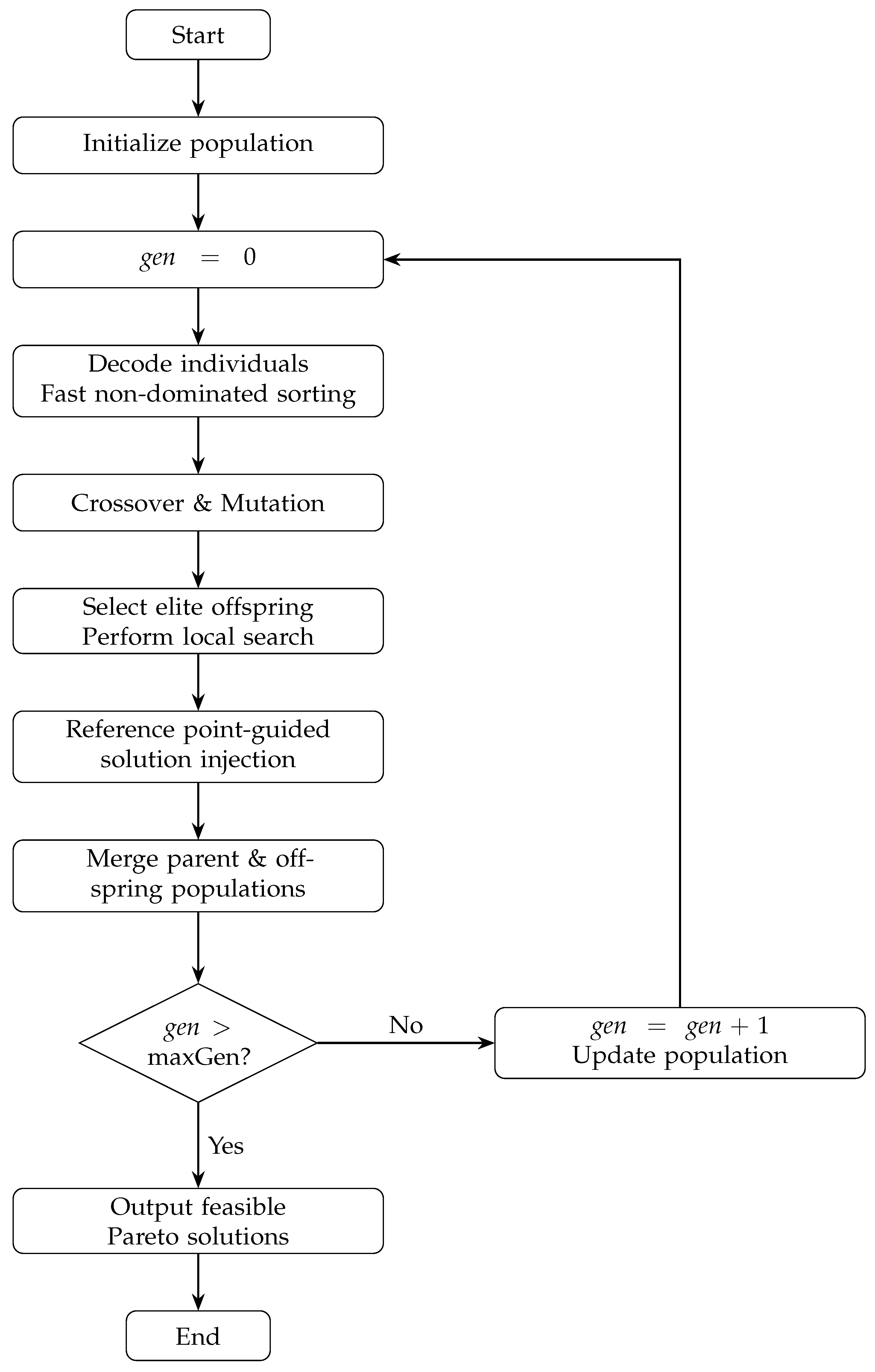
Figure 1 shows the flow of the algorithm.

5.1. Chromosome Encoding and Decoding

In the integrated scheduling problem, production and transportation operations are highly coupled in both time and space. To achieve joint optimization, the chromosome in this algorithm adopts a three-segment encoding scheme:

$$\mathrm{Chrom}=\left[\pi \mid \mathrm{a}\mid \rho \right].$$

where $\pi$ is the production sequence gene, $\mathrm{a}$ is the transport resource assignment gene, and $\rho$ is the transport task priority gene.

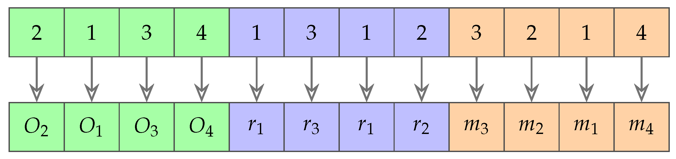
Figure 2 illustrates the three-segment chromosome encoding. The first segment, denoted by $\pi$, represents the production sequence by listing operation IDs in the order of scheduling priority. The second segment, denoted by $\mathrm{a}$, assigns material handling resources, where each gene specifies the resource selected for a transport task $m\in \mathcal{M}$. The third segment, denoted by $\rho$, determines transport priorities by listing transport task IDs. Compared with a single-layer representation, this integrated encoding jointly captures production sequencing, resource assignment, and transport prioritization within one decoding framework.

Figure 1. IMNSGA-II framework flowchart.

Figure 1. IMNSGA-II framework flowchart.

Figure 2. Illustration of the three-segment chromosome.

Figure 2. Illustration of the three-segment chromosome.

During evaluation, the discrete event-driven decoder tracks the real-time status of production resources, material handling resources, buffer occupancy, and shared safety zones. It updates the key time variables accordingly, including the operation start time $S_i$, completion time $C_i$, resource release time $F_i$, transport start time $T_m^S$, and transport finish time $T_m^F$. After decoding, the objective vector for a solution x is evaluated according to the following dominance rule:

$$x\prec y\iff \left\{\begin{array}{c}P\left(x\right)=0,P\left(y\right)>0,\hfill \\ P\left(x\right)>0,P\left(y\right)>0,P\left(x\right)<P\left(y\right),\hfill \\ P\left(x\right)=P\left(y\right)=0,\mathbf{f}\left(x\right){\prec }_{\mathrm{P}}\mathbf{f}\left(y\right).\hfill \end{array}\right.$$

(37)

Here, $f_1\left(x\right)$ denotes the makespan, $f_2\left(x\right)$ denotes the total empty travel time, and $\mathbf{f}\left(x\right)=(f_1\left(x\right),f_2\left(x\right))$ denotes the bi-objective vector; boldface is used only for vector quantities in the equations. To handle hard constraints such as synchronous assembly and buffer blocking, a penalty function $P\left(x\right)\ge 0$ is introduced. This function quantifies violations of precedence constraints, synchronous assembly requirements, resource-capacity conflicts, transport scheduling conflicts, service-area mismatches, safety-zone overlaps, and buffer limits. Every time there is a violation of a constraint, the function imposes a large penalty value. Under this rule, feasible solutions always dominate infeasible ones; among infeasible solutions, those with smaller penalties are preferred; and among feasible solutions, Pareto dominance is used. This does not mean that the hard constraints in MILP are relaxed into soft constraints. On the contrary, the algorithm follows a hierarchical feasibility handling mechanism. First, the repair procedure restores chromosome-level consistency after genetic mutation. Then, the event-driven decoder checks the feasibility of time and resources by explicitly simulating situations such as machine occupation, transportation execution, buffer occupation, blocking release, and safe-zone exclusion. Only when there are still infeasible situations after decoding will a huge penalty term be assigned to eliminate the individual in environmental selection. Therefore, the penalty term mainly serves as a sorting mechanism for partially infeasible individuals during the search process, while the actual hard constraints are enforced as much as possible through repair and decoding. To reduce computational cost during iterative evolution, each individual stores its evaluation metrics, including objective values, penalty scores, non-dominated rank, and crowding distance.

Based on the three-segment representation, IMNSGA-II adopts specialized genetic operators:

• Crossover: With crossover probability $P_c$, partial mapping crossover (PMX) is applied to the $\pi$ part (production sequence) in order to preserve the relative priority of operations within the same part. For the $\mathrm{a}$ and $\rho$ parts, position-based crossover (POX) and two-point crossover (TPX) are applied, respectively. This combination promotes effective gene recombination while preserving critical transport resource assignments.
• Mutation: Multi-neighborhood mutation is applied with probabilities $P_m^{\pi }$, $P_m^{\mathrm{a}}$, and $P_m^{\rho }$ for the $\pi$, $\mathrm{a}$, and $\rho$ parts, respectively. The $\pi$ part uses insertion and swap mutations; the $\mathrm{a}$ part performs single-point or multi-point reassignment within available material handling resources; and the $\rho$ part uses reversal or adjacent swap operations.

Because the integrated scheduling problem is highly constrained, conventional crossover and mutation operators may generate infeasible chromosomes. Therefore, each offspring undergoes a repair process before decoding to remove redundant transport decisions and restore consistency among production priorities, transport assignments, and transport priorities.

5.2. Local Search

To enhance the algorithm’s local exploitation capability for elite solutions, this paper embeds a local search mechanism based on Variable Neighborhood Search (VNS) and a Simulated Annealing (SA) acceptance criterion into NSGA-II. In the algorithm configuration, the local-search stage is controlled by the trigger probability $P_{\mathrm{LS}}$, elite ratio ${\rho }_{\mathrm{LS}}$, local-search budget $B_{\mathrm{LS}}$, and retained elite size $N_{\mathrm{elite}}$.

The local search operates directly on the aforementioned three-segment encoding, perturbing and improving the current individual through various complementary neighborhoods. After each perturbation or small-step search, a repair procedure is invoked to restore encoding consistency and ensure subsequent decoding feasibility.

Unlike traditional local searches that only fine-tune a single encoding segment, this paper adopts four types of neighborhood structures:

$$\mathcal{N}=\left\{{\mathcal{N}}_1^{\pi },{\mathcal{N}}_2^{\mathrm{a}},{\mathcal{N}}_3^{\rho },{\mathcal{N}}_4^{\mathrm{mix}}\right\},$$

corresponding to the production sequence neighborhood, resource assignment neighborhood, transport priority neighborhood, and mixed neighborhood, respectively. The first three types of neighborhoods conduct targeted searches on a specific encoding segment, while the mixed neighborhood randomly selects one of the three types of operations ($\pi /\mathrm{a}/\rho$) to execute at each step, thereby striking a balance between local intensification and cross-segment coordination.

• In ${\mathcal{N}}_1^{\pi }$, a swap operation is executed with a higher probability; otherwise, an insert/shift operation is performed. Utilizing a probability of 0.7 for the swap operation biases the algorithm toward fine-grained search while still retaining structural rearrangement capabilities to escape local optima.
• In ${\mathcal{N}}_2^{\mathrm{a}}$, a handling task is randomly selected, and a resource is resampled from its set of available resources.
• In ${\mathcal{N}}_3^{\rho }$, two positions are randomly selected, and their priorities are swapped.
• In ${\mathcal{N}}_4^{\mathrm{mix}}$, one of the three operations ($\pi /\mathrm{a}/\rho$) is randomly selected at each step to execute the corresponding variation.
• During the inner local fine-tuning phase, one of the three basic operations ($\pi /\mathrm{a}/\rho$) is also randomly selected at each step, and only candidate solutions that improve the current local optimum are retained.

Since neighborhood variations may lead to encoding inconsistencies, invalid resource assignments, or decoding conflicts, this paper executes a repair operation after each perturbation:

$$x^{\prime }\leftarrow \mathrm{repair}\left(x^{\prime }\right).$$

The repair procedure is primarily used to restore the consistency and decodability of the chromosome, which includes: ensuring that the lengths of the three encoding segments match the task set; guaranteeing that the resource assignments in the $\mathrm{a}$ segment satisfy service area and compatibility constraints; eliminating duplicate or illegal encoding elements; and restoring the consistent correspondence between the encoding segments. Once the repair is completed, the event-driven decoder is employed to recalculate the performance metrics of the candidate solution, and the decision to accept the candidate solution is made by combining the Pareto dominance relation with the simulated annealing acceptance criterion. It is worth noting that the repair procedure is only used to restore the consistency and decodability of the encoding, while blocking diffusion is handled by the event-driven decoder. Specifically, when an operation finishes processing but its downstream buffer is full, the allocated processing resources are not yet available, or the next stage cannot receive the component, the job remains on the current machine, and the release time of that machine is delayed until the actual pickup time. This delayed release may, in turn, postpone subsequent operations on the same machine and propagate congestion to upstream stages. The decoder updates these interactions through event sequences, thereby capturing the propagation effect of blocking under limited buffers and coupled transportation resources. After this dynamic propagation is completed, any remaining infeasibilities are quantified by a penalty function. The specific procedure is illustrated in Algorithm 1.

Algorithm 1: VNS–SA Local Search Based on Four Neighborhood Types

5.3. SA Acceptance Criterion

To enhance the algorithm’s ability to escape local optima during local search, a simulated annealing criterion is adopted to accept worse solutions with a certain probability. The initial temperature is set as

$$T_0=max\left\{T_{min},\varphi \right\},$$

(38)

where $\varphi$ is the initial temperature factor, $\eta$ is the cooling rate, and $T_{min}$ is the minimum temperature. In the experiments, $\varphi =0.10$, $\eta =0.995$, and $T_{min}={10}^{-6}$.

Let ${\left[u\right]}_{+}=max(u,0)$ and let $\epsilon >0$ be a small positive constant. If $x^{\prime }\prec x^{\mathrm{cur}}$, the candidate solution is accepted directly. Otherwise, the degree of deterioration of $x^{\prime }$ relative to $x^{\mathrm{cur}}$ is defined as

$${\Delta }_{\mathrm{SA}}\left(x^{\prime },x^{\mathrm{cur}}\right)={\left[{\displaystyle \frac{C_{max}\left(x^{\prime }\right)-C_{max}\left(x^{\mathrm{cur}}\right)}{C_{max}\left(x^{\mathrm{cur}}\right)+\epsilon }}\right]}_{+}+{\left[{\displaystyle \frac{E\left(x^{\prime }\right)-E\left(x^{\mathrm{cur}}\right)}{E\left(x^{\mathrm{cur}}\right)+\epsilon }}\right]}_{+}+{\left[P\left(x^{\prime }\right)-P\left(x^{\mathrm{cur}}\right)\right]}_{+}.$$

(39)

Accordingly, when $x^{\prime }$ does not dominate $x^{\mathrm{cur}}$, the acceptance probability is

$$Pr\left(\mathrm{accept}{x}^{\prime }\right)=\left\{\begin{array}{cc}1,\hfill & {\Delta }_{\mathrm{SA}}\le 0,\hfill \\ exp\left(-{\Delta }_{\mathrm{SA}}/T\right),\hfill & {\Delta }_{\mathrm{SA}}>0.\hfill \end{array}\right.$$

(40)

The temperature is updated according to a geometric cooling schedule:

$$T\leftarrow max\left(T_{min},\eta T\right).$$

(41)

If $x^{\prime }$ is accepted, then $x^{\mathrm{cur}}\leftarrow x^{\prime }$ and the neighborhood index is reset to the first neighborhood. Otherwise, the search proceeds to the next neighborhood in VNS. This rule applies both when $x^{\prime }$ is dominated by $x^{\mathrm{cur}}$ and when the two solutions are mutually non-dominated.

5.4. Reference-Point-Guided Injection Mechanism

To improve the coverage of different preference regions on the Pareto front, a reference-point-guided injection mechanism is introduced after the elite local-search stage. To avoid confusion with the handling-resource set $\mathcal{R}$ in the mathematical formulation, the set of reference-point vectors is denoted by

$$\Omega =\left\{{\mathbf{r}}^1,{\mathbf{r}}^2,\dots ,{\mathbf{r}}^L\right\}.$$

(42)

In the normalized bi-objective space, the ℓ-th reference-point vector is defined as

$${\mathbf{r}}^{\ell }=\left({\lambda }^{\ell },1-{\lambda }^{\ell }\right),{\lambda }^{\ell }={\displaystyle \frac{\ell -1}{L-1}},\ell =1,\dots ,L,$$

(43)

where $L=5$ in the experiments. It is selected based on previous experimental experience, aiming to balance the computational cost of the algorithm and the coverage breadth of the Pareto frontier. Smaller ${\lambda }^{\ell }$ emphasizes the $C_{max}$-oriented region, larger ${\lambda }^{\ell }$ emphasizes the E-oriented region, and intermediate reference points correspond to more balanced trade-off regions.

Let the current candidate pool be

$${\mathcal{C}}_t={\mathrm{Pop}}_t\cup {\mathrm{Off}}_t.$$

For each $x\in {\mathcal{C}}_t$, the normalized objectives are computed as

$$\begin{array}{cc}\hfill {\widehat{C}}_{max}\left(x\right)& ={\displaystyle \frac{C_{max}\left(x\right)-C_{max}^{min}}{C_{max}^{max}-C_{max}^{min}+\epsilon }},\hfill \end{array}$$

(44)

$$\begin{array}{cc}\hfill \widehat{E}\left(x\right)& ={\displaystyle \frac{E\left(x\right)-E^{min}}{E^{max}-E^{min}+\epsilon }},\hfill \end{array}$$

(45)

where $C_{max}^{min}$, $C_{max}^{max}$, $E^{min}$, and $E^{max}$ are computed from ${\mathcal{C}}_t$. The distance between a candidate solution x and a reference point ${\mathbf{r}}^{\ell }$ is then defined as

$$D\left(x,{\mathbf{r}}^{\ell }\right)=\sqrt{{\left({\widehat{C}}_{max}\left(x\right)-{\lambda }^{\ell }\right)}^2+{\left(\widehat{E}\left(x\right)-\left(1-{\lambda }^{\ell }\right)\right)}^2}.$$

(46)

For each reference point ${\mathbf{r}}^{\ell }$, a seed solution $x^{\ell }$ is selected from ${\mathcal{C}}_t$ according to the following priority rules: feasible solutions are preferred to infeasible ones; among solutions with the same feasibility status, the one with the smaller distance $D(x,{\mathbf{r}}^{\ell })$ is preferred; ties are then broken by lower non-dominated rank and larger crowding distance.

Each seed solution is further refined once by a directional memetic local search to generate an injected candidate ${\tilde{x}}^{\ell }$. Here, “directional” means that the same memetic local-search framework is biased toward the preference region represented by ${\mathbf{r}}^{\ell }$: for endpoint reference points, candidate solutions in the local-search step are compared primarily according to the corresponding single objective ($C_{max}$ or E), whereas for intermediate reference points the original Pareto-based comparison is retained. This injection step is triggered once in each generation after the elite local-search stage. After duplicate removal, each ${\tilde{x}}^{\ell }$ is appended to the offspring pool ${\mathrm{Off}}_t$ rather than directly replacing any existing individual; the final survivors are determined only in the subsequent environmental selection on ${\mathrm{Pop}}_t\cup {\mathrm{Off}}_t$.

In summary, the framework of IMNSGA-II is shown in Algorithm 2. It should be noted that IMNSGA-II is implemented in a serial manner in this study. Its ability to handle medium- and large-scale instances mainly comes from the problem-specific encoding, decoding/repair strategy, elite-guided local search, and reference-point-guided injection mechanism, which together improve search efficiency under a fixed computational budget. Nevertheless, due to its population-based structure, IMNSGA-II is naturally compatible with future parallelization. In particular, GPU- or MPI-based implementations for fitness evaluation, offspring generation, and partial ranking/diversity operations may further improve its efficiency on larger-scale instances, which will be an important direction for future research.

Algorithm 2: Main Framework of the Proposed IMNSGA-II

6. Experimental Results and Analysis

The algorithms were implemented in Java 21 and executed on a PC equipped with an Intel(R) Core(TM) i7-10700F CPU @ 2.90 GHz and 16 GB of RAM. The basic test instances were adopted from the benchmark instances reported in [21]. To make them consistent with the problem studied in this paper, the instances were extended by incorporating finite buffers, service-area restrictions, empty travel times, and safety-zone mutual exclusion.

The 20 benchmark instances are denoted by I01–I20. Specifically, I01–I10 correspond to Yang’s small-scale MFJSTA01–10 family, whereas I11–I20 correspond to the medium- and large-scale MKTA01–10 family. The inherited benchmark data include the original processing-stage data, product–job partitions, and assembly-time vectors, while the effective difficulty further increases with the added transportation–assembly coupling factors, namely finite buffers, service-area restrictions, empty travel, and safety-zone mutual exclusions. Appendix A now summarizes the benchmark mapping, the added extension parameters, and the inherited structural information of each instance, and Appendix B reports the detailed settings of the comparative baseline algorithms.

6.1. Parameter Settings

The experiments include 20 instances (I01–I20) and use 10 random seeds. Since the time consumed by a single iteration differs substantially across algorithms, all subsequent experiments use a unified time limit instead of a unified number of generations for fairness. The global time limit is set to 50,000 ms. The parameter settings of IMNSGA-II are reported in

Table 2. Parameter settings of IMNSGA-II.

Symbol	Description	Value
$N_{\mathrm{pop}}$	Population size	80
$G_{max}$	Maximum number of generations	100,000
$P_c$	Crossover probability	0.85
$P_m^{\pi }$	Mutation probability of the production segment	0.10
$P_m^{\mathrm{a}}$	Mutation probability of the assignment segment	0.08
$P_m^{\rho }$	Mutation probability of the transport-priority segment	0.10
$N_{\mathrm{elite}}$	Number of elite individuals retained	8
$k_{\mathrm{tour}}$	Tournament size	2
$P_{\mathrm{LS}}$	Trigger probability of local search	0.30
$B_{\mathrm{LS}}$	Local-search budget	40
${\rho }_{\mathrm{LS}}$	Elite ratio for local search	0.30
$k_{max}$	Maximum VNS neighborhood level	4
$\varphi$	Initial temperature factor	0.10
$T_{min}$	Minimum temperature	${10}^{-6}$
$\eta$	SA cooling rate	0.995
L	Number of reference points	5

. The performance metrics reported below are averages over 10 random seeds. Both the ablation experiments and the comparative experiments use IGD (Inverted Generational Distance) and HV (Hypervolume) to evaluate the quality of the obtained feasible Pareto fronts. Since the true Pareto-optimal front is unknown for these instances, an approximate reference front is constructed for each instance by pooling all feasible solutions obtained by all compared algorithms over all runs and extracting the non-dominated subset. Both IGD and HV are computed in the normalized objective space, where each objective is scaled by min–max normalization using the minimum and maximum values of the corresponding approximate reference front. For HV calculation, the reference-point vector is set to a point that is 10% worse than the worst value of the approximate reference front in each objective, i.e.,

$${\mathbf{r}}^{\mathrm{HV}}=\left(C_{max}^{max}+0.1\left(C_{max}^{max}-C_{max}^{min}\right),E^{max}+0.1\left(E^{max}-E^{min}\right)\right).$$

If the range of one objective is zero, a small positive padding is used to avoid degeneration. The reported HV values are further normalized by the area of the corresponding reference rectangle, so that larger HV indicates better overall front quality, whereas smaller IGD indicates better proximity to the reference front. Note that this HV reference point is used only for performance evaluation and is different from the reference points adopted in the reference-point-guided injection mechanism. The standard definitions of IGD and HV follow [33].

The detailed parameter settings and shared decoding assumptions of the representative comparative baselines are reported in Appendix B.

6.2. Taguchi Parameter Calibration

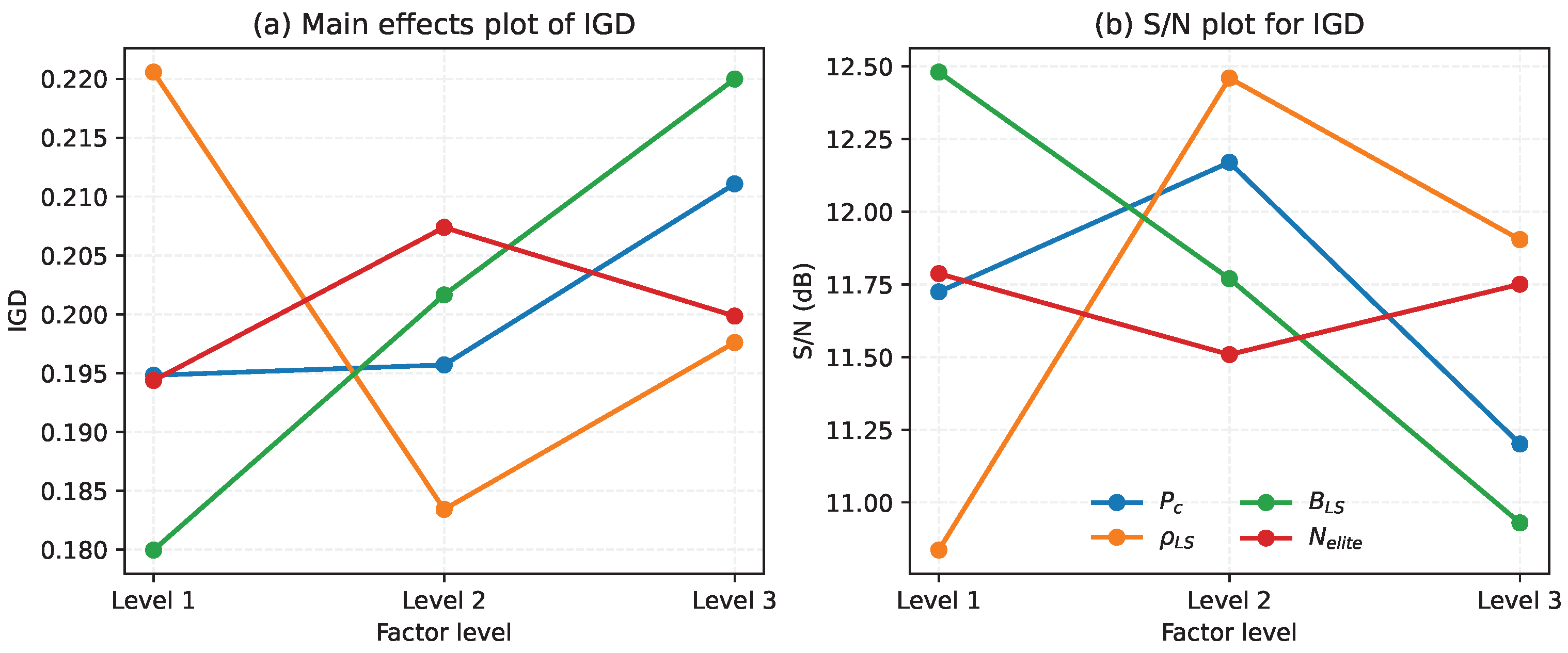
To provide explicit calibration evidence for the most disputed parameters, a supplementary Taguchi $L_9\left(3^4\right)$ experiment was conducted for $P_c$, ${\rho }_{\mathrm{LS}}$, $B_{\mathrm{LS}}$, and $N_{\mathrm{elite}}$, with the corresponding levels $\{0.75,0.85,0.95\}$, $\{0.20,0.30,0.40\}$, $\{40,80,120\}$, and $\{4,6,8\}$. The remaining parameters were fixed at the values in Table 2. Four representative instances (I04, I08, I14, and I20) and five random seeds were used for each orthogonal-design row under the same 50 s time limit as in the main experiments.

Table 3. Summary of the Taguchi L9($3^4$) parameter calibration study.

Row	${\mathit{P}}_{\mathit{c}}$	${\mathit{\rho }}_{\mathbf{LS}}$	${\mathit{B}}_{\mathbf{LS}}$	${\mathit{N}}_{\mathbf{elite}}$	Mean HV	Mean IGD	Mean Time (s)	S/N (IGD)
R1	0.75	0.20	40	4	0.3922	0.1881	50.88	11.6286
R2	0.75	0.30	80	6	0.3440	0.1857	53.50	12.4088
R3	0.75	0.40	120	8	0.2946	0.2107	52.41	11.2183
R4	0.85	0.20	80	8	0.3291	0.2162	52.50	11.3804
R5	0.85	0.30	120	4	0.2978	0.1919	52.97	12.1694
R6	0.85	0.40	40	6	0.3729	0.1791	51.94	13.1353
R7	0.95	0.20	120	6	0.2765	0.2574	54.28	9.7487
R8	0.95	0.30	40	8	0.3779	0.1727	50.79	12.8258
R9	0.95	0.40	80	4	0.3209	0.2031	52.69	11.5866

reports the row-level mean HV, mean IGD, mean runtime, and the corresponding IGD-based S/N ratio. Figure 3 shows the factor-level main effects of IGD and the corresponding S/N ratio. Among the nine orthogonal combinations, R8 ($P_c=0.95$, ${\rho }_{\mathrm{LS}}=0.30$, $B_{\mathrm{LS}}=40$, and $N_{\mathrm{elite}}=8$) achieved the lowest mean IGD of 0.1727, whereas R1 attained the highest mean HV of 0.3922. The factor-level analysis indicates that ${\rho }_{\mathrm{LS}}=0.30$ and $B_{\mathrm{LS}}=40$ are consistently preferred by both mean IGD and S/N. For $P_c$, the mean IGD values at 0.75 and 0.85 are very close (0.1948 and 0.1957), while the S/N ratio slightly favors 0.85, indicating better robustness. For $N_{\mathrm{elite}}$, the smallest mean IGD and the highest S/N are both obtained at 4, although the difference from 8 is small. Overall, the Taguchi experiment confirms the robustness of a moderate crossover probability and a local-search elite ratio of 0.30, while also showing diminishing returns when overly large local-search budgets or elite-retention sizes are used. This subsection is therefore included as a supplementary reproducibility check for the benchmark configuration in Table 2. The parameter settings in Table 2 have been modified to $P_c=0.85$, ${\rho }_{\mathrm{LS}}=0.30$, $B_{\mathrm{LS}}=40$, and $N_{\mathrm{elite}}=8$ based on the Taguchi experiment results.

6.3. Small-Scale Exact Solving

To verify the feasibility and solvability of the mathematical model, Gurobi was first used to solve a weighted-sum MIP on the small-scale instances I01–I12, with a 50 s time limit. To better characterize the difficulty of the borderline cases, I05–I08 were additionally rerun with a 300 s time limit.

Table 4. Summary of Gurobi results on small-scale instances.

Instance	${\mathit{C}}_{max}$	E	Status	Time (s)	MIP Gap (%)
I01	38.000	13.000	Optimal	0.262	0.000
I02	43.000	13.000	Optimal	0.337	0.000
I03	37.000	13.000	Optimal	0.102	0.000
I04	39.200	12.100	Optimal	0.140	0.000
I05	67.400	38.500	Time limit	300.467	22.024
I06	67.000	40.700	Time limit	300.445	16.609
I07	61.800	41.800	Time limit	300.573	9.235
I08	58.800	48.000	Time limit	300.862	7.719
I09	–	–	No solution	50.374	–
I10	–	–	No solution	50.218	–
I11	–	–	No solution	50.290	–
I12	–	–	No solution	50.173	–

Note: I05–I08 were rerun with a 300 s time limit to report the remaining Gurobi-reported relative MIP gaps for the weighted-sum objective at termination. I01–I04 and I09–I12 retain the original 50 s setting.

summarizes $C_{max}$, E, solution status, runtime, and the corresponding Gurobi-reported relative MIP gap when available. The results show that optimal solutions can be obtained within 50 s for I01–I04. For I05–I08, even after extending the time limit to 300 s, the remaining Gurobi-reported relative MIP gaps are still 22.024%, 16.609%, 9.235%, and 7.719%, respectively, indicating that Gurobi can find incumbents but still cannot certify optimality at this relatively small scale. By contrast, no feasible solution is returned for I09–I12 within the original 50 s limit. These results confirm that the proposed model can accurately characterize the problem while also showing that the computational burden of exact optimization increases rapidly with instance size. This further justifies the use of IMNSGA-II for medium- and large-scale instances.

Because exact Pareto fronts are additionally available for I01–I04, IMNSGA-II can also be evaluated directly against the exact fronts instead of a pooled heuristic reference set.

Table 5. Gap of IMNSGA-II to the exact Pareto front on instances I01–I04.

Instance	IGD	Coverage
I01	0.447	1.000
I02	0.659	1.000
I03	0.585	2.000
I04	0.614	1.000
Mean	0.591	1.250

reports the resulting IGD and coverage values, where lower IGD and higher coverage are preferred. The results show that IMNSGA-II remains close to the exact fronts on all four instances, although few exact Pareto points are recovered exactly within the current heuristic time budget.

6.4. Decoupling Experiments

To verify the necessity of coordinated optimization among production, transport, and assembly decisions, decoupling experiments were further conducted. Unlike the proposed method, which jointly optimizes $[\pi \mid \mathrm{a}\mid \rho ]$ within a unified individual, the decoupled baselines handle production sequencing and transport decisions in separate stages: a production plan is determined first, after which transport and assembly decisions are generated by rules. IMNSGA-II exhibits a clear advantage in the decoupling experiments, achieving the best values for both $C_{max}$ and E on all 20 instances.

Table 6. Instance-level comparison of $C_{max}$ and E in the decoupling experiments.

Instance	Decoupled-Baseline		IMNSGA-II
	${\mathit{C}}_{max}$	$\mathit{E}$	${\mathit{C}}_{max}$	$\mathit{E}$
I01	–	–	47.000	12.000
I02	48.000	13.000	48.000	13.000
I03	–	–	44.000	14.000
I04	–	–	46.700	13.200
I05	87.200	49.500	70.900	37.400
I06	85.900	42.900	75.767	35.933
I07	81.500	42.900	71.300	39.600
I08	78.400	43.200	68.600	38.400
I09	122.100	81.400	104.000	61.600
I10	109.700	72.600	97.933	63.067
I11	101.700	77.000	93.500	65.267
I12	109.800	79.200	97.067	69.600
I13	158.200	110.000	133.600	88.367
I14	153.100	106.700	132.367	88.367
I15	131.100	104.500	121.667	93.867
I16	136.600	110.400	121.933	102.400
I17	177.800	134.200	161.267	117.333
I18	183.900	137.500	174.400	114.767
I19	159.600	133.100	147.733	124.300
I20	179.000	145.200	152.267	135.600

Note: ‘–’ indicates that the corresponding method failed to generate a feasible solution. Bold indicates the better value in each row; ties are shown in bold for all tied entries.

reports the instance-level comparison of $C_{max}$ and E. Over the instances for which both IMNSGA-II and Decoupled-Baseline return feasible solutions, IMNSGA-II reduces $C_{max}$ by approximately 10.16% and E by approximately 12.33%.

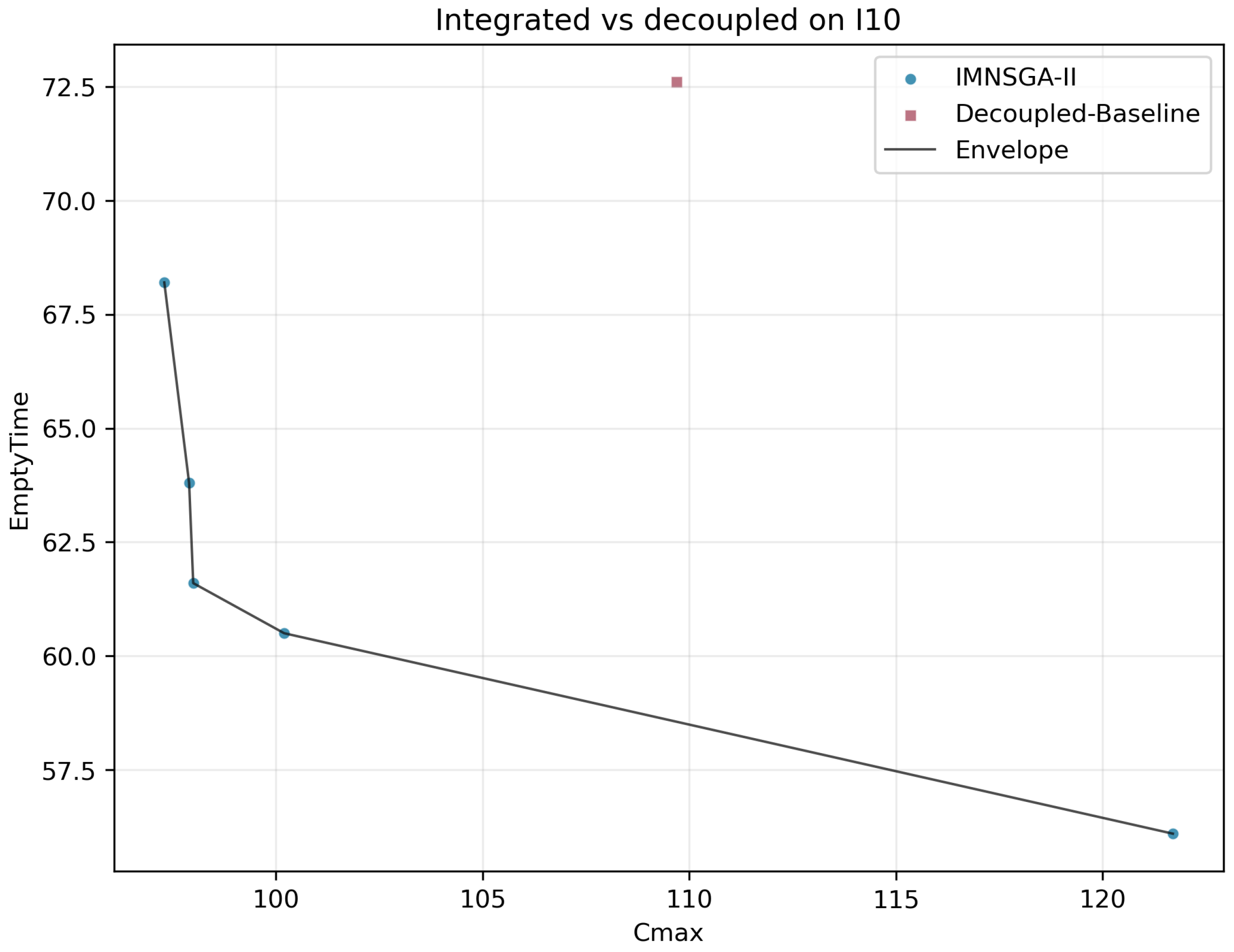
Figure 4 further shows that IMNSGA-II dominates the decoupled baselines in both objectives over the displayed solutions.

6.5. Ablation Experiments

To evaluate the effectiveness of the improvement modules embedded in IMNSGA-II, the proposed algorithm is compared, under the same encoding scheme, decoder, population size, stopping criterion, and parameter budget, with three variants: IMNSGA-II-w/oLS (without local search), IMNSGA-II-w/oSA (without the SA acceptance criterion), and IMNSGA-II-w/oTN (without tailored neighborhoods and using a simple local search instead).

Table 7 presents the HV and IGD results for all instances. IMNSGA-II performs best on both front-quality indicators, achieving the best HV on 18 out of 20 instances and the best IGD on 19 out of 20 instances.

Overall, the ablation results reveal a consistent pattern across both HV and IGD: removing any of the three improvement components leads to a noticeable deterioration in front quality. In particular, the full IMNSGA-II attains the best mean HV and IGD values among all variants, indicating that the proposed local search framework, the SA-based acceptance criterion, and the tailored neighborhood structures contribute complementarily rather than independently. This cross-metric consistency suggests that the performance gain of IMNSGA-II is not limited to either convergence or diversity alone, but arises from a more balanced improvement of the overall Pareto front quality.

Table 7. Instance-level comparison of HV and IGD in the ablation experiments.

Instance	IMNSGA-II w/oLS		IMNSGA-II w/oSA		IMNSGA-II w/oTN		IMNSGA-II
	HV	IGD	HV	IGD	HV	IGD	HV	IGD
I01	0.309	4.123	0.309	4.123	0.309	4.123	0.586	4.123
I02	0.041	0.707	0.206	0.707	0.138	0.707	0.446	0.707
I03	0.876	1.302	0.876	1.302	0.876	1.302	0.967	0.604
I04	0.258	2.493	0.176	2.493	0.228	2.493	0.528	0.707
I05	0.091	0.856	0.258	0.856	0.551	0.856	1.312	0.291
I06	0.714	4.357	0.112	4.357	0.425	4.357	1.331	3.992
I07	0.213	0.644	0.218	0.644	0.452	0.644	0.655	0.291
I08	0.478	0.728	0.421	0.728	0.214	0.728	0.582	0.121
I09	0.091	0.846	0.152	0.846	0.225	0.846	0.383	0.248
I10	0.581	0.743	0.152	0.743	0.513	0.743	0.598	0.267
I11	0.210	0.615	0.279	0.615	0.119	0.615	0.791	0.327
I12	0.189	0.662	0.144	0.549	0.142	0.549	0.483	0.190
I13	0.310	0.775	0.156	0.775	0.315	0.775	0.573	0.375
I14	0.325	0.763	0.091	0.763	0.091	0.763	1.073	0.374
I15	0.210	1.097	0.301	1.097	0.278	1.097	0.462	0.275
I16	0.266	0.233	0.122	0.362	0.122	0.362	0.378	0.277
I17	0.172	3.788	0.983	3.788	0.517	3.788	0.319	0.613
I18	0.091	0.889	0.255	0.889	0.091	0.889	0.662	0.272
I19	0.189	0.962	0.526	0.962	0.428	0.962	0.617	0.333
I20	0.361	0.314	0.308	0.360	0.295	0.369	0.299	0.249
Mean	0.299	1.345	0.302	1.348	0.316	1.348	0.652	0.732
Average processing time (s)	49.627		50.483		50.308		50.291

Note: For HV, larger values are better; for IGD, smaller values are better. Bold indicates the best value in each row for the corresponding metric, and ties are shown in bold for all tied entries.

Table 7. Instance-level comparison of HV and IGD in the ablation experiments.

Instance	IMNSGA-II w/oLS		IMNSGA-II w/oSA		IMNSGA-II w/oTN		IMNSGA-II
	HV	IGD	HV	IGD	HV	IGD	HV	IGD
I01	0.309	4.123	0.309	4.123	0.309	4.123	0.586	4.123
I02	0.041	0.707	0.206	0.707	0.138	0.707	0.446	0.707
I03	0.876	1.302	0.876	1.302	0.876	1.302	0.967	0.604
I04	0.258	2.493	0.176	2.493	0.228	2.493	0.528	0.707
I05	0.091	0.856	0.258	0.856	0.551	0.856	1.312	0.291
I06	0.714	4.357	0.112	4.357	0.425	4.357	1.331	3.992
I07	0.213	0.644	0.218	0.644	0.452	0.644	0.655	0.291
I08	0.478	0.728	0.421	0.728	0.214	0.728	0.582	0.121
I09	0.091	0.846	0.152	0.846	0.225	0.846	0.383	0.248
I10	0.581	0.743	0.152	0.743	0.513	0.743	0.598	0.267
I11	0.210	0.615	0.279	0.615	0.119	0.615	0.791	0.327
I12	0.189	0.662	0.144	0.549	0.142	0.549	0.483	0.190
I13	0.310	0.775	0.156	0.775	0.315	0.775	0.573	0.375
I14	0.325	0.763	0.091	0.763	0.091	0.763	1.073	0.374
I15	0.210	1.097	0.301	1.097	0.278	1.097	0.462	0.275
I16	0.266	0.233	0.122	0.362	0.122	0.362	0.378	0.277
I17	0.172	3.788	0.983	3.788	0.517	3.788	0.319	0.613
I18	0.091	0.889	0.255	0.889	0.091	0.889	0.662	0.272
I19	0.189	0.962	0.526	0.962	0.428	0.962	0.617	0.333
I20	0.361	0.314	0.308	0.360	0.295	0.369	0.299	0.249
Mean	0.299	1.345	0.302	1.348	0.316	1.348	0.652	0.732
Average processing time (s)	49.627		50.483		50.308		50.291

Note: For HV, larger values are better; for IGD, smaller values are better. Bold indicates the best value in each row for the corresponding metric, and ties are shown in bold for all tied entries.

6.6. Comparative Experiments

To verify the effectiveness of IMNSGA-II, it is compared with four representative comparative baselines: an NSGA-II baseline [34], ALNS [35], MOGWO [36], and MOWOA [37]. These baselines were selected because they cover population-based evolutionary search, adaptive neighborhood search, and two widely used swarm-based multi-objective frameworks. Recent hybrid shop-scheduling algorithms often embed highly problem-specific local search operators tailored to simpler blocking-free or transport-free settings. Reimplementing such operators for the present problem, which couples finite buffers, synchronous assembly, service-area restrictions, and shared safety zones, would require substantial redesign of the decoding framework and would confound a like-for-like comparison. Therefore, all compared algorithms are evaluated under the same three-segment encoding/decoding framework, the same feasibility-handling mechanism, and the same 50 s wall-clock budget. More complex hybrid algorithms or GPU/MPI-accelerated implementations may provide additional insight in future studies, but they are beyond the scope of the current revision because they require extra problem-specific modules or parallel hardware settings. The detailed parameter settings of the comparative baselines are provided in Appendix B. The performance evaluation follows the normalized IGD/HV protocol defined above. The results are reported in

Table 8. Instance-level comparison of HV and IGD in the comparative experiments.

Instance	IMNSGA-II		NSGA-II		ALNS		MOGWO		MOWOA
	HV	IGD	HV	IGD	HV	IGD	HV	IGD	HV	IGD
I01	1.021	1.732	0.214	0.920	0.983	0.782	0.539	1.609	0.320	1.688
I02	0.376	0.153	0.091	0.707	0.174	0.291	0.174	0.604	0.226	0.854
I03	0.336	0.111	0.119	0.451	0.311	0.327	0.327	0.111	0.321	0.241
I04	0.874	0.412	0.715	2.493	0.118	0.707	0.080	1.180	0.124	1.478
I05	1.367	0.233	0.142	0.856	1.546	0.991	1.394	2.573	0.659	2.364
I06	4.028	0.707	0.801	4.357	4.050	1.574	0.726	2.853	0.891	2.531
I07	0.714	0.147	0.217	0.644	0.437	0.214	0.183	0.754	0.207	0.500
I08	0.675	0.097	0.102	0.728	0.393	0.296	0.126	0.605	0.084	0.662
I09	0.496	0.202	0.355	0.846	0.275	0.326	0.039	1.182	0.102	1.102
I10	0.658	0.193	0.426	0.743	0.406	0.342	0.250	0.769	0.224	0.682
I11	0.910	0.196	0.381	0.615	0.381	0.312	0.077	2.110	0.039	1.096
I12	0.636	0.096	0.446	0.519	0.230	0.414	0.067	0.763	0.059	0.754
I13	0.707	0.311	0.501	0.775	0.247	0.503	0.219	0.983	0.127	1.046
I14	1.279	0.316	0.229	0.763	0.620	0.431	0.435	0.918	0.145	0.807
I15	0.591	0.143	0.238	1.097	0.243	0.422	0.094	0.875	0.201	0.610
I16	0.389	0.198	0.296	0.220	0.171	0.382	0.034	0.855	0.069	0.856
I17	0.862	0.269	0.335	3.788	0.149	0.813	0.318	2.255	0.707	1.986
I18	0.709	0.241	0.105	0.889	0.564	0.375	0.249	0.709	0.106	0.742
I19	0.413	0.151	0.230	0.962	0.115	0.451	0.009	1.097	0.212	0.663
I20	0.372	0.191	0.372	0.309	0.222	0.362	0.075	0.693	0.115	0.613
Average	0.871	0.305	0.316	1.134	0.582	0.516	0.271	1.175	0.247	1.064
Average processing time (s)	50.312		50.849		47.867		49.891		49.302

Note: For HV, larger values are better; for IGD, smaller values are better. Bold indicates the best value in each row for the corresponding metric, and ties are shown in bold for all tied entries.

, where the best values are highlighted in bold. IMNSGA-II achieves the best HV on 18 out of 20 instances and the best IGD on 19 out of 20 instances, while also obtaining the best average values for both HV and IGD. Table 8 additionally reports the average processing time (PT, s) of the comparative baselines. Under the same 50 s wall-clock budget, IMNSGA-II is not the fastest algorithm; ALNS is substantially faster, and MOGWO and MOWOA also require less time on average. Hence, the advantage of IMNSGA-II in the present benchmarks mainly lies in Pareto front quality rather than absolute computational speed, while its runtime remains close to that of vanilla NSGA-II.

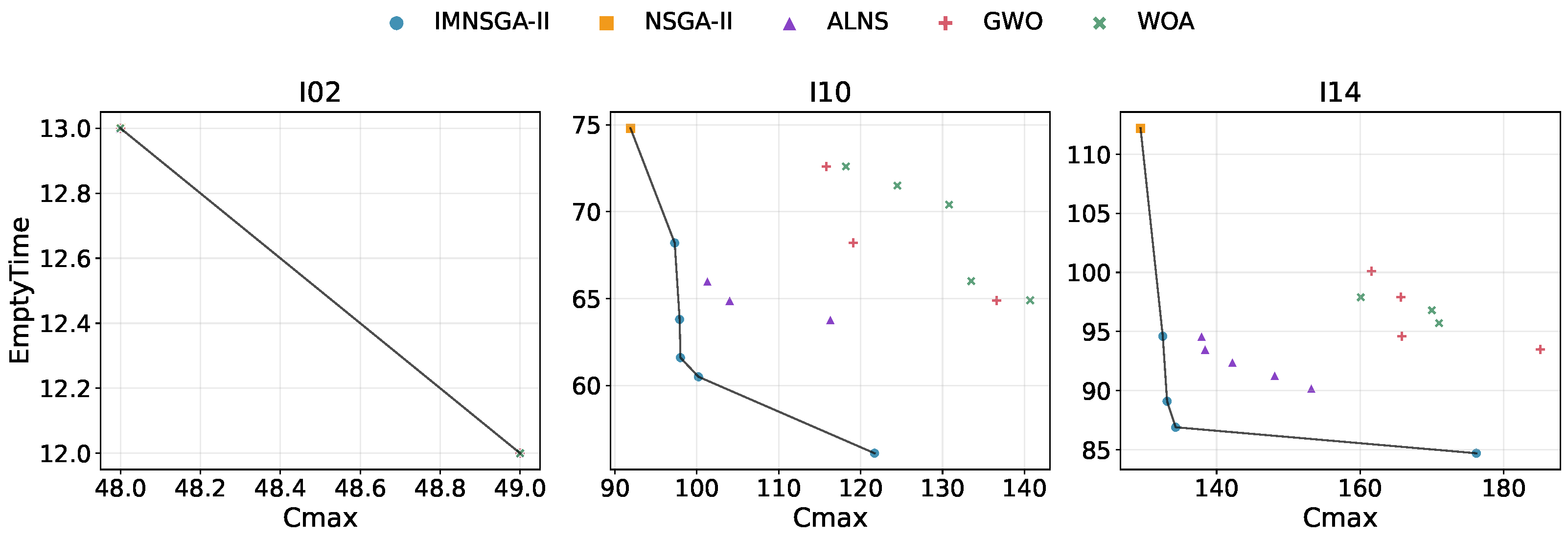
When Table 7 and Table 8 are considered together, a clear conclusion emerges. The ablation study shows that the superiority of IMNSGA-II originates from the proposed improvement modules themselves, while the comparative study further confirms that these internal enhancements can be translated into a consistent advantage over several representative metaheuristics under the same decoding framework and time budget. To visually illustrate the differences among the compared algorithms, Figure 5 shows the Pareto front distributions for small-, medium-, and large-scale instances. It can be observed that IMNSGA-II forms the outer front in most cases, corresponding to shorter completion times and lower empty travel times.

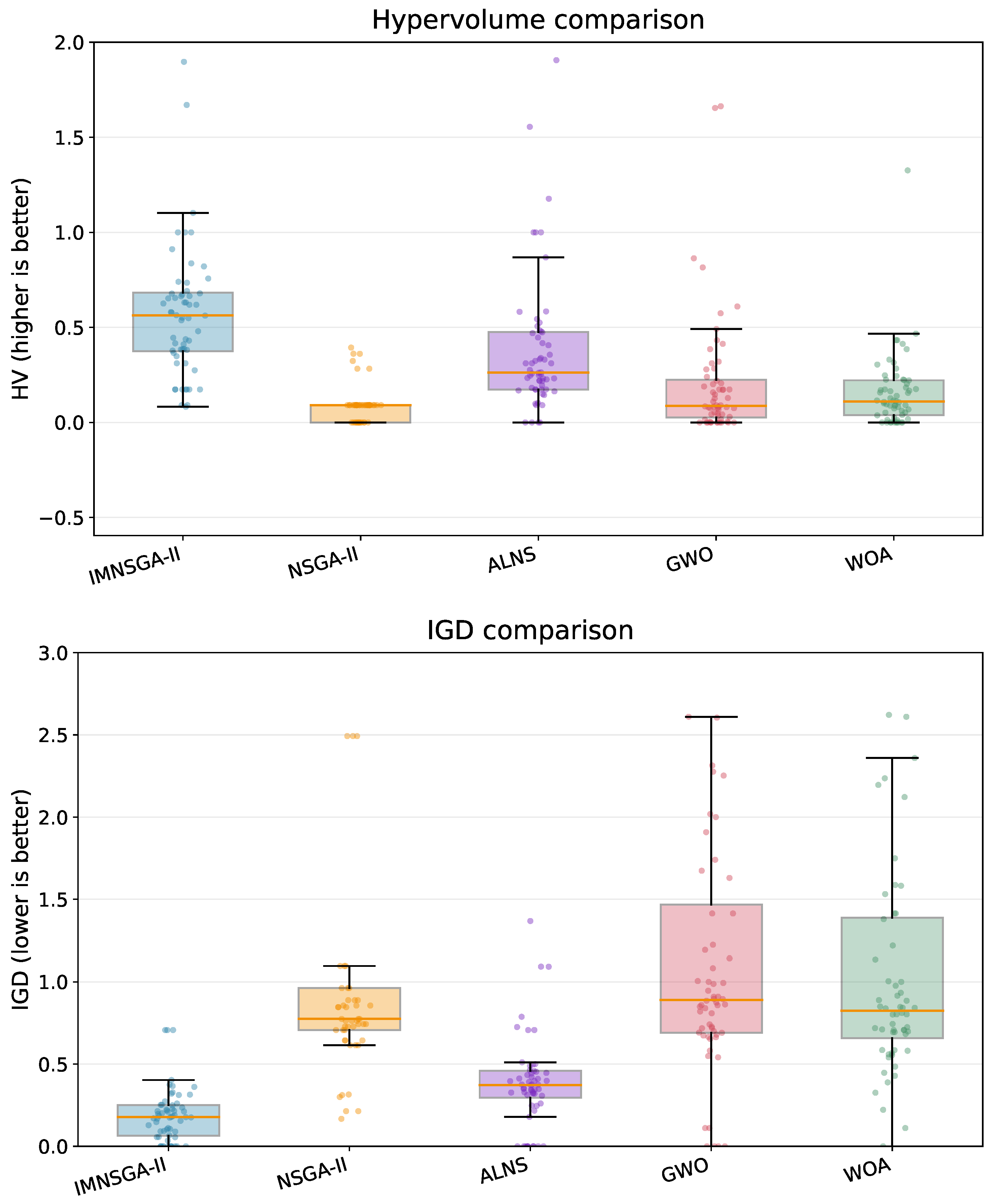
In addition, the boxplots of the performance indicators obtained over repeated runs on all benchmark instances are shown in Figure 6, where isolated points denote outliers. The upper panel shows that the HV values of IMNSGA-II are overall higher than those of the other four algorithms, whereas the lower panel shows that its IGD values are overall lower. This indicates that IMNSGA-II can approximate the reference front more closely while maintaining a more uniform distribution of solutions. Overall, the results demonstrate that IMNSGA-II achieves a better balance between convergence and diversity than the competing algorithms.

Figure 6 indicates that the performance advantage of IMNSGA-II remains stable over repeated runs.

Additionally, run-level RPI values are used for the statistical analysis of HV and IGD. For each run-level sample $s=(\mathrm{instance},\mathrm{seed})$, the RPI of algorithm i is defined as

$${\mathrm{RPI}}_{i,s}=\left\{\begin{array}{cc}{\displaystyle \frac{H{V}_s^{max}-H{V}_{i,s}}{H{V}_s^{max}}}\times 100\%,\hfill & \mathrm{for}\mathrm{HV},\hfill \\ {\displaystyle \frac{IG{D}_{i,s}-IG{D}_s^{min}}{IG{D}_s^{min}}}\times 100\%,\hfill & \mathrm{for}\mathrm{IGD},\hfill \end{array}\right.$$

(47)

where $H{V}_s^{max}$ is the maximum HV value and $IG{D}_s^{min}$ is the minimum IGD value obtained by all compared algorithms on sample s. Smaller RPI values therefore indicate better performance, and an RPI value of zero means that the algorithm is the best on that run. ANOVA on the run-level RPI values shows significant differences among the compared algorithms for both HV and IGD ($p<0.001$ for both metrics). In addition, paired t-tests at the 95% confidence level are conducted between IMNSGA-II and each baseline based on the corresponding RPI values, as reported in

Table 9. Paired t-test based on run-level RPI values in the comparative experiments.

Algorithms	HV	IGD
IMNSGA-II vs. NSGA-II	<0.001	<0.001
IMNSGA-II vs. ALNS	<0.001	0.004
IMNSGA-II vs. MOGWO	<0.001	0.003
IMNSGA-II vs. MOWOA	<0.001	0.004

. All p-values are below 0.05, indicating that IMNSGA-II statistically outperforms NSGA-II, ALNS, MOGWO, and MOWOA in terms of both HV and IGD.

7. Conclusions and Future Work

This study examines the assembly workshop scheduling problem of blocking and constrained material handling resources, with makespan and total empty travel time as optimization objectives. Unlike scheduling models that only consider production sequencing, the problem studied in this paper additionally accounts for multiple constraints, including finite buffer capacities of production resources and service area restrictions of material handling resources. To this end, an improved memetic NSGA-II algorithm is developed. By integrating the VNS-SA local search mechanism into the global evolutionary framework of NSGA-II, the proposed method achieves strong performance on this class of problems. A series of experiments is conducted to validate the effectiveness of the proposed model and method: optimal solutions are first obtained on small-scale instances using the Gurobi commercial solver. In the decoupling experiments, scheduling production and transportation separately leads to a significant deterioration in performance metrics, demonstrating the necessity of integrated scheduling. The ablation experiments show that removing the newly introduced components of the algorithm also results in varying degrees of performance degradation. Finally, in comparative experiments against other classical algorithms, the proposed algorithm achieves superior overall performance. Although the current research is based on a deterministic model, it can still adapt to minor operational fluctuations to a limited extent. Firstly, this is because the framework inherently considers various practically significant constraints and their mutual coupling relationships, making the scheduling scheme still somewhat feasible under slight time deviations. Secondly, it is because the event-driven decoding mechanism, even in the face of short delays, only needs to sequentially roll the remaining tasks without having to reconstruct the entire plan. Therefore, the current deterministic model still retains limited adaptability in a workshop environment with minor disturbances.

Future research may consider more realistic and dynamic assembly workshop environments. For instance, stochastic processing times, uncertain transportation times, machine breakdowns, and urgent order insertions could be incorporated to improve the practical relevance of the model. A broader set of optimization objectives, including energy consumption, carbon emissions, and equipment utilization balance, could also be introduced. From an algorithmic perspective, reinforcement learning could be employed to more intelligently learn how to control the local search budget and neighborhood structures, so as to handle larger-scale and more dynamic scheduling problems. In addition, future work could investigate parallel implementations of IMNSGA-II, such as GPU- or MPI-based acceleration, to further improve computational efficiency for larger-scale instances.

References

1. Gao, Q.; Hu, H.; Liu, J.; Zhuang, C.; Ding, H.; Li, H. Distributed assembly shop scheduling problem for complex products considering multiskilled worker assignment and transportation time. Int. J. Prod. Res. 2024, 1–23. [Google Scholar] [CrossRef] [Scilit]
2. Yang, H.; Fujimura, S. Multi-Objective Comprehensive Approach for Flexible Assembly Job Shop Scheduling Problem with AGVs. IEEJ Trans. Electr. Electron. Eng. 2026, 21, 235–248. [Google Scholar] [CrossRef] [Scilit]
3. Homayouni, S.M.; Fontes, D.B.M.M. Production and transport scheduling in flexible job shop manufacturing systems. J. Glob. Optim. 2021, 79, 463–502. [Google Scholar] [CrossRef] [Scilit]
4. Meng, L.; Cheng, W.; Zhang, B.; Zou, W.; Fang, W.; Duan, P. An improved genetic algorithm for solving the multi-AGV flexible job shop scheduling problem. Sensors 2023, 23, 3815. [Google Scholar] [CrossRef] [Scilit] [PubMed]
5. Fu, J.; Yang, B.; Chang, Z.; Zhang, Y.; Wang, J.; Wang, X.; Wang, L. Integrated Production–Logistics Scheduling in Flexible Assembly Shops Using an Improved Genetic Algorithm. Machines 2025, 13, 1090. [Google Scholar] [CrossRef] [Scilit]
6. Ge, S.; Zhang, H.; Xu, Z.; Yang, Z. A Multi-Objective Artificial Bee Colony Algorithm Incorporating Q-Learning Search for the Flexible Job Shop Scheduling Problems with Multi-Type Automated Guided Vehicles. Appl. Sci. 2025, 15, 10948. [Google Scholar] [CrossRef] [Scilit]
7. Ahmadi-Javid, A.; Haghi, M.; Hooshangi-Tabrizi, P. Integrated job-shop scheduling in an FMS with heterogeneous transporters: MILP formulation, constraint programming, and branch-and-bound. Int. J. Prod. Res. 2024, 62, 3288–3304. [Google Scholar] [CrossRef] [Scilit]
8. Liao, R.; Liu, J.; Qiu, J.; Peng, C. Collaborative optimisation framework for multi-stage flexible assembly shop scheduling with mixed production pattern. Int. J. Prod. Res. 2025, 63, 9070–9088. [Google Scholar] [CrossRef] [Scilit]
9. Deb, K.; Pratap, A.; Agarwal, S.; Meyarivan, T. A fast and elitist multiobjective genetic algorithm: NSGA-II. IEEE Trans. Evol. Comput. 2002, 6, 182–197. [Google Scholar] [CrossRef] [Scilit]
10. Mladenović, N.; Hansen, P. Variable neighborhood search. Comput. Oper. Res. 1997, 24, 1097–1100. [Google Scholar] [CrossRef] [Scilit]
11. Kirkpatrick, S.; Gelatt, C.D.J.; Vecchi, M.P. Optimization by Simulated Annealing. Science 1983, 220, 671–680. [Google Scholar] [CrossRef] [Scilit]
12. Deb, K.; Jain, H. An Evolutionary Many-Objective Optimization Algorithm Using Reference-Point-Based Nondominated Sorting Approach, Part I: Solving Problems with Box Constraints. IEEE Trans. Evol. Comput. 2014, 18, 577–601. [Google Scholar] [CrossRef] [Scilit]
13. Yang, B.; Chen, J.; Xiao, X.; Li, S.; Ren, T. An enhanced NSGA-II driven by deep reinforcement learning to mixed flow assembly workshop scheduling system with constraints of continuous processing and mold changing. Systems 2025, 13, 659. [Google Scholar] [CrossRef] [Scilit]
14. Han, X.; Cheng, W.; Meng, L.; Zhang, B.; Gao, K.; Zhang, C.; Duan, P. A dual population collaborative genetic algorithm for solving flexible job shop scheduling problem with AGV. Swarm Evol. Comput. 2024, 86, 101538. [Google Scholar] [CrossRef] [Scilit]
15. Pan, Z.; Wang, L.; Zheng, J.; Chen, J.F.; Wang, X. A learning-based multipopulation evolutionary optimization for flexible job shop scheduling problem with finite transportation resources. IEEE Trans. Evol. Comput. 2022, 27, 1590–1603. [Google Scholar] [CrossRef] [Scilit]
16. Wang, H.; Peng, T.; Li, X.; He, J.; Liu, W.; Tang, R. An integrated simulation–optimization method for flexible assembly job shop scheduling with lot streaming and finite transport resources. Comput. Ind. Eng. 2025, 200, 110790. [Google Scholar]
17. Ham, A. Transfer-robot task scheduling in job shop. Int. J. Prod. Res. 2021, 59, 813–823. [Google Scholar] [CrossRef] [Scilit]
18. Fatemi-Anaraki, S.; Tavakkoli-Moghaddam, R.; Foumani, M.; Vahedi-Nouri, B. Scheduling of multi-robot job shop systems in dynamic environments: Mixed-integer linear programming and constraint programming approaches. Omega 2023, 115, 102770. [Google Scholar] [CrossRef] [Scilit]
19. Zeng, C.; Tang, J. Blocking job shop cell scheduling with automated guided vehicles. In Proceedings of the 11th World Congress on Intelligent Control and Automation; IEEE: Piscataway, NJ, USA, 2014; pp. 438–442. [Google Scholar]
20. Valencia, J.; Rodríguez-Velásquez, E. The Estimation Distribution Algorithm for the Blocking Job Shop Scheduling Problem. Appl. Sci. 2025, 15, 9339. [Google Scholar] [CrossRef] [Scilit]
21. Yang, S.; Meng, L.; Ullah, S.; Zhang, C.; Sang, H.; Zhang, B. MILP modeling and optimization of three-stage flexible job shop scheduling problem with assembly and AGV transportation. Chin. J. Mech. Eng. 2025, 38, 115. [Google Scholar] [CrossRef] [Scilit]
22. Fontes, D.B.M.; Homayouni, S.M. Joint production and transportation scheduling in flexible manufacturing systems. J. Glob. Optim. 2019, 74, 879–908. [Google Scholar]
23. Wessén, J.; Carlsson, M.; Schulte, C.; Flener, P.; Pecora, F.; Matskin, M. A constraint programming model for the scheduling and workspace layout design of a dual-arm multi-tool assembly robot. Constraints 2023, 28, 71–104. [Google Scholar]
24. Dauzère-Pérès, S.; Ding, J.; Shen, L.; Tamssaouet, K. The flexible job shop scheduling problem: A review. Eur. J. Oper. Res. 2024, 314, 409–432. [Google Scholar] [CrossRef] [Scilit]
25. Zhang, S.; Wang, S. Flexible assembly job-shop scheduling with sequence-dependent setup times and part sharing in a dynamic environment: Constraint programming model, mixed-integer programming model, and dispatching rules. IEEE Trans. Eng. Manag. 2018, 65, 487–504. [Google Scholar]
26. Lin, W.; Deng, Q.; Han, W.; Gong, G.; Li, K. An effective algorithm for flexible assembly job-shop scheduling with tight job constraints. Int. Trans. Oper. Res. 2022, 29, 496–525. [Google Scholar] [CrossRef] [Scilit]
27. Fattahi, P.; Bagheri Rad, N.; Daneshamooz, F.; Ahmadi, S. A new hybrid particle swarm optimization and parallel variable neighborhood search algorithm for flexible job shop scheduling with assembly process. Assem. Autom. 2020, 40, 419–432. [Google Scholar] [CrossRef] [Scilit]
28. Shi, F.; Zhao, S.; Meng, Y. Hybrid algorithm based on improved extended shifting bottleneck procedure and GA for assembly job shop scheduling problem. Int. J. Prod. Res. 2020, 58, 2604–2625. [Google Scholar]
29. Yuan, M.; Zheng, L.; Huang, H.; Zhou, K.; Pei, F.; Gu, W. Research on flexible job shop scheduling problem with AGV using double DQN. J. Intell. Manuf. 2025, 36, 509–535. [Google Scholar]
30. Dong, X.; Wan, G.; Zeng, P. A heuristic-assisted deep reinforcement learning algorithm for flexible job shop scheduling with transport constraints. Complex Intell. Syst. 2025, 11, 210. [Google Scholar] [CrossRef] [Scilit]
31. Akopov, A.S. MBHGA: A matrix-based hybrid genetic algorithm for solving an agent-based model of controlled trade interactions. IEEE Access 2025, 13, 26843–26863. [Google Scholar] [CrossRef] [Scilit]
32. Aguilar-Rivera, A. A GPU fully vectorized approach to accelerate performance of NSGA-2 based on stochastic non-domination sorting and grid-crowding. Appl. Soft Comput. 2020, 88, 106047. [Google Scholar] [CrossRef] [Scilit]
33. Meng, L.; Zhang, C.; Zhang, B.; Gao, K.; Ren, Y.; Sang, H. MILP modeling and optimization of multi-objective flexible job shop scheduling problem with controllable processing times. Swarm Evol. Comput. 2023, 82, 101374. [Google Scholar] [CrossRef] [Scilit]
34. Ciro, G.C.; Dugardin, F.; Yalaoui, F.; Kelly, R. A NSGA-II and NSGA-III comparison for solving an open shop scheduling problem with resource constraints. IFAC-PapersOnLine 2016, 49, 1272–1277. [Google Scholar]
35. Almeida, F.S.d.; Nagano, M.S. An ALNS to optimize makespan subject to total completion time for no-wait flow shops with sequence-dependent setup times. Top 2024, 32, 304–322. [Google Scholar]
36. Komaki, G.; Kayvanfar, V. Grey Wolf Optimizer algorithm for the two-stage assembly flow shop scheduling problem with release time. J. Comput. Sci. 2015, 8, 109–120. [Google Scholar] [CrossRef] [Scilit]
37. Jiang, T.; Zhang, C.; Sun, Q.M. Green job shop scheduling problem with discrete whale optimization algorithm. IEEE Access 2019, 7, 43153–43166. [Google Scholar] [CrossRef] [Scilit]
Figure 3. Main effects plot of the IGD metric and the corresponding S/N ratio obtained from the Taguchi L9( 3 4 ) parameter calibration study. Here, Level 1, Level 2, and Level 3 denote the first, second, and third settings of each factor, respectively.
Applsci 16 05343 g003
Figure 4. Comparison of Pareto fronts in the decoupling experiments.
Applsci 16 05343 g004
Figure 5. Comparison of Pareto fronts for small-, medium-, and large-scale instances in the comparative experiments.
Applsci 16 05343 g005
Figure 6. Run-level boxplots of HV and IGD in the comparative experiments.
Applsci 16 05343 g006