Article

Non-Intrusive Electrical Monitoring for the Real-Time Estimation of Production Parameters in a Sheet Metal Stamping Line

by
Camilo Carrillo González
1,*,
Eloy Díaz Dorado
1,
Adrián Juan Pérez Peña
1,
José Cidrás Pidre
1,
Cristina Isabel Martínez Castañeda
2 and
José Florencio Sánchez Rúa
2
1
Research Group on Efficient and Digital Engineering, University of Vigo, 36310 Vigo, Spain
2
Stellantis Group, 36210 Vigo, Spain
*
Author to whom correspondence should be addressed.
Appl. Sci. 2026, 16(11), 5336; https://doi.org/10.3390/app16115336
Submission received: 11 March 2026 / Revised: 12 May 2026 / Accepted: 22 May 2026 / Published: 26 May 2026
(This article belongs to the Section Electrical, Electronics and Communications Engineering)

Featured Application

This paper presents a non-intrusive, real-time method for identifying the part being produced in a metal stamping line and for estimating both cycle time and per-cycle energy consumption. The approach integrates machine-learning techniques, specifically Support Vector Machine (SVM) classification supported by features from the time domain and the Continuous Wavelet Transform (CWT).

Abstract

Metal forming processes, characterized by high energy consumption, are widely used in modern manufacturing. In this context, methods for monitoring the operational state and cycle-dependent metrics of manufactured parts are essential for implementing energy optimization strategies. Such strategies require moving away from time-aggregated energy assessments, which fail to capture part-level variability, toward analyses at the granularity of individual parts. This article introduces a non-intrusive methodology to enable the identification, in real time, of the part under production and to estimate cycle time and energy consumption per part. The method relies on electrical measurements taken at the switchboards. The RMS current and power values are the inputs to a machine-learning (ML) approach that identifies the part in production. To this end, the time-domain and time–frequency-domain features extracted from the signals are employed to train a Support Vector Machine (SVM) classifier that achieves a test accuracy of 99.9%. Next, the approach estimates cycle time and energy per cycle in real time. Approximately 58,000 production cycles, corresponding to several part types, were characterized. The proposed approach demonstrates that part-level identification and per-cycle energy estimation can be achieved in real time using only electrical measurements in an industrial process.

1. Introduction

Metal forming is a fundamental process in manufacturing, particularly in sectors such as vehicle production and aviation [1]. Such operations are characterized by high energy consumption due to the low efficiency of the metal forming presses [2]. In this context, monitoring consumption is essential in order to optimize efficiency, especially if, as this article proposes, the part in production is detected along with its cycle time and the energy per cycle.
Energy analysis in industrial applications is a typical domain for artificial intelligence (AI) techniques [3]. With respect to energy consumption estimation, AI-based applications are typically focused on long-term consumption forecasting, whereas real-time monitoring is more often oriented toward other aspects, such as product quality assessment [4,5]. For instance, in [6], convolutional neural networks (CNNs) are applied to electrical signals to identify the operational state of the painting sector in an automotive manufacturing plant at daily and weekly timescales. On the other hand, ref. [7] presents an example of a manufacturing process in which CNNs are used to classify process conditions by extracting parameters from acoustic signals in real time; however, this approach is not directly related to energy consumption estimation.
Previous works of the research group, see [8,9], have shown that detailed analysis of metal forming presses from electrical measurements and the use of Neural Network (NN) techniques have enabled identification of both the operating state of the presses and a breakdown of the energy consumed per cycle to give a precise characterization of the machine’s dynamic behavior. However, this analysis is performed offline, using records acquired with a commercial power quality analyzer, which allows the extraction of statistical results but does not enable real-time implementation. In contrast, the present article proposes the use of Support Vector Machine (SVM) techniques, which, in addition to their widespread adoption in industrial applications, offer several advantages over NNs, such as lower data requirements and greater robustness to noise [4,5,10].
Accordingly, this paper presents a method for the real-time identification of the parts being produced, their production rate, and the energy consumption per manufactured part. For the classification task related to identifying the part under production, Support Vector Machine (SVM) techniques are employed, which are widely used in the manufacturing industry [10,11], and are combined here with time-domain features and a time–frequency analysis based on the Continuous Wavelet Transform (CWT). Finally, the production time required to manufacture each part and its associated energy consumption are obtained.
Additionally, the proposed system addresses a limitation associated with the slow update rate of conventional electrical measurements such as root mean square (RMS). Power quality analyzers commonly comply with the IEC 61000-4-30 standard [12], which establishes minimum intervals of ten cycles (for a 50 Hz power system) when calculating magnitudes such as RMS voltage or RMS current. Although this requirement is adequate for electrical supply supervision, it does not record in sufficient detail the rapid current variations that occur throughout the different phases of the metal forming cycle. These short-lived phenomena, associated with abrupt load changes (such as the mechanical impact during part forming), contain relevant information not only on the machine’s operational state but also on its instantaneous energy behavior. Therefore, limited acquisition at ten-cycle intervals can lead to an underestimation of the effective energy consumed and a loss of useful information for accurately identifying working regimes.
With the aim of addressing the limitations of conventional measurement systems and advancing the energy characterization of metal forming presses, this study presents the development of a high-speed electrical parameter measurement system capable of real-time processing, designed specifically to acquire one-cycle RMS voltage and current signals. The system enables automatic classification of the production state using ML techniques and provides real-time estimates of both the cycle time and the associated energy consumption.
The article is organized as follows: Section 2 describes the electrical parameter measurement system developed; Section 3 details the preparation of the datasets and the classification procedure; Section 4 presents the estimation methods for the cycle time and its associated energy; Section 5 shows the results obtained; and, finally, Section 6 contains the conclusions.

2. Electrical Parameter Measurement System

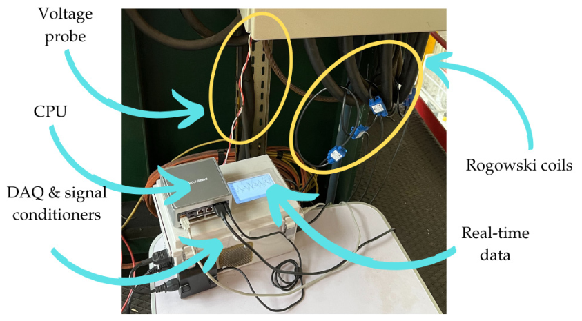
The sheet metal stamping line analyzed in this article is fed from a main switchboard that has four dependent electrical panels that supply various subprocesses or stamping stages. To obtain the line’s total consumption, current probes (Rogowski type) and a voltage probe were installed in the main switchboard (see Figure 1). Furthermore, to facilitate detection of the part in production, a current probe was installed in the switchboard of the first process stage. The voltage and current signals were sent to a data-acquisition system (DAQ) and a processing unit (CPU), which was responsible for real-time energy calculations, cycle-time estimation and part detection. The measurement system also had a display interface that allowed the results to be monitored. The main features of the equipment developed are shown in Table 1, which highlights the high speed of the power and RMS value calculations as well as its capacity to implement algorithms for detecting parts in production, with their corresponding cycle time and energy.
This equipment enabled the development of non-intrusive detection systems for the production characteristics of a specific process, such as the stamping line addressed in this article, which allowed implementation without interrupting the operation of the installation.

3. Dataset Preparation and Classification

3.1. Characterization and Time Segmentation

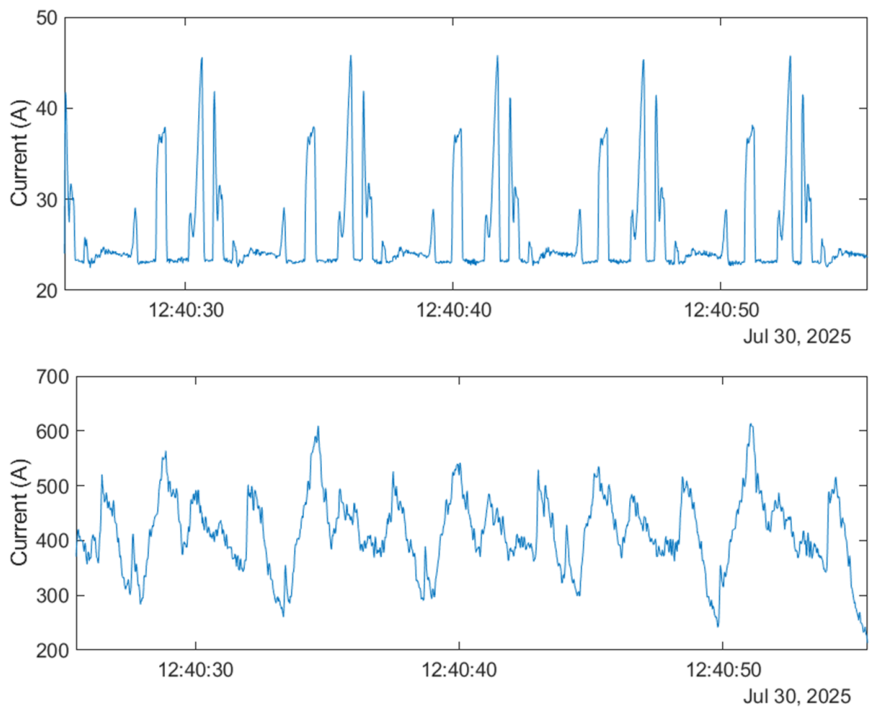
Initial analysis of the current signals acquired showed a behavior that, although cyclical in both cases, was markedly non-stationary on the main switchboard (attributable to the aggregate nature of the consumption by multiple pieces of equipment) and more stable on the first process-stage switchboard. Figure 2 shows an example of the current signals acquired simultaneously on both switchboards during several production cycles while forming a part.
In order to structure the signals for processing compatible with real-time implementation, they were segmented into 20 s windows. This duration was chosen after verifying that the typical production cycle time ranged between five and seven seconds per part, which ensured that each window contained at least two complete cycles.

3.2. Dataset Labeling and Construction

To permit dataset construction, the company provided the part reference being produced at each time instant, which made it possible to associate a label with each 20 s window corresponding to the manufactured part. Although nine distinct parts or references were analyzed (P1 to P9), a total of ten classes were used: the nine identified parts and an additional class called “idle” (IDLE), which was assigned to those windows in which no part was being processed. The inclusion of this class prevented the classifier from incorrectly assigning unproductive periods to a specific part and enabled detection of inactive states, a necessary requirement for the subsequent calculation of cycle-dependent metrics, such as the cycle time.
Despite data being compiled for model construction over three months, actual production was not evenly distributed to reflect the different classes, and therefore some parts appear more often than others. To avoid bias while training the classifiers, the dataset was balanced by randomly downsampling the majority classes until an equal number of samples per class was reached. Although downsampling may lead to information loss in majority classes, it remains a widely adopted strategy for mitigating class imbalance problems [13].
A total of seven thousand 20 s windows were used for feature extraction, with 700 representations of each class, using information from both the main switchboard and the first process-stage switchboard.

3.3. Feature Extraction in the Time and Time–Frequency Domains

To address the variability of the current signals within each window, classical spectral analysis methods such as the Fourier Transform are insufficient as they assume stationarity and do not adequately capture time-varying frequency components [14].
A common alternative for analyzing non-stationary signals is the Short-Time Fourier Transform, based on the application of a sliding window on the signal. Although this technique provides information in both the time and the frequency domains, it has a fundamental limitation: the window size is fixed, which imposes a constant time or frequency resolution throughout the signal. This approach is not suitable for highly dynamic processes, where the aim is to capture with precision both time information in high-frequency transients and more-persistent patterns in low-frequency bands [15].
To overcome this trade-off between time and frequency resolution, the Continuous Wavelet Transform (CWT) was employed, as it has been shown to outperform other techniques in the analysis of non-stationary signals [7,16]. The CWT calculates the similarity between the signal and a base function (mother wavelet) shifted and scaled in time (wavelet), which enables adaptive decomposition: the small scales correspond to high-frequency components, while the large scales represent low-frequency variations [17]. These scales are logarithmically distributed, and the choice of their density introduces a trade-off between frequency resolution and computational cost.
In this study, the Morlet wavelet was chosen as the mother wavelet as it represents the best balance between time and frequency resolution [18]. Analysis was performed using the MATLAB Wavelet Toolbox (R2025a) [19], setting a value of four voices per octave to control the scale density. Given this configuration and the RMS computation rate (50 Hz, i.e., one value per cycle), the software automatically determined the range of frequencies considered, which in this case spanned from approximately 0.14 to 18.41 Hz, leading to a total of 29 scales (seven octaves in addition to the minimum scale). Statistical features were extracted from the coefficients obtained in each scale: mean, skewness, kurtosis, RMS and variance. Previous studies [20,21] have demonstrated the effectiveness of such statistical features derived from wavelet coefficients when representing non-stationary dynamics.
Furthermore, to enhance signal representation, some of the most commonly used descriptors from the time domain were included in the classification: mean, range, RMS, variance, skewness and kurtosis.

3.4. Normalization and Partitioning

After feature extraction, each dataset was divided into two subsets: 85% of the samples were used for training and validation, while the remaining 15% were reserved for final testing.
Since the extracted features exhibited heterogeneous numerical ranges, Z-score normalization was applied [22]. The normalization parameters (mean and standard deviation) were computed using only the training data and subsequently applied to the test set, ensuring that no information leakage occurred.
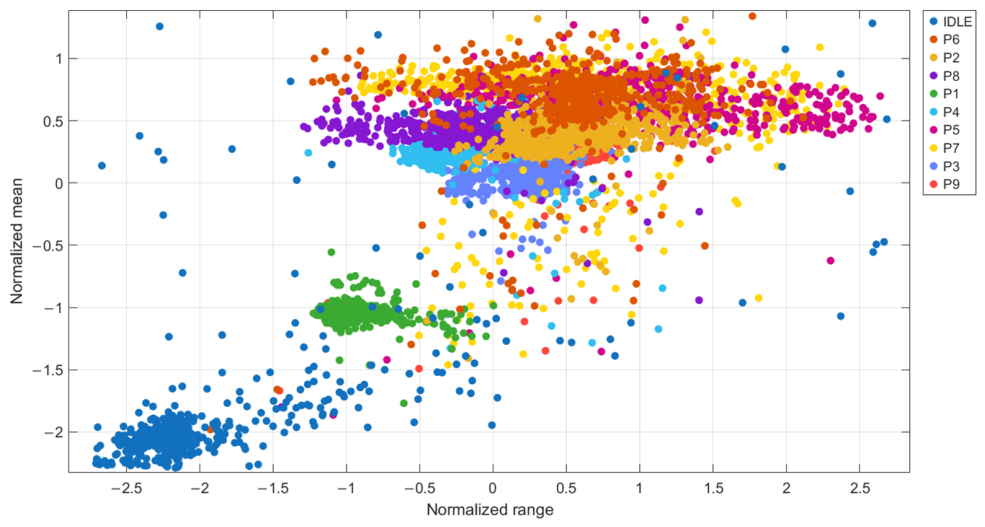
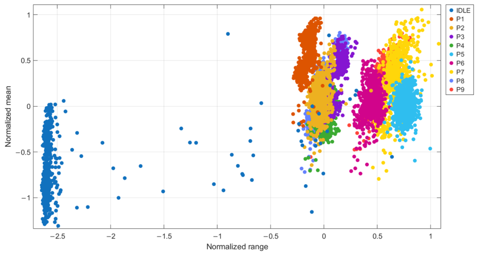
Figure 3 and Figure 4 show the scatter plots of the training samples for both datasets, indicating the part in production (P1 to P9) and the idle state (IDLE). The figures show better separation in the classes corresponding to the current probe installed at the first process-stage switchboard compared to those obtained from the current probe installed at the main switchboard.

3.5. Classification Using SVM

Support Vector Machines (SVMs) are supervised learning models that have demonstrated strong performance in both regression and classification problems [23]. This model is based on the creation of a hyperplane that maximizes the margin between classes [24].
To fit the model to both datasets, the hyperparameters, which control the learning process and cannot be learned from the data, were tuned [25]. To this end, a grid search was used in combination with cross validation [21,26]. Grid search is an exhaustive search technique that evaluates different combinations of hyperparameters within a predefined space [27,28]. In this study, the error in classification was calculated for each hyperparameter combination by means of five-fold cross validation, finally selecting the set that minimized this error.
The search space included the kernel function (linear, polynomial and radial basis function (RBF)); the cost parameter (C), explored on a logarithmic scale from 0.001 to 1000, and the gamma parameter ( γ ) which was explored over the same range (only considered in the case in which the kernel function was RBF).
All the models were trained using features previously normalized by means of Z-score, following the procedure described in Section 3.4. The multiclass classification was implemented using the one-vs-one decomposition, a strategy recommended because of its good performance in multiclass problems [29].
The structure and specifications of both models are summarized in Table 2.

4. Cycle Time and Energy Estimation per Part

4.1. Cycle Time Estimation

Once the model predicted that a part was being stamped, the RMS current measured at the first process-stage switchboard was used to estimate the cycle time, as this signal presented a more stable and periodic structure than the aggregated measurements from the main switchboard. Furthermore, due to the temporal averaging involved in the RMS calculation, high-frequency noise components are significantly reduced, resulting in a smoothing effect comparable to low-pass filtering. This facilitates the identification of the stamping cycles.
A peak-detection algorithm was applied to the signal, based on the identification of local maxima and their filtering according to amplitude and temporal constraints [30]. Specifically, two criteria were used: a minimum peak distance and the selection of representative peak height.
The minimum peak distance was set to 4.4 s. This value was determined from the analysis of the stamping process, under the assumption that two consecutive parts cannot be processed in a shorter time interval.
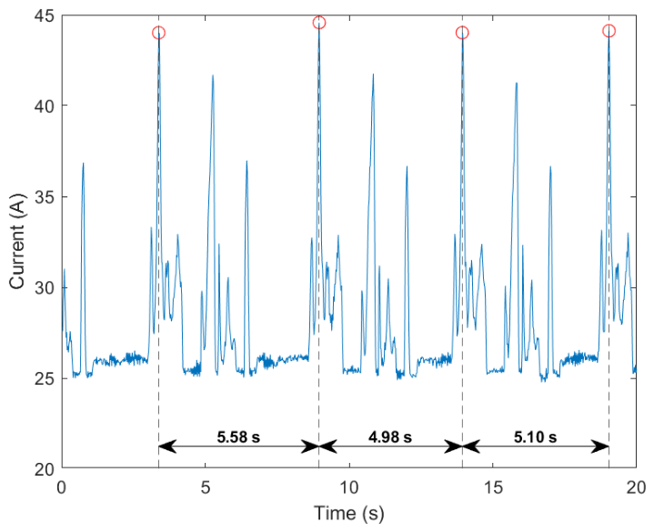
The representative peaks are selected, in most cases, using peak values that fall within a given percentage (e.g., 95%) of the maximum value recorded in each window. Under these conditions, each detected peak is considered representative of a production cycle, and the cycle time is defined as the time interval between consecutive peaks. Figure 5 illustrates an example of the proposed procedure. In some cases, during a part’s production, current demand exhibits two peaks that meet the defined criterion. In such cases, the peak values are sorted by amplitude, and the peak following the identified pair is selected as representative.

4.2. Energy Estimation per Produced Part

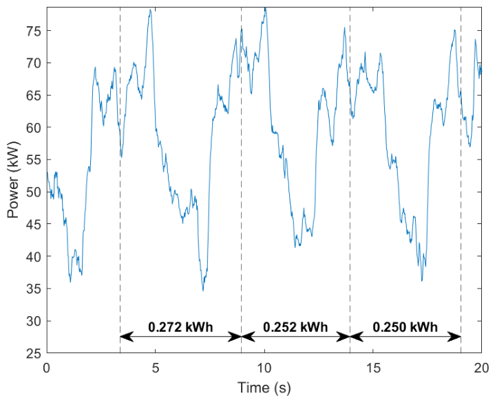
To estimate the energy associated with each cycle, the timestamps of the detected peaks were synchronized with the aggregated active power measured on one phase of the main switchboard, as both signals were acquired simultaneously and shared the same timestamp. Therefore, the total energy absorbed in each cycle was calculated from the active power measured between two consecutive peaks (see Appendix A). An example of this synchronization between both signals can be seen in Figure 6.

5. Results

5.1. Estimation of the Line State

Hyperparameter optimization by grid search produced, for both datasets, SVM models with linear kernels. The final values selected for each model are given in Table 3.
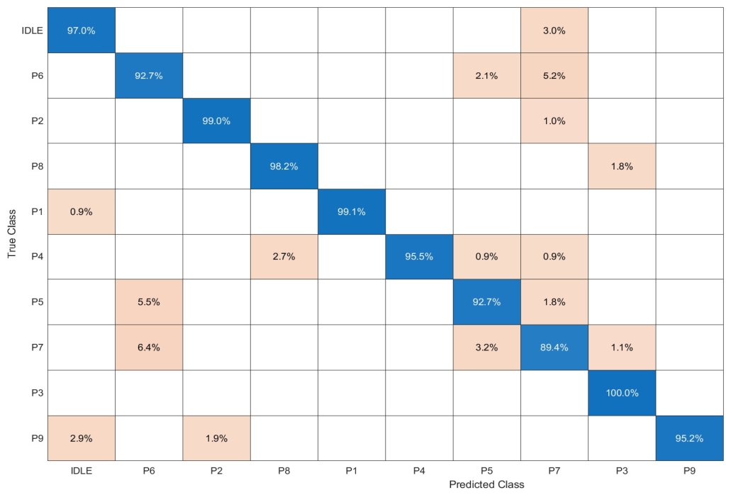
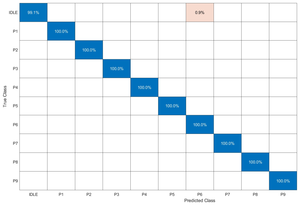
Model performance was evaluated on the reserved test set. The classifier trained on aggregated measurements from the main switchboard achieved a test accuracy of 96%. Its confusion matrix (Figure 7) shows limited separability among certain classes, particularly parts P5, P6, and P7. In contrast, the model trained on disaggregated measurements from the first process-stage switchboard reached a test accuracy of 99.9%, with only a single misclassified sample. Its confusion matrix is shown in Figure 8. To provide a more comprehensive evaluation, Table 4 reports class-wise precision, recall, and F1-score for both models.
Altogether, the results confirm that disaggregated electrical measurements, based on adding a current sensor at the first process-stage switchboard, offer greater discriminative capability for line-state classification. Therefore, this signal was selected for subsequent real-time part identification and cycle-level analysis.

5.2. Estimation of Cycle Time and Energy per Cycle

From the classification undertaken on the data acquired over 432 h of operation, excluding non-productive periods, approximately 58,000 production cycles were identified. Both the cycle time and the demanded energy were estimated for each cycle, following the procedures described in Section 4.1 and Section 4.2.
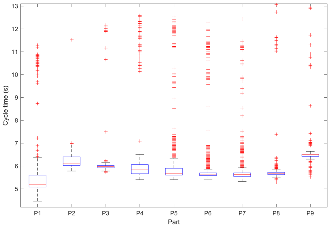
Figure 9 gives the cycle-time boxplots by part type, revealing differences in both the median cycle time and its dispersion.
To complement the graphic analysis, Table 5 summarizes the main descriptive statistics for the cycle time by part type, while Table 6 contains the values corresponding to the electrical energy consumed per cycle. In both cases, the mean is shown along with the 5th and 95th percentiles, which makes it possible to characterize the behavior and variability of each part.
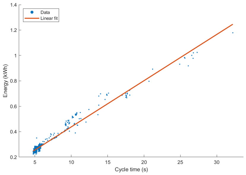
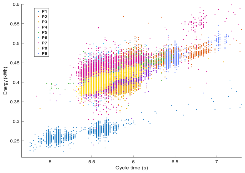
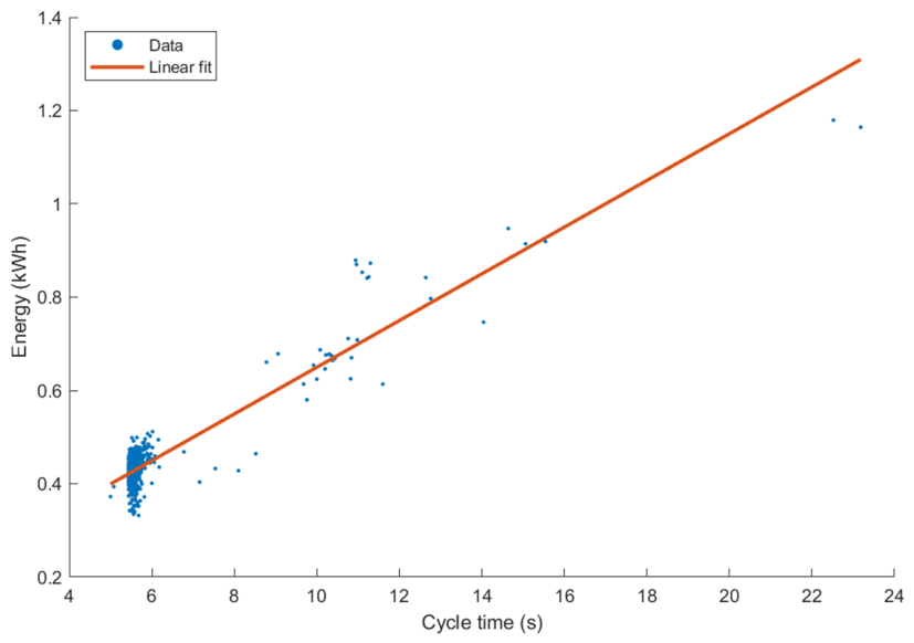
Figure 10 shows the energy consumed against cycle time, where a positive relationship between both magnitudes can be observed. This relationship can be adequately approximated by a linear model. To quantify this behavior, the coefficient of determination R2 was evaluated for each part type; the resulting values ranged between 0.79 and 0.96, confirming a strong linear relationship between both variables.
Figure 11 and Figure 12 depict two representative examples corresponding to the cases with the smallest and largest values of R2, respectively. These results can be used to adjust cycle time in terms of energy efficiency.

5.3. Real-Time Operation

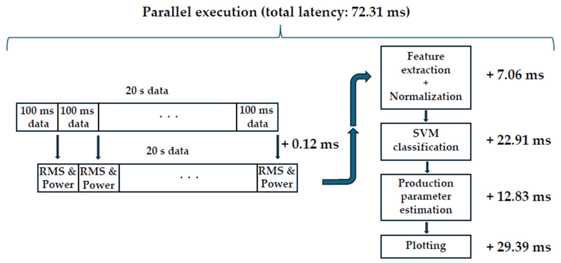
To evaluate the real-time capability of the proposed system, the computational latency of the complete processing pipeline was measured. The execution time was decomposed into five stages: RMS and power computation (executed in parallel with the remaining tasks), feature extraction and normalization, SVM inference, production-parameter estimation and plotting. The measurements showed a total processing latency of 72.31 ms from the moment the DAQ completed the acquisition of the latest data block until the results were displayed. Figure 13 summarizes the execution times associated with each processing stage.
For reference, related approaches based on feature extraction and classification have reported processing times on the order of several hundred milliseconds [7], whereas the proposed implementation achieved substantially lower latency under the evaluated conditions.
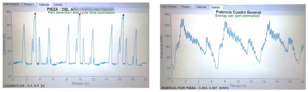
Figure 14 shows screenshots extracted from [31] corresponding to the electrical parameter measurement system display interface during real-time operation. The interface provides an integrated real-time visualization of electrical signals acquired from both switchboards, the classification result (the part in production), the detected production cycles, and their duration (cycle time) and associated energy.

6. Conclusions

This study develops and implements a high-speed measurement system for electrical parameters, capable of acquiring power and RMS values every 20 ms, in addition to allowing the implementation of algorithms to characterize parts in production in real time.
The detection algorithm for parts in production relies exclusively on the current signals acquired by the monitoring system. Features from both the time–frequency domain (via CWT) and the time domain are extracted to train SVM classifiers, whose hyperparameters were selected by grid search to identify the state of the line. The resulting models show notable performance, particularly in the disaggregated dataset (corresponding to the first process stage), where a test accuracy of 99.9% was reached. Nevertheless, the dataset was balanced through downsampling of majority classes, which may reduce the variability present in real production conditions. Therefore, additional validation under imbalanced production scenarios is required to further assess the generalization capability of the model.
Once the state of the line was identified, a peak-detection algorithm was applied to estimate the cycle time. As the electrical measurements from both switchboards are synchronized, it is possible to associate each cycle with its individual energy consumption.
This procedure enables real-time disaggregation at the part level, obtaining both its cycle time and the energy consumed. In this way, through non-intrusive techniques and the use of ML algorithms (SVM with linear kernel), a quantitative basis was provided that enabled verification of the production line’s operation and optimization of the energy demand.
Future work will focus on validating the proposed methodology over longer operating periods and under varying production conditions, as well as on optimizing the approach parameters. For instance, reducing the analysis window size may improve synchronization between part detection and the actual operation of the stamping line.


Author Contributions

Conceptualization, C.C.G. and E.D.D.; Methodology, C.C.G., E.D.D., A.J.P.P. and J.C.P.; Software, A.J.P.P.; Validation, C.C.G., E.D.D. and A.J.P.P.; Formal analysis, C.C.G., E.D.D. and A.J.P.P.; Investigation, C.C.G., E.D.D. and A.J.P.P.; Data curation, A.J.P.P.; Resources, C.I.M.C. and J.F.S.R.; Visualization, A.J.P.P.; Writing—original draft preparation, A.J.P.P.; Writing—review and editing, C.C.G., E.D.D., J.C.P., C.I.M.C. and J.F.S.R.; Supervision, C.C.G. and E.D.D.; Project administration, C.C.G.; Funding acquisition, C.C.G. All authors have read and agreed to the published version of the manuscript.

Funding

The activities described in this article were carried out within the framework of the project “FACENDO Plus (Factory Competitiveness and Electromobility Through Innovation and Digital Transformation Plus)” (IN854A 2023/01), funded by the Agencia Galega de Innovación (GAIN) of the Xunta de Galicia and co-financed by the European Union through the European Regional Development Fund (ERDF) under the ERDF Galicia 2021–2027 Operational Programme.

Institutional Review Board Statement

Not applicable.

Informed Consent Statement

Not applicable.

Data Availability Statement

The data presented in this study are not publicly available due to confidentiality agreements with the industrial partner where the measurements were conducted.

Conflicts of Interest

Cristina Isabel Martínez Castañeda and José Florencio Sánchez Rúa were employed by the company Stellantis Group. The remaining authors declare that the research was conducted in the absence of any commercial or financial relationships that could be construed as a potential conflict of interest.

Appendix A. Electrical Measurements

The main sensors for the measurement device developed for the presented approach are shown in Table A1. The uncertainty of the power measurement was estimated at 2.60%, by combining uncertainty contributions from instrument specifications under the assumption of rectangular distributions, in accordance with ISO/IEC 98-3:2008 [32].
Table A1. Main sensors of the measurement system.
ManufacturerWAGOLEMRS PRO
TypeRogowskiIntegratorDifferential
Range4 kA1000 A700 V 1
Sensitivity22.5 mV/kA -
Accuracy±0.5% and ±0.75% 20.5%±2%
Phase displacementN/A0.5°≈0° 3
1: Position x200, bandwidth 25 MHz; 2: precision class 0.5 plus a positioning error; 3: very low for 50 Hz signals.
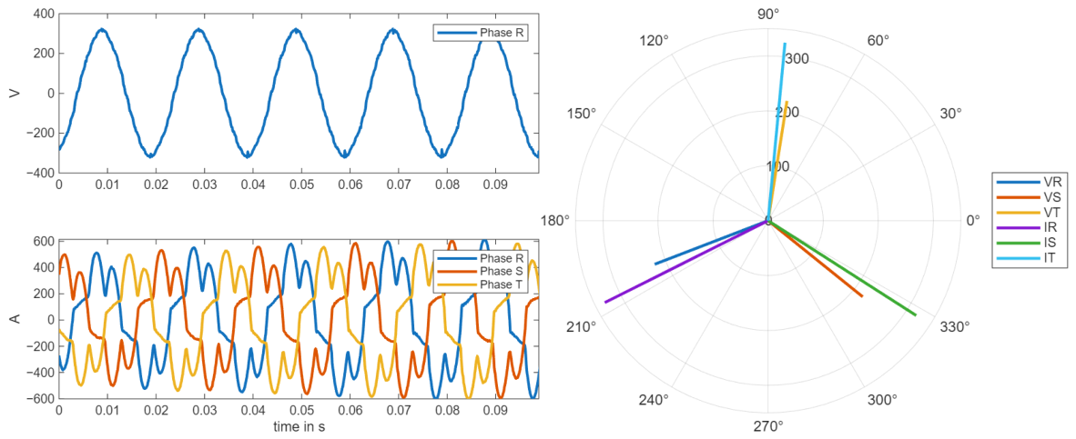
Figure A1 shows an example of the voltage and current waveforms recorded during part production. The observed waveforms are typical of three-phase converters equipped with an AC/DC input stage. The main electrical parameters of these waveforms are reported in Table A2, where RMS values, total harmonic distortion (THD), and apparent power (S) are shown, together with the values obtained from phasor analysis, namely, cos φ and the fundamental component of active power (Fund. P).
Figure A1. Waveforms of voltage and currents (left) and their corresponding phasors (right).
Applsci 16 05336 g0a1
Table A2. Main electrical parameters of recorded waveforms.
RMSTHDcos φFund. PS
Voltage221.3 V2.8%
Current R305.1 A30.6%0.9964.0 kW67.5 kVA
Current S291.3 A33.2%0.9960.6 kW64.5 kVA
Current T296.8 A30.9%1.0062.6 kW65.7 kVA
Total------187.2 kW197.7 kVA
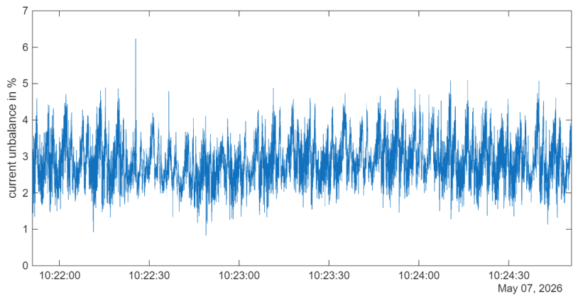
The current unbalance can be obtained from the fundamental components using IEC standards as the ratio between the negative-sequence and positive-sequence components [12]. The results for the waveforms shown in Figure A1 are presented in Table A3. As shown in Figure A2, the current unbalance remains below 5% throughout the long measurement periods. Under this condition, the average instantaneous power in a single phase can be used to estimate the total three-phase power, with only a single voltage measurement required. The systematic bias introduced by this approximation was quantified as the mean relative difference between the RMS current of phase 1 and the mean RMS current of the three phases, evaluated over N = 30,000 samples. The resulting bias was 3.81% (σ = 0.64%), which is reported separately from the instrumental measurement uncertainty and reflects the asymmetry of the installation rather than a measurement error.
Table A3. Symmetrical components and unbalance.
Zero sequence1.2 A
Positive sequence283.8 A
Negative sequence9.8 A
Unbalance3.4%
Figure A2. Current unbalance.
Applsci 16 05336 g0a2

References

  1. Zhong, J.; Zhao, K.; Liu, Z.; Li, X. Review of the research on low carbon manufacture of metal-forming equipment and future development. J. Hefei Univ. Technol. Nat. Sci. 2012, 35, 1594–1600. [Google Scholar]
  2. Gao, M.; He, K.; Li, L.; Wang, Q.; Liu, C. A Review on Energy Consumption, Energy Efficiency and Energy Saving of Metal Forming Processes from Different Hierarchies. Processes 2019, 7, 357. [Google Scholar] [CrossRef]
  3. Bunian, S.; Al-Ebrahim, M.A.; Nour, A.A. Role and Applications of Artificial Intelligence and Machine Learning in Manufacturing Engineering: A Review. Eng. Sci. 2024, 29, 1088. [Google Scholar] [CrossRef]
  4. Plathottam, S.J.; Rzonca, A.; Lakhnori, R.; Iloeje, C.O. A review of artificial intelligence applications in manufacturing operations. J. Adv. Manuf. Process. 2023, 5, e10159. [Google Scholar] [CrossRef]
  5. Bertolini, M.; Mezzogori, D.; Neroni, M.; Zammori, F. Machine Learning for industrial applications: A comprehensive literature review. Expert Syst. Appl. 2021, 175, 114820. [Google Scholar] [CrossRef]
  6. Verma, A.; Oh, S.-C.; Arinez, J.; Kumara, S. Hierarchical energy signatures using machine learning for operational visibility and diagnostics in automotive manufacturing. Manuf. Lett. 2024, 40, 81–84. [Google Scholar] [CrossRef]
  7. Liao, Y.; Ragai, I.; Huang, Z.; Kerner, S. Manufacturing process monitoring using time-frequency representation and transfer learning of deep neural networks. J. Manuf. Process. 2021, 68, 231–248. [Google Scholar] [CrossRef]
  8. Carrillo, C.; Dorado, E.D.; Pidre, J.C.; Campos, J.G.; López, D.S.F.; Cardoso, L.A.L.; Castañeda, C.I.M.; Rúa, J.F.S. Detailed Energy Analysis of a Sheet-Metal-Forming Press from Electrical Measurements. Energies 2023, 16, 6972. [Google Scholar] [CrossRef]
  9. Carrillo González, C.; Dorado, E.D.; Pidre, J.C.; Rodríguez, A.C.; Ruiz, E.C.; Castañeda, C.I.M.; Rúa, J.F.S. Análisis mediante redes neuronales del perfil energético de una prensa de conformado de chapa en el sector de la automoción. Rev. Iberoam. Ing. Mecánica 2023, 27, 17–33. [Google Scholar] [CrossRef]
  10. Gao, R.X.; Krüger, J.; Merklein, M.; Möhring, H.-C.; Váncza, J. Artificial Intelligence in manufacturing: State of the art, perspectives, and future directions. CIRP Ann. 2024, 73, 723–749. [Google Scholar] [CrossRef]
  11. Elahi, M.; Afolaranmi, S.O.; Lastra, J.L.M.; Garcia, J.A.P. A comprehensive literature review of the applications of AI techniques through the lifecycle of industrial equipment. Discov. Artif. Intell. 2023, 3, 43. [Google Scholar] [CrossRef]
  12. IEC Standard 61000-4-30; Testing and Measurement Techniques—Power Quality Measurement Methods. IEC: Geneva, Switzerland, 2003.
  13. Wang, Q. A hybrid sampling SVM approach to imbalanced data classification. Abstr. Appl. Anal. 2014, 2014, 972786. [Google Scholar] [CrossRef]
  14. Carrillo González, C.J. Fundamentos del Análisis de Fourier; Universidade de Vigo: Vigo, Spain, 2003. [Google Scholar]
  15. Ge, M.; Zhang, G.C.; Du, R.; Xu, Y. Feature extraction from energy distribution of stamping processes using wavelet transform. JVC J. Vib. Control 2002, 8, 1023–1032. [Google Scholar] [CrossRef]
  16. Łuczak, D. Mechanical Vibrations Analysis in Direct Drive Using CWT with Complex Morlet Wavelet. Power Electron. Drives 2023, 8, 65–73. [Google Scholar] [CrossRef]
  17. Gao, R.X.; Yan, R. Wavelets: Theory and Applications for Manufacturing; Springer Science & Business Media: Berlin/Heidelberg, Germany, 2010. [Google Scholar]
  18. Conraria, L.A.; Soares, M.J. The Continuous Wavelet Transform: A Primer; Universidade do Minho: Braga, Portugal, 2011. [Google Scholar]
  19. MathWorks Inc. Wavelet Toolbox Version: 25.1 (R2025a); The MathWorks Inc.: Natick, MA, USA, 2025; Available online: https://www.mathworks.com/products/wavelet.html (accessed on 9 November 2025).
  20. Konar, P.; Saha, M.; Sil, J.; Chattopadhyay, P. Fault diagnosis of induction motor using CWT and rough-set theory. In Proceedings of the 2013 IEEE Symposium on Computational Intelligence in Control and Automation (CICA), Singapore, 16–19 April 2013; pp. 17–23. [Google Scholar] [CrossRef]
  21. Chandani, M.; Kumar, A. Statistical Wavelet Features, PCA, MLPNN, SVM and K-NN Based Approach for the Classification of EEG Physiological Signal. Int. J. Ind. Manuf. Syst. Eng. 2017, 2, 57. [Google Scholar] [CrossRef]
  22. Sholeh, M.; Nurnawati, E.K. Comparison of Z-score, min-max, and no normalization methods using support vector machine algorithm to predict student’s timely graduation. In Proceedings of the Transdisciplinary Symposium on Engineering and Technology (TSET) 2022: Development of Digital and Green Technology on Post Pandemic Era, Yogyakarta, Indonesia, 21 September 2022; Volume 3077, p. 40003. [Google Scholar] [CrossRef]
  23. Abdullah, D.M.; Abdulazeez, A.M. Machine Learning Applications based on SVM Classification A Review. Qubahan Acad. J. 2021, 1, 81–90. [Google Scholar] [CrossRef]
  24. Kotsiantis, S.B. Supervised Machine Learning: A Review of Classification Techniques. Informatica 2007, 31, 249–268. [Google Scholar]
  25. Shams, M.Y.; Elshewey, A.M.; El-Kenawy, E.-S.M.; Ibrahim, A.; Talaat, F.M.; Tarek, Z. Water quality prediction using machine learning models based on grid search method. Multimed. Tools Appl. 2024, 83, 35307–35334. [Google Scholar] [CrossRef]
  26. Budiman, F. SVM-RBF parameters testing optimization using cross validation and grid search to improve multiclass classification. Sci. Vis. 2019, 11, 80–90. [Google Scholar] [CrossRef]
  27. Nanda, M.A.; Seminar, K.B.; Nandika, D.; Maddu, A. A comparison study of kernel functions in the support vector machine and its application for termite detection. Information 2018, 9, 5. [Google Scholar] [CrossRef]
  28. Abas, M.A.H. Agarwood Oil Quality Classification using Support Vector Classifier and Grid Search Cross Validation Hyperparameter Tuning. Int. J. Emerg. Trends Eng. Res. 2020, 8, 2551–2556. [Google Scholar] [CrossRef]
  29. Hsu, C.-W.; Lin, C.-J. A comparison of methods for multiclass support vector machines. IEEE Trans. Neural Netw. 2002, 13, 415–425. [Google Scholar] [CrossRef] [PubMed]
  30. MathWorks Inc. findpeaks—Find Local Maxima. Signal Processing Toolbox Documentation. Available online: https://uk.mathworks.com/help/signal/ref/findpeaks.html (accessed on 5 May 2026).
  31. Peña, A.J.P.; Gonzalez, C.C.; Díaz-Dorado, E. Real-Time Detection of Parts, Cadence, and Energy per Part. Dec. Zenodo 2025. [Google Scholar] [CrossRef]
  32. ISO/IEC 98-3:2008; Uncertainty of Measurement. Part 3: Guide to the Expression of Uncertainty in Measurement. International Organization for Standardization: Geneva, Switzerland, 2008.
Figure 1. Measurement system for electrical parameters installed together with the stamping line main switchboard.
Applsci 16 05336 g001
Figure 2. Time variation of the RMS current measured simultaneously on the main switchboard (bottom) and the first process-stage switchboard (top).
Applsci 16 05336 g002
Figure 3. Scatter plot of two normalized time-domain features from the main switchboard training dataset: mean and range.
Applsci 16 05336 g003
Figure 4. Scatter plot of two normalized time-domain features from the first process-stage training dataset: mean and range.
Applsci 16 05336 g004
Figure 5. Example of peak detection applied to the current signal measured at the first process-stage switchboard for cycle time estimation. Red-circled markers highlight the peaks identified by the detection algorithm.
Applsci 16 05336 g005
Figure 6. Example of the energy estimation in each production cycle obtained through synchronization between cycle events and active power measurements.
Applsci 16 05336 g006
Figure 7. Confusion matrix of the SVM model for the test set corresponding to the main switchboard.
Applsci 16 05336 g007
Figure 8. Confusion matrix of the SVM model for the test set corresponding to the first process-stage switchboard.
Applsci 16 05336 g008
Figure 9. Boxplots of cycle time by part type. Each box represents the interquartile range (IQR) and the median; whiskers extend to 1.5·IQR, and the outer points correspond to outliers.
Applsci 16 05336 g009
Figure 10. Scatter plot for the energy consumed against cycle time.
Applsci 16 05336 g010
Figure 11. Relationship between energy consumed and cycle time for the part with smallest determination coefficient: P6 (R2 = 0.79).
Applsci 16 05336 g011
Figure 12. Relationship between energy consumed and cycle time for the part with largest determination coefficient: P1 (R2 = 0.96).
Applsci 16 05336 g012
Figure 13. Real-time processing flowchart and parallel execution latency. Ellipsis (⋯) indicates intermediate 100 ms data segments within the 20 s window.
Applsci 16 05336 g013
Figure 14. Real-time screen capture of the developed system in operation within the plant. The detected peaks are highlighted in red.
Applsci 16 05336 g014
Table 1. Main characteristics of the measurement system.
No. of channels5
Current probes4
Voltage probes1
Sampling rate20 kHz
RMS and power rate20 ms
CPUIntel Core i9-12900H
RAM32 GB
Storage1 TB
Table 2. Summary of the configuration used to train both SVM models, including the hyperparameter search space evaluated using grid search.
ParameterConfiguration
Kernel functionLinear, polynomial (degree 2,3), RBF (optimized via grid search)
Cost (C)0.001–1000 (log-spaced, optimized via grid search)
Gamma (γ, only for RBF)0.001–1000 (log-spaced, optimized via grid search)
NormalizationZ-score
Multiclass strategyOne-vs-one
Train–test split85–15
Table 3. Hyperparameters selected for the SVM models by grid search.
Main SwitchboardFirst Process-Stage Switchboard
Kernel functionLinearLinear
Cost (C)0.25120.0158
Table 4. Class-wise precision, recall, and F1-score for both SVM models on the test set.
Main SwitchboardFirst Process-Stage Switchboard
ClassPrecisionRecallF1-ScorePrecisionRecallF1-Score
IDLE0.960.970.961.000.990.99
P11.000.991.001.001.001.00
P20.980.990.991.001.001.00
P30.971.000.981.001.001.00
P41.000.960.981.001.001.00
P50.940.930.941.001.001.00
P60.880.930.900.991.000.99
P70.870.890.881.001.001.00
P80.970.980.981.001.001.00
P91.000.950.981.001.001.00
Table 5. Descriptive statistics (mean and percentiles 5% and 95%) of the cycle time by part type.
PartMean (s)P05 (s)P95 (s)
P15.364.965.70
P26.285.946.80
P36.015.846.08
P45.905.566.16
P55.825.526.30
P65.725.466.04
P75.815.466.70
P85.705.545.86
P96.536.406.60
Table 6. Descriptive statistics (mean and percentiles 5% and 95%) of the electrical energy consumed per cycle and part type.
PartMean (kWh)P05 (kWh)P95 (kWh)
P10.2690.2520.285
P20.4530.4300.478
P30.4020.3820.415
P40.4120.3830.442
P50.4380.4150.465
P60.4360.4120.467
P70.4500.3920.520
P80.4130.3970.431
P90.4610.4420.487
Disclaimer/Publisher’s Note: The statements, opinions and data contained in all publications are solely those of the individual author(s) and contributor(s) and not of MDPI and/or the editor(s). MDPI and/or the editor(s) disclaim responsibility for any injury to people or property resulting from any ideas, methods, instructions or products referred to in the content.