A Degradation-Stage-Aware Transformer-GRU Method for Offline Cross-Condition Bearing Remaining Useful Life Prediction

Featured Application

The proposed framework is intended for offline cross-condition RUL assessment of rolling bearings when complete run-to-failure records from a small number of target-domain bearings are available for retrospective model adaptation and reference-model construction.

Abstract

Cross-condition remaining useful life (RUL) prediction of rolling bearings is affected by distribution shifts between operating conditions, limited labeled target-domain degradation samples, and interference from long stationary healthy stages. Under an offline full-life retrospective analysis protocol, this paper proposes a Degradation-Stage-Aware Transformer-GRU (DSA-TGRU) method. First, a health indicator is constructed from selected multidimensional degradation features by principal component analysis (PCA-HI), and an adaptive threshold moving rate of change (ATMROC) criterion is used to identify the transition from the healthy stage to the degradation stage, defined as the first prognostic time (FPT), i.e., the degradation-start time. Only post-FPT windows are then used to construct RUL labels for model training and evaluation. The prediction model combines a Transformer encoder for long-range sequence dependencies with gated recurrent units for temporal degradation evolution. The model is pretrained on source-domain bearings and then fine-tuned using a small number of labeled target-domain degradation samples available under the offline protocol. Stage-binned sampling and late-stage linear weighting are treated as auxiliary training strategies rather than universally effective modules. Experiments on the XJTU-SY and PHM2012 datasets show that post-FPT degradation modeling and target-domain fine-tuning play major roles in reducing cross-condition errors. The proposed method achieves average normalized MAE values of 0.0492 and 0.0738 and average normalized RMSE values of 0.0626 and 0.0928 on the two datasets, respectively, and generally outperforms several transfer-learning baselines in normalized error metrics. Ablation results further indicate that the benefits of stage-binned sampling and late-stage weighting are dataset- and task-dependent. The current version is not designed for online RUL prediction from incomplete target-bearing trajectories.

1. Introduction

Rolling bearings are among the most common and critical components in rotating machinery. Their operating state directly affects system safety, reliability, and maintenance cost. As industrial equipment increasingly operates under high-speed, continuous, and intelligent production conditions, periodic maintenance or post-fault repair alone is no longer sufficient to capture dynamic degradation risks in time. Remaining useful life (RUL) prediction estimates the time or operating cycles before failure according to historical monitoring signals and the current degradation state, thereby supporting predictive maintenance, spare-part scheduling, and operation strategy optimization. It is therefore an important task in fault diagnosis, prognostics, and health management research [1,2,3,4,5]. Developing accurate, stable, and cross-condition generalizable bearing RUL prediction methods has important engineering value.

In recent years, data-driven prognostic methods have been widely studied for bearing health management. Traditional data-driven prognostic methods usually rely on handcrafted time-domain, frequency-domain, or time-frequency-domain features and empirical or shallow predictive models for bearing lifetime estimation [6,7]. These methods are interpretable to some extent, but they are sensitive to feature quality and operating-condition consistency. When load, rotational speed, lubrication state, or sampling conditions change, the mapping between hand-crafted features and lifetime labels may shift, leading to degraded prediction accuracy in the target condition. Deep learning methods can automatically extract degradation representations from sequence data. Recurrent-neural-network-based health indicators have been used for bearing RUL prediction [8], while convolutional and deep feature representation models have also been developed for RUL estimation [9,10,11]. However, deep models usually require sufficient and consistently distributed training samples. In practical engineering scenarios, full-life labeled target-machine samples are limited, and distribution differences between operating conditions are difficult to eliminate completely.

Transfer learning provides an effective way to use source-condition knowledge to improve target-condition prediction performance [12,13]. Representative cross-condition bearing RUL studies have addressed distribution shifts through transferable modeling and deep adaptation [14,15,16,17], metric transfer and domain-invariant sequence modeling [18,19], Wasserstein/adversarial adaptation and feature disentanglement [20,21,22], and more recent graph/subdomain, Transformer-based, and target-specific adaptation frameworks [23,24,25]. By learning general degradation representations from source-domain samples and adapting the model with a small number of target-domain samples, transfer methods can alleviate the lack of labeled target-domain data. It should be noted that the setting studied in this paper is not strict unsupervised domain adaptation. Instead, it is an offline target-domain fine-tuning scenario with limited labeled samples: target-condition run-to-failure degradation samples with known lifetimes are available for fine-tuning and checkpoint selection, while the target test bearing is used only for final evaluation.

The degradation process of rolling bearings usually includes a healthy stage, an early degradation stage, and a rapid degradation stage. The signal variation rate and the feature–RUL mapping relationship are different across these stages. If all full-life samples are treated equally during training, the large number of stationary healthy samples may weaken the model’s attention to critical late-stage degradation information. In addition, inaccurate degradation-start identification affects RUL label construction and degradation-stage sampling. Therefore, explicitly introducing degradation-start identification and degradation-stage modeling into a cross-condition prediction framework is important for improving model robustness and late-stage prediction accuracy.

To address these issues, this paper proposes a Degradation-Stage-Aware Transformer-GRU (DSA-TGRU) method for offline full-life retrospective cross-condition bearing RUL prediction. The method first constructs a health indicator from selected multidimensional features using principal component analysis and identifies the first prognostic time (FPT), i.e., the degradation-start time, with an adaptive threshold moving rate of change (ATMROC) criterion. Then, only post-FPT windows are used to construct RUL labels for training and evaluation, reducing the interference of stationary healthy-stage samples. A Transformer-GRU network is used for temporal prediction, where the Transformer captures global dependencies in degradation sequences and the GRU further models temporal evolution. In the training strategy, the model is pretrained on source-domain bearings and then fine-tuned using a small number of labeled target-domain degradation samples available under the offline protocol. Stage-binned sampling and late-stage linear weighting are used as auxiliary strategies to analyze the modeling effect and applicability boundary of late degradation intervals.

The main contributions of this paper are summarized as follows. First, a degradation-start identification procedure combining PCA-HI and ATMROC is constructed, and the FPT is used as the boundary for RUL label construction and sample filtering. This changes the prediction task from full-life fitting to post-FPT degradation-stage modeling and reduces the dominance of stationary healthy-stage samples in model training. Second, a Transformer-GRU prediction framework based on source-domain pretraining and fine-tuning with a small number of labeled target-domain samples is designed to adapt to cross-condition distribution differences. Ablation results show that introducing target-domain information is an important factor in reducing errors under the proposed protocol. Third, stage-binned sampling and late-stage linear weighting are included as auxiliary training strategies, and progressive ablation demonstrates that their benefits are dataset- and task-dependent rather than monotonically positive in all scenarios. Fourth, experiments are conducted on the XJTU-SY and PHM2012 bearing datasets, and the effectiveness and applicability boundaries of the proposed method are analyzed through model-structure ablation, training-strategy ablation, HI input comparison, method comparison, and significance testing.

The remainder of this paper is organized as follows. Section 2 describes the datasets, health-indicator construction, degradation-start identification, DSA-TGRU architecture, and training strategy. Section 3 reports the experimental setup, evaluation metrics, main prediction results, ablation experiments, HI input comparison, and significance analysis. Section 4 discusses the results and limitations. Section 5 concludes the paper and outlines future work.

2. Materials and Methods

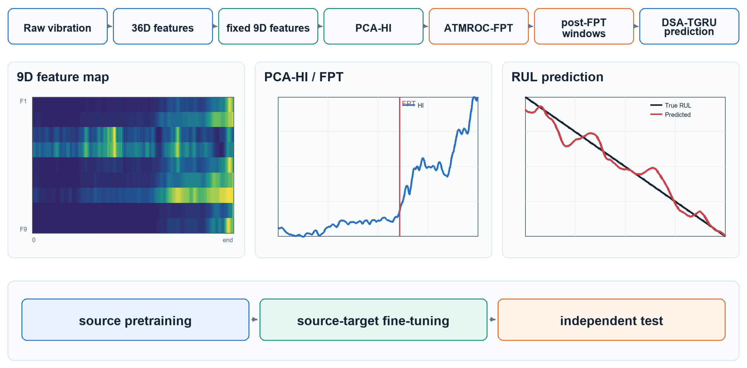
The proposed method consists of six main steps: raw vibration-signal feature extraction, feature selection and health-indicator construction, degradation-start identification, degradation-window sample construction, DSA-TGRU model training, and cross-condition RUL prediction. The overall workflow is shown in Figure 1. First, time-domain, frequency-domain, and time-frequency-domain features are extracted from full-life vibration signals of rolling bearings to obtain multidimensional degradation sequences. The features are then smoothed, normalized, directionally aligned, and reduced to nine degradation-sensitive input features. Next, PCA is used to construct a health indicator, and the ATMROC method is applied to identify the FPT. Finally, RUL labels are constructed from post-FPT windows, and the Transformer-GRU prediction model is trained by source-domain pretraining and target-domain fine-tuning.

2.1. Datasets and Raw Signal Processing

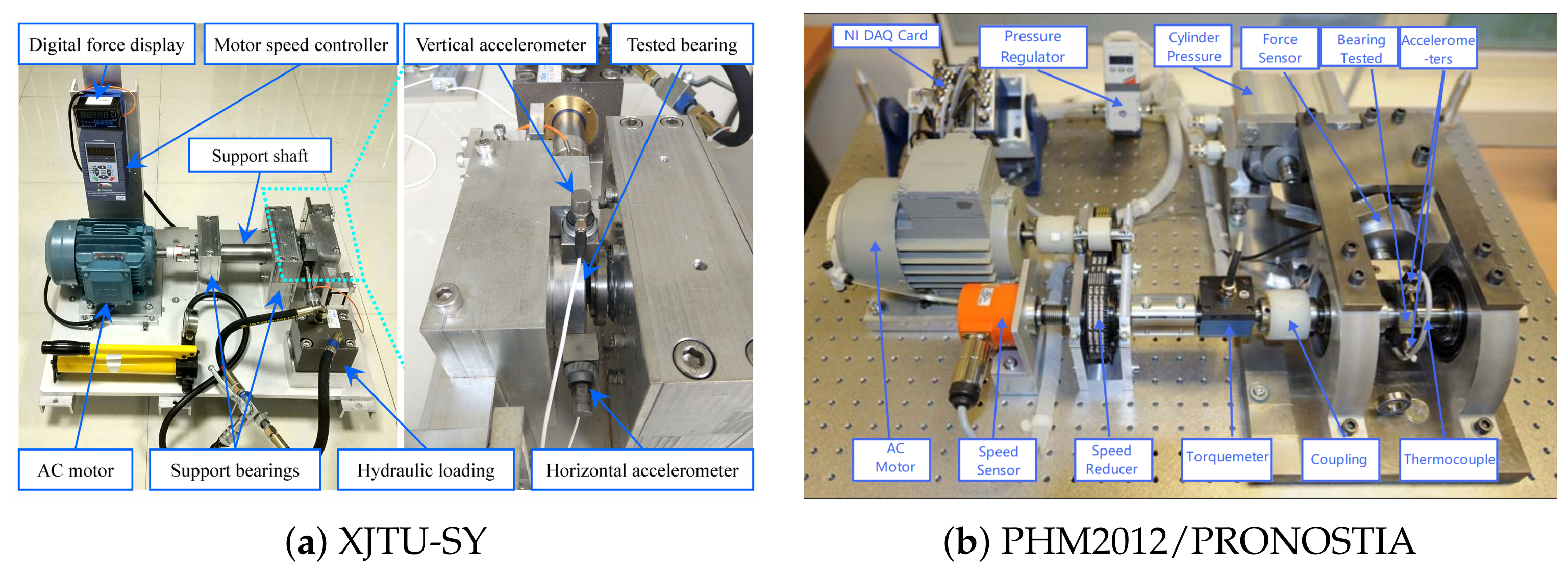
Two public rolling bearing accelerated-life datasets are used in this study [26,27]. The XJTU-SY dataset uses LDK UER204 rolling bearings, whereas the PHM2012/PRONOSTIA dataset uses NSK 6804DD ball bearings. The XJTU-SY dataset was released by Xi’an Jiaotong University (Xi’an, China), and the PHM2012/PRONOSTIA platform was developed by FEMTO-ST Institute (Besancon, France). The public dataset descriptions report LDK UER204 and NSK 6804DD bearings. The first is XJTU-SY, which was collected from an accelerated bearing test rig under different loads and rotational speeds. The sampling frequency is 25.6 kHz, and each sampling file contains 1.28 s of horizontal and vertical vibration signals recorded every 1 min. The second is PHM2012, which was obtained from the PRONOSTIA platform and contains full-life bearing degradation signals under multiple operating conditions. The sampling frequency is also 25.6 kHz, and each file records 0.1 s of vibration signal every 10 s. The test-rig illustrations used in this paper are adapted and relabeled from the corresponding public dataset materials, as shown in Figure 2. The operating conditions are summarized in

Table 1. Operating conditions and sampling settings of the two datasets. H/V denotes horizontal and vertical vibration channels.

Dataset	Cond.	Speed	Load	Sampling
XJTU-SY	C1	2100 r/min (35 Hz)	12 kN	25.6 kHz; 1.28 s/1 min; H/V
	C2	2250 r/min (37.5 Hz)	11 kN	25.6 kHz; 1.28 s/1 min; H/V
	C3	2400 r/min (40 Hz)	10 kN	25.6 kHz; 1.28 s/1 min; H/V
PHM2012	C1	1800 r/min	4000 N	25.6 kHz; 0.1 s/10 s; H/V
	C2	1650 r/min	4200 N	25.6 kHz; 0.1 s/10 s; H/V
	C3	1500 r/min	5000 N	25.6 kHz; 0.1 s/10 s; H/V

.

2.2. Extraction of 36 Degradation Features

To obtain feature representations that reflect bearing degradation states, 36 basic features are extracted from each sampling segment, including 16 time-domain features, 12 frequency-domain features, and 8 time-frequency-domain features. Let a sampling segment be $x=\{x_1,x_2,\dots ,x_N\}$, where N is the number of sampling points. Time-domain features describe the amplitude distribution and impact characteristics of vibration signals, including mean, standard deviation, mean square value, root mean square, maximum, minimum, peak value, peak-to-peak value, mean absolute amplitude, square-root amplitude, skewness, kurtosis, shape factor, crest factor, impulse factor, and margin factor. Typical time-domain features are defined as

$$x_{\mathrm{rms}}=\sqrt{{\displaystyle \frac{1}{N}}\sum _{i=1}^N{x}_i^2},$$

(1)

$$K={\displaystyle \frac{1}{N}}{\displaystyle \sum _{i=1}^N}{\left({\displaystyle \frac{x_i-\overline{x}}{\sigma }}\right)}^4,$$

(2)

where $x_{\mathrm{rms}}$ is the root mean square, K is the kurtosis, and $\overline{x}$ and $\sigma$ are the signal mean and standard deviation, respectively. As local bearing damage develops, impact components increase, and features such as peak value, kurtosis, impulse factor, and margin factor usually change significantly.

Frequency-domain features describe the distribution of vibration energy along the frequency axis. A fast Fourier transform is first applied to each signal segment to obtain the amplitude spectrum $s_k$ and the corresponding frequency $f_k$. Then, 12 spectral statistics are calculated, including spectral mean, spectral variance, spectral skewness, spectral kurtosis, frequency centroid, frequency standard deviation, root mean square frequency, and several spectral shape factors. The frequency centroid is defined as

$$f_c={\displaystyle \frac{{\sum }_{k=1}^M{f}_k{s}_k}{{\sum }_{k=1}^M{s}_k}},$$

(3)

where M is the number of spectral points. Frequency-domain features reflect spectral energy migration and frequency-band distribution changes caused by fault impacts.

Time-frequency-domain features describe energy variations of nonstationary vibration signals in different frequency bands. A three-level wavelet packet decomposition is applied to each sampling segment to obtain eight terminal sub-bands, and the wavelet-packet energy of each sub-band is calculated as

$$E_j={\displaystyle \sum _{n=1}^{L_j}}{c}_{j,n}^2,j=1,2,\dots ,8,$$

(4)

where $c_{j,n}$ is the wavelet-packet coefficient in the jth sub-band, and $L_j$ is the coefficient length of that sub-band. The 16 time-domain, 12 frequency-domain, and 8 time-frequency-domain features are concatenated to form a 36-dimensional basic degradation feature vector for each sampling instant.

2.3. Feature Preprocessing and Nine-Dimensional Feature Selection

Because different features have different physical units and value ranges, directly feeding them into the prediction model may cause large-amplitude features to dominate model training. Therefore, Savitzky–Golay smoothing, Min–Max normalization, and directional alignment are applied to the extracted features. For the jth feature, Min–Max normalization is defined as

$$z_{i,j}=\left\{\begin{array}{cc}{\displaystyle \frac{x_{i,j}-x_j^{min}}{x_j^{max}-x_j^{min}}},\hfill & x_j^{max}>x_j^{min},\hfill \\ 0,\hfill & x_j^{max}=x_j^{min},\hfill \end{array}\right.$$

(5)

where $x_{i,j}$ is the jth feature at the ith sampling instant, and $x_j^{min}$ and $x_j^{max}$ are the minimum and maximum values of that feature over the current bearing full-life sequence. Directional alignment aims to make features increase with degradation. If the initial value of a normalized feature is larger than its terminal value, it is transformed into $1-z_{i,j}$. It should be emphasized that this paper adopts an offline full-life retrospective analysis protocol. The full-life Min–Max scale of the current bearing is used for offline feature-scale unification, HI construction, and retrospective representation of the test-bearing degradation trajectory. Full-life normalization is not used to provide RUL labels or failure-time information to the prediction model, and the test bearing is not used for model parameter updating or model selection. However, the global feature range may include late-degradation or near-failure observations and may therefore introduce future scale information through feature scaling. Thus, this preprocessing should be interpreted as an offline retrospective protocol rather than an online prediction protocol. For a fixed Min–Max scaler, the most stable scale is one whose lower and upper bounds cover the expected feature ranges of both source and target operating scenarios as fully as possible. If the scale is estimated only from offline source-domain bearings, the possible target-domain feature range should be anticipated from historical records, engineering calibration data, healthy baselines, or limited target-domain records available under the offline protocol. When the source-domain range is much narrower than, or shifted from, the target-domain range, clipping target or test observations to $[0,1]$ can cause boundary saturation and range compression, thereby introducing an additional distribution shift. Therefore, for online deployment, the normalization scale should be determined from source-domain training bearings, historical healthy baselines, recursively updated windows, or calibrated ranges that reasonably cover the expected target-domain feature amplitudes.

After obtaining the 36 normalized features, this paper does not feed all features directly into the model. Instead, a fixed candidate feature set covering time-domain, frequency-domain, and time-frequency-domain information is first constructed. Specifically, a predefined degradation-sensitive feature list is used to select 10 candidate features from the 36 features. Then, based on trendability, monotonicity, and stability evaluations on source-domain training bearings, the sixth unstable feature in the 10-dimensional candidate set is fixedly removed, resulting in nine input features. The fixed candidate-feature selection is summarized in

Table 2. Fixed selection of the final nine input features.

Dataset	10 Candidates	Drop	Final Inputs
XJTU-SY	$T6$, $T10$, $T12$, $T13$, $T16$, $F3$, $F10$, $F11$, $A0$, $A1$	$F3$	$T6$, $T10$, $T12$, $T13$, $T16$, $F10$, $F11$, $A0$, $A1$
PHM2012	Std, RMS, Max, P2P, MAA, Kurt., $F1$, $F2$, $F6$, Band-1 energy	Kurt.	Std, RMS, Max, P2P, MAA, $F1$, $F2$, $F6$, Band-1 energy

Note: For XJTU-SY, $T6$, $T10$, $T12$, $T13$, and $T16$ denote minimum, square-root amplitude, kurtosis, shape factor, and margin factor; $F3$, $F10$, and $F11$ denote spectral-amplitude skewness, frequency dispersion coefficient, and spectral skewness; $A0$ and $A1$ denote the first two wavelet-packet band energies. For PHM2012, Std, RMS, Max, P2P, MAA, and Kurt denote standard deviation, root mean square, maximum, peak-to-peak value, mean absolute amplitude, and kurtosis, respectively.

. This rule is determined before all tasks and remains unchanged during HI construction, degradation-start identification, and model training. It is not adjusted according to target test bearings or experimental results, reducing the risk of manual tuning or test-result-oriented feature selection.

Feature evaluation is performed only on source-domain training bearings. Let the normalized sequence of a candidate feature be ${\mathbf{z}}_j=\{z_{1,j},z_{2,j},\dots ,z_{T,j}\}$. Its trendability, monotonicity, and stability are evaluated as follows:

$${\mathrm{Trend}}_j=\left|\mathrm{corr}({\mathbf{z}}_j,\mathbf{t})\right|,$$

(6)

$${\mathrm{Mono}}_j=\left|{\displaystyle \frac{N_{+}-N_{-}}{T-1}}\right|,N_{+}={\displaystyle \sum _{t=2}^T}\mathbb{I}(z_{t,j}-z_{t-1,j}\ge 0),N_{-}={\displaystyle \sum _{t=2}^T}\mathbb{I}(z_{t,j}-z_{t-1,j}<0),$$

(7)

$${\mathrm{Stab}}_j={\displaystyle \frac{1}{1+\mathrm{std}(∆z_j)}},∆z_j={\{z_{t,j}-z_{t-1,j}\}}_{t=2}^T.$$

(8)

Here, $\mathbf{t}=\{1,2,\dots ,T\}$ is the time index, and $\mathbb{I}(·)$ is the indicator function. A higher trendability indicates stronger correlation with lifetime progression; a higher monotonicity indicates a more consistent increasing or decreasing direction; and a higher stability indicates smaller local incremental fluctuation. The sixth candidate feature is removed according to the combined behavior of these three indicators on source-domain training bearings, without using target test-bearing prediction errors to adjust the feature set.

The final nine features still include amplitude statistics, impact-sensitive features, spectral-shape features, and time-frequency energy features. Time-domain features reflect vibration amplitude and impact intensity, frequency-domain features describe spectral energy distribution and frequency structure, and time-frequency-domain features characterize local band-energy changes in nonstationary degradation. Compared with using all 36 features, the fixed selection scheme reduces the influence of redundant dimensions and unstable features on PCA-HI, ATMROC degradation-start identification, and subsequent Transformer-GRU training.

2.4. PCA-HI Construction

To compress multidimensional degradation features into a one-dimensional indicator describing bearing health-state evolution, the nine selected features of each bearing are normalized column-wise, and principal component analysis is used to extract the first principal component as the initial health indicator. Health-indicator construction is a common step in bearing degradation monitoring and RUL prediction. Previous studies have constructed health representations using recurrent neural networks, sparse autoencoders, state-space modeling, and entropy features [8,28,29]. The PCA-HI construction in this paper is also an offline full-life retrospective step. It uses the complete degradation trajectory to determine the HI scale and degradation start and is not treated as directly available information for online prediction. Let the normalized nine-dimensional feature matrix be $\mathbf{X}\in {\mathbb{R}}^{T\times 9}$. PCA projects the centered feature matrix onto the maximum-variance direction:

$${\mathrm{PC}}_1\left(t\right)=({\mathbf{x}}_t-\mathit{\mu }){\mathbf{w}}_1,$$

(9)

where ${\mathbf{x}}_t$ is the feature vector at the tth sampling instant, $\mathit{\mu }$ is the mean vector of the current bearing feature sequence, and ${\mathbf{w}}_1$ is the first principal-component direction. Then, ${\mathrm{PC}}_1\left(t\right)$ is robustly Min–Max normalized to obtain ${\mathrm{HI}}_{\mathrm{raw}}\left(t\right)$. Smoothing and directional alignment are further applied so that the final $\mathrm{HI}\left(t\right)$ generally increases with degradation and is constrained to the interval $[0,1]$. This indicator is used for degradation-start identification.

It should be noted that PCA-HI mainly serves as an auxiliary degradation indicator in this paper. It is used for FPT identification, RUL label construction, and degradation-process visualization, whereas the main prediction model still uses the nine selected features as inputs. This is because HI compresses nine features into one comprehensive indicator that highlights the overall degradation trend but may lose local impact, spectral-shape, and time-frequency energy details. Moreover, the HI construction in this paper depends on offline full-life retrospective analysis. Directly using HI as a model input would further increase the dependence of prediction on complete offline degradation trajectories. To analyze the effect of using HI as a prediction input, Section 3.8.3 reports HI-only and nine-feature-plus-HI input comparison experiments.

2.5. ATMROC-Based Degradation-Start Identification

Rolling bearings are usually relatively stable in the early healthy stage. If full-life samples are directly used for model training, healthy-stage samples may obscure key degradation-stage changes. Degradation-start identification is related to changepoint detection [30]. In bearing prognostics, degradation-boundary or stage-aware modeling has also been used to support label construction and prediction-model training [7,31]. Therefore, this paper uses an adaptive threshold moving rate of change (ATMROC) method to identify the bearing degradation start. For the smoothed health indicator $\mathrm{HI}\left(t\right)$, the forward moving rate of change is defined as

$$\mathrm{ROC}\left(t\right)={\displaystyle \frac{max(0,\mathrm{HI}(t+w)-\mathrm{HI}(t\left)\right)}{w}},$$

(10)

where w is the moving-window length. In this paper, $w=32$. The threshold is determined jointly by the mean, standard deviation, and median absolute deviation (MAD) of the early healthy-stage ROC:

$$\theta =max({\mu }_{\mathrm{ROC}}+\lambda {\sigma }_{\mathrm{ROC}},{\mathrm{median}}_{\mathrm{ROC}}+6\times 1.4826\times {\mathrm{MAD}}_{\mathrm{ROC}},{\theta }_{min}),$$

(11)

where $\lambda =2.0$, and ${\theta }_{min}$ is the minimum threshold. If the ROC continuously exceeds the threshold after a certain time and the window-end HI has left the healthy plateau, a clear degradation trend is considered to have appeared. The FPT $t_{\mathrm{FPT}}$ is then determined within the triggered window according to HI increment or HI-level confirmation conditions and is used as the boundary for RUL label construction and training-sample filtering. The ATMROC parameters are listed in

Table 3. ATMROC parameters for degradation-start identification.

Parameter	Common Setting	XJTU-SY	PHM2012
w	32	–	–
$\lambda$	2.0	–	–
Healthy baseline	First 20%; 20–100 ROC windows	–	–
${\theta }_{min}$	0.001	–	–
HI plateau bound	–	$max({\overline{h}}_0+4{\sigma }_{h,0},0.12)$	$max({\overline{h}}_0+4{\sigma }_{h,0},0.15)$
Trigger count	–	3 ROC points	5 ROC points
Confirmation	–	Future HI increase $>0.08$	Above plateau for $max(5,\mathrm{round}(0.01T\left)\right)$ points
FPT localization	–	Triggered window; 60%/45% HI rise	Later of persistent ROC trigger and HI departure

.

2.6. Degradation-Window Sample Construction and RUL Labels

After identifying the degradation start, the FPT is used as the boundary between the healthy and degradation stages. For a bearing sequence of length T, the sampling index is defined as $t=1,2,\dots ,T$. If the degradation start is $t_{\mathrm{FPT}}$, the complete normalized RUL curve can be defined as

$$y\left(t\right)=\left\{\begin{array}{cc}1,\hfill & t<t_{\mathrm{FPT}},\hfill \\ 1-{\displaystyle \frac{t-t_{\mathrm{FPT}}}{T-t_{\mathrm{FPT}}}},\hfill & t\ge t_{\mathrm{FPT}},\hfill \end{array}\right.$$

(12)

where $y\left(t\right)\in [0,1]$, $y\left(t\right)=1$ denotes the beginning of degradation or the healthy plateau, and $y\left(T\right)=0$ denotes the end of life under the one-based index. It should be emphasized that $y=1$ for $t<t_{\mathrm{FPT}}$ in the equation is used only for complete-lifetime curve illustration and visualization. Model training and test evaluation are based only on post-FPT windows, and healthy-stage windows do not contribute to the loss. A sliding-window form is used to construct model inputs, with the window length set to 25. For each window, the RUL at the window-end instant is used as the window label. If the window end is earlier than the FPT, the window is excluded from training and evaluation. This strategy focuses model training on the degradation stage and reduces interference from stationary healthy-stage samples.

2.7. DSA-TGRU Prediction Model

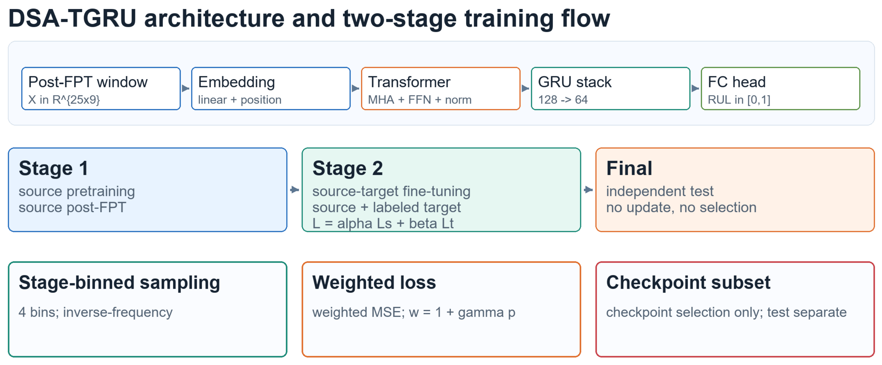
The proposed DSA-TGRU model consists of an input embedding layer, a Transformer encoder, two GRU layers, and a fully connected regression head. The network structure is shown in Figure 3.

Given an input window ${\mathbf{X}}_t\in {\mathbb{R}}^{L\times d}$, where $L=25$ is the window length and $d=9$ is the input feature dimension, a linear mapping projects the input features into a hidden dimension, and positional encoding is added to preserve temporal order:

$${\mathbf{H}}_0={\mathbf{X}}_t{\mathbf{W}}_e+{\mathbf{b}}_e+\mathbf{P}.$$

(13)

Transformer-based feature modeling has been used in RUL prediction [24], while recurrent neural-network structures are suitable for degradation-sequence and health-indicator modeling [8,19]. Therefore, this paper combines a Transformer encoder and GRU layers to model both global dependencies and recurrent temporal evolution. The Transformer encoder uses multi-head self-attention to capture long-range dependencies among different time steps within the window, generating a high-level temporal representation ${\mathbf{H}}_{\mathrm{tr}}$. Two GRU layers further model the temporal evolution of degradation. The hidden state of the last time step is used as the window-level degradation representation:

$${\mathbf{h}}_{\mathrm{gru}}=\mathrm{GRU}{\left({\mathbf{H}}_{\mathrm{tr}}\right)}_L.$$

(14)

Finally, the fully connected regression head outputs the normalized RUL prediction:

$$\widehat{y}=f_{\mathrm{fc}}\left({\mathbf{h}}_{\mathrm{gru}}\right).$$

(15)

The Transformer captures global associations in degradation sequences, whereas the GRU preserves recurrent temporal-evolution characteristics. Their combination enhances representation of complex degradation processes.

2.8. Source-Domain Pretraining, Target-Domain Fine-Tuning, and Stage-Aware Training

To improve cross-condition generalization, the model is trained using source-domain pretraining followed by target-domain fine-tuning. The experimental protocol is offline target-domain fine-tuning with limited labeled samples: post-FPT windows and RUL labels from a small number of target-domain run-to-failure bearings are used for fine-tuning, and a target-domain checkpoint-selection subset (hereafter, checkpoint subset) is used to record error changes. The checkpoint metric is computed on data drawn from the target-domain fine-tuning bearings and is used to select the retained checkpoint. Because it is not based on a fully independent target-domain bearing, this design may introduce optimistic model-selection bias. The test bearing is not used for parameter updating or model selection, and final performance is reported only on the independent test bearing.

Let the source-domain training set be ${\mathcal{D}}_s$ and the target-domain fine-tuning set be ${\mathcal{D}}_t$. The model is first pretrained for 200 epochs on source-domain samples to learn general degradation representations. It is then fine-tuned for 100 epochs using both source- and target-domain samples, with the learning rate reduced to 0.1 times the pretraining learning rate. The fine-tuning loss is

$$\mathcal{L}=\alpha {\mathcal{L}}_s+\beta {\mathcal{L}}_t,$$

(16)

where ${\mathcal{L}}_s$ and ${\mathcal{L}}_t$ are weighted mean squared errors on labeled source- and target-domain post-FPT windows, respectively. The weights are $\alpha =1.0$ and $\beta =0.1$. Therefore, the proposed method does not claim to perform transfer without any target labels. It targets engineering scenarios where a small number of offline labeled target-domain degradation samples are available.

To increase attention to rapid late-life degradation, a late-stage linear weighting term is introduced into the loss. Let the sample degradation progress be $p=1-y$. The sample weight is defined as

$$\omega =1+\gamma p,$$

(17)

where $\gamma =0.5$. The corresponding weighted mean squared error is

$${\mathcal{L}}_{\mathrm{wmse}}={\displaystyle \frac{{\sum }_i{\omega }_i{({\widehat{y}}_i-y_i)}^2}{{\sum }_i{\omega }_i}}.$$

(18)

In addition, stage-binned sampling is introduced by dividing degradation progress into four bins and applying inverse-frequency stage-weighted sampling to alleviate sample imbalance among degradation stages.

2.9. Evaluation Metrics

MAE, MSE, and RMSE are used to evaluate prediction performance. Let the test set contain n post-FPT test windows, with true RUL $y_i$ and predicted RUL ${\widehat{y}}_i$. The metrics are defined as

$$\mathrm{MAE}={\displaystyle \frac{1}{n}}{\displaystyle \sum _{i=1}^n}|{\widehat{y}}_i-y_i|,$$

(19)

$$\mathrm{MSE}={\displaystyle \frac{1}{n}}{\displaystyle \sum _{i=1}^n}{({\widehat{y}}_i-y_i)}^2,$$

(20)

$$\mathrm{RMSE}=\sqrt{{\displaystyle \frac{1}{n}}\sum _{i=1}^n{({\widehat{y}}_i-y_i)}^2}.$$

(21)

Lower MAE and RMSE indicate lower prediction error. In addition to normalized errors, this paper reports absolute errors, denoted as Abs. MAE and Abs. RMSE. They are calculated by multiplying the normalized error by the effective length from FPT to end of life for the test bearing. Their unit is the number of post-FPT sampling segments. These absolute errors are not measured in minutes or seconds but in sampling-segment counts consistent with dataset file sequences. To reduce the influence of random initialization, each experiment is repeated using five random seeds, and the mean and standard deviation are reported.

The feature-preprocessing settings and DSA-TGRU training settings are summarized in

Table 4. Feature preprocessing settings.

Item	XJTU-SY	PHM2012
Channel	Horizontal	Horizontal (h)
Segment length	32,768 → 2048 points	2560 points
Frequency for FFT	25,600 Hz	25,600 Hz
Wavelet denoising	db4; 3 levels; soft threshold	db4; 5 levels; soft threshold
Wavelet-packet energy	db5; 3 levels; 8 bands	db5; 3 levels; 8 bands
Smoothing	SG window 19; order 3	SG window 29; order 3
Input dimension	9 features	9 features

and

Table 5. DSA-TGRU training settings.

Item	Setting
Input	Window length 25; 9 features
Random seeds	0, 1, 2, 3, and 4
Epochs	200 source pretraining + 100 target fine-tuning
Optimizer/LR	Adam; $3\times {10}^{-4}$ pretraining; $3\times {10}^{-5}$ fine-tuning
Batch size	32 for training; 128 for evaluation
Transformer	Hidden 32; 4 heads; 1 layer; $q=v=8$; attention size 12; dropout 0.1
GRU/head	Two GRU layers (128, 64); last time step to regression head
Stage handling	4 post-FPT bins; inverse-frequency stage sampling
Loss weights	$\alpha =1.0$, $\beta =0.1$, $\gamma =0.5$
Checkpoint selection	No early stopping; checkpoint selected by lowest checkpoint-subset MAE; clipping 10.0
Data loading	num_workers = 0

, respectively. The computational workflow was implemented using Python 3.9.25, PyTorch 2.5.1, NumPy 1.26.4, SciPy 1.13.1, scikit-learn 1.5.1, PyWavelets 1.6.0, pandas 2.3.3, and Matplotlib 3.9.4.

3. Results

This section verifies the proposed method on the XJTU-SY and PHM2012 rolling bearing datasets. The results include degradation-feature visualization, degradation-start identification, cross-condition RUL prediction, normalization-protocol sensitivity analysis, comparison with transfer prediction baselines, transfer-contribution controls, model-structure and training-strategy ablation experiments, HI input comparison, and stability and significance analysis. Unless otherwise stated, table results are averaged over five random seeds, and the standard deviations in the main prediction table indicate fluctuations under different random seeds.

3.1. Experimental Task Settings

To clarify the relationships among target-domain fine-tuning, checkpoint selection, and test samples,

Table 6. Cross-condition task splits. Src., Tgt., Chk., and Test denote source pretraining, target fine-tuning, checkpoint subset, and independent test bearings, respectively. B1_1 denotes Bearing1_1, B2_3 denotes Bearing2_3, and so forth.

Dataset	Task	Cond.	Src.	Tgt.	Chk.	Test
XJTU-SY	t1	C1 → C2	B1_1, B1_2, B1_3	B2_2, B2_5	B2_5	B2_3
	t2	C1 → C2	B1_1, B1_2, B1_3	B2_2, B2_3	B2_3	B2_5
	t3	C2 → C1	B2_2, B2_3, B2_5	B1_1, B1_2	B1_2	B1_3
PHM2012	t1	C1 → C2	B1_1, B1_3	B2_4	B2_4	B2_1
	t2	C2 → C1	B2_1, B2_4	B1_3	B1_3	B1_4
	t3	C2 → C1	B2_1, B2_4	B1_4	B1_4	B1_3

lists the cross-condition task splits used in this paper. Source-domain bearings are used for pretraining. Target-domain fine-tuning bearings are used for offline target-domain fine-tuning. The checkpoint metric is computed on data drawn from the target-domain fine-tuning bearings and is used to select the retained checkpoint. The test bearing is used only for final performance evaluation and does not participate in parameter updating or model selection.

All tasks are trained and evaluated independently. Different tasks do not share model parameters, model-selection results, or test-bearing information. The checkpoint metric is computed on data drawn from the target-domain fine-tuning bearings and is used to select the retained checkpoint. Because it is not based on a fully independent target-domain bearing, this design may introduce optimistic model-selection bias, especially when only one target-domain run-to-failure bearing is available. Final performance is reported only on the independent test bearing. For bearings whose roles change across different tasks, such as Bearing2_3 and Bearing2_5 in XJTU-SY, data are used only according to the role specified in Table 6 for the corresponding task. The test bearing in a task does not participate in parameter updating or model selection for that task.

3.2. Visualization of Degradation Features

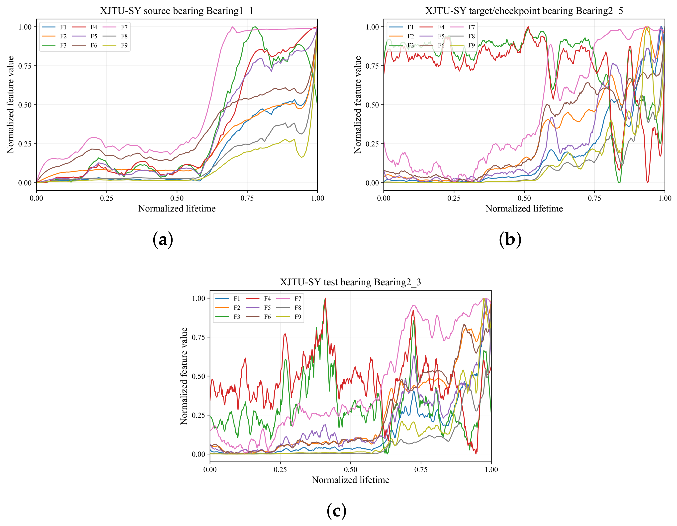
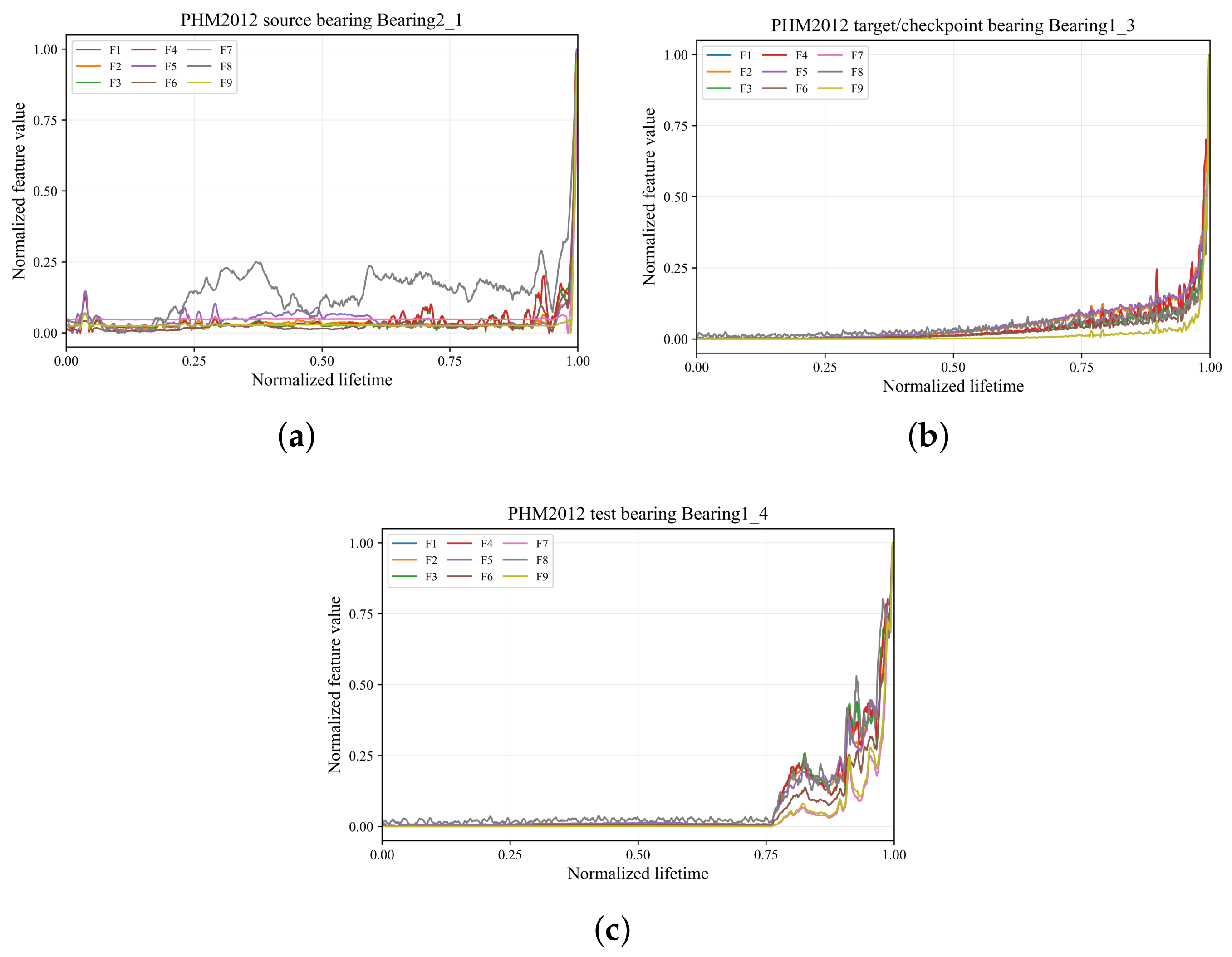
To show the change trends of the selected nine features in cross-condition tasks, one representative task from each dataset is selected. Feature curves are shown for source-domain bearings, target-domain fine-tuning/checkpoint bearings, and test bearings. Figure 4 shows an example from the XJTU-SY C1 → C2 task, where Bearing1_1 is a source-domain bearing, Bearing2_5 is used for target-domain fine-tuning and checkpoint selection, and Bearing2_3 is the test bearing. The source- and target-domain bearings differ in degradation speed, feature fluctuation amplitude, and late-stage impact enhancement, which explains why cross-condition RUL prediction requires transfer learning and target-domain fine-tuning.

Figure 5 shows an example from the PHM2012 C2 → C1 task, where Bearing2_1 is a source-domain bearing, Bearing1_3 is used for target-domain fine-tuning and checkpoint selection, and Bearing1_4 is the test bearing. Compared with XJTU-SY, some PHM2012 bearings show obvious degradation later, and the feature amplitudes and fluctuation patterns differ more strongly among bearings. This is consistent with the higher prediction errors observed for PHM2012 in later experiments.

3.3. Degradation-Start Identification Results

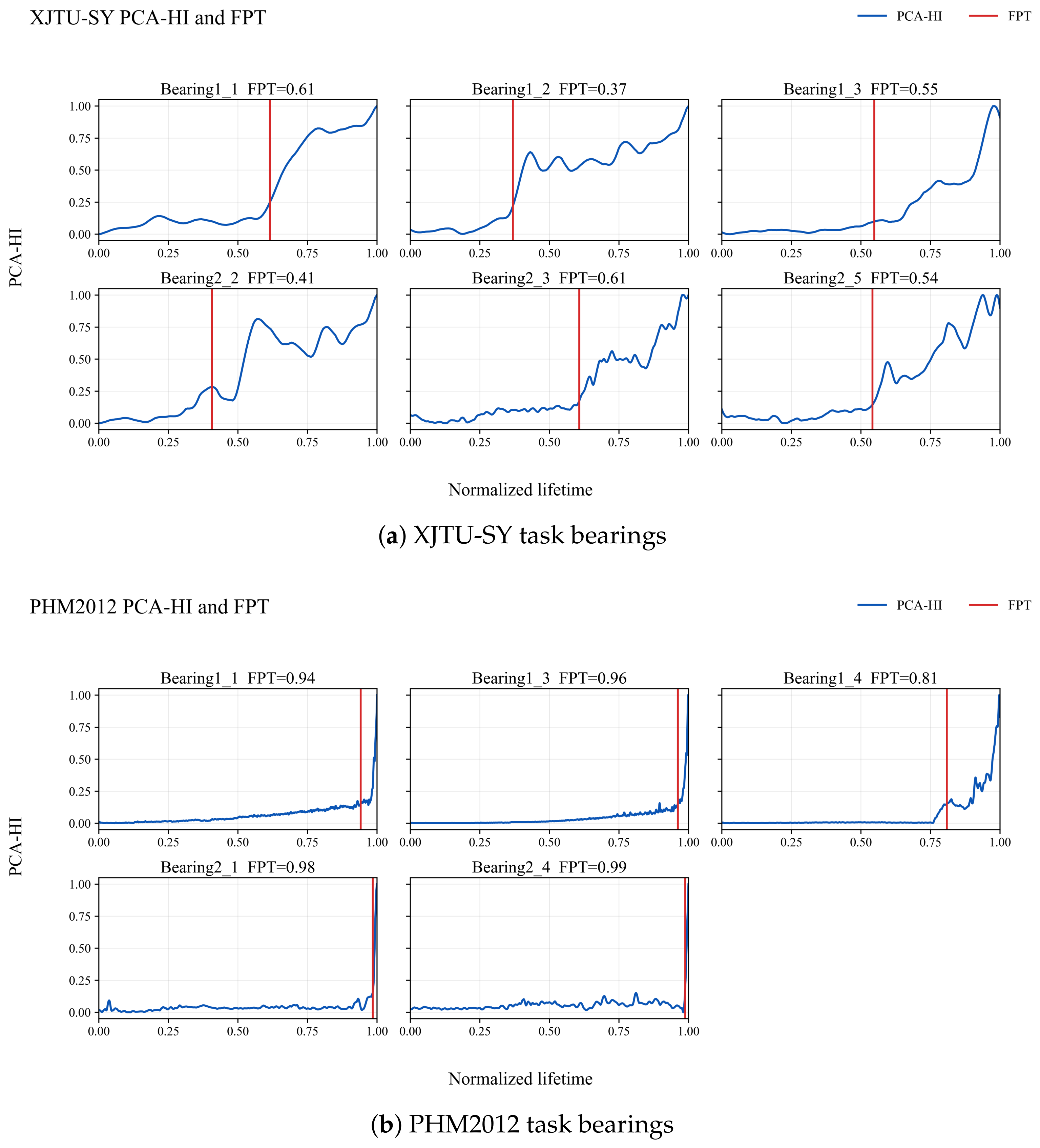
The PCA-HI and ATMROC results show that the proposed procedure can provide clear degradation-stage boundaries for subsequent RUL label construction. In the XJTU-SY dataset, 15 bearings are processed, of which 12 obtain valid degradation points from the consecutive ROC triggering condition. The average degradation-start ratio is 0.657, indicating that most bearings enter an obvious degradation stage in the middle-to-late lifetime. In the PHM2012 dataset, 16 bearings are processed, and 13 satisfy the valid triggering condition. The average degradation-start ratio is 0.882, indicating that the obvious degradation process in this dataset is more concentrated near the end of life. The FPT indices of the two datasets are summarized and used during training to construct degradation-stage RUL labels.

In terms of health-indicator quality, the average HI trendability of XJTU-SY is 0.698, and its average late-stage increase is 0.519. For PHM2012, the corresponding values are 0.372 and 0.108. Thus, the PCA-HI degradation trend is clearer in XJTU-SY, whereas some PHM2012 bearings exhibit later and weaker degradation changes, increasing cross-condition prediction difficulty.

Figure 6 shows the FPT identification curves for all bearings involved in the t1–t3 cross-condition task splits of the two datasets.

3.4. Main Cross-Condition Prediction Results

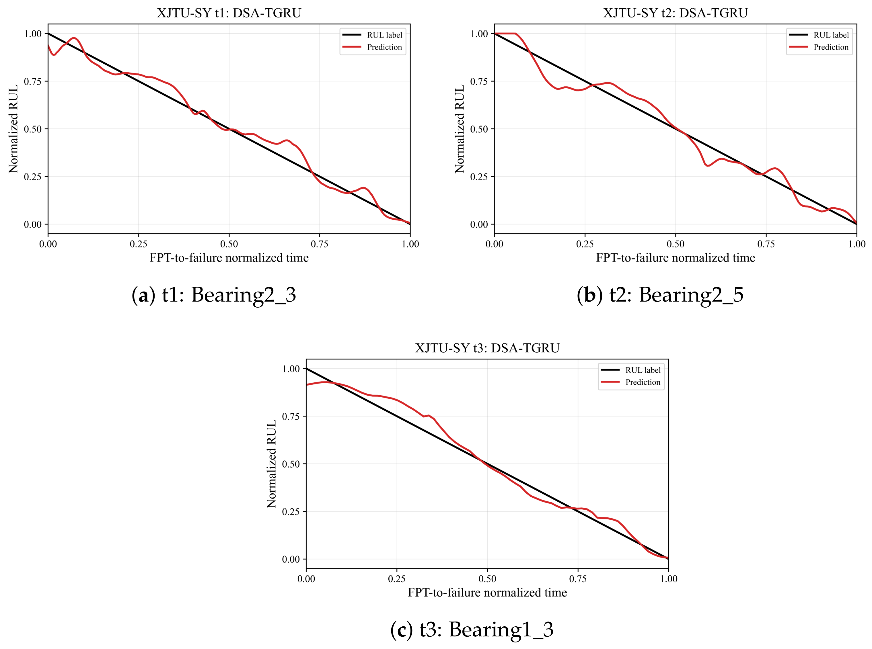
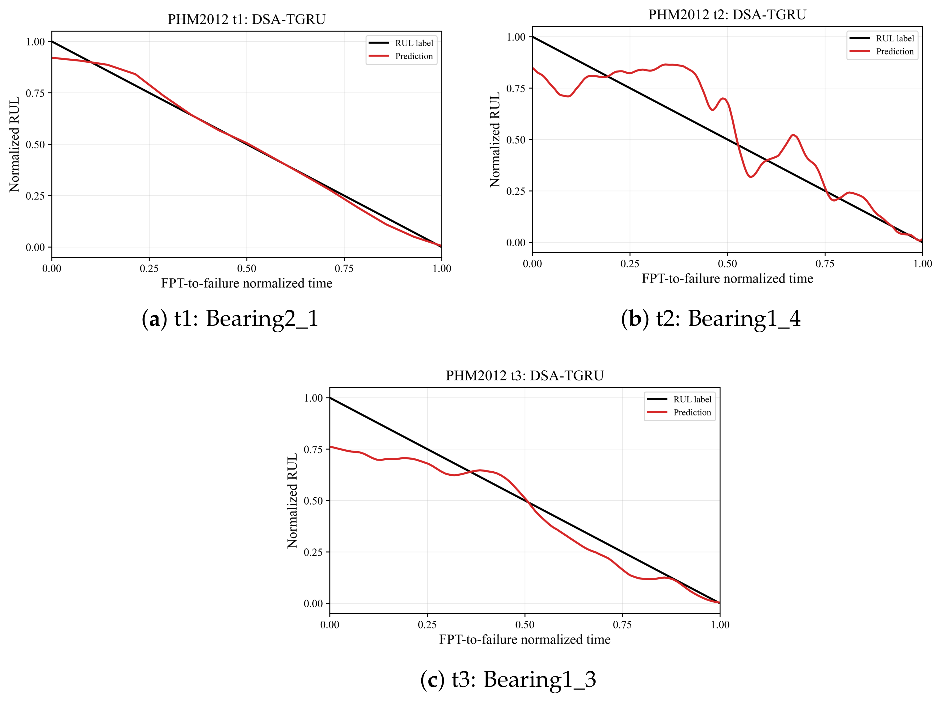
Figure 7 and Figure 8 first show the RUL prediction curves for the t1–t3 tasks on XJTU-SY and PHM2012, respectively. In general, DSA-TGRU follows the decreasing trend of the true RUL. The deviation in PHM2012 task t2 is more obvious and is further reflected by the numerical metrics reported below.

Table 7. Main DSA-TGRU prediction results. Absolute errors are reported in post-FPT sampling segments.

Dataset	Task	Cond.	Test	MAE	RMSE	Abs. MAE	Abs. RMSE
XJTU-SY	t1	C1 → C2	B2_3	0.0466 ± 0.0085	0.0610 ± 0.0138	9.75 ± 1.78	12.74 ± 2.88
	t2	C1 → C2	B2_5	0.0494 ± 0.0082	0.0608 ± 0.0102	7.66 ± 1.28	9.42 ± 1.58
	t3	C2 → C1	B1_3	0.0516 ± 0.0197	0.0662 ± 0.0266	3.66 ± 1.40	4.70 ± 1.89
PHM2012	t1	C1 → C2	B2_1	0.0294 ± 0.0093	0.0388 ± 0.0092	0.41 ± 0.13	0.54 ± 0.13
	t2	C2 → C1	B1_4	0.1104 ± 0.0143	0.1365 ± 0.0131	30.14 ± 3.91	37.26 ± 3.57
	t3	C2 → C1	B1_3	0.0814 ± 0.0068	0.1031 ± 0.0084	7.41 ± 0.62	9.39 ± 0.76

reports the corresponding numerical results of DSA-TGRU on the two datasets.

XJTU-SY contains three cross-condition tasks, with an average MAE of 0.0492 and an average RMSE of 0.0626. PHM2012 also contains three cross-condition tasks, with an average MAE of 0.0738 and an average RMSE of 0.0928. Overall, the model yields lower prediction errors on XJTU-SY, and the MAE values of the three tasks remain between 0.0466 and 0.0516. For PHM2012, the error of task t2 is relatively high, mainly because the FPT of the test bearing is later, the effective post-FPT degradation segment is shorter, and the PCA-HI trendability is weaker than that of XJTU-SY. Consequently, the target-domain fine-tuning stage has less usable degradation information.

3.5. Normalization-Protocol Sensitivity Analysis

The main experiments use full-life Min–Max normalization under the offline retrospective protocol described in Section 2.3. This operation does not provide RUL labels or failure-time information to the prediction model, but the minimum and maximum values of a full run-to-failure trajectory may include late-degradation or near-failure observations and may affect the scaled feature distribution. Therefore, an additional control experiment is conducted to evaluate sensitivity to the normalization protocol. This experiment is used to quantify protocol sensitivity; it is not intended to prove that the original model performance depends on information leakage.

In the control setting, for each transfer task, the Min–Max statistics of each feature are fitted only on the source-domain bearings. The same source-domain statistics are then applied to the source-domain training bearings, target-domain fine-tuning bearings, checkpoint subset, and test bearing. Values outside the source-domain range are clipped to $[0,1]$. This stricter protocol avoids using target or test full-life extrema to estimate feature scales, but it should be interpreted as a conservative reference rather than an automatically optimal normalization choice. In cross-condition prediction, a Min–Max range that covers both source and target operating scenarios is generally more suitable for stable feature scaling. When only source-domain offline statistics are used, the possible target-domain Min–Max range should be estimated as far as possible; otherwise, target/test observations outside the source range may be clipped to the interval boundaries, which avoids extrapolated normalized values but also causes boundary saturation, range compression, and a shifted feature distribution.

Table 8. Normalization-protocol sensitivity control results. Source-domain Min–Max uses only source-domain feature ranges for scaling, followed by clipping to $[0,1]$. $∆$ denotes source-domain Min–Max minus full-life Min–Max.

Dataset	Task	Full-Life MAE	Source-Domain MAE	∆MAE	Full-Life RMSE	Source-Domain RMSE	∆RMSE
XJTU-SY	t1	0.0466 ± 0.0085	0.1546 ± 0.0365	+0.1079	0.0610 ± 0.0138	0.1967 ± 0.0427	+0.1357
	t2	0.0494 ± 0.0082	0.2640 ± 0.0715	+0.2145	0.0608 ± 0.0102	0.3188 ± 0.0896	+0.2581
	t3	0.0516 ± 0.0197	0.2251 ± 0.0261	+0.1735	0.0662 ± 0.0266	0.2504 ± 0.0223	+0.1842
	Avg.	0.0492 ± 0.0125	0.2146 ± 0.0651	+0.1653	0.0626 ± 0.0171	0.2553 ± 0.0751	+0.1927
PHM2012	t1	0.0294 ± 0.0093	0.0924 ± 0.0188	+0.0630	0.0388 ± 0.0092	0.1105 ± 0.0184	+0.0717
	t2	0.1104 ± 0.0143	0.1562 ± 0.0064	+0.0458	0.1365 ± 0.0131	0.1838 ± 0.0076	+0.0473
	t3	0.0814 ± 0.0068	0.1320 ± 0.0169	+0.0506	0.1031 ± 0.0084	0.1524 ± 0.0174	+0.0492
	Avg.	0.0738 ± 0.0360	0.1269 ± 0.0306	+0.0531	0.0928 ± 0.0431	0.1489 ± 0.0341	+0.0561

shows that the normalization protocol has a clear influence on cross-condition prediction performance. Under source-domain Min–Max normalization, the average MAE/RMSE increase from 0.0492/0.0626 to 0.2146/0.2553 on XJTU-SY and from 0.0738/0.0928 to 0.1269/0.1489 on PHM2012. The larger degradation on XJTU-SY indicates that the source-domain ranges do not sufficiently cover the target/test feature amplitudes in some tasks, so the normalized features can suffer from clipping-induced saturation and cross-condition distribution shift. These results do not by themselves prove that the full-life protocol is the sole reason for the main-result performance; they show that cross-condition RUL prediction is sensitive to feature-scaling assumptions and range-coverage mismatch. Accordingly, the main results should be interpreted as offline full-life retrospective results. The source-domain normalization results provide a stricter reference protocol for settings where target/test full-life scale information is unavailable, but practical deployment still requires a calibrated normalization range that represents both source and expected target operating scenarios as much as possible.

3.6. Comparison with Other Methods

To further evaluate the proposed method, DSA-TGRU is compared with CADA [32], GSAN [23], TACDA [25], TCNN [33], TDA [24], and WDANN [20]. Source-only and target-only variants are also included as internal controls. Source-only is trained only on source-domain bearings, whereas target-only uses the same Transformer-GRU architecture but is trained from scratch only on target-domain post-FPT windows.

Table 9. Average performance of different methods (mean ± standard deviation). Absolute errors are in post-FPT sampling segments.

Dataset	Method	MAE	RMSE	Abs. MAE	Abs. RMSE
XJTU-SY	Source-only	0.2866 ± 0.0949	0.3346 ± 0.1193	43.57 ± 22.84	51.07 ± 27.36
	Target-only	0.1671 ± 0.1066	0.1910 ± 0.1144	19.08 ± 4.83	22.18 ± 5.34
	CADA	0.1231 ± 0.0203	0.1592 ± 0.0265	17.15 ± 5.90	22.40 ± 8.23
	GSAN	0.1121 ± 0.0367	0.1310 ± 0.0382	14.88 ± 5.22	17.65 ± 6.49
	TACDA	0.1183 ± 0.0273	0.1530 ± 0.0333	16.67 ± 6.74	21.64 ± 8.82
	TCNN	0.1549 ± 0.0290	0.1860 ± 0.0309	22.44 ± 10.63	27.04 ± 12.64
	TDA	0.1889 ± 0.0620	0.2268 ± 0.0701	25.24 ± 9.88	30.90 ± 12.69
	WDANN	0.1129 ± 0.0241	0.1483 ± 0.0342	17.13 ± 9.14	22.56 ± 11.78
	DSA-TGRU	0.0492 ± 0.0125	0.0626 ± 0.0171	7.03 ± 2.96	8.95 ± 3.97
PHM2012	Source-only	0.1368 ± 0.0540	0.1628 ± 0.0622	22.19 ± 24.41	26.22 ± 28.49
	Target-only	0.1179 ± 0.0330	0.1568 ± 0.0503	17.64 ± 16.96	23.58 ± 22.08
	CADA	0.0966 ± 0.0087	0.1227 ± 0.0094	12.51 ± 11.85	15.96 ± 14.82
	GSAN	0.1368 ± 0.0702	0.1616 ± 0.0798	12.59 ± 9.61	15.17 ± 11.57
	TACDA	0.0957 ± 0.0104	0.1215 ± 0.0115	12.23 ± 11.56	15.66 ± 14.60
	TCNN	0.0964 ± 0.0291	0.1170 ± 0.0333	14.34 ± 14.58	17.33 ± 17.52
	TDA	0.1620 ± 0.0613	0.1959 ± 0.0627	23.49 ± 22.14	28.26 ± 26.56
	WDANN	0.1286 ± 0.0529	0.1551 ± 0.0626	14.44 ± 13.71	18.20 ± 17.82
	DSA-TGRU	0.0738 ± 0.0360	0.0928 ± 0.0431	12.65 ± 13.30	15.73 ± 16.31

summarizes the mean and standard deviation of each method over all tasks and five random seeds.

On XJTU-SY, DSA-TGRU obtains an average MAE of 0.0492 and an average RMSE of 0.0626, which are lower than those of all comparison methods. Compared with the best baseline, GSAN, the MAE and RMSE are reduced by approximately 56.1% and 52.2%, respectively. On PHM2012, DSA-TGRU obtains average MAE and RMSE values of 0.0738 and 0.0928, respectively, and also outperforms other methods in normalized MAE/RMSE. However, in terms of absolute sampling-segment errors, some methods are close to or slightly better than the proposed method. The following discussion therefore focuses mainly on normalized-error metrics.

The standard deviations in Table 9 do not represent only random-seed fluctuations within a single task. They reflect both task differences and random initialization. The absolute-error standard deviations on PHM2012 are larger than those on XJTU-SY, which is related to the larger differences in test-bearing lifetime length and the higher difficulty of task t2.

Because the sequence lengths of PHM2012 test bearings differ considerably, absolute sampling-segment errors are not fully consistent with normalized errors. DSA-TGRU obtains the lowest normalized MAE and RMSE on PHM2012, indicating more accurate prediction of the overall lifetime proportion. Some baselines are close to or slightly better in absolute sampling-segment errors, mainly because of the specific lifetime length and error conversion scale of individual test bearings.

To avoid concealing task-level behavior by averages,

Table 10. Task-level prediction performance of different methods on XJTU-SY.

Method	Task	MAE	RMSE	Abs. MAE	Abs. RMSE
CADA	t1	0.1008	0.1327	21.08	27.73
	t2	0.1346	0.1781	20.86	27.61
	t3	0.1340	0.1669	9.51	11.85
GSAN	t1	0.0990	0.1201	20.70	25.11
	t2	0.0846	0.1010	13.11	15.65
	t3	0.1526	0.1718	10.84	12.20
TACDA	t1	0.0960	0.1285	20.07	26.86
	t2	0.1376	0.1739	21.32	26.96
	t3	0.1212	0.1565	8.60	11.11
TCNN	t1	0.1609	0.1948	33.63	40.72
	t2	0.1442	0.1740	22.35	26.97
	t3	0.1595	0.1894	11.32	13.44
TDA	t1	0.1111	0.1428	23.22	29.85
	t2	0.2398	0.2940	37.17	45.57
	t3	0.2159	0.2435	15.33	17.29
WDANN	t1	0.1315	0.1628	27.49	34.02
	t2	0.1097	0.1625	17.00	25.19
	t3	0.0973	0.1195	6.91	8.48
DSA-TGRU	t1	0.0466	0.0610	9.75	12.74
	t2	0.0494	0.0608	7.66	9.42
	t3	0.0516	0.0662	3.66	4.70

and

Table 11. Task-level prediction performance of different methods on PHM2012.

Method	Task	MAE	RMSE	Abs. MAE	Abs. RMSE
CADA	t1	0.0992	0.1201	1.39	1.68
	t2	0.1033	0.1299	28.20	35.46
	t3	0.0874	0.1181	7.95	10.75
GSAN	t1	0.2026	0.2324	2.84	3.25
	t2	0.0881	0.1059	24.04	28.90
	t3	0.1196	0.1467	10.88	13.35
TACDA	t1	0.1007	0.1223	1.41	1.71
	t2	0.1007	0.1278	27.48	34.88
	t3	0.0858	0.1143	7.81	10.40
TCNN	t1	0.0729	0.0909	1.02	1.27
	t2	0.1226	0.1485	33.47	40.55
	t3	0.0936	0.1116	8.52	10.15
TDA	t1	0.1019	0.1299	1.43	1.82
	t2	0.1873	0.2269	51.13	61.95
	t3	0.1969	0.2308	17.92	21.00
WDANN	t1	0.1776	0.2058	2.49	2.88
	t2	0.1202	0.1545	32.82	42.17
	t3	0.0880	0.1051	8.01	9.56
DSA-TGRU	t1	0.0294	0.0388	0.41	0.54
	t2	0.1104	0.1365	30.14	37.26
	t3	0.0814	0.1031	7.41	9.39

report complete task-level results for all methods. DSA-TGRU achieves the lowest normalized MAE/RMSE on all three XJTU-SY tasks. On PHM2012, DSA-TGRU has clear advantages on t1 and t3, whereas in task t2, due to the late FPT and shorter effective degradation segment, some baselines achieve lower absolute errors.

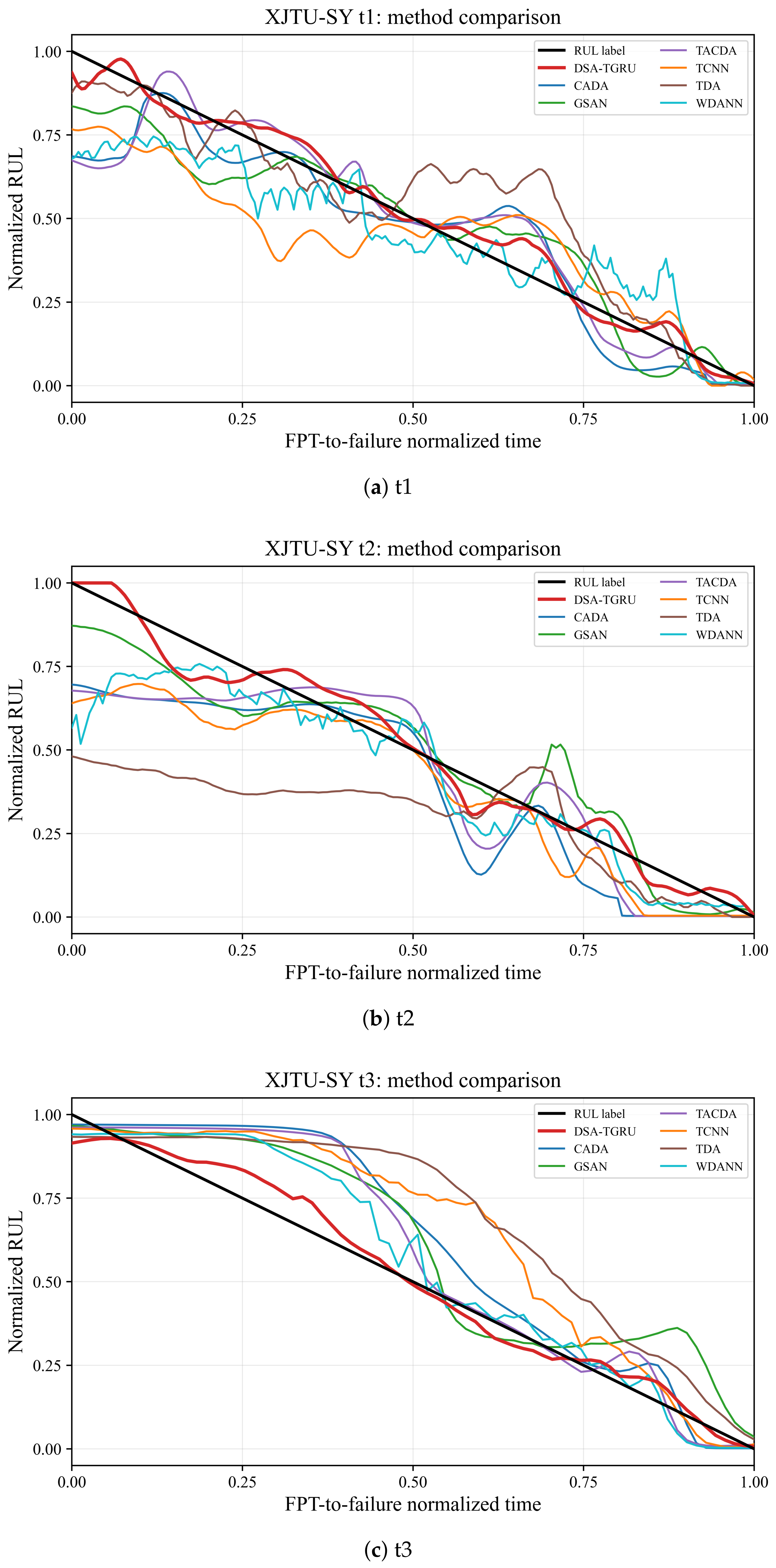
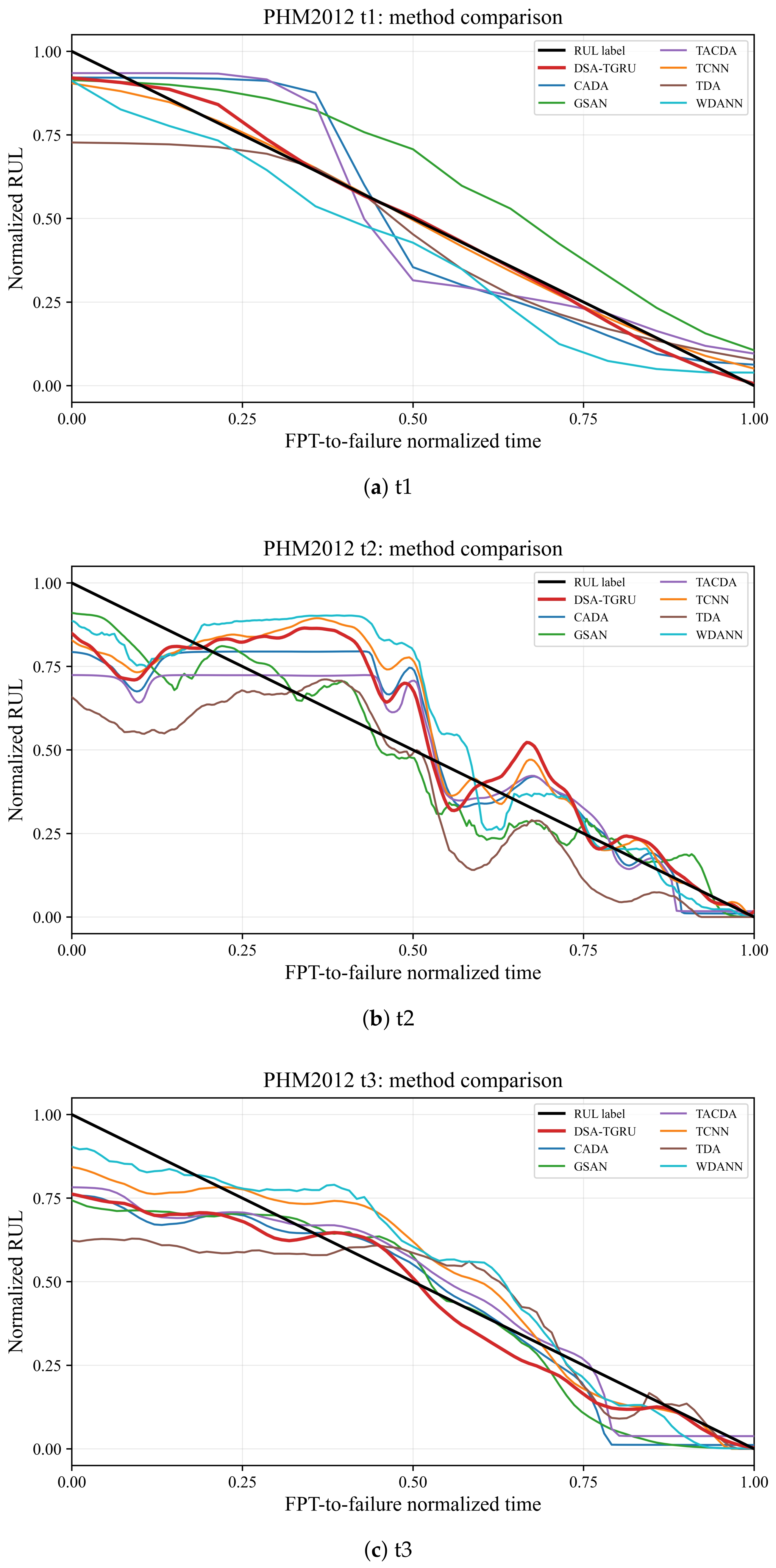
Figure 9 and Figure 10 compare the prediction curves of different methods in the t1–t3 tasks of the two datasets. Compared with most baselines, DSA-TGRU follows the true RUL trend more closely, especially on XJTU-SY.

3.7. Transfer-Contribution Control

To separate the effect of transfer learning from the effect of having labeled target-domain run-to-failure samples,

Table 12. Transfer-contribution control results (mean ± standard deviation). Source-only results are reused from the training-strategy ablation to keep a single canonical source-only baseline. Absolute errors are in post-FPT sampling segments.

Dataset	Protocol	MAE	RMSE	Abs. MAE	Abs. RMSE
XJTU-SY	Source-only	0.2866 ± 0.0949	0.3346 ± 0.1193	43.57 ± 22.84	51.07 ± 27.36
	Target-only	0.1671 ± 0.1066	0.1910 ± 0.1144	19.08 ± 4.83	22.18 ± 5.34
	S + T	0.0408 ± 0.0109	0.0521 ± 0.0152	5.99 ± 2.80	7.64 ± 3.70
	DSA-TGRU	0.0492 ± 0.0125	0.0626 ± 0.0171	7.03 ± 2.96	8.95 ± 3.97
PHM2012	Source-only	0.1368 ± 0.0540	0.1628 ± 0.0622	22.19 ± 24.41	26.22 ± 28.49
	Target-only	0.1179 ± 0.0330	0.1568 ± 0.0503	17.64 ± 16.96	23.58 ± 22.08
	S + T	0.1318 ± 0.0394	0.1543 ± 0.0441	19.81 ± 19.07	23.21 ± 22.54
	DSA-TGRU	0.0738 ± 0.0360	0.0928 ± 0.0431	12.65 ± 13.30	15.73 ± 16.31

compares four internal protocols. Source-only uses only source-domain post-FPT windows and is the same canonical result as the source-only variant in the training-strategy ablation. Target-only trains the same Transformer-GRU architecture from scratch using only target-domain post-FPT windows, without source-domain pretraining. S + T denotes source-domain pretraining followed by target-domain fine-tuning without stage-binned sampling or late-stage weighting. DSA-TGRU denotes the complete configuration.

On XJTU-SY, source-only and target-only training obtain average MAE values of 0.2866 and 0.1671, respectively, whereas S + T reduces the average MAE to 0.0408. This indicates that source-domain pretraining and target-domain fine-tuning are complementary in this dataset. However, the complete DSA-TGRU configuration has a slightly higher average MAE of 0.0492, consistent with the training-strategy ablation result that stage-binned sampling and late-stage weighting do not provide monotonic gains on XJTU-SY. On PHM2012, DSA-TGRU achieves the lowest average MAE/RMSE among the four protocols, indicating that stage-binned sampling and late-stage weighting are useful auxiliary strategies for this dataset. Therefore, the contribution of target-domain labels, source-domain pretraining, and auxiliary stage-aware training should be interpreted jointly and in a dataset-dependent manner.

3.8. Ablation Results

3.8.1. Model-Structure Ablation

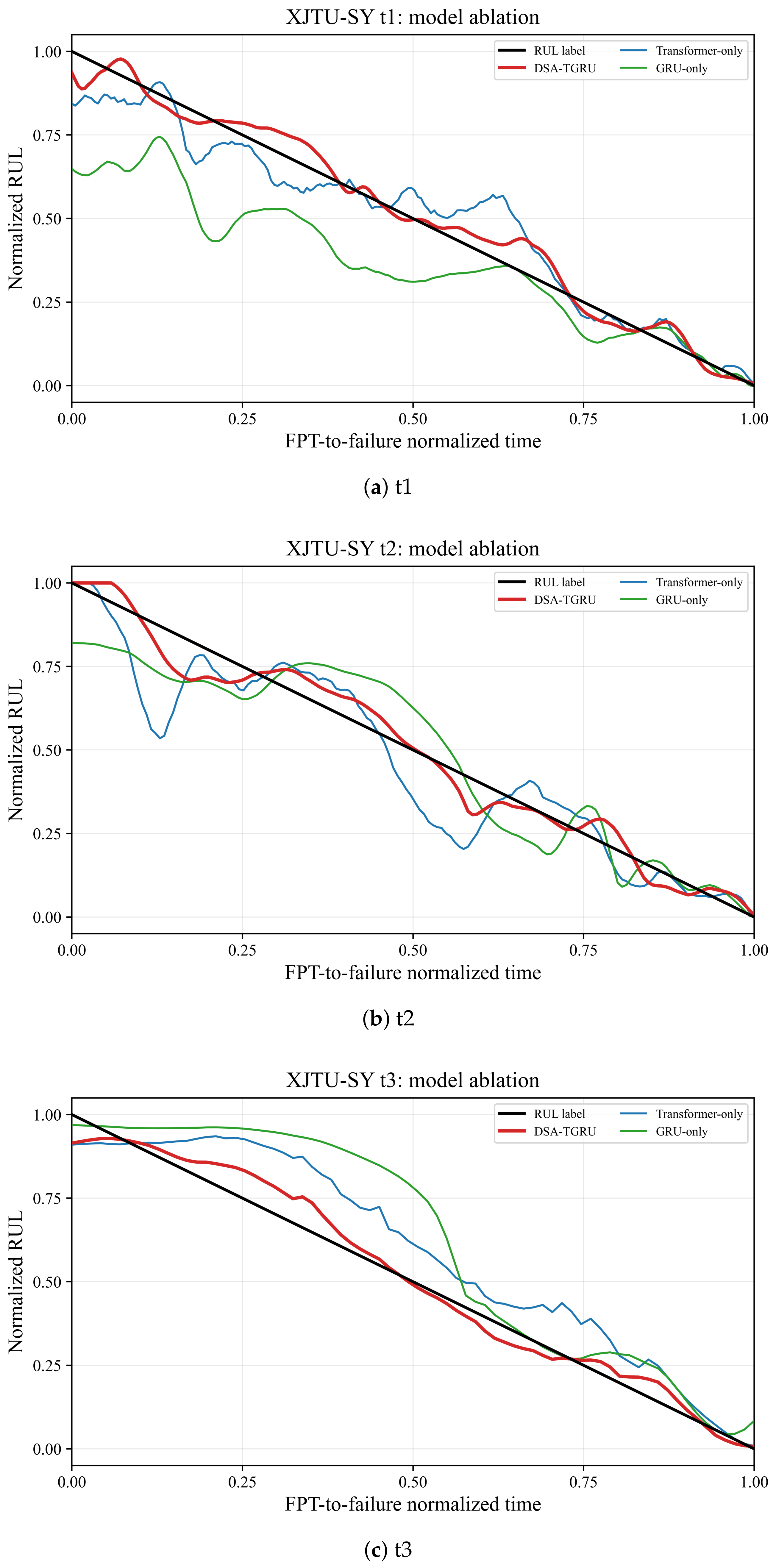
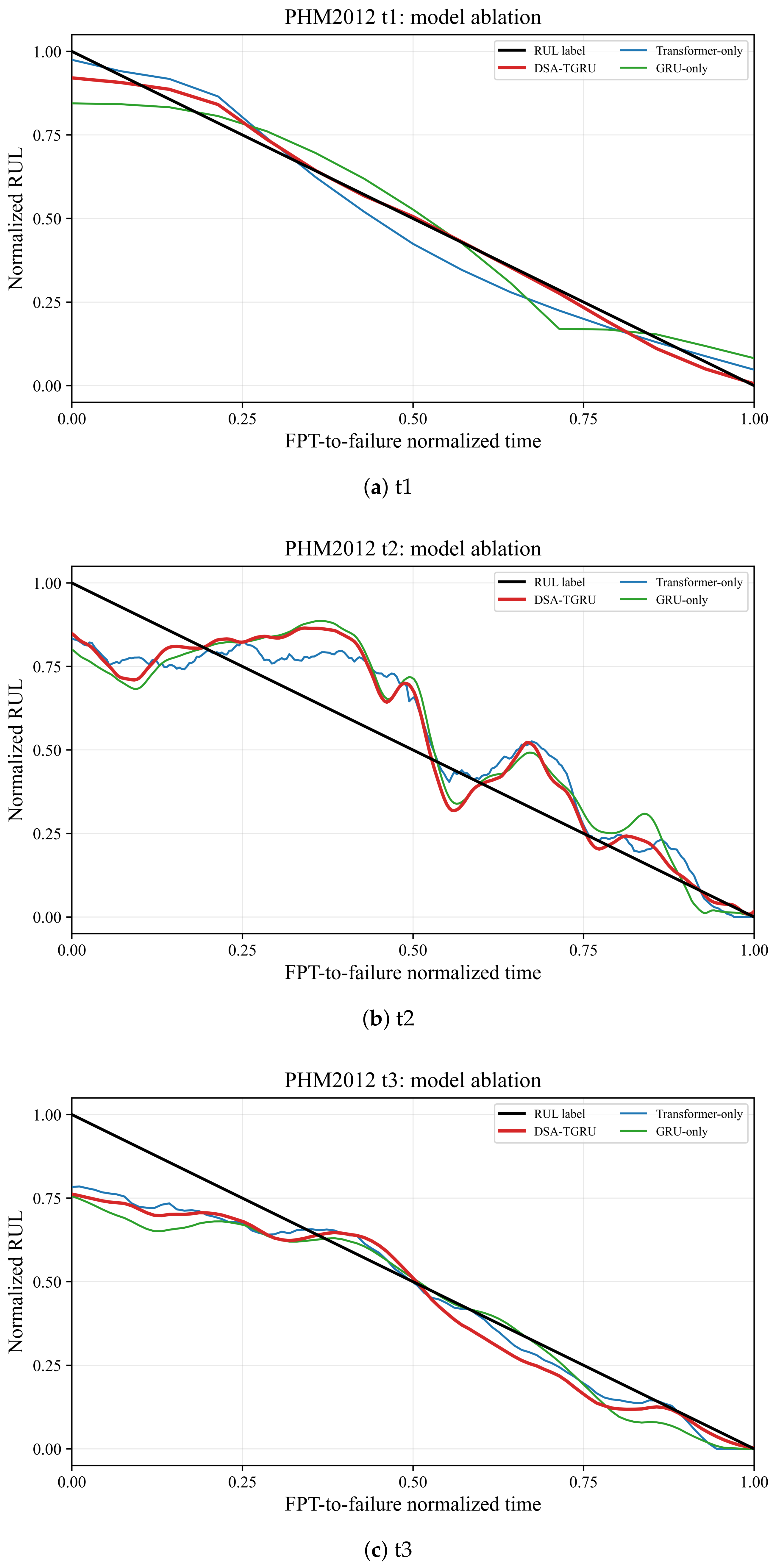
This experiment analyzes the roles of the Transformer and GRU temporal modeling modules. GRU-only removes the Transformer encoder and keeps only the GRU recurrent structure. Transformer-only removes the GRU module and keeps only the Transformer encoder and regression head. DSA-TGRU is the complete model. Figure 11 and Figure 12 show model-structure ablation prediction curves for t1–t3 tasks on the two datasets. Compared with GRU-only and Transformer-only, the complete DSA-TGRU better balances the overall decreasing trend and late-stage degradation changes.

Table 13. Model-structure ablation results (mean ± standard deviation). Absolute errors are in post-FPT sampling segments.

Dataset	Variant	MAE	RMSE	Abs. MAE	Abs. RMSE
XJTU-SY	GRU-only	0.1339 ± 0.0282	0.1670 ± 0.0407	20.03 ± 11.20	24.94 ± 14.56
	Transformer-only	0.0900 ± 0.0213	0.1116 ± 0.0231	11.99 ± 3.15	15.08 ± 4.33
	DSA-TGRU	0.0492 ± 0.0125	0.0626 ± 0.0171	7.03 ± 2.96	8.95 ± 3.97
PHM2012	GRU-only	0.0936 ± 0.0256	0.1159 ± 0.0262	14.35 ± 15.11	17.21 ± 17.31
	Transformer-only	0.0780 ± 0.0238	0.0959 ± 0.0278	12.01 ± 12.67	14.61 ± 15.03
	DSA-TGRU	0.0738 ± 0.0360	0.0928 ± 0.0431	12.65 ± 13.30	15.73 ± 16.31

reports the corresponding model-structure ablation results.

Using either GRU alone or Transformer alone degrades prediction performance. On XJTU-SY, the average MAE values of GRU-only and Transformer-only are 0.1339 and 0.0900, respectively, both higher than the 0.0492 of DSA-TGRU. On PHM2012, Transformer-only is close to the complete model and has slightly lower absolute sampling-segment errors, but DSA-TGRU still obtains the lowest normalized MAE and RMSE. This indicates that the global-dependency modeling ability of the Transformer and the recurrent temporal modeling ability of the GRU are complementary, although the structural benefit is weaker on PHM2012 than on XJTU-SY.

3.8.2. Training-Strategy Ablation

Table 14. Training-strategy ablation results (mean ± standard deviation). S, T, B, and W denote source pretraining, target fine-tuning, stage-binned sampling, and late-stage weighting, respectively. Absolute errors are in post-FPT sampling segments.

Dataset	Variant	MAE	RMSE	Abs. MAE	Abs. RMSE
XJTU-SY	Source-only	0.2866 ± 0.0949	0.3346 ± 0.1193	43.57 ± 22.84	51.07 ± 27.36
	S + T	0.0408 ± 0.0109	0.0521 ± 0.0152	5.99 ± 2.80	7.64 ± 3.70
	S + T + B	0.0496 ± 0.0116	0.0631 ± 0.0162	7.01 ± 2.80	8.91 ± 3.70
	S + T + W	0.0425 ± 0.0115	0.0546 ± 0.0156	6.21 ± 2.93	7.97 ± 3.87
	Complete method	0.0492 ± 0.0125	0.0626 ± 0.0171	7.03 ± 2.96	8.95 ± 3.97
PHM2012	Source-only	0.1368 ± 0.0540	0.1628 ± 0.0622	22.19 ± 24.41	26.22 ± 28.49
	S + T	0.1318 ± 0.0394	0.1543 ± 0.0441	19.81 ± 19.07	23.21 ± 22.54
	S + T + B	0.1274 ± 0.0334	0.1500 ± 0.0373	18.92 ± 18.61	22.21 ± 21.95
	S + T + W	0.1324 ± 0.0377	0.1552 ± 0.0417	19.56 ± 18.64	22.88 ± 21.96
	Complete method	0.0738 ± 0.0360	0.0928 ± 0.0431	12.65 ± 13.30	15.73 ± 16.31

reports progressive training-strategy ablation results. All variants use the same task splits, random seeds, and basic network, changing only target-domain fine-tuning, stage-binned sampling, and late-stage linear weighting. The source bearings, target fine-tuning bearings, checkpoint subsets, and test bearings for XJTU-SY and PHM2012 follow the t1–t3 task splits in Table 6.

Five training schemes are evaluated: source-only training, source pretraining followed by target-domain fine-tuning, target-domain fine-tuning with stage-binned sampling, target-domain fine-tuning with late-stage linear weighting, and the complete method including both stage-binned sampling and late-stage linear weighting. Source-only means that the model is trained for 300 epochs only on source-domain bearing samples without target-domain fine-tuning, stage-binned sampling, or late-stage weighting. The other variants use 200 epochs of source pretraining and 100 epochs of target-domain fine-tuning. To avoid redundant figures, this section reports ablation results only in tabular form.

Target-domain information is a key factor in reducing cross-condition errors. On XJTU-SY, the average MAE of source-only training is 0.2866, whereas adding target-domain fine-tuning reduces it to 0.0408. This shows that target-domain degradation samples can significantly correct cross-condition mapping bias. However, on this dataset, further adding stage-binned sampling or late-stage linear weighting does not form a consistent gain. The task-level decomposition in

Table 15. Task-level training-strategy ablation results. The table reports normalized MAE/RMSE for each task and separates the effects of target-domain fine-tuning (S + T), stage-binned sampling (B), and late-stage weighting (W).

Dataset	Task	Variant	MAE	RMSE
XJTU-SY	t1	S + T	0.0409 ± 0.0084	0.0534 ± 0.0128
		S + T + B	0.0458 ± 0.0085	0.0589 ± 0.0126
		S + T + W	0.0433 ± 0.0092	0.0563 ± 0.0140
		Complete method	0.0466 ± 0.0085	0.0610 ± 0.0138
	t2	S + T	0.0432 ± 0.0044	0.0532 ± 0.0058
		S + T + B	0.0494 ± 0.0071	0.0616 ± 0.0104
		S + T + W	0.0431 ± 0.0050	0.0539 ± 0.0067
		Complete method	0.0494 ± 0.0082	0.0608 ± 0.0102
	t3	S + T	0.0382 ± 0.0177	0.0496 ± 0.0245
		S + T + B	0.0535 ± 0.0176	0.0687 ± 0.0241
		S + T + W	0.0410 ± 0.0188	0.0535 ± 0.0246
		Complete method	0.0516 ± 0.0197	0.0662 ± 0.0266
PHM2012	t1	S + T	0.0833 ± 0.0249	0.1004 ± 0.0265
		S + T + B	0.0914 ± 0.0250	0.1102 ± 0.0263
		S + T + W	0.0876 ± 0.0305	0.1062 ± 0.0336
		Complete method	0.0294 ± 0.0093	0.0388 ± 0.0092
	t2	S + T	0.1641 ± 0.0096	0.1935 ± 0.0107
		S + T + B	0.1594 ± 0.0074	0.1878 ± 0.0083
		S + T + W	0.1609 ± 0.0094	0.1893 ± 0.0106
		Complete method	0.1104 ± 0.0143	0.1365 ± 0.0131
	t3	S + T	0.1481 ± 0.0121	0.1691 ± 0.0124
		S + T + B	0.1316 ± 0.0177	0.1519 ± 0.0178
		S + T + W	0.1486 ± 0.0102	0.1700 ± 0.0101
		Complete method	0.0814 ± 0.0068	0.1031 ± 0.0084

shows the same pattern: S + T has the lowest MAE/RMSE on XJTU-SY t1, t2, and t3. The complete method has an average MAE of 0.0492, higher than the target-fine-tuning-only variant. Therefore, XJTU-SY ablation results indicate that target-domain fine-tuning contributes most clearly, while the benefits of stage-binned sampling and late-stage weighting are task-dependent. On PHM2012, the complete method achieves an average MAE of 0.0738 and an average RMSE of 0.0928, lower than source-only training and all single-substrategy variants, and it also has lower errors than the single-substrategy variants on all three tasks in Table 15. This indicates that stage-binned sampling and late-stage weighting provide auxiliary benefits on PHM2012, but this conclusion should not be generalized as a monotonic benefit on all datasets.

3.8.3. HI Input Comparison

To examine whether PCA-HI should be used as a prediction-model input, three input forms are compared: only the nine selected features, only the one-dimensional HI, and the nine features concatenated with HI to form a 10-dimensional input. The HI input comparison uses the same t1–t3 task splits, random seeds, and basic network as the training-strategy ablation. All three input forms use the same source pretraining, target-domain fine-tuning, stage-binned sampling, and late-stage linear weighting strategy. The results are shown in

Table 16. HI input comparison results (mean ± standard deviation). Absolute errors are in post-FPT sampling segments.

Dataset	Input	MAE	RMSE	Abs. MAE	Abs. RMSE
XJTU-SY	Nine features	0.0492 ± 0.0125	0.0626 ± 0.0171	7.03 ± 2.96	8.95 ± 3.97
	HI-only	0.1481 ± 0.0400	0.1813 ± 0.0376	19.61 ± 4.87	24.63 ± 7.26
	Nine features + HI	0.0472 ± 0.0063	0.0609 ± 0.0090	6.75 ± 2.62	8.69 ± 3.47
PHM2012	Nine features	0.0738 ± 0.0360	0.0928 ± 0.0431	12.65 ± 13.30	15.73 ± 16.31
	HI-only	0.0977 ± 0.0418	0.1171 ± 0.0483	16.30 ± 18.97	19.50 ± 22.40
	Nine features + HI	0.1334 ± 0.0349	0.1559 ± 0.0406	19.37 ± 18.35	22.65 ± 21.63

. This experiment is also presented only in tabular form.

The response to HI input is inconsistent across datasets. On XJTU-SY, HI-only is much weaker than multidimensional feature input, indicating that a single HI loses local impact statistics, spectral shape, and time-frequency energy information. Nine features + HI slightly improves over nine features, but the improvement is small. On PHM2012, the main nine-feature input still obtains the lowest average error, and neither HI-only nor nine features + HI outperforms the main result. This indicates that directly using PCA-HI as a prediction input does not necessarily produce consistent gains. More importantly, PCA-HI depends on offline full-life trajectories for normalization and degradation-process retrospection. If it is used as a main prediction input, the model would further depend on complete offline trajectories. Therefore, the main model uses the nine selected features as inputs, and PCA-HI is mainly used for FPT identification, label construction, and degradation-process interpretation.

3.9. Stability and Significance Analysis

To evaluate stability across random seeds, standard deviations of main tasks are reported, and a two-sided Wilcoxon signed-rank test is used to compare DSA-TGRU with baselines and ablation variants. The sample unit of the test is paired MAE/RMSE at the task-by-random-seed level. Each dataset contains three tasks and five random seeds, giving $n=15$ paired samples. Window-level errors are not used as significance-test samples, avoiding artificial sample-size inflation. No multiple-comparison correction is applied; the significance results are used mainly as robustness evidence. In the main results, the MAE standard deviations of the three XJTU-SY tasks are 0.0085, 0.0082, and 0.0197, respectively. The corresponding PHM2012 values are 0.0093, 0.0143, and 0.0068. Except for XJTU-SY task t3 and PHM2012 task t2, which show relatively larger fluctuations, the other tasks maintain stable error levels across random seeds.

The significance results are listed in

Table 17. Wilcoxon signed-rank test results. S, T, B, and W denote source pretraining, target fine-tuning, stage-binned sampling, and late-stage weighting. “DSA” and “Comp.” denote DSA-TGRU and the comparison object, respectively; n.s. denotes not significant.

Dataset	Group	Comparison	MAE p	RMSE p	Result
XJTU-SY	Baseline	CADA	$6.10\times {10}^{-5}$	$6.10\times {10}^{-5}$	DSA better
		GSAN	$6.10\times {10}^{-5}$	$6.10\times {10}^{-5}$	DSA better
		TACDA	$6.10\times {10}^{-5}$	$6.10\times {10}^{-5}$	DSA better
		TCNN	$6.10\times {10}^{-5}$	$6.10\times {10}^{-5}$	DSA better
		TDA	$6.10\times {10}^{-5}$	$6.10\times {10}^{-5}$	DSA better
		WDANN	$6.10\times {10}^{-5}$	$6.10\times {10}^{-5}$	DSA better
	Structure	GRU-only	$6.10\times {10}^{-5}$	$6.10\times {10}^{-5}$	DSA better
		Transformer-only	$6.10\times {10}^{-5}$	$1.22\times {10}^{-4}$	DSA better
	Training	Source-only	$6.10\times {10}^{-5}$	$6.10\times {10}^{-5}$	DSA better
		S + T	$6.10\times {10}^{-5}$	$6.10\times {10}^{-5}$	Comp. better
		S + T + B	1.0000	0.6387	n.s.
		S + T + W	$1.83\times {10}^{-4}$	$1.22\times {10}^{-4}$	Comp. better
	HI input	HI-only	$6.10\times {10}^{-5}$	$6.10\times {10}^{-5}$	DSA better
		9 features + HI	0.4212	0.5995	n.s.
PHM2012	Baseline	CADA	0.0353	0.0151	DSA better
		GSAN	0.0730	0.0833	n.s.
		TACDA	0.0833	0.0637	n.s.
		TCNN	0.0054	0.0125	DSA better
		TDA	$6.10\times {10}^{-5}$	$6.10\times {10}^{-5}$	DSA better
		WDANN	0.0026	0.0043	DSA better
	Structure	GRU-only	0.0054	0.0012	DSA better
		Transformer-only	0.5245	0.7615	n.s.
	Training	Source-only	$1.22\times {10}^{-4}$	$1.22\times {10}^{-4}$	DSA better
		S + T	$6.10\times {10}^{-5}$	$6.10\times {10}^{-5}$	DSA better
		S + T + B	$6.10\times {10}^{-5}$	$6.10\times {10}^{-5}$	DSA better
		S + T + W	$6.10\times {10}^{-5}$	$6.10\times {10}^{-5}$	DSA better
	HI input	HI-only	0.0125	0.0103	DSA better
		9 features + HI	$6.10\times {10}^{-5}$	$6.10\times {10}^{-5}$	DSA better

. On XJTU-SY, DSA-TGRU is significantly better than all baselines, model-structure ablation variants, and source-only training. However, compared with “source pretraining + target fine-tuning” and “source pretraining + target fine-tuning + late-stage linear weighting”, DSA-TGRU has higher errors, consistent with the observation in Table 14 that stage-aware substrategies do not bring monotonic gains on XJTU-SY. The PHM2012 results are more complex: DSA-TGRU reaches significance against CADA, TCNN, TDA, WDANN, and GRU-only in normalized MAE/RMSE, but not against GSAN, TACDA, or Transformer-only at the 0.05 level. This is consistent with the small differences among methods and the larger t2 fluctuation in PHM2012. The Wilcoxon tests for the progressive training-strategy and HI input comparisons also use task-by-random-seed paired samples, with the main DSA-TGRU result as the baseline.

4. Discussion

The stronger advantage of DSA-TGRU on XJTU-SY is mainly due to clearer degradation representation in this dataset. The nine selected features of XJTU-SY show more distinct amplitude enhancement and impact changes before failure, and the PCA-HI has higher trendability and late-stage increase. The post-FPT segments identified by ATMROC cover the true degradation stage more effectively, so the proportion of training samples directly related to failure development is higher. In this case, degradation-start constraints and target-domain fine-tuning reduce the interference caused by stationary healthy-stage segments and cross-condition distribution differences, allowing Transformer-GRU to learn target-condition degradation patterns more easily. However, the progressive ablation also shows that stage-binned sampling and late-stage linear weighting do not further reduce average errors beyond target-domain fine-tuning alone on XJTU-SY. This indicates that the benefits of stage-aware substrategies depend on dataset degradation morphology and target-domain sample composition.

PHM2012 task t2 is more difficult mainly because degradation occurs later and cross-condition differences are more pronounced. In PHM2012, most bearings show obvious degradation only near the end of life, and average HI trendability and late-stage increase are lower than those of XJTU-SY. For task t2, the test bearing Bearing1_4 has a relatively late FPT, fewer post-FPT training and evaluation windows, and stronger differences in degradation speed and signal fluctuation between source C2 bearings and target C1 bearings. In this situation, the target-domain fine-tuning stage has limited usable degradation information, and the model is more likely to deviate in the rapid late-stage decline region. Therefore, although DSA-TGRU maintains the best average normalized MAE/RMSE on PHM2012, it is not always superior to all methods in task t2 or in absolute sampling-segment errors.

The necessity of target-domain fine-tuning lies in correcting cross-condition feature–RUL mappings. Source-only training can learn general temporal degradation patterns, but differences in load, rotational speed, noise level, and degradation rate across operating conditions change the mapping between features and RUL labels. The target-only control further shows that target-domain labels alone are informative, but they do not fully replace transfer learning. On XJTU-SY, target-only training is clearly better than source-only training but remains much worse than S + T, indicating that source-domain pretraining and target-domain fine-tuning provide complementary information. On PHM2012, the complete method is better than source-only, target-only, and S + T, suggesting that late-stage sampling and weighting help when degradation occurs late and the post-FPT data are limited. Thus, under the offline engineering protocol studied here, introducing target-domain information is important, but the best configuration should be selected according to dataset degradation morphology and target-domain sample composition.

The main model uses the nine features rather than directly using HI, mainly to preserve multidimensional local degradation information and to avoid further dependence on complete offline trajectories. The HI input comparison shows that HI-only is much weaker than multidimensional features on XJTU-SY, indicating that one-dimensional HI compression loses local degradation information. On XJTU-SY, the error of nine features + HI is slightly lower than that of the nine-feature input, but the Wilcoxon test does not reach significance. On PHM2012, neither HI-only nor nine features + HI outperforms the main nine-feature result. Considering that HI in this paper depends on offline full-life retrospective analysis, using it as a main model input would increase the dependence of prediction on complete offline trajectories. Therefore, this paper treats HI as a tool for FPT identification and label construction rather than as a universal prediction input feature.

The source-domain normalization control highlights another important boundary of the present protocol. Full-life normalization is not a label input and does not use the test bearing for parameter updating or checkpoint selection, but it may introduce future scale information through the global feature range. The control experiment shows that prediction errors increase under source-domain Min–Max normalization, especially on XJTU-SY. This should be interpreted as sensitivity to the normalization protocol rather than direct proof that the full-life results depend on information leakage, because source-domain scaling also creates a difficult cross-condition range-coverage problem. Nevertheless, the result confirms that the main full-life normalization results should be treated as offline retrospective results rather than online prediction performance.

The proposed method still has limitations. First, the feature-selection scheme uses a fixed candidate feature set and fixed removal of an unstable feature. Although this improves interpretability and protocol consistency, its adaptability to different equipment, fault types, and sampling conditions remains limited. Second, ATMROC degradation-start identification depends on the trend quality of PCA-HI. When the HI variation is weak or abrupt degradation occurs very late, the identified FPT may be delayed, reducing the number of available degradation-stage training samples. Third, this paper uses a linear RUL label after FPT, whereas real bearing degradation may show nonlinear, stage-wise, or sudden failure behavior. Fourth, the full-life normalization and PCA-HI construction steps are offline retrospective operations and are not directly applicable to online deployment with incomplete degradation trajectories. Fifth, because of the limited number of available run-to-failure bearings, the checkpoint metric is computed on data drawn from target fine-tuning bearings rather than from a fully independent target bearing. Although the test bearing is still excluded from parameter updating and model selection, checkpoint selection on a non-independent target bearing may introduce optimistic bias, especially in PHM2012 where the number of available target bearings is small. Finally, the experimental setting is offline target-domain fine-tuning with a small number of labeled samples and does not cover fully unlabeled target domains, online incremental updating, or real-time early prediction. Further evaluation under stricter normalization protocols, independent checkpoint-selection bearings, and more industrial devices is required.

5. Conclusions

This paper proposes a degradation-stage-aware Transformer-GRU method for cross-condition bearing RUL prediction under an offline full-life retrospective analysis protocol. The method addresses healthy-stage sample interference, limited labeled target-domain degradation samples, and degradation-pattern differences. It first extracts time-domain, frequency-domain, and time-frequency-domain features from raw vibration signals and constructs nine input features using fixed degradation-sensitive feature selection. Then, PCA-HI and ATMROC are used to identify the bearing degradation start, and RUL labels are constructed only from post-FPT samples. Finally, a Transformer-GRU hybrid network performs temporal modeling, and cross-condition prediction is conducted through source-domain pretraining and fine-tuning with a small number of labeled target-domain samples. Stage-binned sampling and late-stage weighting are analyzed as auxiliary training substrategies.

Experiments on the XJTU-SY and PHM2012 datasets show that DSA-TGRU obtains average normalized MAE values of 0.0492 and 0.0738 and average normalized RMSE values of 0.0626 and 0.0928, respectively. In normalized MAE and RMSE, it generally outperforms CADA, GSAN, TACDA, TCNN, TDA, and WDANN. In absolute sampling-segment errors, the proposed method has a clear advantage on XJTU-SY and is close to some methods on PHM2012.

Ablation experiments further show that the Transformer-GRU hybrid structure outperforms single temporal modeling modules in normalized errors and that target-domain fine-tuning after source-domain pretraining is an important factor in reducing cross-condition prediction errors. The target-only control confirms that target-domain labels themselves contribute substantially, while the comparison among source-only, target-only, S + T, and DSA-TGRU indicates that the value of source pretraining and auxiliary stage-aware training differs across datasets. Stage-binned sampling and late-stage linear weighting provide auxiliary benefits on PHM2012, but they do not form monotonic gains over target-domain fine-tuning alone on XJTU-SY. Their effectiveness is therefore dataset- and task-dependent. The source-domain normalization control further shows that the results are sensitive to the normalization protocol; consequently, the main results should be understood as offline full-life retrospective results rather than online prediction performance. The HI input comparison shows that HI-only and nine features + HI do not consistently outperform the main nine-feature input, so PCA-HI is mainly used for FPT identification and label construction. Significance analysis further supports the advantage of the proposed method in most normalized-error comparisons, while also showing that the differences against some training-strategy variants on XJTU-SY and against GSAN, TACDA, and Transformer-only on PHM2012 are not significant.

In summary, the main contribution of this paper is to embed degradation-start identification explicitly into RUL sample construction, reducing the interference of stationary healthy-stage samples. The paper also builds a temporal prediction model combining Transformer and GRU to use both global dependencies and local recurrent information. In addition, it verifies the key role of source-domain pretraining and target-domain fine-tuning under the offline cross-condition protocol and clarifies that stage-binned sampling and late-stage linear weighting are auxiliary strategies with dataset-dependent benefits. Future work will investigate online normalization without test-trajectory participation, adaptive feature selection, nonlinear RUL label construction, uncertainty estimation, and online incremental updating, and will evaluate the method on more industrial equipment and practical operating conditions.