In this paper, we propose a gradient estimation method for quantization of neural network models. First, we present a novel approach to approximate the non-differentiable rounding function in the quantization process, ensuring its differentiability over all values. Building on this, our method enables effective optimization of quantization parameters, model weights and bit-widths, either independently or jointly, to improve overall quantization accuracy.
3.1. Gradient Estimation
In this section, we first discuss the origin of quantization errors, which arise from the discrepancy between the original values and their quantized counterparts. Based on this understanding, we then construct an approximate quantization function that is differentiable at all points.
We begin by introducing the sources of quantization error. For quantization in neural networks [
19], the weights and activations of each layer are quantized. In detail, this is accomplished by taking two steps for each layer: one for the weights and one for the activations. For each layer, we first determine the clipping thresholds [
,
] according to the value range, and then clip the weights to this interval.
Considering weight quantization, where the weight is represented by
, the quantization formula is as follows:
where
s is the scaling factor that maps floating-point value
into the integer space, and
D is the zero-point, the value
D that the real value zero is mapped to. The scaling factor
s is a quantization parameter that influences the precision of quantization.
A clamp operation is applied after the rounding operator, which is defined as:
To simulate the numerical error introduced by quantization, a quantization and dequantization operation is applied to the weight and activation of each layer. The complete quantization operation for weights is defined as follows:
where
is the floating-point value of the weight after quantization and dequantization, capturing the quantization error. For activation values, the quantization method is similar.
It should be noted that Equations (1)–(3) describe a conventional quantization and dequantization formulation, in which clipping and rounding are commonly used. These equations are introduced to illustrate the source of non-smooth operations in standard quantization. The proposed method in this work is the differentiable surrogate rounding function a(x) defined in Equation (
6). Therefore, the “everywhere differentiable” property claimed in this paper refers specifically to the proposed surrogate a(x), whose derivative is given in Equation (
7), rather than to the conventional quantization formulation in Equations (1)–(3).
Building on our discussion of quantization error sources, we address the issue of non-differentiability in the quantization process by introducing a method to construct a differentiable approximation of the quantization function. In quantization, the error between the actual values and the quantized values primarily originates from the rounding function,
r(
x) =
round(
x). Therefore, the difference between the rounded values and the original values can be expressed as:
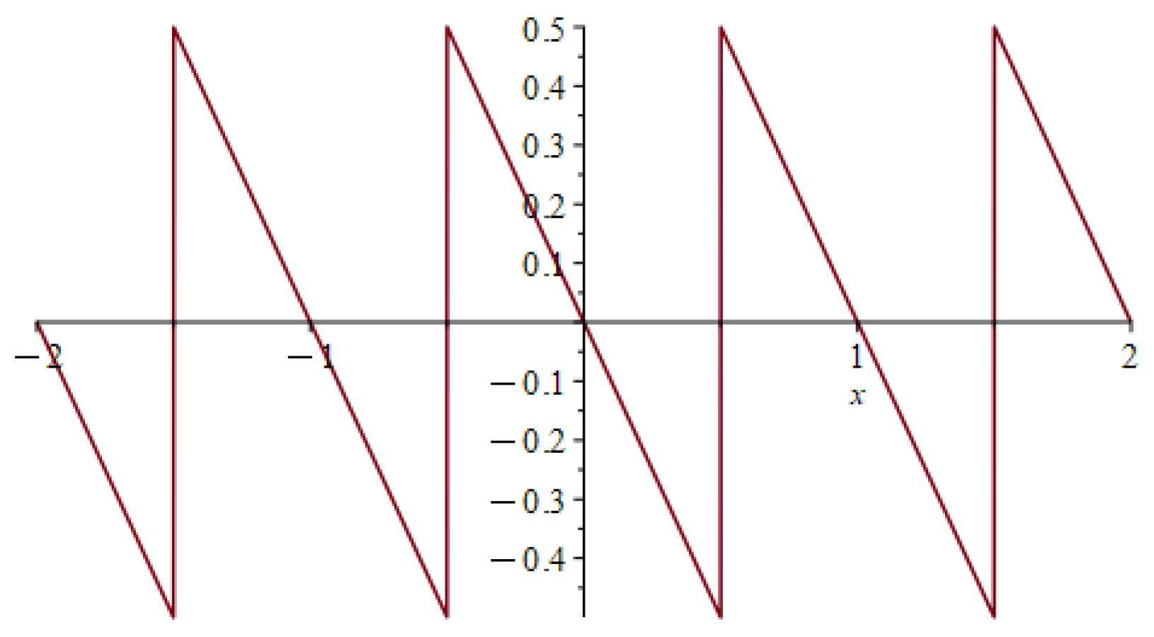
is illustrated in
Figure 1.
Figure 1 shows that that the difference between the rounding function and the original linear function is a sawtooth wave function swt(x) with a period of 1 and an amplitude of 1.
To approximate the sawtooth wave function, we employ a novel combination of the arccos, arctan, and sine functions. Although these functions are not typically used for generating standard sawtooth or square waves, their specific combinations and transformations allow us to create a function that mimics the desired waveform. This design achieves a close approximation to the target sawtooth wave, essential for maintaining differentiability in the quantization process. The mathematical formulation of the designed sawtooth wave function
is as follows:
The intuition behind this function’s design is to transform a standard periodic wave into the desired sawtooth shape. Specifically, the term provides the fundamental periodic waveform. The arccos and arctan functions then act as a composite shaping operator, which stretches and sharpens the smooth sine curve to precisely mimic the linear segments and abrupt turning points of a true sawtooth wave.
This function
represents the error between the rounding operation and the identity function; by adding it back to the linear function
, we obtain the final differentiable approximation
for the rounding function
:
In the above equation,
f is an approximate parameter that controls the smoothness of the curve. The approximate function
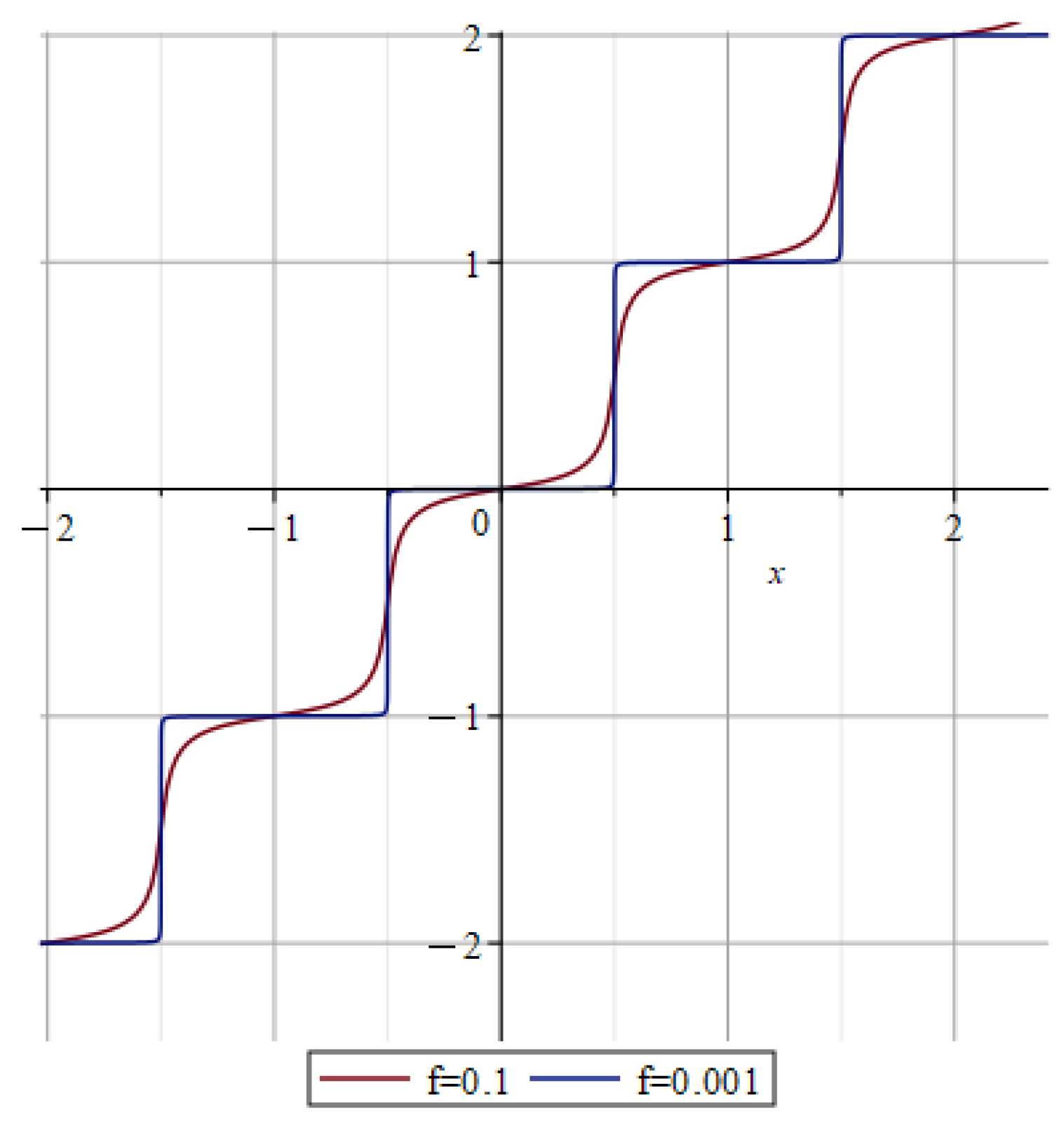
is shown in the
Figure 2, with red line being
f = 0.1 and blue line being
f = 0.001.
With respect to approximation properties and optimization stability, the proposed rounding surrogate uniformly approximates : there exists a function as such that ;
Figure 2 shows that the smaller
f is, the steeper the approximate rounding operator
and the closer it is to the original rounding operator
. When
f is sufficiently small (e.g.,
),
becomes visually indistinguishable from
at plot scale; formally, the uniform gap is bounded by
. Here
denotes a uniform error bound that depends only on the smoothness
f and satisfies
as
. By controlling the parameter
f, the differentiability of the backpropagation calculation process can be placed in a suitable numerical range. While making the model easy to converge, it effectively improves the calculation accuracy of the model and reduces the accuracy loss caused by quantization. These properties explain why decreasing
f tightens the approximation while preserving well-behaved gradients, enabling stable end-to-end training.
Given the bounded-derivative property above, we adopt
as a stable surrogate of
during backpropagation. Then, the gradient of
is used to approximate the gradient of the rounding operator
, as follows:
To further clarify the role of the smoothness parameter
f, we analyze its effect from two perspectives: approximation accuracy and gradient magnitude. Since the true rounding function is discontinuous at half-integer points, the maximum pointwise error is dominated by the discontinuity region. Therefore, we use the mean approximation error to characterize the overall approximation fidelity. For a given normalized input range
, the empirical mean approximation error is defined as:
where
denotes the proposed surrogate under a specific value of
f, and
denotes the sampled normalized input values.
measures the average deviation between the proposed surrogate and the true rounding function within the considered normalized input range.
To characterize the gradient behavior, we further define the maximum surrogate gradient magnitude as:
According to Equation (
7), decreasing
f makes the transition regions sharper and increases the peak gradient magnitude near half-integer points. Therefore,
f controls a trade-off between approximation fidelity and gradient magnitude.
Table 2 reports
and
under different values of
f. As shown in
Table 2, smaller
f values lead to lower mean approximation error
, and they also produce larger maximum gradient magnitudes
. This result indicates that
f should not be selected solely to minimize the approximation error. Instead, it should be chosen to balance the closeness to the rounding function and the smoothness of the surrogate gradients during optimization.
Therefore, the gradient of the pseudo-quantization operator with the proposed approximate rounding operator
with respect to the input can be expressed as Equation (10).
In which, the formula for
is as follows:
In order to solve the problem that the rounding function is nondifferentiable, this paper creatively proposes a gradient approximation method to approximate the rounding function. It captures the sawtooth’s period, amplitude, and crucial sharp transitions, more effectively than generic smoothers. It enables the proposed approximate rounding operator to automatically compute gradients in the backpropagation process of quantization-aware training. In this way, the weight, quantization bit-width, and quantization parameters can be optimized independently or cooperatively, and the accuracy loss caused by quantization can be further reduced.
3.2. Quantization Parameter Optimization
Traditional quantization-aware training updates only weights and quantization parameters, calculating the quantization parameters post-weight iteration based on layer activations and weights. This decoupled update mechanism between quantization parameters and weights may lead to suboptimal results. In contrast, our proposed method enables both separate and joint optimization of weights, bitwidths, and quantization parameters, allowing more direct learning of optimal quantization configurations. This paper focuses specifically on the co-optimization mechanism between neural network model weights and quantization parameters. Other optimization methods follow fundamentally similar principles and thus will not be further discussed.
During training, pseudo-quantization is applied to both inputs and weights of each convolutional and fully connected layer. These operations estimate the data distribution and compute quantization parameters during network training. They simulate the quantization procedure and its induced error, and compensate for such errors via iterative training. For quantization-parameter calibration, we use an MSE reconstruction loss between the high-precision layer outputs and the corresponding quantized outputs. For task-level QAT/fine-tuning, the original task loss is retained. In the backpropagation phase, parameter updates are computed analytically via derivatives, instead of heuristically estimating the range of activations and weights. Pseudo-quantization yields a more uniform distribution of weights and activations, resulting in smaller accuracy degradation compared with direct post-quantization. Furthermore, constraining each layer’s output within a reasonable range effectively avoids overflow issues. Integrating quantization into network training enables reasonable weight discretization, reduces rounding-induced accuracy loss, and further improves the overall performance of quantized neural networks.
In this method, the optimization model is solved based on the generated initial quantization parameters, and the differentiable quantization parameters are automatically optimized.
3.3. Bit-Width Allocation Using Inter-Layer Sensitivity Analysis
Models with mixed bit-widths often lead to a significant decrease in model accuracy while reducing model computational complexity and improving computational efficiency. How to allocate bit widths more effectively while preserving accuracy remains an important problem. Sensitive layers and non-sensitive layers are defined based on the magnitude of accuracy loss before and after quantization. Layers with a larger decrease in accuracy are considered sensitive layers. The current basic bit-width allocation strategy is to assign higher bit-widths to sensitive layers and lower bit-widths to non-sensitive layers. Based on the hyperparameter
f in the approximate round function, we propose a method for inter-layer sensitivity analysis [
20].
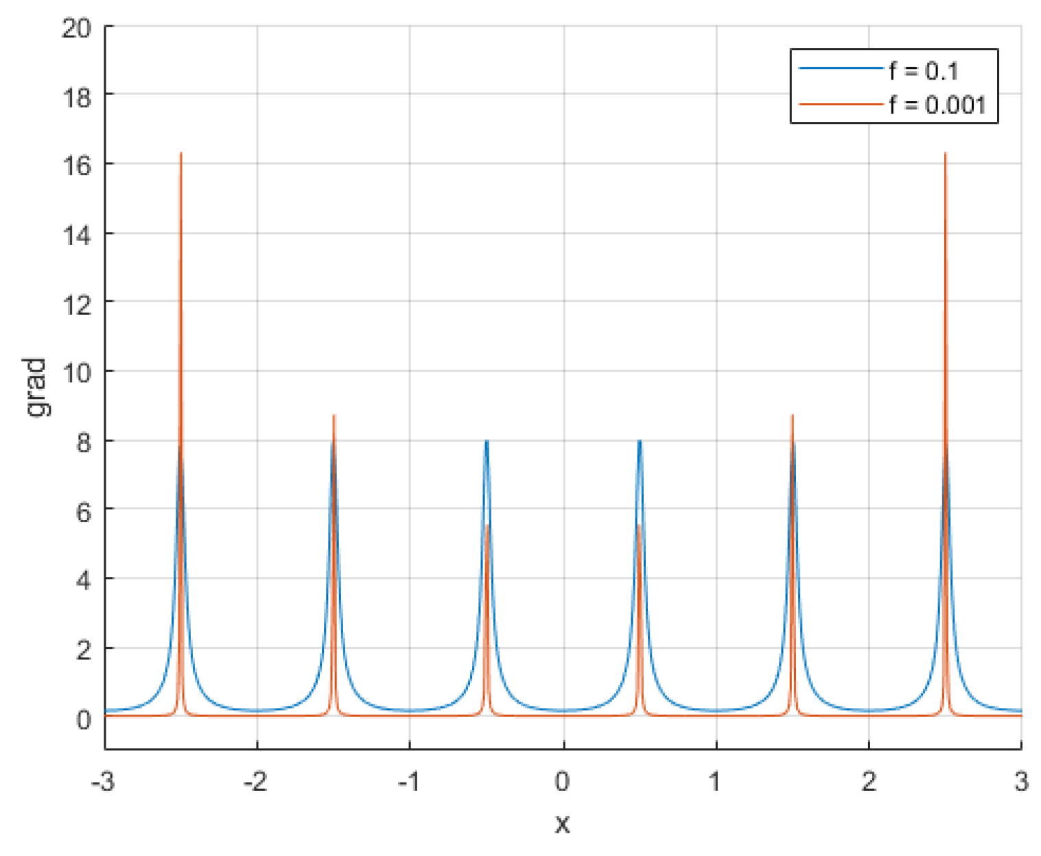
As shown in
Figure 3, it can be seen that the smaller the value of
f, the sharper the derivative of the approximate round function will be. In backpropagation training, the smaller the
f value of the approximate round function, the larger the calculated gradient, which leads to a larger step size for parameter updates. For sensitive layers, a larger step size often results in a significant decrease in accuracy. Therefore, we optimize the
f parameter individually through fine-tuning, guiding the changes in
f parameters across different layers. For sensitive layers, only by increasing the
f value can we ensure an improvement in training accuracy. Non-sensitive layers exhibit much smaller parameter changes compared to sensitive layers due to their insensitivity to layer alterations.
By adaptively learning a separate
f for each layer during training, we obtain layer-wise
f values after fine-tuning. These learned values indicate the quantization sensitivity of different layers. Based on this observation, we assign lower bit-widths to less sensitive layers, thereby reducing the BOPS [
21] of the mixed-precision model relative to a standard 8-bit configuration. First, we fix the quantization parameters and network weights to optimize the layer-wise
f values and obtain the quantization sensitivity of each layer. Layers with lower sensitivity are assigned lower bit-widths. Subsequently, with the bit-widths and
f values fixed, we jointly optimize the weights and quantization parameters to drive the model toward optimal convergence. In this way, our framework supports both independent and joint co-optimization of weights, bit-widths, and quantization parameters.
It should be noted that the proposed f-based sensitivity indicator is not intended to replace all existing sensitivity metrics from a theoretical perspective. Instead, it provides a lightweight, gradient-aware sensitivity measure that is naturally integrated with the proposed differentiable rounding surrogate. Compared with Hessian-based sensitivity metrics, which usually require second-order information or additional approximation, the proposed indicator can be obtained during the optimization of the surrogate parameter f. Therefore, it offers a practical alternative for guiding mixed-precision allocation within the proposed differentiable quantization framework.
Extremely low-bit settings such as W1A1 suffer from unavoidable severe accuracy loss, making them difficult for practical deployment and large-scale application. Therefore, this work mainly focuses on practical 4-bit quantization configurations, which can achieve a good balance between inference performance and compression efficiency. We leave the adaptive automatic scheduling of layer-wise f under various ultra-low-bit scenarios as a valuable direction for future research.