UAV Three-Dimensional Path Planning Based on Improved Dung Beetle Optimizer Algorithm

Abstract

The rapid advancement of unmanned aerial vehicles (UAVs) has greatly increased the application of various swarm intelligence algorithms in UAV path planning. To address the potential issues with the dung beetle optimizer (DBO) in UAV trajectory planning, such as low convergence accuracy, tendency to get trapped in local optima, and imbalance between global search and local exploration, a hybrid algorithm termed DBO-PSO is proposed by integrating DBO with particle swarm optimization (PSO) to solve the UAV path planning model. The Kent chaotic map is introduced to enhance population diversity and distribution uniformity, and the velocity–position update mechanism of PSO is incorporated into DBO to strengthen its global search capability. Comparative experiments are conducted on CEC2022 benchmark functions, and multiple classical swarm intelligence algorithms are selected for comparison using six evaluation metrics, along with Wilcoxon rank-sum and Friedman statistical tests. An ablation study is also performed to evaluate the contribution of each improvement component. The path planning experimental results demonstrate that compared to DBO, PSO, IDBO, and ECFDBO under the population size of 50, DBO-PSO reduces the total path cost by 44.2%, 17.3%, 8.9%, and 45.1%, respectively. The ablation study verifies that both improvement components contribute positively, which demonstrates its competitive performance and practical applicability in UAV three-dimensional path planning. The source codes to support the presented results are publicly available on GitHub.

1. Introduction

In recent years, benefiting from the rapid advancement of the social economy and technology, unmanned aerial vehicles (UAVs) have been recognized as a potential solution in many aspects due to their outstanding advantages such as their flexibility, low cost, high efficiency and versatility. They have been widely used and have demonstrated extensive successful applications in various fields such as smart logistics [1], disaster search and rescue [2], agricultural irrigation [3] and others [4,5]. The reasonable arrangement of UAVs is considered essential for the efficient execution of smart logistics tasks, in which path planning technology is regarded as a critical component. Under various constraints including flight safety, energy consumption, and obstacle avoidance, a path planning problem is always rendered as a typical complex high-dimensional, constrained optimization problem.

Path planning algorithms have undergone significant development during the past few years. Currently, they can mainly be categorized into three major classes: traditional, metaheuristic and deep reinforcement learning (DRL-based). Traditional algorithms include typical representatives such as artificial potential field (APF) [6], linear programming [7], A* [8], D* [9], rapid random tree (RRT) [10,11], etc., which are mostly limited to high-dimensional, non-convex or constraint-sensitive problems; DRL-based algorithms are very innovative and show significant advantages for large-scale dynamic environments [12] or multi-UAV collaborative path planning [13], while due to low learning efficiency, expensive training cost and sample inefficiency, DRL-based approaches struggle to tackle the common universal optimization scenarios.

By mimicking the collective behaviors of living organisms or physical processes in nature, metaheuristic algorithms can search in the solution space and enhance the quality of solutions gradually. Due to the good performance and ease of implementation, metaheuristic algorithms have been favored by researchers and stand out in path planning areas. Metaheuristic algorithms can be further divided into five categories based on their sources of inspiration [14]: evolutionary algorithms such as genetic algorithms (GAs) [15,16] and differential evolution (DE) [17,18], physics-/chemistry-based algorithms [19,20], mathematics-based algorithms such as the sine cosine algorithm (SCA) [21] and arithmetic algorithm [22], human-based algorithms such as human-inspired optimization (HIO) [23], and swarm intelligence algorithms.

Swarm intelligence algorithms can achieve complex intelligent behaviors through the collaboration and interaction of a number of simple individuals, in which strong global search capabilities and adaptability are presented. These algorithms are widely applied in the field of path planning. Representatives used widely include particle swarm optimization (PSO) [24], Sparrow Search Algorithm (SSA) [25], Ant Colony Optimization (ACO) [26], Gray Wolf Optimizer (GWO) [27], whale optimization algorithm (WOA) [28], Starfish Optimization Algorithm (SFOA) [29] and others. Among them, the dung beetle optimizer (DBO), a novel swarm intelligence algorithm proposed by Xue and Shen in 2022, draws inspiration from the behaviors of dung beetles, including rolling, dancing, breeding, foraging, and stealing. The approach exhibits strong robustness and effectively balances global exploration with local exploitation [30].

DBO has been widely studied for UAV path planning with various variants to overcome a sluggish convergence rate and being prone to fall into local optima. The innovative improvements include different cross operators [31], a dynamic attractive–repulsive force field mutation mechanism [32], adaptive t-distribution position adjustment mechanism [33], subtraction-average strategy [34], adaptive t-distribution perturbation mechanism [35], adaptive Cauchy mutation strategy [36], coupled with a deep Q-network [37], a convolutional attention network [38], etc. It is worth emphasizing that a very innovative hybrid style improvement was proposed [39], in which a piecewise linear chaotic map was used to enhance global search, an adaptive nonlinear decreasing model was adopted to balance exploration and exploitation, and the spiral search strategy of the whale optimization algorithm was introduced to improve local precision. The effectiveness of this hybrid improvement is demonstrated by incorporating an effective search strategy into the dung beetle position update, which can significantly enhance the local search capability. This also serves as the inspiration for the current algorithmic innovation. Different from the WOA spiral search in IDBO, which focuses on local refinement around the current best, the PSO mechanism in DBO-PSO leverages individual and global memory to guide exploration across distant regions of the search space.

The proposed work describes an enhanced version of DBO called DBO-PSO by the incorporation of PSO. To validate the effectiveness of the improvement, comparisons are conducted with eight other algorithms, including two DBO variants termed as ECFDBO [32] and IDBO [39]. The relevance, novelty and general contribution of DBO-PSO are evident in three aspects, as illustrated below:

(1)

Two novel improvement aspects were presented. Kent chaotic mapping is suggested to increase population diversity; the PSO “velocity–position” update mechanism is incorporated to enhance the global search capability.

(2)

The accuracy degrees of the proposed DBO-PSO algorithm were assessed against CEC2022 test suite benchmark functions, where a comprehensive comparison was conducted with various well-known algorithms.

(3)

Successful 3D path planning solutions demonstrate that the presented DBO-PSO achieves significant improvements in convergence accuracy, computational stability and optimization efficiency, which verify its effectiveness and potential for engineering applications.

2. Improved Dung Beetle Optimization Algorithm Design

2.1. Dung Beetle Optimization Algorithm (DBO)

The dung beetle optimizer (DBO) was proposed by Jiankai Xue and Bo Shen of Donghua University in 2022. The algorithm emulates five natural behaviors of dung beetles, including rolling, breeding, foraging and stealing, to explore the problem space and search for optimal solutions.

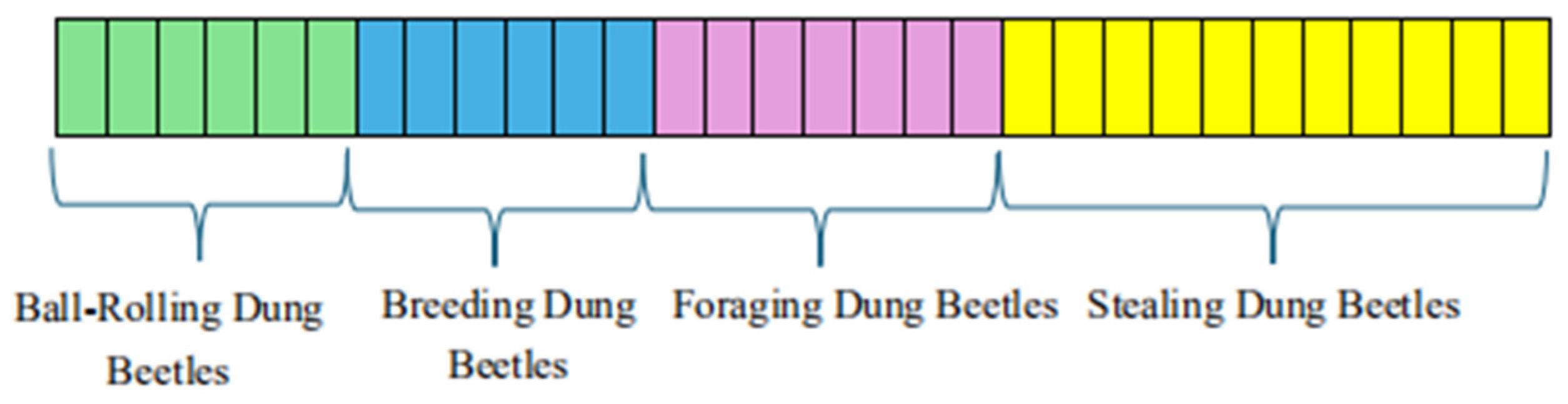
The dung beetle optimizer features a unique population structure. Based on distinct dung beetle behaviors, individuals are assigned to four different roles with a ratio of 6:6:7:11 (as illustrated in Figure 1). Each role executes specific search strategies to obtain positional information beneficial to itself. The position of each individual represents a candidate solution to the problem. When the algorithm terminates, the coordinates of the best dung beetle serve as the optimal solution.

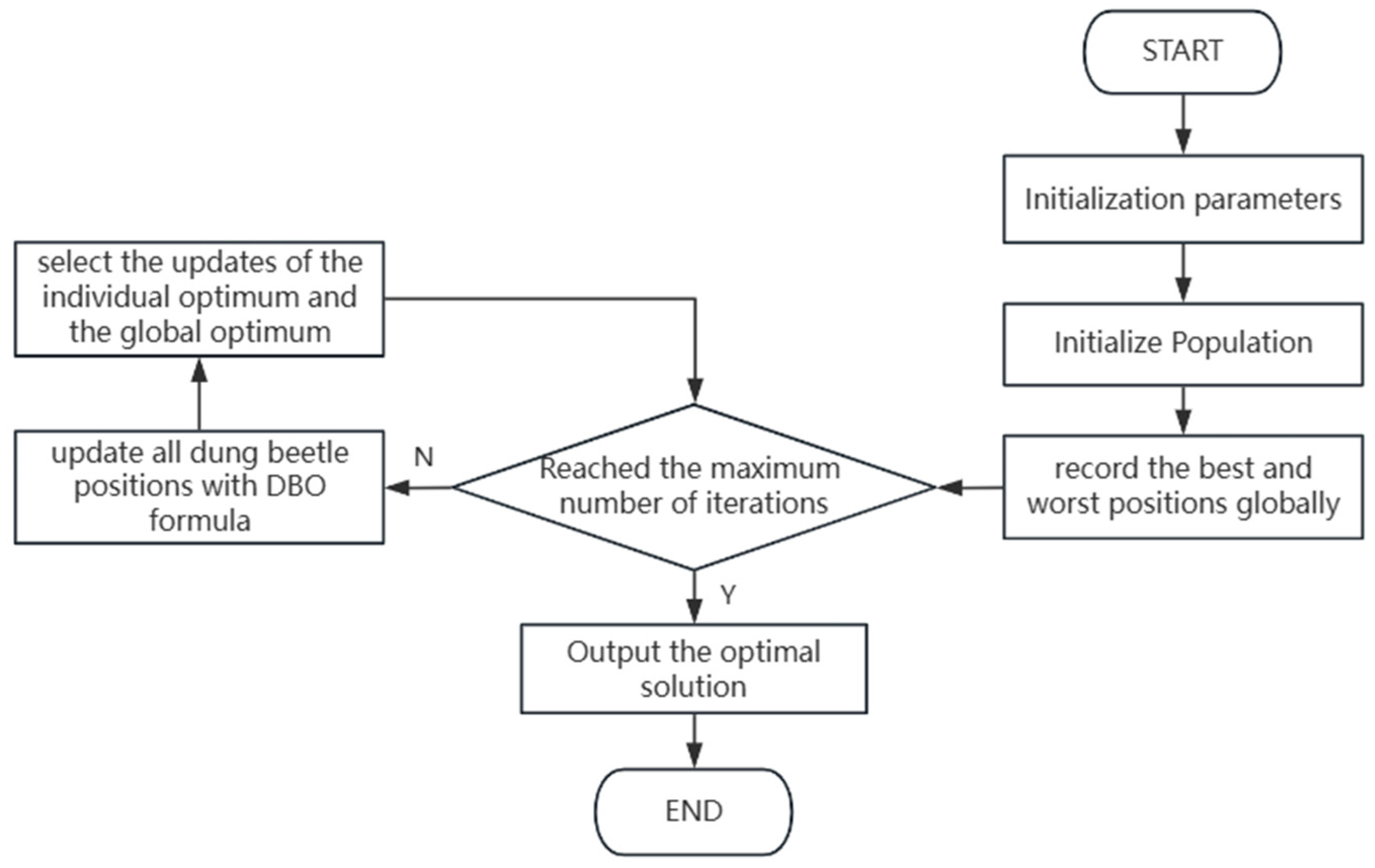
In DBO, four different kinds of beetles are mimicked, which are named ball-rolling dung beetle, breeding dung beetle, foraging dung beetle and stealing dung beetle. They behave in quite different manners, which update their positions in different expressions. The algorithm pseudocode is shown below and the flowchart is illustrated in Figure 2, where all the mathematic symbols can refer to the literature [30].

The complete pseudocode for the DBO algorithm is shown in Algorithm 1.

Algorithm 1: Dung Beetle Optimizer (DBO)
Input: pop, M, dim, lb, ub, fobj
Output: fMin, bestX
1 2 3 4 5 6 7 8 9 10 11 12 13 14 15 16 17 18 19 20 21 22 23 24 25 26 27 28 29 30 31 32 33 34 35	Begin              Initialize X randomly              Evaluate F = fobj(X)              bestX ← argmin(F), fMin ← min(F)              for t = 1 to M do                     R ← 1 − t/M                     for each rolling beetle i do                            if rand < 0.9 then                                    α ← sign(rand − 0.5)                                    Δx ← |X_i − X_worst|                                    X_i ← X_i + α·k·X_i_prev + b·Δx                            else                                    θ ← rand × π                                    X_i ← X_i + tanθ·|X_i − X_i_prev|                            end if                     end for                     Lb* ← max(bestX·(1 − R), lb)                     Ub* ← min(bestX·(1 + R), ub)                     for each breeding beetle i do                            X_i ← bestX + b1·|X_i − Lb*| + b2·|X_i − Ub*|                     end for                     Lb^b ← max(bestX·(1 − R), lb)                     Ub^b ← min(bestX·(1 + R), ub)                     for each foraging beetle i do                            X_i ← X_i + C1·(X_i − Lb^b) + C2·(X_i − Ub^b)                     end for                    for each stealing beetle i do                            X_i ← bestX + S·g·(|X_i − bestX| + |X_i − X_best|)                     end for                     Clip X_i to [lb, ub]                     Evaluate F_i = fobj(X_i)                     Update bestX, fMin              end for              return bestX, fMin        End

2.2. Particle Swarm Optimization Algorithm (PSO)

Particle swarm optimization (PSO) searches for optimal solutions through collaboration and information sharing among individual particles within a swarm. Each particle updates its position by tracking its own historical best position and the global best position found by the swarm.

The iterative update process for each particle’s velocity and position in the PSO algorithm is defined as follows:

$$v_i^{t+1}=\omega v_i^t+c_1{r}_1\left(P_i^t-x_i^t\right)+c_2{r}_2\left(P_g^t-x_i^t\right)$$

(1)

$$x_i^{t+1}=x_i^t+v_i^{t+1}$$

(2)

In Equations (1) and (2), the velocity and position of the $i$-th particle at the $t$-th iteration are denoted by $v_i^t$ and $x_i^t$. $\omega$ stands for the inertia weight. $c_1,c_2$ denote the learning factors. In the experiments, the inertia weight $\omega$ is set to 0.7, which provides a suitable balance between global exploration and local exploitation; the cognitive and social learning factors $c_1$ and $c_2$ are both set to 2.0, following the canonical PSO configuration. The values $r_1,r_2$ are uniformly distributed random numbers taken from the interval (0, 1). $P_i^t$ denotes the best position found by the $i$-th particle up to the $t$-th iteration. $P_g^t$ denotes the best position found by the entire particle swarm up to the $t$-th iteration.

2.3. Improved Dung Beetle Optimization Algorithm (DBO-PSO)

Although traditional DBO incorporates diverse search mechanisms, it still suffers from insufficient global exploration capability and a tendency to become trapped in local optima. To address these limitations, DBO-PSO introduces the Kent chaotic map and integrates the classic “velocity–position” update mechanism of PSO. In this way, the algorithm’s capacity for global exploration is strengthened, and a more favorable equilibrium between wide-ranging search and focused exploitation is attained.

2.3.1. Kent Chaotic Map

When addressing relatively complex problems, the initial population generated randomly by traditional DBO exhibits high randomness and lacks diversity, the algorithm being susceptible to getting stuck at suboptimal solutions as iterations proceed. Therefore, the Kent chaotic map is first introduced in this paper to enhance population diversity and distribution uniformity. The mathematical expression of the Kent chaotic map is as follows:

$$x_{n+1}=\left\{\begin{array}{ll}{\displaystyle \frac{x_n}{a}},& 0<x_n\le a\\ {\displaystyle \frac{1-x_n}{1-a}},& a<x_n<1\end{array}\right.$$

(3)

In Equation (3), $x_n$ denotes the chaotic variable value generated at the $n$-th iteration; $a$ denotes the control parameter, with a range of (0, 1). Compared with the Tent map and the Bernoulli–Tent map used in related DBO variants, the Kent map offers two theoretical advantages: when $a=0.4$, it achieves a strictly uniform probability density function $\rho \left(x\right)=1$ over (0, 1), whereas the Tent map has boundary discontinuities and the Bernoulli–Tent map requires an extra parameter $\epsilon$; its Lyapunov exponent is slightly higher than that of the Tent map [40], indicating marginally better ergodicity.

2.3.2. DBO-PSO Position Update Strategy

The exploration capability of traditional DBO primarily relies on the random search of stealing dung beetles and foraging dung beetles, together with the random dancing of rolling dung beetles when encountering obstacles. While this randomness contributes to exploration, it lacks clear guidance, leading to a tendency to get stuck at suboptimal solutions. By integrating the “velocity–position” update mechanism of PSO into DBO and introducing a velocity vector for each individual, the global exploration capability is significantly enhanced, thereby avoiding entrapment in local optima. The population position update formulas are as follows:

In the formulas below, $c_3$ and $c_4$ represent the proportional coefficients of DBO and PSO, respectively. In this paper, $c_3=0.5$ and $c_4=0.5$ are set. $v_i^t$ is defined in Equations (1) and (2).

The population position update formula for rolling dung beetles in obstacle-free mode is

$$x_i\left(t+1\right)=x_i\left(t\right)+c_3\left[\alpha \times k\times x_i\left(t-1\right)+b\_coef\times ∆x\right]+c_4{v}_i^t$$

(4)

In Equation (4), $x_i\left(t\right)$ denotes the position of the $i$-th dung beetle at the $t$-th iteration. $\alpha$ is a natural coefficient, where $\alpha =1$ indicates no deviation and $\alpha =-1$ indicates deviation from the original direction. $k$ denotes the deflection coefficient, with a range of $(0,0.2]$; $\mathrm{\Delta }x$ captures fluctuations in light intensity; when $\mathrm{\Delta }x$ becomes larger, the light grows weaker, which drives the dung beetle to avoid this position. $b\_coef$ represents a natural coefficient within the range (0, 1).

The population position update formula for rolling dung beetles in an obstacle encounter manner is

$$x_i\left(t+1\right)=x_i\left(t\right)+c_3\left[\tan \theta \left|x_i\left(t\right)-x_i\left(t-1\right)\right|\right]+c_4{v}_i^t$$

(5)

In Equation (5), $x_i\left(t\right)$ denotes the position of the $i$-th dung beetle at the $t$-th iteration. $\theta$ represents the deflection angle, with a range of $[0, \pi ]$. The position of the dung beetle remains unchanged when $\theta =0,\pi /2,\pi$.

For breeding dung beetles, the rule for population position is given as follows:

$$B_i\left(t+1\right)=c_3\left\{X^{*}+b_{1-vec}\times \left[B_i\left(t\right)-{Lb}^{*}\right]+b_{2-vec}\times \left[B_i\left(t\right)-{Ub}^{*}\right]\right\}+c_4{v}_i^t$$

(6)

In Equation (6), $B_i\left(t\right)$ denotes the position of the $i$-th brood ball at the $t$-th iteration. $b_{1-vec}$ and $b_{2-vec}$ represent two independent random vectors of size $1\times D$, where $D$ denotes the dimensionality of the optimization problem. $L{b}^{\mathrm{*}}$ and $U{b}^{\mathrm{*}}$ are the lower and upper bounds of the egg-laying region, respectively, and $X^{\mathrm{*}}$ is the global best position in the population.

For foraging dung beetles, the rule for updating positions is as follows:

$$x_i\left(t+1\right)=x_i\left(t\right)+c_3\left\{C_1\times \left[x_i\left(t\right)-{Lb}^b\right]+C_2\times \left[x_i\left(t\right)-{Ub}^b\right]\right\}+c_4{v}_i^t$$

(7)

In Equation (7), $C_1$ represents a random number that follows a normal distribution. $C_2$ represents a random vector with a range of (0, 1). $L{b}^b$ and $U{b}^b$ define the lower and upper bounds of the optimal foraging region.

For stealing dung beetles, the position update rule is expressed as follows:

$$x_i\left(t+1\right)=c_3\left[X^b+S\times g\times \left(\left|x_i\left(t\right)-X^{*}\right|+\left|x_i\left(t\right)-X^b\right|\right)\right]+c_4{v}_i^t$$

(8)

In Equation (8), $g$ represents a $1\times D$ random vector following a normal distribution. $S$ denotes a constant. $X^b$ represents the current best position. $X^{\mathrm{*}}$ denotes the global best position of the population.

2.3.3. DBO-PSO Algorithm Pseudocode and Flowchart

The complete pseudocode for the DBO-PSO algorithm is shown in Algorithm 2.

Algorithm 2: Improved Dung Beetle Optimizer (DBO-PSO)
Input: pop, M, dim, lb, ub, fobj
Output: bestX, fMin
1 2 3 4 5 6 7 8 9 10 11 12 13 14 15 16 17 18 19 20 21 22 23 24 25 26 27 28 29 30 31 32 33 34 35 36 37 38 39 40 41 42 43 44	Begin                Initialize X using Kent chaotic map                Initialize V randomly                Evaluate F = fobj(X)                pX ← X, pFit ← F                bestX ← argmin(F), fMin ← min(F)                        for t = 1 to M do                        R ← 1 − t/M                                        for each rolling beetle i do                                Update V_i                                if rand < 0.9 then                                        Δx ← |X_i − X_worst|                                        X_dbo ← X_i + α·k·X_i_prev + b_coef·Δx                                else                                        θ ← rand × π                                        X_dbo ← X_i + tanθ·|X_i − pX_i|                                end if                                X_i ← X_i + c3·(X_dbo − X_i) + c4·V_i                        end for                        Lb* ← max(bestX·(1 − R), lb)                        Ub* ← min(bestX·(1 + R), ub)                        for each breeding beetle i do                                Update V_i                                X_dbo ← bestX + b1-vec·|X_i − Lb*| + b2-vec·|X_i − Ub*|                                X_i ← X_i + c3·(X_dbo − X_i) + c4·V_i                        end for                       Lb^b ← max(bestX·(1 − R), lb)                        Ub^b ← min(bestX·(1 + R), ub)                        for each foraging beetle i do                                Update V_i                                X_dbo ← X_i + C1·(X_i − Lb^b) + C2·(X_i − Ub^b)                                X_i ← X_i + c3·(X_dbo − X_i) + c4·V_i                        end for                        for each stealing beetle i do                                Update V_i                                X_dbo ← bestX + S·g·(|X_i − bestX| + |X_i − pX_i|)                                X_i ← X_i + c3·(X_dbo − X_i) + c4·V_i                        end for                        Clip X_i to [lb, ub]                        Evaluate F_i = fobj(X_i)                        Update pX_i, pFit_i, bestX, fMin                 end for                return bestX, fMin         End

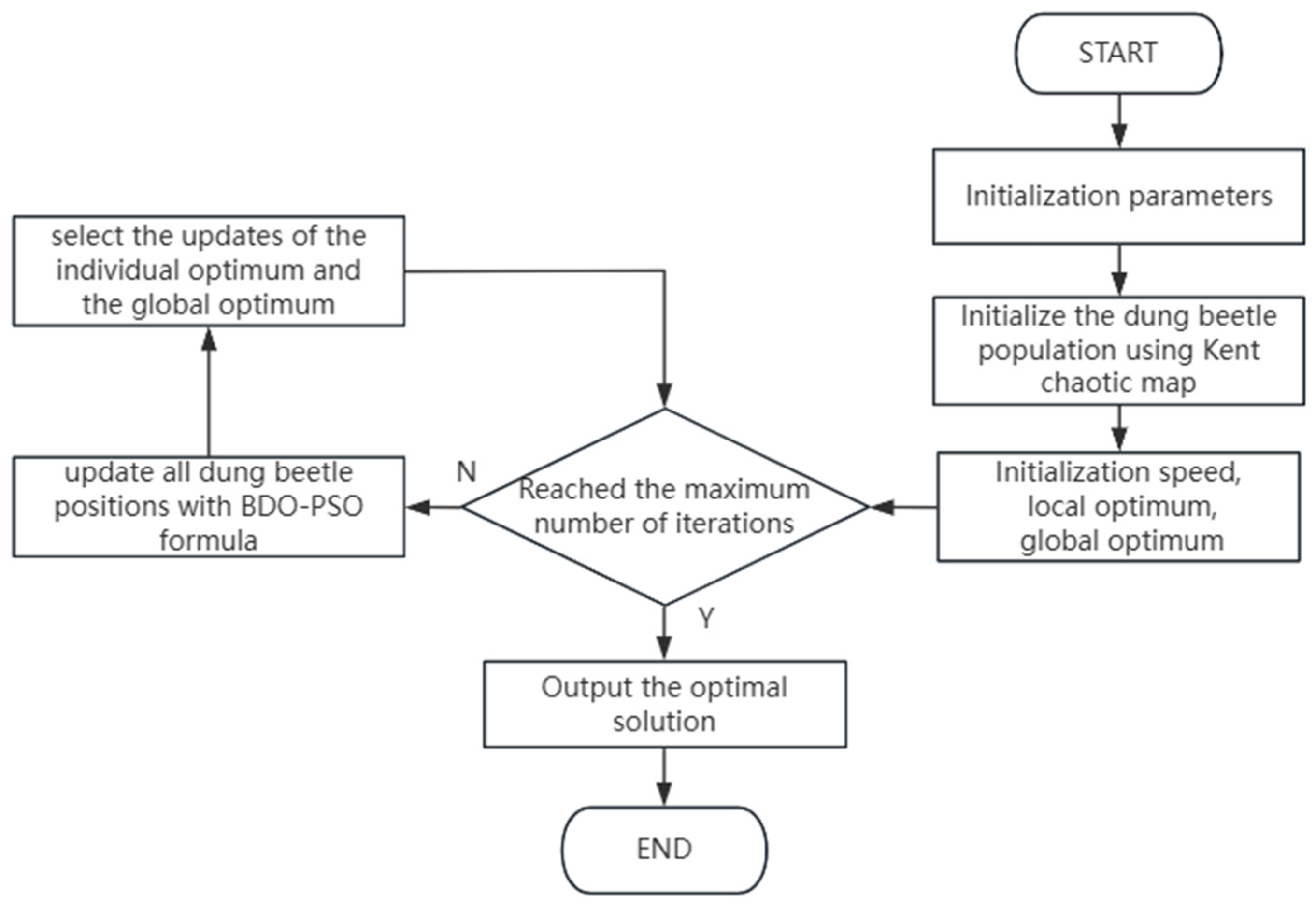
The DBO-PSO algorithm flow is shown in Figure 3.

3. CEC 2022 Benchmark Functions Verification

To verify the effectiveness of the proposed DBO-PSO algorithm, several classical and advanced swarm intelligence algorithms are selected for comparison, including the dung beetle optimizer (DBO), the improved dung beetle optimizer (IDBO), environment-aware chaotic force-field dung beetle optimizer (ECFDBO), particle swarm optimization (PSO), Sparrow Search Algorithm (SSA), whale optimization algorithm (WOA), differential evolution (DE), and genetic algorithm (GA). The parameter settings of the nine algorithms are shown in

Table 1. Compare the relevant parameters of algorithms.

Algorithms	Parameters
DBO-PSO	$w=0.7,c_1=2,c_2=2,c_3=0.5,c_4=0.5,a=0.4$
IDBO	$k=0.5,b=0.3,S=0.3$
ECFDBO	$p=0.2,w=0.5,pm=0.07$
DBO	$\mathrm{k}\in (0,0.2],b\_coef\in (0,1),\theta \in [0,\pi ]$
PSO	$w=0.7,c_1=2,c_2=2$
DE	$F=0.5,CR=0.5$
SSA	$p_{\mathrm{percent}}=0.2,{\mathrm{r}}_{\mathrm{percent}}=0.1,ST=0.8$
WOA	$\mathrm{a}=2\to 0,b=1,l\in [-1,1]$
GA	$pc=0.6,pm=0.3$

. Comparative experiments are conducted on 12 benchmark functions from the CEC2022-20D test suite, as listed in

Table 2. CEC2022-20D test set.

	No.	Functions	Fi
Unimodal Function	1	Shifted and full Rotated Zakharov Function (Modified f2, CEC 2017)	300
Basic Functions	2	Shifted and full Rotated Rosenbrock’s Function (Modified f3, CEC 2017)	400
	3	Shifted and full Rotated Expanded Schaffer’s f6 Function (Modified f5, CEC 2017)	600
	4	Shifted and full Rotated Non-Continuous Rastrigin’s Function (Modified f7, CEC 2017)	800
	5	Shifted and full Rotated Levy Function (Modified f8, CEC 2017)	900
Hybrid Functions	6	Hybrid Function 1 (N = 3) (f18, CEC 2014 )	1800
	7	Hybrid Function 2 (N = 6) (f19, CEC 2017)	2000
	8	Hybrid Function 3 (N = 5) (f22, CEC 2014)	2200
Composition Functions	9	Composition Function 1 (N = 5) (f23, CEC 2014)	2300
	10	Composition Function 2 (N = 4) (f24, CEC 2014)	2400
	11	Composition Function 3 (N = 5) (f25, CEC 2017)	2600
	12	Composition Function 4 (N = 6) (f26, CEC 2017)	2700

along with their theoretical optimal values. Among them, F1 is a unimodal function, which is mainly used to evaluate the convergence speed and optimization accuracy of the algorithms. F2 to F5 are basic multimodal functions, primarily adopted to test the global exploration capability and the ability to escape local optima. F6 to F8 are hybrid functions constructed by combining multiple sub-functions, which can evaluate the algorithm’s ability to handle problems with mixed properties. F9 to F12 are composition functions that integrate different types of basic functions, comprehensively testing the solution accuracy, stability, and robustness of each algorithm for complex optimization problems.

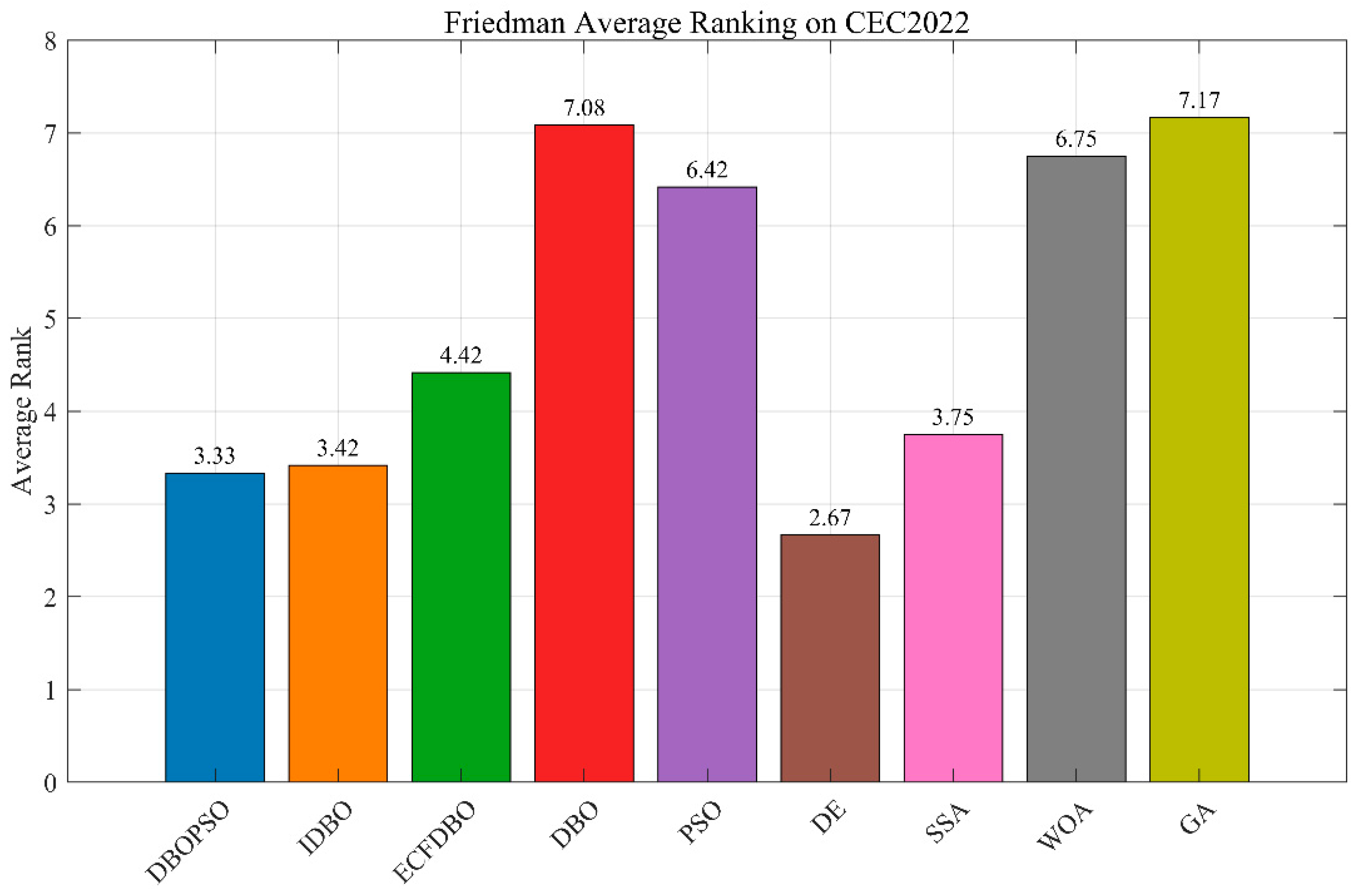
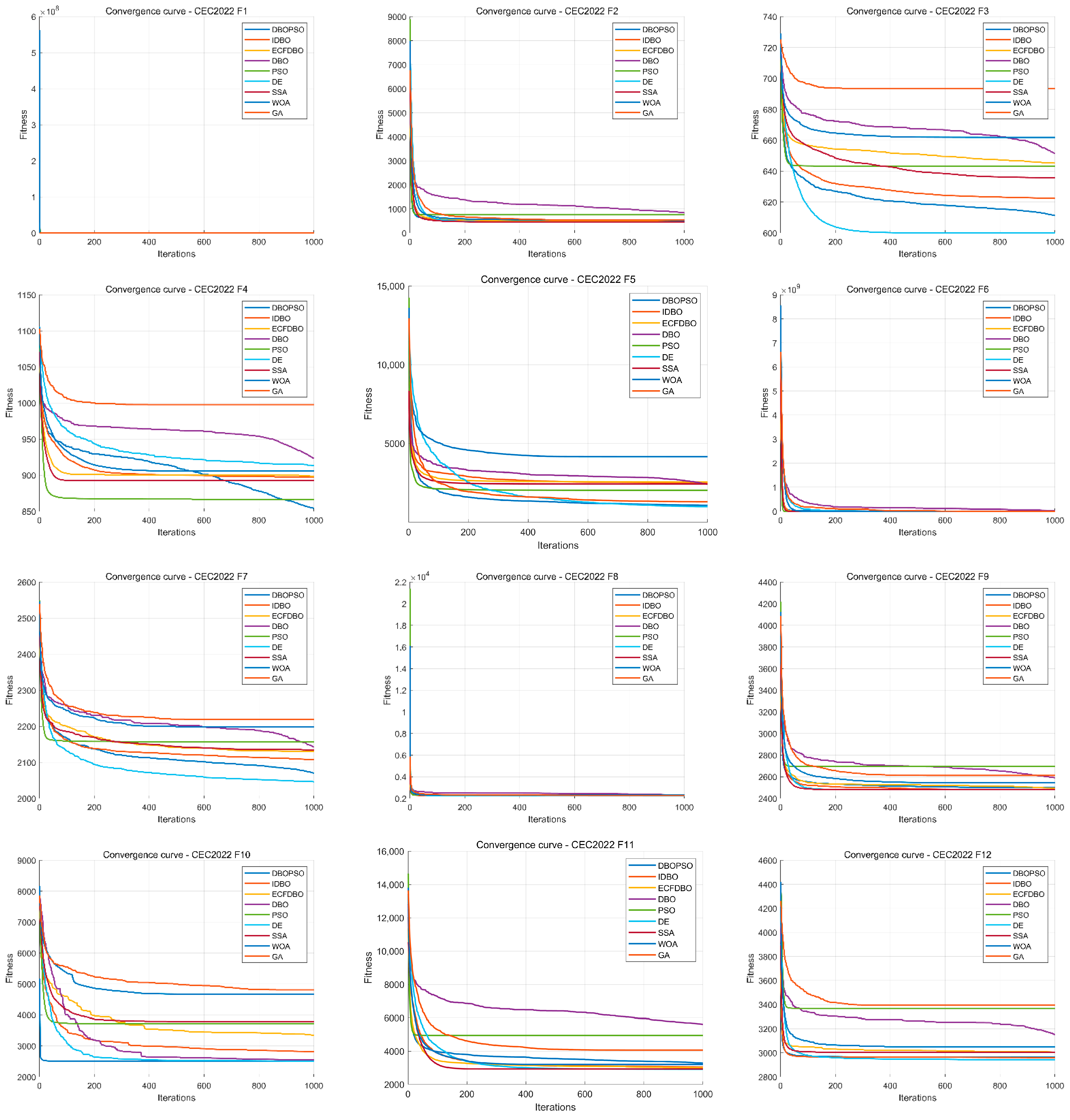
All experiments are performed under the Windows 10 operating system, running on hardware with a quad-core eight-thread 2.40 GHz Intel(R) Core (TM) i5-10200H CPU, 16 GB of RAM, and an NVIDIA GeForce GTX 1650 (4 GB) graphics card, with MATLAB R2024b used as the programming software. For all comparative algorithms, the population size is uniformly set to 50, the maximum number of iterations is set to 1000 with a dimensionality of 20, and each test function is run independently 30 times to ensure statistical significance. Six evaluation metrics are adopted to comprehensively assess the algorithm performance, including the minimum, average, median, maximum, standard deviation, and average running time. The experimental results are presented in

Table 3. Test results.

Fun	Index	DBO-PSO	IDBO	ECFDBO	DBO	PSO	DE	SSA	WOA	GA
F1	min	4.039 × 102	6.048 × 102	3.133 × 102	1.187 × 104	8.772 × 103	2.389 × 104	3.412 × 102	8.644 × 103	3.281 × 104
	std	7.312 × 102	2.454 × 103	2.838 × 102	5.676 × 103	9.808 × 103	4.511 × 103	1.211 × 103	4.696 × 103	2.135 × 104
	avg	1.773 × 103	3.047 × 103	5.936 × 102	2.489 × 104	2.744 × 104	3.291 × 104	1.950 × 103	1.539 × 104	8.007 × 104
	median	1.494 × 103	2.240 × 103	4.863 × 102	2.578 × 104	2.600 × 104	3.317 × 104	1.651 × 103	1.461 × 104	8.051 × 104
	worse	3.726 × 103	9.490 × 103	1.345 × 103	3.457 × 104	5.593 × 104	4.114 × 104	5.118 × 103	2.782 × 104	1.145 × 105
	avg_time	2.113 × 10−1	1.574 × 10−1	7.128 × 10−1	3.944 × 10−1	2.460 × 10−1	6.989 × 10−1	3.979 × 10−1	2.061 × 10−1	2.436 × 10−1
F2	min	4.348 × 102	4.098 × 102	4.067 × 102	6.626 × 102	5.853 × 102	4.451 × 102	4.015 × 102	4.541 × 102	4.889 × 102
	std	5.615 × 101	3.459 × 101	2.798 × 101	1.255 × 102	1.102 × 102	1.261 × 100	1.896 × 101	5.280 × 101	3.718 × 101
	avg	5.026 × 102	4.599 × 102	4.630 × 102	8.356 × 102	7.542 × 102	4.488 × 102	4.503 × 102	5.462 × 102	5.342 × 102
	median	4.858 × 102	4.492 × 102	4.503 × 102	8.292 × 102	7.507 × 102	4.491 × 102	4.491 × 102	5.463 × 102	5.208 × 102
	worse	6.885 × 102	5.785 × 102	5.616 × 102	1.201 × 103	9.673 × 102	4.518 × 102	4.747 × 102	6.391 × 102	6.369 × 102
	Avg_time	3.267 × 10−1	2.776 × 10−1	1.488 × 100	4.470 × 10−1	2.269 × 10−1	9.324 × 10−1	4.623 × 10−1	1.937 × 10−1	2.766 × 10−1
F3	min	6.022 × 102	6.021 × 102	6.207 × 102	6.363 × 102	6.261 × 102	6.000 × 102	6.141 × 102	6.432 × 102	6.602 × 102
	std	5.749 × 100	1.323 × 101	1.343 × 101	6.898 × 100	1.063 × 101	1.311 × 10−5	1.183 × 101	1.246 × 101	1.456 × 101
	avg	6.112 × 102	6.223 × 102	6.452 × 102	6.512 × 102	6.432 × 102	6.000 × 102	6.357 × 102	6.619 × 102	6.936 × 102
	median	6.107 × 102	6.215 × 102	6.459 × 102	6.515 × 102	6.410 × 102	6.000 × 102	6.349 × 102	6.582 × 102	6.944 × 102
	worse	6.288 × 102	6.517 × 102	6.717 × 102	6.696 × 102	6.663 × 102	6.000 × 102	6.553 × 102	6.891 × 102	7.216 × 102
	avg_time	5.344 × 10−1	4.736 × 10−1	3.583 × 100	6.041 × 10−1	4.126 × 10−1	1.182 × 100	7.817 × 10−1	3.905 × 10−1	4.877 × 10−1
F4	min	8.198 × 102	8.557 × 102	8.603 × 102	9.020 × 102	8.395 × 102	8.944 × 102	8.534 × 102	8.671 × 102	9.565 × 102
	std	1.840 × 101	2.293 × 101	2.876 × 101	1.292 × 101	1.553 × 101	8.496 × 100	2.001 × 101	2.725 × 101	1.595 × 101
	avg	8.539 × 102	8.973 × 102	8.983 × 102	9.229 × 102	8.662 × 102	9.134 × 102	8.923 × 102	9.056 × 102	9.978 × 102
	median	8.535 × 102	8.964 × 102	8.967 × 102	9.233 × 102	8.635 × 102	9.121 × 102	8.915 × 102	9.020 × 102	9.992 × 102
	worse	8.995 × 102	9.488 × 102	9.900 × 102	9.504 × 102	9.090 × 102	9.342 × 102	9.502 × 102	9.824 × 102	1.036 × 103
	avg_time	3.699 × 10−1	3.410 × 10−1	1.706 × 100	5.048 × 10−1	3.105 × 10−1	8.849 × 10−1	6.277 × 10−1	2.645 × 10−1	3.323 × 10−1
F5	min	9.042 × 102	1.558 × 103	1.546 × 103	1.888 × 103	1.349 × 103	9.276 × 102	1.823 × 103	2.136 × 103	9.281 × 102
	std	1.891 × 102	4.123 × 102	6.751 × 102	3.008 × 102	4.265 × 102	3.574 × 101	2.005 × 102	1.563 × 103	7.179 × 102
	avg	1.054 × 103	2.478 × 103	2.552 × 103	2.401 × 103	2.010 × 103	9.764 × 102	2.412 × 103	4.153 × 103	1.294 × 103
	median	9.954 × 102	2.463 × 103	2.406 × 103	2.429 × 103	1.924 × 103	9.675 × 102	2.419 × 103	3.969 × 103	9.947 × 102
	worse	1.688 × 103	3.230 × 103	4.560 × 103	3.066 × 103	2.936 × 103	1.061 × 103	2.823 × 103	7.777 × 103	3.863 × 103
	avg_time	3.861 × 10−1	3.185 × 10−1	1.316 × 100	5.071 × 10−1	3.158 × 10−1	9.486 × 10−1	5.131 × 10−1	1.518 × 10−1	1.954 × 10−1
F6	min	1.274 × 104	2.133 × 103	2.119 × 103	2.158 × 106	1.946 × 103	6.183 × 105	1.853 × 103	7.168 × 103	2.652 × 103
	std	7.393 × 106	9.095 × 103	2.753 × 104	1.985 × 107	4.525 × 105	1.088 × 106	5.854 × 103	2.066 × 105	1.254 × 104
	avg	2.233 × 106	1.126 × 104	1.955 × 104	3.149 × 107	1.022 × 105	2.219 × 106	6.933 × 103	1.273 × 105	1.189 × 104
	median	8.734 × 104	7.263 × 103	9.857 × 103	2.641 × 107	5.191 × 103	1.844 × 106	4.604 × 103	5.621 × 104	6.930 × 103
	worse	2.938 × 107	2.630 × 104	1.221 × 105	7.028 × 107	2.483 × 106	5.343 × 106	2.009 × 104	1.035 × 106	6.721 × 104
	avg_time	1.862 × 10−1	1.574 × 10−1	1.114 × 100	2.473 × 10−1	1.456 × 10−1	4.929 × 10−1	2.838 × 10−1	1.176 × 10−1	1.604 × 10−1
F7	min	2.033 × 103	2.034 × 103	2.055 × 103	2.114 × 103	2.066 × 103	2.034 × 103	2.031 × 103	2.111 × 103	2.142 × 103
	std	2.698 × 101	4.821 × 101	4.906 × 101	1.785 × 101	5.897 × 101	7.231 × 100	8.704 × 101	5.240 × 101	4.450 × 101
	avg	2.070 × 103	2.108 × 103	2.130 × 103	2.143 × 103	2.157 × 103	2.046 × 103	2.134 × 103	2.199 × 103	2.219 × 103
	median	2.061 × 103	2.100 × 103	2.125 × 103	2.143 × 103	2.149 × 103	2.046 × 103	2.125 × 103	2.186 × 103	2.225 × 103
	worse	2.142 × 103	2.210 × 103	2.250 × 103	2.180 × 103	2.280 × 103	2.060 × 103	2.485 × 103	2.315 × 103	2.303 × 103
	avg_time	3.457 × 10−1	3.146 × 10−1	4.061 × 100	6.818 × 10−1	4.798 × 10−1	1.128 × 100	8.189 × 10−1	4.325 × 10−1	3.653 × 10−1
F8	min	2.230 × 103	2.224 × 103	2.227 × 103	2.231 × 103	2.226 × 103	2.227 × 103	2.222 × 103	2.233 × 103	2.235 × 103
	std	3.904 × 101	2.966 × 101	5.716 × 101	9.528 × 101	9.285 × 101	6.729 × 10−1	6.230 × 101	5.913 × 101	5.198 × 101
	avg	2.259 × 103	2.240 × 103	2.282 × 103	2.318 × 103	2.302 × 103	2.228 × 103	2.286 × 103	2.293 × 103	2.283 × 103
	median	2.247 × 103	2.228 × 103	2.249 × 103	2.266 × 103	2.239 × 103	2.228 × 103	2.255 × 103	2.259 × 103	2.255 × 103
	worse	2.368 × 103	2.343 × 103	2.369 × 103	2.526 × 103	2.571 × 103	2.230 × 103	2.461 × 103	2.408 × 103	2.383 × 103
	avg_time	3.902 × 10−1	3.606 × 10−1	3.443 × 100	4.768 × 10−1	3.528 × 10−1	7.489 × 10−1	5.763 × 10−1	3.276 × 10−1	4.293 × 10−1
F9	min	2.481 × 103	2.481 × 103	2.481 × 103	2.514 × 103	2.571 × 103	2.481 × 103	2.481 × 103	2.483 × 103	2.560 × 103
	std	3.908 × 101	1.445 × 10−1	2.954 × 101	3.383 × 101	8.115 × 101	4.458 × 10−5	2.411 × 10−2	5.115 × 101	2.760 × 101
	avg	2.502 × 103	2.481 × 103	2.492 × 103	2.591 × 103	2.697 × 103	2.481 × 103	2.481 × 103	2.547 × 103	2.612 × 103
	median	2.481 × 103	2.481 × 103	2.481 × 103	2.594 × 103	2.686 × 103	2.481 × 103	2.481 × 103	2.529 × 103	2.618 × 103
	worse	2.654 × 103	2.481 × 103	2.622 × 103	2.657 × 103	2.926 × 103	2.481 × 103	2.481 × 103	2.675 × 103	2.662 × 103
	avg_time	4.255 × 10−1	3.766 × 10−1	4.799 × 100	8.240 × 10−1	5.243 × 10−1	1.258 × 100	9.993 × 10−1	4.335 × 10−1	6.012 × 10−1
F10	min	2.501 × 103	2.501 × 103	2.501 × 103	2.522 × 103	2.512 × 103	2.501 × 103	2.501 × 103	2.501 × 103	2.542 × 103
	std	2.381 × 100	4.170 × 102	9.467 × 102	1.989 × 101	1.031 × 103	1.031 × 101	7.582 × 102	1.191 × 103	1.367 × 103
	avg	2.502 × 103	2.814 × 103	3.347 × 103	2.547 × 103	3.718 × 103	2.513 × 103	3.780 × 103	4.671 × 103	4.810 × 103
	median	2.501 × 103	2.501 × 103	3.029 × 103	2.541 × 103	4.030 × 103	2.512 × 103	3.834 × 103	4.933 × 103	5.367 × 103
	worse	2.509 × 103	3.752 × 103	5.828 × 103	2.625 × 103	5.410 × 103	2.548 × 103	5.007 × 103	6.259 × 103	6.246 × 103
	avg_time	5.596 × 10−1	4.724 × 10−1	4.704 × 100	6.223 × 10−1	4.190 × 10−1	1.152 × 100	7.726 × 10−1	4.682 × 10−1	4.754 × 10−1
F11	min	2.949 × 103	2.608 × 103	2.600 × 103	4.672 × 103	4.150 × 103	2.900 × 103	2.900 × 103	2.770 × 103	3.552 × 103
	std	3.664 × 102	1.829 × 102	4.019 × 102	4.239 × 102	5.003 × 102	2.203 × 101	4.498 × 101	1.877 × 102	2.992 × 102
	avg	3.277 × 103	3.046 × 103	3.004 × 103	5.612 × 103	4.944 × 103	2.906 × 103	2.927 × 103	3.201 × 103	4.062 × 103
	median	3.123 × 103	2.971 × 103	2.900 × 103	5.667 × 103	4.970 × 103	2.900 × 103	2.900 × 103	3.161 × 103	4.075 × 103
	worse	4.093 × 103	3.303 × 103	4.970 × 103	6.491 × 103	5.704 × 103	3.019 × 103	3.000 × 103	3.646 × 103	4.670 × 103
	avg_time	7.305 × 10−1	7.432 × 10−1	4.846 × 100	8.816 × 10−1	6.576 × 10−1	1.343 × 100	1.076 × 100	6.423 × 10−1	7.725 × 10−1
F12	min	2.941 × 103	2.939 × 103	2.957 × 103	2.988 × 103	3.189 × 103	2.937 × 103	2.943 × 103	2.971 × 103	3.143 × 103
	std	1.766 × 101	1.747 × 101	4.783 × 101	7.839 × 101	1.523 × 102	2.022 × 100	5.834 × 101	6.465 × 101	1.374 × 102
	avg	2.963 × 103	2.961 × 103	3.006 × 103	3.151 × 103	3.369 × 103	2.942 × 103	3.004 × 103	3.048 × 103	3.395 × 103
	median	2.958 × 103	2.957 × 103	2.989 × 103	3.148 × 103	3.321 × 103	2.942 × 103	2.987 × 103	3.034 × 103	3.370 × 103
	worse	3.029 × 103	3.028 × 103	3.171 × 103	3.315 × 103	3.893 × 103	2.945 × 103	3.186 × 103	3.237 × 103	3.695 × 103
	avg_time	7.896 × 10−1	8.327 × 10−1	9.349 × 100	5.572 × 10−1	4.229 × 10−1	8.092 × 10−1	6.700 × 10−1	4.009 × 10−1	4.435 × 10−1

,

Table 4. Wilcoxon rank-sum test.

Fun	IDBO	ECFDBO	DBO	PSO	DE	SSA	WOA	GA
F1	2.510 × 10−2	3.020 × 10−11	3.020 × 10−11	3.020 × 10−11	3.020 × 10−11	1.953 × 10−3	3.338 × 10−11	3.020 × 10−11
F2	1.221 × 10−2	3.020 × 10−11	3.690 × 10−11	1.094 × 10−10	1.108 × 10−6	8.120 × 10−4	4.084 × 10−5	8.883 × 10−6
F3	2.959 × 10−5	3.018 × 10−11	3.020 × 10−11	3.020 × 10−11	3.020 × 10−11	2.922 × 10−9	3.020 × 10−11	3.020 × 10−11
F4	1.635 × 10−5	3.018 × 10−11	3.020 × 10−11	5.012 × 10−2	7.389 × 10−11	2.598 × 10−8	2.602 × 10−8	3.020 × 10−11
F5	3.159 × 10−10	3.020 × 10−11	1.206 × 10−10	3.820 × 10−10	3.478 × 10−1	3.159 × 10−10	4.077 × 10−11	5.997 × 10−1
F6	1.329 × 10−10	3.012 × 10−11	1.287 × 10−9	1.202 × 10−8	3.256 × 10−7	3.338 × 10−11	6.843 × 10−1	5.573 × 10−10
F7	6.145 × 10−2	3.020 × 10−11	2.922 × 10−9	1.695 × 10−9	2.377 × 10−7	5.828 × 10−3	1.957 × 10−10	1.094 × 10−10
F8	1.861 × 10−6	3.018 × 10−11	5.746 × 10−2	7.172 × 10−1	3.020 × 10−11	5.895 × 10−1	5.395 × 10−1	1.273 × 10−2
F9	1.070 × 10−9	3.020 × 10−11	1.695 × 10−9	3.690 × 10−11	3.020 × 10−11	3.330 × 10−11	6.203 × 10−4	7.389 × 10−11
F10	5.874 × 10−4	3.018 × 10−11	3.020 × 10−11	4.504 × 10−11	2.254 × 10−4	1.957 × 10−10	2.610 × 10−10	3.020 × 10−11
F11	3.632 × 10−1	3.020 × 10−11	3.020 × 10−11	3.020 × 10−11	3.020 × 10−11	3.564 × 10−4	2.959 × 10−5	3.020 × 10−11
F12	1.580 × 10−1	3.012 × 10−11	1.613 × 10−10	3.338 × 10−11	8.153 × 10−11	1.518 × 10−3	4.311 × 10−8	3.020 × 10−11

and

Table 5. Friedman statistical results.

Fun	DBO-PSO	IDBO	ECFDBO	DBO	PSO	DE	SSA	WOA	GA
Mean Rank	3.33	3.42	4.42	7.08	6.42	2.67	3.75	6.75	7.17

. The average ranking of the nine algorithms is visualized in Figure 4, and their convergence curves on the benchmark functions are shown in Figure 5.

As shown in the statistical tables, DBO-PSO demonstrates competitive performance across all benchmark functions. For the unimodal function F1, which evaluates convergence speed and optimization accuracy, DBO-PSO achieves an average value at 1773.0, significantly outperforming DBO at 24,890.0, PSO at 27,440.0, and GA at 80,070.0. Only IDBO and ECFDBO yield better results, indicating that DBO-PSO possesses favorable convergence precision on unimodal problems.

For basic multimodal functions F2 to F5, which test global exploration capability and the ability to escape local optima, DBO-PSO consistently ranks among the top performers. On F2, DBO-PSO obtains a mean at 502.6, superior to DBO, PSO, WOA, and GA. On F5, DBO-PSO achieves a mean at 1054.0, again outperforming the same four algorithms. These results confirm that DBO-PSO possesses strong local search capability and robustness when handling complex multimodal problems.

For hybrid functions F6 to F8, which evaluate the ability to handle problems with mixed properties, DBO-PSO maintains stable performance. On F7 and F8, DBO-PSO outperforms DBO, PSO, WOA, and GA, demonstrating its effectiveness in balancing global exploration and local exploitation.

For composition functions F9 to F12, which test solution accuracy and stability on complex problems, DBO-PSO also shows competitive advantages. On F10, DBO-PSO achieves a mean at 2502.0 with an extremely low standard deviation at 2.38, outperforming all algorithms except DE. On F12, DBO-PSO obtains a mean at 2963.0, outperforming DBO, PSO, WOA, and GA. This demonstrates that DBO-PSO possesses accurate global search ability and superior robustness on composition functions.

To further evaluate the performance differences, the Wilcoxon rank-sum test is conducted. As shown in Table 4, DBO-PSO achieves statistically significant differences against DBO on all 12 functions and against PSO on 11 functions. According to the Friedman test in Table 5, DBO-PSO achieves an average rank at 3.33, placing it second among all compared algorithms, behind DE at 2.67 and ahead of DBO at 7.08 and PSO at 6.42. The Friedman test indicates statistically significant differences among the algorithms.

In conclusion, the integration of Kent chaotic mapping and the PSO velocity–position update mechanism effectively enhances population diversity and global search capability, making DBO-PSO a competitive optimizer for complex optimization problems.

4. Path Planning Experiments and Results Analysis

4.1. Experimental Environment Setup

4.1.1. Experimental Platform and Software

To validate the effectiveness of the DBO-PSO algorithm proposed in this paper for UAV path planning in complex three-dimensional environments, a three-dimensional experimental city is constructed to emulate a UAV path planning environment, and experiments are conducted. All experiments are performed under the Windows 10 operating system, running on hardware with a quad-core eight-thread 2.40 GHz Intel(R) Core (TM) i5-10200H CPU, 16 GB of RAM, and an NVIDIA GeForce GTX 1650 (4 GB) graphics card. MATLAB R2024b is used as the programming software.

4.1.2. 3D Simulated City Model

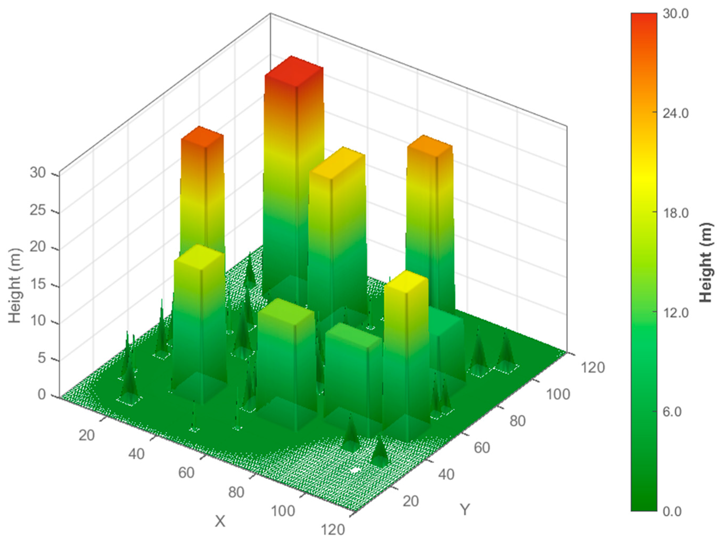
In the study of UAV path planning technology, a high-quality experimental environment serves as a crucial prerequisite for algorithm validation. Therefore, a three-dimensional experimental city model is constructed on MATLAB (as shown in Figure 6). In this experimental environment, a three-dimensional Cartesian coordinate system is established with a 120 × 120 × 30 grid map. The value ranges of the X, Y and Z coordinates are limited to 0–120 m, 0–120 m and 0–30 m, respectively. The model includes various types of structures to simulate real-world urban elements such as commercial buildings, industrial buildings, residential structures, and trees. Buildings are represented as cuboids, while trees are represented as cones. Both are defined using a binary obstacle mask and a height matrix.

The coordinates of the buildings are defined as [x₀, y₀, width, length, height], where the pair (x₀, y₀) denotes the starting coordinates of the upper-left corner of the building, width denotes the length along the X-axis, and length denotes the length along the Y-axis. The building height represents the vertical dimension along the Z-axis. A total of nine buildings with different dimensions are generated. The parameter settings of the building obstacles are shown in

Table 6. Parameters of architectural obstacles.

X-Axis Origin	Y-Axis Origin	Building Width (m)	Building Length (m)	Building Height (m)
30	25	12	14	18
80	40	18	9	12
45	80	10	20	22
90	70	15	15	9
15	50	11	11	28
60	30	16	12	14
100	45	10	13	20
20	90	14	16	30
70	100	13	10	25

.

The positions of trees are randomly generated, ensuring the avoidance of existing buildings and road areas. Each tree occupies a grid size ranging from 1 × 1 to 3 × 3, with heights varying between 4 and 8 m. Herein, 40 trees are generated.

This experimental setup employs a total of five intermediate waypoints. The starting point is located at [10, 110, 10] in the urban fringe area, and the endpoint is located at [110, 10, 10] in the diagonal region. The planned path must avoid all obstacles while satisfying safe flight requirements. It is worth emphasizing that the current experiments are conducted on a simulated urban environment as a proof of concept, and the algorithm shows good potential for extension to real-world applications by incorporating georeferenced urban data in future studies.

4.2. Path Planning Experiment

4.2.1. UAV Path Planning Model

For cost components, they are assigned respective weight and aggregated to form the total path cost function. Its mathematical expression is formulated as follows:

$$F_{cost}=b_1{f}_l+b_2{f}_s+b_3{f}_c+b_4{f}_h$$

(9)

In Equation (9), $F_{\cos \mathrm{t}}$ denotes the total path cost function. $b_1,b_2,b_3,b_4$ represent the weight for the path length cost, path smoothness cost, collision threat cost, and flight altitude cost, respectively. A smaller value of $F_{\cos \mathrm{t}}$ indicates a higher quality of the path obtained from the algorithm. Different weight values inevitably lead to variations in the path planning results, making it challenging to achieve the theoretically optimal weight combination. Furthermore, for different practical applications, different weighting priorities can be adopted—for instance, when focusing on fuel consumption or green trajectory planning, a higher weight can be assigned to altitude. The individual cost models and weight values used in the current paper are adopted in the previously published literature from our team [25].

4.2.2. Algorithm Parameter Configuration

In this experiment, the effectiveness of DBO-PSO is verified using different population sizes, while all other parameters remain consistent. A systematic comparison between DBO-PSO and four other algorithms, namely DBO, PSO, IDBO, and ECFDBO, is conducted based on metrics such as the path length cost, smoothness cost, flight altitude cost and collision threat cost. Path diagrams of DBO-PSO and DBO are also plotted to visually demonstrate the trajectories planned by the two algorithms. The maximum iteration count is configured as 500, with five intermediate waypoints specified. A safety buffer of 2 m is adopted, and the flight altitude is limited between 5 m at the lower bound and 100 m at the upper bound. With all other parameters unchanged, comparative experiments are conducted for three different population scales—small, medium, and large—with each group of experiments repeated 30 times to eliminate random errors and enhance the credibility of the results. The small-scale population size is set to 50, the medium-scale population size is set to 100, and the large scale is set to 150.

4.2.3. Experimental Results Presentation

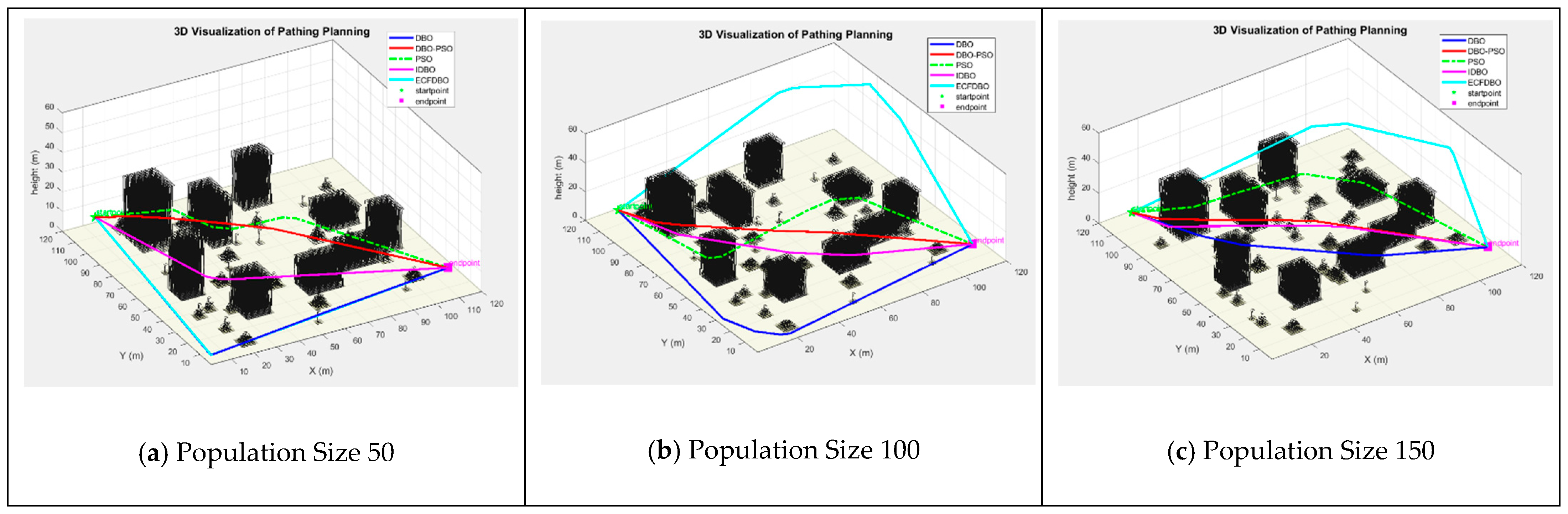
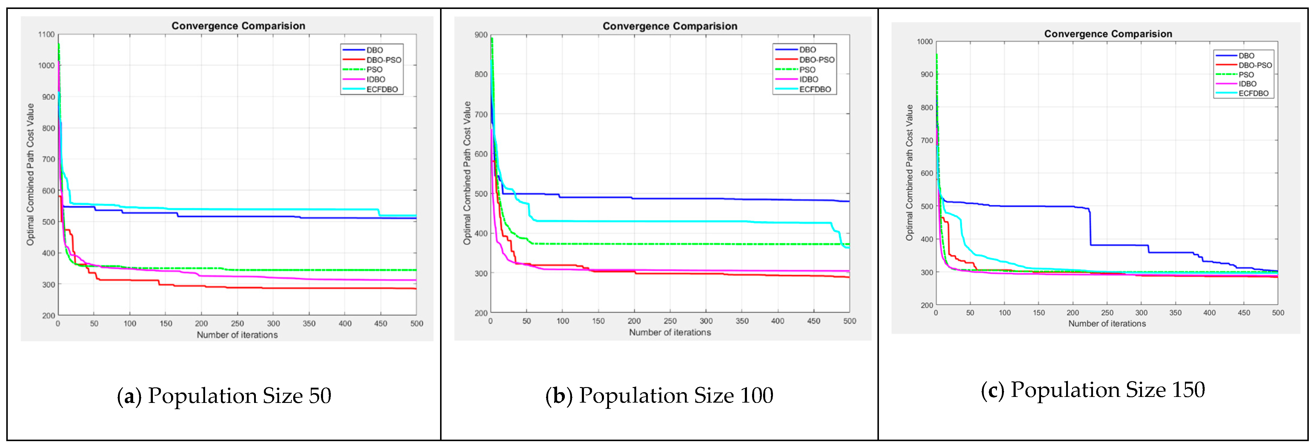
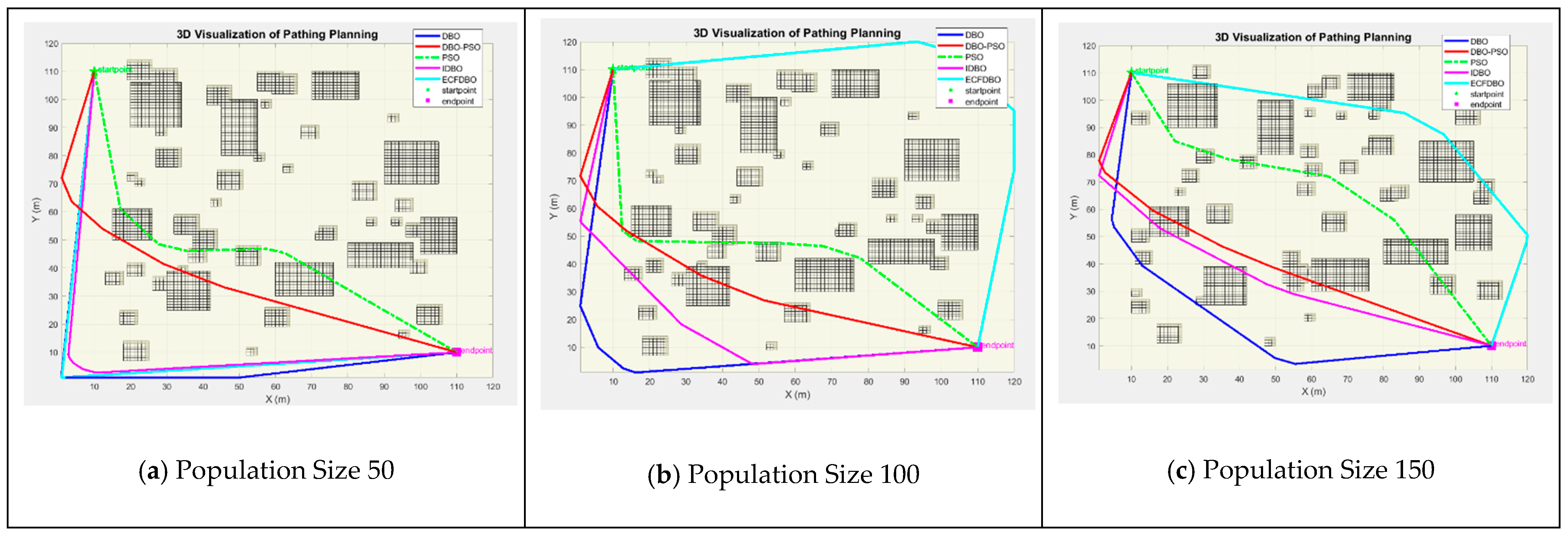
The results of the experiments are presented in

Table 7. Comparative experimental data of five algorithms.

Population Size	Algorithm	Total Path Cost	Path Length Cost	Smoothness Cost	Flight Altitude Cost	Average Computation Time
50	DBO-PSO	284.91	182.11	32.29	70.51	0.84
	DBO	510.41	219.48	61.71	229.22	1.01
	PSO	344.67	172.93	78.82	92.93	0.63
	IDBO	312.83	220.06	31.77	61.01	1.06
	ECFDBO	518.78	218.97	64.82	235.00	13.16
100	DBO-PSO	289.00	183.99	36.09	68.92	1.35
	DBO	480.12	209.74	35.38	235.00	1.92
	PSO	372.16	180.4	76.44	115.28	1.06
	IDBO	304.64	202.27	40.78	61.59	1.81
	ECFDBO	363.54	222.37	57.01	84.17	16.73
150	DBO-PSO	283.11	160.43	35.14	87.54	1.84
	DBO	302.72	178.57	40.11	64.17	2.24
	PSO	299.71	165.60	41.20	92.91	1.43
	IDBO	288.28	181.13	33.63	73.52	1.89
	ECFDBO	296.30	190.99	41.96	63.35	21.00

. In Figure 7, Figure 8 and Figure 9, panels (a), (b) and (c) correspond to population sizes of 50, 100, and 150.

In the aforementioned experimental results, Table 7 presents a comparison of the total path cost, path length, smoothness cost, flight altitude cost, and average computation time among the five algorithms under different population sizes; Figure 7 shows the convergence comparison of the five algorithms under different population sizes. Figure 8 displays the three-dimensional path diagrams of the five algorithms under different population sizes. Figure 9 provides the top-view path diagrams of the five algorithms under different population sizes.

4.3. Experimental Results Analysis

The total path cost is a primary metric for assessing the quality of path planning solutions, comprehensively reflecting multiple factors such as the path length, smoothness, and altitude constraints. As shown in Table 7, across different population sizes, the total path cost of DBO-PSO is consistently lower than that of DBO, PSO, IDBO, and ECFDBO. When the population size is 50, the total path cost of DBO-PSO is 284.91, which is 44.2%, 17.3%, 8.9%, and 45.1% lower than that of DBO at 510.41, PSO at 344.67, IDBO at 312.83, and ECFDBO at 518.78, respectively. When the population size is 100, DBO-PSO achieves 289.00, which is 39.8%, 22.3%, 5.1%, and 20.5% lower than that of DBO at 480.12, PSO at 372.16, IDBO at 304.64, and ECFDBO at 363.54, respectively. At population size 150, DBO-PSO attains 283.11, which is 6.5%, 5.5%, 1.8%, and 4.5% lower than that of DBO at 302.72, PSO at 299.71, IDBO at 288.28, and ECFDBO at 296.30, respectively. These results demonstrate that DBO-PSO possesses stronger global exploration capability and can more rapidly approach high-quality solution regions. DBO-PSO maintains a consistent advantage across all population sizes, highlighting the inherent efficiency and stability of its algorithmic structure. The performance improvement is not solely reliant on an increase in population size.

Path length cost is a primary metric for evaluating the performance of UAV path planning algorithms, as it directly determines the mission execution time, energy consumption, and overall operational efficiency. Shorter paths correspond to a higher mission response efficiency, a factor that is essential for the economic viability and practical utility of UAVs. As shown in Table 7, when the population size is 50, the path length of DBO-PSO is 182.11, which is 17.0%, 17.2%, and 16.9% lower than that of DBO at 219.48, IDBO at 220.06, and ECFDBO at 218.97, respectively. When the population size is 100, DBO-PSO achieves 183.99, which is 12.3%, 9.0%, and 17.3% lower than that of DBO at 209.74, IDBO at 202.27, and ECFDBO at 222.37, respectively. At population size 150, DBO-PSO attains 160.43, which is 10.2%, 3.1%, 11.4%, and 16.0% lower than that of DBO at 178.57, PSO at 165.60, IDBO at 181.13, and ECFDBO at 190.99, respectively. These results demonstrate that DBO-PSO exhibits strong capability in seeking global optimal solutions, particularly at larger population sizes where it achieves the shortest path among all algorithms. By incorporating PSO’s global memory and information-sharing mechanism, each individual in DBO-PSO relies on its own experience while being guided by the historically best positions discovered by the entire population. This mechanism enables superior path segments to propagate rapidly within the population, effectively concentrating search efforts on more promising solution regions. The DBO-PSO algorithm is capable of planning shorter paths, thereby validating the effectiveness of its improvement strategies and providing robust algorithmic support for improving operational efficiency and reducing operational costs in practical UAV applications.

Path smoothness cost is directly related to the safety and stability of UAV flight. A path with a higher smoothness cost typically contains numerous sharp turns and acute angles, which can force the UAV to frequently decelerate and adjust its altitude, significantly increasing the burden on the control system and prolonging mission duration. As shown in Table 7, DBO-PSO consistently achieves lower smoothness costs than DBO, PSO, and ECFDBO across all population sizes. For instance, at population size 50, the smoothness cost of DBO-PSO is 32.29, which is 47.7%, 59.0%, and 50.2% lower than that of DBO, PSO, and ECFDBO, respectively. At population size 150, DBO-PSO achieves 35.14, outperforming DBO, PSO, and ECFDBO by 12.4%, 14.7%, and 16.3%, respectively. Although IDBO achieves slightly better results in some cases, DBO-PSO remains highly competitive. The significant improvement in path smoothness indicates that the paths planned by DBO-PSO effectively reduce the control difficulty for UAVs, enabling smoother turns and altitude adjustments. As visualized in Figure 8 and Figure 9, the paths generated by DBO-PSO exhibit smooth and natural curved shapes, while those generated by DBO and PSO contain sharper turns, making DBO-PSO more suitable for application in complex three-dimensional environments.

Flight altitude cost directly reflects the algorithm’s ability to keep the UAV within a predefined safe altitude range. Excessively low altitudes increase collision risks with terrain, while excessively high altitudes may cause signal loss or unnecessary energy consumption. As shown in Table 7, DBO-PSO consistently achieves lower flight altitude costs than DBO, PSO, and ECFDBO across most population sizes. For instance, at population size 50, the altitude cost of DBO-PSO is 70.51, which is 69.2%, 24.1%, and 70.0% lower than that of DBO, PSO, and ECFDBO, respectively. At population size 100, DBO-PSO achieves 68.92, outperforming DBO, PSO, and ECFDBO by 70.7%, 40.2%, and 18.1%, respectively. These results confirm that the proposed algorithm, through Kent chaotic mapping and the PSO velocity–position update mechanism, can effectively guide the UAV to fly within the desired altitude range while balancing other objectives.

Average computation time reflects the computational efficiency of each algorithm. As shown in Table 7, the computation time of DBO-PSO increases from 0.84 s at population size 50 to 1.35 s at size 100 and 1.84 s at size 150, which is expected as more individuals require evaluation. Compared to the other algorithms, DBO-PSO consistently achieves a lower computation time than DBO, IDBO, and ECFDBO across all population sizes. Although PSO achieves slightly faster computation times, DBO-PSO remains highly competitive. The computational advantage over DBO and its variants is attributed to the incorporation of the PSO velocity–position update mechanism, which provides more efficient global search guidance and reduces unnecessary random explorations, thereby accelerating the convergence process without sacrificing solution quality.

4.4. Ablation Study

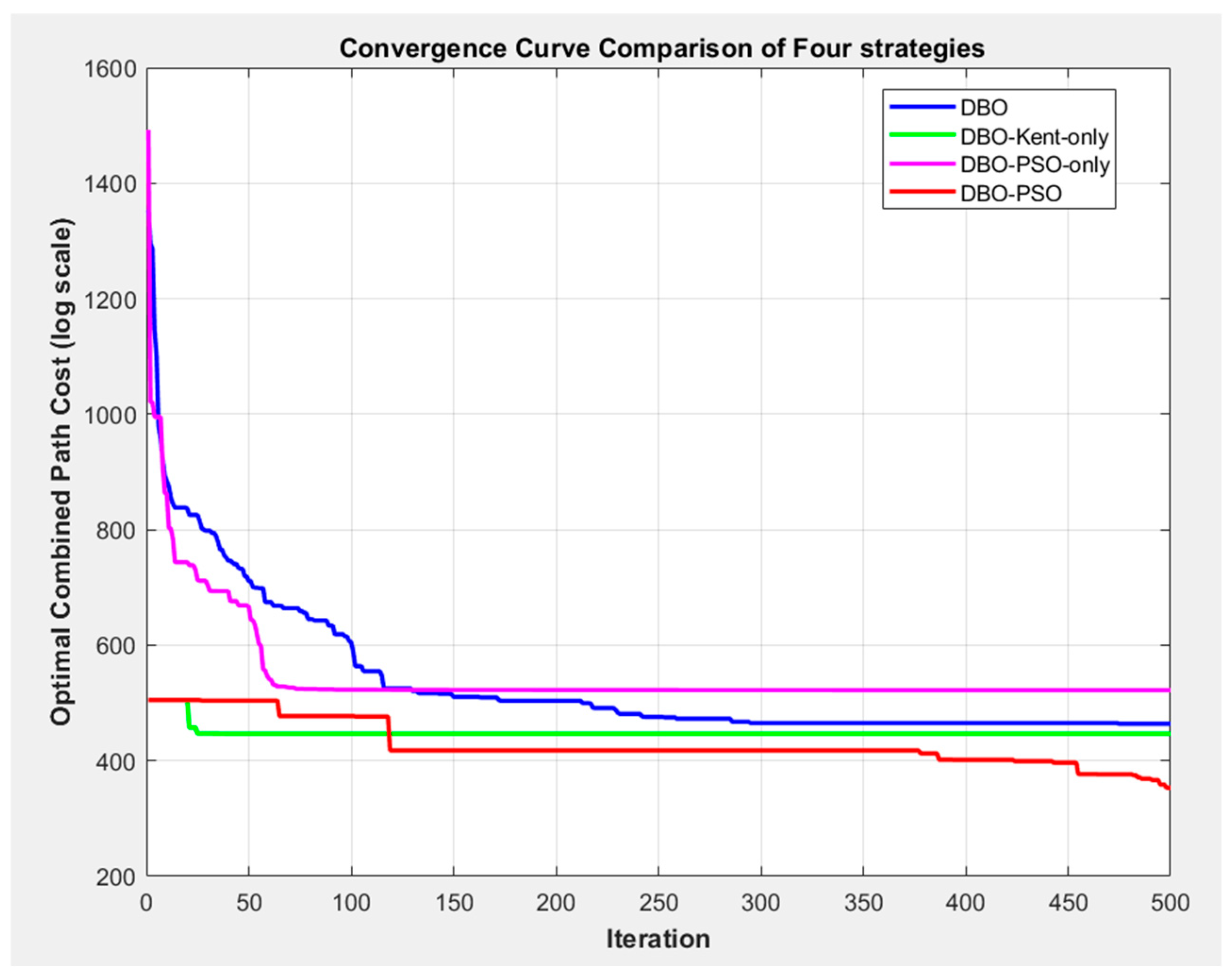
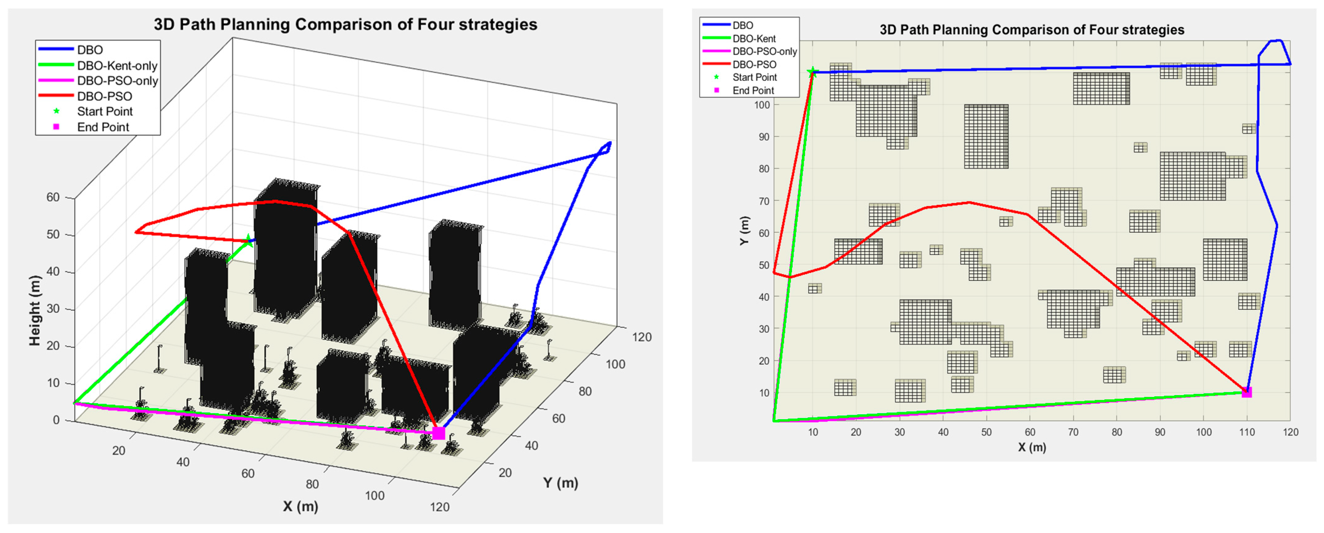
To systematically evaluate the contribution of each improvement component in the proposed DBO-PSO scheme, we conducted ablation experiments under identical environmental conditions, parameter settings, and software frameworks. Specifically, we selected the unimproved DBO strategy (DBO), the DBO strategy adopting the Kent chaotic map initialization (DBO–Kent-only), and the DBO strategy using the PSO-based velocity–position update strategy (DBO-PSO-only). A total of four schemes were compared: DBO, DBO–Kent-only, DBO-PSO-only, and the complete DBO-PSO scheme proposed in this paper. For the urban path planning scenario, thirty independent experiments were performed for each scheme, and one representative result was selected for visualization analysis. The fitness curves are shown in Figure 10, the 3D path planning comparisons of the four strategies are shown in Figure 11, and the ablation study results are summarized in

Table 8. Ablation study statistical results.

Algorithm	Min	Max	Mean	Variance	Avg Distance	Avg Smoothness
DBO	275.5231	675.9274	446.1461	16,635.0910	233.17	36.06
DBO–Kent-only	265.0455	446.7831	368.1375	2325.1700	223.29	27.18
DBO-PSO-only	214.9891	522.0387	349.7600	5824.4536	214.64	25.69
DBO-PSO	201.0758	399.5370	341.6121	1048.3579	209.41	30.14

and

Table 9. Last experiment detailed results comparison.

Algorithm	Combined Cost	Path Length	Smoothness Cost
DBO	463.9275	246.72	37.22
DBO–Kent-only	446.7831	218.97	34.23
DBO-PSO-only	422.0387	219.02	35.17
DBO-PSO	353.0370	216.05	30.14

.

The ablation study results clearly demonstrate the contribution of each improvement component. As shown in the statistical tables, the original DBO yields the highest total path cost at 463.93 and the longest path length at 246.72 m, with a smoothness cost of 37.22. Introducing only the Kent chaotic map reduces the integrated cost to 446.78, shortens the path length to 218.97 m, and lowers the smoothness cost to 34.23, indicating that a more uniformly distributed initial population effectively improves the solution quality. Using only the PSO velocity–position update mechanism also reduces the integrated cost to 422.04. The complete DBO-PSO, combining both strategies, achieves the best overall performance, with the lowest integrated cost at 353.04, the shortest path length at 216.05 m, and the smallest smoothness cost at 30.14. These results confirm that both the Kent chaotic map and the PSO velocity–position update mechanism positively contribute to the algorithm’s performance, and their integration yields complementary benefits.

4.5. DBO-PSO Algorithm Complexity Analysis

A comprehensive understanding and evaluation of an algorithm necessitates an analysis of its computational complexity, as this directly impacts algorithmic efficiency. Key parameters including population size (n), variable dimensionality (d), and maximum iteration number (T) exert a remarkable impact on computational complexity. In consideration of the above factors, the overall computational complexity of the DBO-PSO algorithm can be quantitatively analyzed.

$$\begin{array}{ll}O\left(DBO-PSO\right)& =O\left(Problem Definition\right)+O\left(Population Initialization\right)+O\left(Fitness Assessment\right)\\ & +O\left(Rolling Ball Behavior Update\right)+O\left(Reproductive Behavior Update\right)\\ & +O\left(Foraging Behavior Update\right)+O\left(Theft Incident Update\right)\\ & +O\left(Optimal Solution Update\right)\\ & =O\left(n·d\right)+O\left(n·d\right)+O\left(n·f\right)+T·\left[O\left(n\right)+O\left(n·\left(d+f\right)\right)+O\left(n\right)\right]=O\left(T·n·\left(d+f\right)\right)\end{array}$$

To thoroughly analyze the computational complexity of DBO-PSO, a comparison is made with some commonly used algorithms such as PSO, HHO, and ABC. The complexities of PSO, ABC, and HHO are expressed as $O(T\times n\times d)$, suggesting that these algorithms typically include setting up the initial population, calculating the fitness values, and updating positions. In contrast, the complexity of DBO-PSO is expressed as $O(T\times n\times (d+f\left)\right)$. This implies that DBO-PSO possesses the characteristic of being sensitive to the fitness function, and its actual performance is significantly influenced by the complexity $O\left(f\right)$ of the fitness function. This complexity analysis demonstrates that DBO-PSO retains the advantages of bio-inspired algorithms while maintaining computational efficiency comparable to that of classical optimization algorithms, making it particularly suitable for large-scale engineering optimization problems where complex sorting operations are not required.

5. Discussion

A hybrid algorithm termed DBO-PSO is proposed by integrating Kent chaotic mapping and the PSO velocity–position update mechanism into the dung beetle optimizer for UAV 3D path planning. The proposed algorithm achieves a 44.2% reduction in total path cost compared to standard DBO at a population size of 50, and ranks second among nine algorithms on the CEC2022 benchmark suite.

The observed performance improvements can be attributed to two complementary mechanisms. Firstly, the Kent chaotic map generates a more uniformly distributed initial population than the random initialization used in standard DBO. This enhances population diversity from the beginning of the search process, reducing the likelihood of premature convergence to suboptimal solutions. Secondly, the incorporation of the PSO velocity–position update introduces an individual memory and global best guidance mechanism that is largely absent in the original DBO. While DBO relies on role-specific stochastic updates, DBO-PSO enables each beetle to retain its own historical best position and share information with the entire population. This accelerates the propagation of promising path segments and improves the balance between global exploration and local exploitation, particularly in the multimodal and hybrid benchmark functions of the CEC2022 suite.

Consistent with previous studies on DBO variants, hybrid strategies generally improve algorithmic performance. However, unlike IDBO, which emphasizes local refinement through spiral search around the current best solution, DBO-PSO focuses on global exploration via the memory and information-sharing mechanism of PSO. This distinction explains why DBO-PSO achieves better performance on multimodal functions where escaping local optima is critical, while IDBO performs slightly better on certain unimodal functions. Compared to ECFDBO, which employs a dynamic force-field mutation strategy, DBO-PSO achieves a substantially lower total path cost and significantly shorter computation time in path planning experiments, indicating that the PSO-based mechanism is computationally more efficient for the tested scenario.

From a theoretical perspective, this study demonstrates that hybridizing the role-based exploration mechanism of DBO with the memory-guided convergence of PSO can effectively balance global search and local exploitation. The computational complexity analysis confirms that DBO-PSO maintains efficiency comparable to classical swarm intelligence algorithms, providing a reference for future hybrid algorithm designs. From a practical standpoint, DBO-PSO offers a viable solution for pre-flight UAV trajectory planning in static urban environments. The ability to generate shorter, smoother, and altitude-compliant paths can reduce energy consumption, improve flight safety, and lower operational costs for applications such as urban logistics, disaster assessment, and infrastructure inspection.

Nevertheless, the experimental environment remains a simplified representation of real three-dimensional scenarios. Dynamic obstacles, weather disturbances, and real-time replanning requirements were not considered. Meanwhile, the three-dimensional UAV path model retains potential for further improvement and optimization, in which different weighting priorities should be adopted to align with real-world application scenarios for different practical applications.

6. Conclusions

This paper proposed a hybrid algorithm named DBO-PSO for UAV path planning in three-dimensional urban environments. The method introduced Kent chaotic mapping for population initialization and incorporated the velocity–position update mechanism from particle swarm optimization into the dung beetle optimizer to enhance the global search capability. The quantitative results demonstrated clear advantages of the proposed algorithm. Benchmark tests on the CEC2022 suite showed that DBO-PSO had a competitive performance across all benchmark functions, and ranked second among nine algorithms in the Friedman test, indicating competitive performance in convergence accuracy and robustness.

In three-dimensional path planning experiments, compared with DBO, PSO, IDBO, and ECFDBO at population size 50, DBO-PSO reduced the total path cost by 44.2%, 17.3%, 8.9%, and 45.1%, respectively. The ablation study results clearly demonstrate the contribution of each improvement component. In conclusion, the proposed algorithm demonstrates competitive performance in balancing multiple objectives including path length, smoothness, and altitude constraints, while maintaining favorable computational efficiency.

7. Limitations

Despite the promising results achieved by the proposed DBO-PSO algorithm in UAV path planning, several limitations of the current study should be acknowledged.

The synthetic 3D urban environment is oversimplified relative to real-world scenarios. The experimental validation is conducted on a procedurally generated environment comprising idealized cuboid buildings and conical trees implemented in MATLAB. This setup does not fully capture the complexity of real urban airspace, which involves irregular obstacle geometries such as overhanging structures and curved facades, dynamic no-fly zones including airports, government facilities, and privacy-sensitive areas, meteorological disturbances like sudden wind gusts, precipitation, and turbulence, as well as variable low-altitude air traffic density from other UAVs or manned aircraft. Furthermore, the paper does not specify how a real terrain map would be obtained or processed. The binary obstacle mask and uniform height matrix employed also fail to capture the geometric complexity of real structures, such as overhanging building features, curved facades, or transparent surfaces.

Another limitation of the current investigation is that it is designed for pre-flight planning and does not support real-time trajectory replanning. Specifically, the algorithm generates a static trajectory based on known environmental information before the UAV commences its mission. It does not yet account for in-flight adjustments in response to external changes, such as newly detected dynamic obstacles including birds, other UAVs, or construction cranes, or sudden weather deterioration such as changes in wind speed or direction. Consequently, the current framework lacks the capability for online trajectory recalculation, which is essential for robust operation in dynamic urban environments.

A further limitation is that the adaptation to real UAV hardware constraints and multi-UAV cooperative scenarios has not been addressed. The paper does not specify which UAV attributes are considered, for instance, maximum turn angle, climb and descent rate, velocity limits, or sensor accuracy. The computational efficiency of DBO-PSO, while analyzed in terms of complexity, has not been validated on embedded flight control hardware with limited processing power and memory. Real-time constraints such as path generation within one second for dynamic replanning remain unexplored. Additionally, the extension to multi-UAV cooperative operations has not been investigated, despite its relevance to real scenarios where fleets of UAVs often operate simultaneously. Such an extension would introduce further constraints including inter-UAV collision avoidance, communication connectivity, task allocation, and coordination under limited airspace capacity.

References

1. Du, P.F.; Shi, Y.Q.; Cao, H.T.; Garg, S.; Alrashoud, M.; Shukla, P.K. AI-enabled trajectory optimization of logistics UAVs with wind imparts in smart cities. IEEE Trans. Consum. Electron. 2024, 70, 3885–3897. [Google Scholar] [CrossRef]
2. Zhao, X.; Wang, X.; Dai, Y.; Qiu, Q. Joint optimization of loading, mission abort and rescue site selection policies for UAV. Reliab. Eng. Syst. Saf. 2024, 244, 109955. [Google Scholar] [CrossRef]
3. Pádua, L.; Marques, P.; Dinis, L.-T.; Moutinho-Pereira, J.; Sousa, J.J.; Morais, R.; Peres, E. Detection of leak aeras in vineyard irrigation systems using UAV-based data. Drones 2024, 8, 187. [Google Scholar] [CrossRef]
4. Liu, X.; Zhong, W.; Wang, X.; Duan, H.; Fan, Z.; Jin, H.; Huang, Y.; Lin, Z. Deep reinforcement learning-based 3D trajectory planning for cellular connected UAV. Drones 2024, 8, 199. [Google Scholar] [CrossRef]
5. Peña-Delgado, A.F.; Peraza-Vázquez, H.; Almazán-Covarrubias, J.H.; Cruz, N.T.; García-Vite, P.M.; Morales-Cepeda, A.B.; Ramirez-Arredondo, J.M. A Novel Bio-Inspired Algorithm Applied to Selective Harmonic Elimination in a Three-Phase Eleven-Level Inverter. Math. Probl. Eng. 2020, 8856040. [Google Scholar] [CrossRef]
6. Sun, J.; Tang, J.; Lao, S. Collison avoidance for cooperative UAVs with optimized artificial potential field algorithm. IEEE Access 2017, 5, 18382–18390. [Google Scholar] [CrossRef]
7. Mishmast Nehi, H.; Ashayerinasab, H.A.; Allahdadi, M. Solving methods for interval linear programming problem: A review and an improved method. Oper. Res. 2018, 20, 1205–1229. [Google Scholar] [CrossRef]
8. Shang, E.; Dai, B.; Nie, Y.M.; Zhu, Q.; Xiao, L.; Zhao, D. An improved A-star based path planning algorithm for autonomous land vehicles. Int. J. Adv. Robot. Syst. 2020, 17, 591–617. [Google Scholar] [CrossRef]
9. Li, X.M.; Lu, Y.; Zhao, X.Y.; Deng, X.; Xie, Z. Path planning for intelligent vehicles based on improved D* lite. J. Supercomput. 2024, 80, 1294–1330. [Google Scholar] [CrossRef]
10. Langari, S.M.; Vahdatikhaki, F.; Hammad, A. Improving the performance of RRT path planning of excavators by embedding heuristic rules. Adv. Eng. Inform. 2024, 62, 102724. [Google Scholar] [CrossRef]
11. Li, Y.J.; Wei, W.; Gao, Y.; Wang, D.; Fan, Z. PQ-RRT*: An improved path planning algorithm for mobile robots. Expert Syst. Appl. 2020, 152, 113425. [Google Scholar] [CrossRef]
12. Xie, R.L.; Meng, Z.J.; Want, L.F.; Li, H.; Wang, K.; Wu, Z. Unmanned Aerial Vehicle Path Planning Algorithm Based on Deep Reinforcement Learning in Large-Scale and Dynamic Environments. IEEE Access 2021, 9, 24884–24900. [Google Scholar] [CrossRef]
13. Huang, X.; Zhang, Z.J.; Sun, P.; Tang, Y.D.; Liu, Y.P. A survey of path planning algorithms based on deep reinforcement learning. Robot 2026, 48, 196–216. (In Chinese) [Google Scholar]
14. Zhang, M.T.; Zhang, J.; He, C.F. Review of metaheuristic algorithms research. Comput. Eng. Appl. 2026, 62, 40–53. (In Chinese) [Google Scholar]
15. Goldberg, D.E. Genetic Algorithms in Search, Optimization, and Machine Learning; Addison-Wesley Publishing Company, Inc.: Boston, MA, USA, 1989. [Google Scholar]
16. Harada, T.; Alba, E. Parallel genetic algorithms: A useful survey. ACM Comput. Surv. 2021, 53, 1–39. [Google Scholar] [CrossRef]
17. Opara, K.R.; Arabas, J. Differential evolution: A survey of theoretical analyses. Swarm Evol. Comput. 2019, 44, 546–558. [Google Scholar] [CrossRef]
18. Abbasi, B.; Majidnezhad, V.; Mirjalili, S. ADE: Advanced differential evolution. Neural Comput. Appl. 2024, 36, 15407–15438. [Google Scholar] [CrossRef]
19. Kirkpatrick, S.; Gelatt, C.; Vecchi, M. Optimization by simulated annealing. Science 1983, 220, 671–680. [Google Scholar] [CrossRef]
20. Chauhan, D.; Yadav, A. A comprehensive survey on artificial electric field algorithm: Theories and applications. Arch. Comput. Methods Eng. 2024, 31, 2663–2715. [Google Scholar] [CrossRef]
21. Mirjalili, S. SCA: A sine cosine algorithm for solving optimization problems. Knowl.-Based Syst. 2016, 96, 120–133. [Google Scholar] [CrossRef]
22. Abualigah, L.; Diabat, A.; Mirjalili, S.; Elaziz, M.A.; Gandomi, A.H. The arithmetic optimization algorithm. Comput. Methods Appl. Mech. Eng. 2021, 376, 113609. [Google Scholar] [CrossRef]
23. Rai, R.; Das, A.; Ray, S.; Dhal, K.G. Human-inspired optimization algorithms: Theoretical foundations, algorithms, open research issues and application for multi-level thresholding. Arch. Comput. Methods Eng. 2022, 28, 2513–5352. [Google Scholar] [CrossRef]
24. Kennedy, J.; Eberhart, R. Particle swarm optimization. In Proceedings of the IEEE International Conference on Neural Networks, Perth, Australia, 27 November–1 December 1995; IEEE: New York, NY, USA, 1995; pp. 1942–1948. [Google Scholar]
25. Yang, Y.; Sun, L.; Fu, Y.; Feng, W.; Xu, K. Three-dimensional UAV trajectory planning based on improved sparrow search algorithm. Symmetry 2025, 17, 2071. [Google Scholar] [CrossRef]
26. Blum, C. Ant colony optimization: A bibliometric review. Phys. Life Rev. 2024, 51, 87–95. [Google Scholar] [CrossRef] [PubMed]
27. Yang, J.; Yan, F.; Zhang, J.; Peng, C. Hybrid chaos game and grey wolf optimization algorithms for UAV path planning. Appl. Math. Model. 2025, 142, 115979. [Google Scholar] [CrossRef]
28. Yang, Y.; Fu, Y.J.; Lu, D.Y.; Xiang, H.; Xu, K. Three-dimensional unmanned aerial vehicle trajectory planning based on the improved whale optimization algorithm. Symmetry 2024, 16, 1561. [Google Scholar] [CrossRef]
29. Yang, Y.; Fu, Y.J.; Li, D.L.; Xu, K.J. Multi-UAVs Trajectory Planning Based on Starfish Optimization Algorithm. Sci. Technol. Eng. 2026, 26, 387–394. [Google Scholar]
30. Xue, J.K.; Shen, B. Dung Beetle Optimizer: A New Meta-Heuristic Algorithm for Global Optimization. J. Supercomput. 2022, 79, 7305–7336. [Google Scholar] [CrossRef]
31. Shen, Q.W.; Zhang, D.M.; Xie, M.S.; He, Q. Multi-strategy enhanced dung beetle optimizer and its application in three-dimensional UAV path panning. Symmetry 2023, 15, 1432. [Google Scholar] [CrossRef]
32. Zheng, X.; Liu, R.; Li, S. A Novel Improved Dung Beetle Optimization Algorithm for Collaborative 3D Path Planning of UAVs. Biomimetics 2025, 10, 420. [Google Scholar] [CrossRef]
33. Li, X.L.; Jiang, H.; Yang, F. Improved dung beetle optimizer algorithm with multi-strategy for global optimization and UAV 3D path planning. IEEE Access 2024, 12, 69240–69257. [Google Scholar] [CrossRef]
34. Zhang, R.; Chen, X.; Li, M. Multi-UAV Cooperative Task Assignment Based on Multi-Strategy Improved DBO. Clust. Comput. 2025, 28, 195. [Google Scholar] [CrossRef]
35. Liu, K.; Dai, Y.; Liu, H. Improvement of Dung Beetle Optimization Algorithm Application to Robot Path Planning. Appl. Sci. 2025, 15, 396. [Google Scholar] [CrossRef]
36. Chen, Q.; Wang, Y.J.; Sun, Y.F. An improved dung beetle optimizer for UAV 3D path planning. J. Supercomput. 2024, 80, 26357–26567. [Google Scholar] [CrossRef]
37. Li, B.G.; Zhang, H.B.; Shi, X.P. A novel path planning for AUV based on Dung Beetle Optimisation Algorithm with deep Q-network. Int. J. Robot. Autom. 2025, 40, 65–73. [Google Scholar] [CrossRef]
38. Li, Z.H.; Luo, X.; Peng, Q.J.; Yang, Y. Cross-domain fault diagnosis using convolutional attention network with an improved dung beetle optimization algorithm. Meas. Sci. Technol. 2024, 36, 0161a5. [Google Scholar] [CrossRef]
39. Wang, H.Q.; Song, G.; Ge, C. 3D Path Planning of UAVs Based on Improved Dung Beetle Algorithm. Electron. Opt. Control 2024, 31, 55–61+82. (In Chinese) [Google Scholar]
40. Liu, J.J.; Shi, D.Y.; Wu, G.N. Hybrid chaotic optimization algorithm based on Kent map. Comput. Eng. Des. 2015, 36, 1498–1503. (In Chinese) [Google Scholar]
Figure 1. Schematic diagram of dung beetle population distribution.
Applsci 16 05243 g001
Figure 2. DBO algorithm flowchart.
Applsci 16 05243 g002
Figure 3. DBO-PSO algorithm flowchart.
Applsci 16 05243 g003
Figure 4. Average ranking chart of nine algorithms.
Applsci 16 05243 g004
Figure 5. Convergence curves comparison.
Applsci 16 05243 g005
Figure 6. Three-dimensional experimental city model.
Applsci 16 05243 g006
Figure 7. Comparison of convergence between five algorithms at different population sizes.
Applsci 16 05243 g007
Figure 8. Comparison of paths between five algorithms at different population sizes.
Applsci 16 05243 g008
Figure 9. Top-down comparison of paths between five algorithms at different population sizes.
Applsci 16 05243 g009
Figure 10. Convergence curves comparison of four strategies.
Applsci 16 05243 g010
Figure 11. 3D path planning comparison of four strategies.
Applsci 16 05243 g011