Active Distribution Network Voltage Control with a Physics-Informed Spatiotemporal Attention Network

Abstract

Active voltage control (AVC) in active distribution networks coordinates the reactive power outputs of distributed inverters to maintain bus voltages within secure limits. Although multi-agent reinforcement learning (MARL) shows promise for AVC, current methods face three main limitations: graph topologies rely on unweighted adjacency, ignoring physical parameters like line impedance and electrical distance; centralized critics output a single global Q-value, leading to coarse spatial credit assignment; and temporal critic modules suffer from vanishing gradients and representation drift. To address these issues, we propose physics-informed spatiotemporal multi-agent value learning (PST-MA), a physics-informed spatiotemporal value-learning framework integrating three coupled designs: a physics-informed graph attention mechanism with electrical-distance-aware sparsification; node-conditional value outputs utilizing a replicated-graph diagonal-extraction strategy; and a temporal latent compression module featuring a gated bypass and late action fusion. Experiments on the IEEE 33-bus and 141-bus systems validate the effectiveness of the proposed PST-MA method. Results demonstrate that it consistently achieves a higher controllable ratio than baseline methods for coordinated voltage regulation under uncertainty.

1. Introduction

Driven by the increasing penetration of renewable energy, distributed photovoltaic (PV) and wind resources are being widely deployed, transforming conventional one-way feeders into active distribution networks (ADNs) with bidirectional power flows [1,2,3,4]. Although this transition improves operational flexibility and sustainability, the intermittency and volatility of renewable generation introduce severe voltage quality challenges. Particularly during periods of low load and high generation, feeder-end voltages frequently exceed upper limits, threatening the stable operation of inverter-rich distribution grids [3,5,6,7]. Active voltage control (AVC) has therefore emerged as a key enabling technology for maintaining acceptable voltage profiles under high renewable penetration [2,8,9,10]. Unlike conventional voltage regulation schemes dominated by on-load tap changers and capacitor banks, AVC relies primarily on the fast and continuous reactive power regulation capabilities of distributed inverters, making it particularly suitable for minute-level voltage support [2,3,5].

Despite its practical importance, implementing effective AVC in real-world systems remains challenging. Firstly, controllable resources are geographically dispersed across the network; coordinating dozens or hundreds of inverter units creates a high-dimensional decision space. Secondly, reactive-power injections are strongly coupled through nonlinear alternating-current (AC) power-flow equations, meaning local adjustments can impact remote voltages and complicate global coordination [1,3]. More specifically, these couplings translate into two structural constraints on any AVC controller: a local box constraint ${\left({\mathrm{q}}_i^{\mathrm{PV}}\right)}^2\le {\left(s_{\mathrm{m}\mathrm{a}\mathrm{x},i}\right)}^2-{\left(p_i\right)}^2$ imposed by each inverter’s capability limit, and a global coupling that requires the joint reactive injections to keep every bus voltage within the safe band—a constraint that no individual inverter can satisfy in isolation. Thirdly, both renewable generation and load demand fluctuate rapidly and stochastically, requiring controllers to produce high-quality actions within short control intervals [4,5,8,9]. Given that centralized control approaches often suffer from prohibitive computational costs, communication overhead, and limited scalability, AVC in ADNs is naturally framed as a high-dimensional, strongly coupled, and non-stationary multi-agent coordination problem [2,6,8,11,12].

Existing AVC methods can be broadly divided into two categories. The first category consists of model-based optimization approaches, including sensitivity-based linearization and centralized optimal power flow (OPF) formulations [3,9]. These methods provide clear analytical structure, but they rely on accurate online state estimation and global measurements, and their computational and communication burdens can become a bottleneck when rapid response is required. The second category is data-driven control based on multi-agent reinforcement learning (MARL) [2,4,5,8,11]. MARL can directly learn distributed control policies through interaction with the environment and is therefore well suited to complex AVC settings. However, although the simulation environment still depends on offline topology and line parameters, existing methods do not yet exploit such physical information deeply enough during policy learning. Most graph-based approaches construct agent interaction graphs from simple communication or topological adjacency and do not explicitly encode line impedance or electrical distance [7,12,13,14]. As a result, the learned coordination pattern may fail to reflect the actual physical coupling of voltage responses. Moreover, under continuous-action centralized-training-and-decentralized-execution (CTDE), existing methods usually suffer from coarse spatial credit assignment [15,16,17,18,19]: the same magnitude of reactive-power adjustment can have very different local and global impacts depending on line impedance, bus location, and electrical distance; so, a single global value signal is often insufficient to characterize heterogeneous agent contributions. When complex temporal modules such as recurrent networks or Transformers are introduced, additional problems such as representation drift and value oscillation may arise during non-stationary multi-agent training [20,21,22,23].

To address these limitations, we propose PST-MA, a physics-informed spatiotemporal value-learning framework for AVC in active distribution networks. Under CTDE, PST-MA improves MARL value learning from three tightly coupled perspectives: physical topology awareness, temporal modeling, and spatial credit assignment. Specifically, line-parameter information is injected into graph attention to better model local electrical coupling; a learnable temporal compression design is introduced to exploit observation history without destabilizing training; and node-level value outputs are used to provide finer-grained credit signals for coordinated policy optimization. Systematic experiments on the Multi-Agent Power Distribution Network (MAPDN) benchmark [8] show that the proposed method yields more stable and more precise voltage regulation in complex distribution-network scenarios.

The main contributions can be summarized as follows:

• Existing multi-agent approaches primarily model interactions based on communication links or topological adjacency, which fails to capture the true electrical coupling governed by line parameters in distribution networks [10,12,13,14]. To overcome this limitation, we propose a graph-attention-based value modeling method that embeds physical priors within localized electrical neighborhoods. Specifically, key electrical quantities—such as line impedance and electrical distance—are explicitly incorporated into the attention mechanism, aligning the message-passing process within the value network more closely with actual power-flow coupling. Furthermore, imposing electrical-neighborhood constraints restricts the receptive field to local regions with pronounced physical coupling, enabling value modeling that is physically consistent and structurally interpretable at the graph level.
• We introduce a node-conditional value output and spatial credit-alignment mechanism. Instead of using a conventional centralized critic that produces a single global scalar value [15,24], the proposed critic directly decodes graph-node representations into individual agent-specific estimates. A gradient-isolation design ensures that each actor only receives the value gradient associated with its own node, enabling fine-grained spatial credit assignment within a shared critic [17,18,19,23].
• We design a spatiotemporally decoupled value-learning framework that balances critic-side temporal modeling with actor-side lightweight inference. On the critic side, historical observations are compressed into temporal latent variables through a learnable temporal module inspired by recent temporal latent attention [21,22]. A gated bypass alleviates cold-start instability, while delayed action fusion shortens the gradient path from the value function to the action and reduces gradient attenuation through the temporal encoder.
• We conduct systematic experiments on the MAPDN multi-agent distribution-network benchmark [8]. Across different network scales, the proposed method consistently outperforms representative baselines in voltage-control performance and training stability. Ablation studies further verify the complementarity of the three core components and clarify their individual contributions.

2. Related Work

2.1. Traditional Optimization and MARL for AVC

Research on active voltage control in distribution systems was initially dominated by model-based methods such as sensitivity analysis and optimal power flow. Agalgaonkar et al. investigated the impact of distributed PV on tap changers and autonomous regulators, proposing a coordinated strategy based on centralized OPF [3]. Although such methods feature well-defined mathematical structures and, in some cases, optimality guarantees, their dependence on accurate model parameters and the latency of centralized solution procedures limit their suitability for highly dynamic operating conditions.

In recent years, MARL has attracted increasing attention for AVC because it circumvents the need for an explicit online system model and inherently aligns with distributed control architectures [2,8]. Cao et al. were among the first to introduce multi-agent deep reinforcement learning for coordinated PV-inverter voltage regulation [2]. Wang et al. later proposed the MAPDN framework, formulating AVC as a decentralized partially observable Markov decision process (Dec-POMDP) and establishing an open-source benchmark environment for systematic comparison in this field [8]. More recently, Qu et al. incorporated explicit safety constraints into the MARL framework through primal-dual optimization and dual safety estimation [11], while Zhang et al. explored physics-informed MARL with graph knowledge for faster policy learning [14]. Recent application-oriented studies have further examined multi-timescale control, weak-grid operation, and flexible-network settings [4,5,6,9,10,25,26]. These studies have substantially advanced MARL-based AVC, but important limitations remain in interaction modeling, temporal reasoning, and credit assignment.

2.2. Physics-Informed Topology and Graph Representation Learning for AVC

Given the inherent graph structure of distribution networks, graph representation learning has emerged as an effective tool for encoding agent interactions in MARL-based voltage control [12,13,14,27,28]. Lee et al. introduced graph convolution into multi-agent AVC to aggregate neighboring-agent information for supporting control decisions [13]. Hu et al. proposed Multi-Agent Soft Actor-Critic with a Hierarchical Graph Recurrent Network (MASAC-HGRN), combining heterogeneous graph attention and gated recurrent unit (GRU)-based temporal modeling for decentralized voltage/reactive-power (Volt/VAR) control among heterogeneous agents [12].

Among existing graph-attention models, Graph Attention Network v2 (GATv2) is particularly well suited for this application. Brody et al. demonstrated that GATv2 achieves strictly dynamic attention by modifying the computation order of the original Graph Attention Network (GAT), thereby overcoming the query-independent ranking limitation of standard graph attention [29]. This property enables attention weights to flexibly adapt to pairwise feature differences, a highly desirable trait in power systems where coupling intensities vary across buses and feeders.

However, most existing graph-based AVC methods still construct interaction graphs based on communication neighborhoods or simple adjacency relations, failing to explicitly encode resistance, reactance, or electrical distance [7,12,13]. Even when physical priors are considered, their integration into the attention mechanism remains largely superficial [10,14,30]. In contrast, the proposed method embeds physical priors into GATv2 via both edge features and an additive bias channel. This mechanism is combined with k-nearest-neighbor(k-NN) sparsification to construct an electrically localized interaction topology that accurately reflects the underlying power-flow physics.

2.3. Temporal Modeling and Spatiotemporal Learning Under Partial Observability

Under the Dec-POMDP formulation, each agent receives only local observations of the environment; thus, leveraging observation history is critical for accurate value estimation [8]. Hausknecht and Stone proposed the Deep Recurrent Q-Network (DRQN) by integrating Long Short-Term Memory (LSTM) networks into the Deep Q-Network (DQN) architecture to address partial observability [20]. Building on this paradigm, recurrent architectures have been widely adopted in MARL. For instance, Hong et al. proposed the Deep Recurrent Policy Inference Q-Network (DRPIQN) for partially observable multi-agent settings [31], and QMIX implementations commonly employ DRQN-style agent networks [20,32]. While recurrent models effectively aggregate historical information, their sequential nature hinders parallelization and often falls short in capturing long-range dependencies.

Recently, Transformer-based temporal modeling has gained significant traction in both single-agent and multi-agent reinforcement learning. However, the memory footprint of the key-value (KV) cache in standard multi-head attention scales linearly with sequence length, presenting a bottleneck for real-time control under constrained computational resources. Deng and Woodland proposed Multi-head Temporal Latent Attention (MTLA), which compresses temporal key-value caches through hypernetwork-based fusion of neighboring steps and a stride-aware causal mask [21]. Transformer-based multi-agent communication (TMAC) further illustrates how Transformer-based communication and temporal feature extraction can improve partially observable multi-agent decision making [22]. These studies indicate that attention-based temporal modeling can improve long-horizon representation quality, but memory cost and training stability remain central concerns.

Crucially, temporal modeling alone is insufficient for structured environments. In many such systems, agents are highly coupled spatially, necessitating joint spatiotemporal representations. Power systems represent a quintessential example of this spatiotemporal coupling. Ngo et al. combined model-based estimation with a physics-informed graphical neural network to improve state estimation accuracy and physical consistency [33]. Su et al. further showed that physics-informed graph convolution can improve voltage prediction robustness in active distribution systems [30]. Related graph-attention control studies on grid emergency voltage regulation also confirm the value of coupling graph structure with temporal decision making [27]. Such studies underscore that joint spatiotemporal modeling yields more robust state representations in structured dynamical systems.

Motivated by these insights, our work focuses on spatiotemporal value modeling for MARL-based AVC. However, naively stacking temporal and graph modules can exacerbate training instability, as target-network updates may induce representation inconsistency [20,21,23]. PST-MA addresses this issue through a temporally compressed critic, a physics-informed graph-attention module, and a gated residual bypass that coordinates temporal and spatial information flow.

2.4. Credit Assignment and Node-Level Value Learning Under CTDE

In cooperative MARL, credit assignment—the process of allocating a global team reward to individual agent contributions—is widely recognized as a critical factor dictating learning efficiency and coordination quality [16,17]. Value decomposition constitutes a prominent class of methods to address this. Value-Decomposition Networks (VDNs) decompose the joint action-value function into a sum of local Q-values [34], while QMIX relaxes this additive assumption via a monotonic mixing network, preserving consistency between individual and joint greedy action selections [32]. Although these methods demonstrate strong performance in cooperative tasks, they are primarily designed for discrete action spaces, and the monotonicity constraint restricts their capacity to capture complex cooperation patterns [32,35]. QTRAN further relaxes both assumptions to encompass a broader class of factorizable value functions; however, its complex objective often renders practical optimization challenging [36].

Within the actor–critic framework, multi-agent deep deterministic policy gradient (MADDPG) adopts the centralized training with decentralized execution (CTDE) paradigm, training a global-information-conditioned centralized critic for each agent to mitigate environment non-stationarity, though it lacks an explicit structured credit decomposition [15]. The counterfactual multi-agent policy gradients method (COMA) improves credit assignment through a counterfactual baseline, although it is primarily tailored for discrete-action settings [37]. Yu et al. demonstrated the high efficacy of Proximal Policy Optimization (PPO) in cooperative multi-agent environments, a variant commonly referred to as multi-agent Proximal Policy Optimization (MAPPO) [24]. More recent CTDE analyses also emphasize that structured inference and observation treatment can materially affect multi-agent coordination quality [23]. However, such methods typically rely on a centralized value function and advantage estimation rather than explicit per-agent value decomposition.

Recently, graph-based value learning has emerged as a promising direction for fine-grained credit assignment. Li et al. proposed deconfounded value decomposition, which analyzes credit bias from a causal perspective and introduces a trajectory graph as a proxy confounder [38]. Chen and Tan measured predictive contribution to improve credit assignment in policy-gradient settings [17], while later studies explored asynchronous, counterfactual, and graph-interpretable mechanisms for disentangling heterogeneous agent contributions [18,19,39,40]. Nevertheless, in continuous-action actor–critic settings, systematic studies remain scarce regarding how to directly decode node-level graph representations into individual Q-values, and how to align these values with stable, agent-specific policy-gradient updates. The node-conditional value head and the replicate-graph diagonal-extraction mechanism proposed in this work are specifically designed to bridge this gap.

3. Problem Formulation

3.1. AVC Task Description

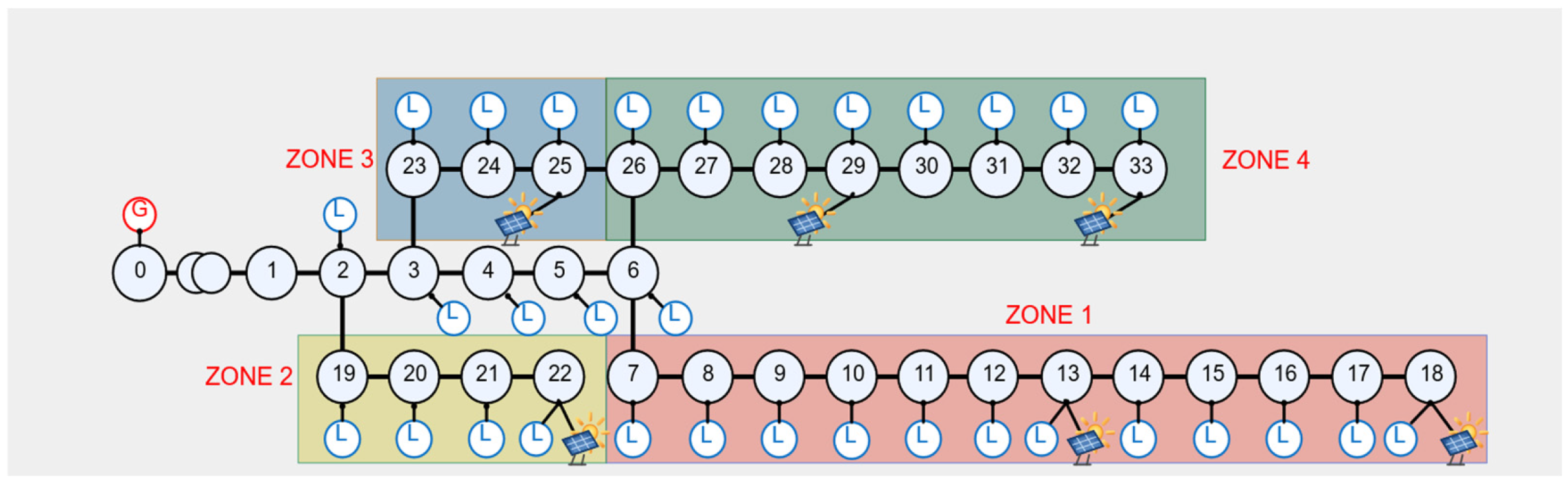
We investigate the active voltage control problem in a radial distribution network with $N_{\mathrm{bus}}$ buses and $N$ distributed PV inverters, as illustrated in Figure 1. Using the IEEE 33-bus feeder as an illustrative example, the system is partitioned into several electrical regions based on the shortest paths from the terminal buses to the main feeder. PV inverters within these regions operate as independent agents to achieve coordinated voltage regulation. At each control interval $\mathsf{\Delta }t$, each inverter adjusts its reactive-power output based on partial measurements from its own electrical region so that all bus voltages remain within a safe range $\left[\underset{\_}{v},\overline{v}\right]$—typically $\left[0.95,1.05\right]$ per unit (p.u.)—while minimizing reactive power consumption.

The physical topology of the distribution network is jointly defined by its line parameters and bus connectivity. Bus voltage magnitudes are implicitly constrained by the power flow equations, and the reactive power injection at any given node can impact remote bus voltages due to strong electrical coupling. Consequently, this strong coupling requires the multi-agent controllers to incorporate local topological information while coordinating to optimize system-level performance.

3.2. Physical Constraints and Control Objective

The steady-state operation of the network is governed by the AC power-flow equations. Let the voltage phasor at bus $k$ be $V_k=v_k{e}^{j{\theta }_k}$, where $v_k$ is the voltage magnitude and ${\theta }_k$ is the phase angle. The active- and reactive-power balance equations at bus $k$ are given by

$$P_k=v_k{\displaystyle \sum _{m=1}^{N_{\mathrm{bus}}}}{v}_m\left(G_{km}\mathrm{c}\mathrm{o}\mathrm{s}{\theta }_{km}+B_{km}\mathrm{s}\mathrm{i}\mathrm{n}{\theta }_{km}\right)$$

(1)

$$Q_k=v_k{\displaystyle \sum _{m=1}^{N_{\mathrm{bus}}}}{v}_m\left(G_{km}\mathrm{s}\mathrm{i}\mathrm{n}{\theta }_{km}-B_{km}\mathrm{c}\mathrm{o}\mathrm{s}{\theta }_{km}\right),$$

(2)

where $P_k$ and $Q_k$ denote the net active and reactive power injections at bus $k$, $G_{km}$ and $B_{km}$ are the real and imaginary parts of the bus-admittance matrix $Y$, ${\theta }_{km}$ = ${\theta }_k$ − ${\theta }_m$ is the voltage phase-angle difference between buses $k$ and $m$, and the index m runs over all buses electrically connected to bus $k$ through $Y$. Because each bus voltage is determined implicitly by these equations, a reactive-power injection at any single bus can propagate through $Y$ and influence voltage magnitudes across the entire network, giving rise to the strong nonlinear coupling that motivates coordinated multi-agent control.

The AVC objective is to minimize an operational cost while satisfying voltage-safety constraints. We write the optimization problem as

$$\underset{\left\{u_i\right\}}{\mathrm{m}\mathrm{i}\mathrm{n}}{\displaystyle \sum _{t=1}^T}\left[{\omega }_v\cdot {\displaystyle \frac{1}{N_{\mathrm{bus}}}}{\displaystyle \sum _{k=1}^{N_{\mathrm{bus}}}}\mathcal{B}\left(v_{k,t}\right)+{\omega }_q\cdot {\displaystyle \frac{1}{N}}{\displaystyle \sum _{i=1}^N}\left|q_{i,t}^{\mathrm{PV}}\right|\right]$$

(3)

$$\mathrm{s}.\mathrm{t}. \underset{\_}{v}\le v_{k,t}\le \overline{v}, \forall k\in \{1,\dots ,N_{\mathrm{bus}}\},\hspace{0.25em}\forall t,$$

(4)

$$\left|q_{i,t}^{\mathrm{PV}}\right|\le \sqrt{s_{\mathrm{m}\mathrm{a}\mathrm{x},i}^2-p_{i,t}^2}, \forall i\in \{1,\dots ,N\},\hspace{0.25em}\forall t,$$

(5)

where $\mathcal{B}\left(\cdot \right)$ is a voltage barrier function, ${\omega }_v$ and ${\omega }_q$ are the voltage-penalty and reactive-consumption weights, $s_{\mathrm{m}\mathrm{a}\mathrm{x},i}$ is the apparent-power capacity of inverter $i$, and $p_{i,t}$ is its active-power output. In this formulation, the barrier function penalizes expected voltage deviations, whereas the capacity constraint reflects the circular active–reactive capability limit of each inverter. Active power loss is treated as an independent economic evaluation metric rather than being directly included in the training objective. Here $T$ denotes the length of the control horizon (number of consecutive control intervals over which the cost is accumulated), and $u_i$ represents the joint sequence of normalized reactive-power control signals issued by all $N$ inverters across this horizon. The weights ${\omega }_v$ and ${\omega }_q$ are scalar coefficients shared across all buses rather than bus-specific. Under the cooperative Dec-POMDP formulation all inverter agents share a single team reward, and a uniform trade-off between voltage security and reactive-power consumption is sufficient to drive coordinated regulation; spatial selectivity is provided by the per-bus contribution of the barrier term $\mathcal{B}\left(·\right)$.

3.3. Dec-POMDP Formulation for AVC

The multi-inverter coordinated voltage-control problem is modeled as a decentralized partially observable Markov decision process (Dec-POMDP), denoted by $\mathcal{M}=⟨\mathcal{I},\mathcal{S},\left\{{\mathcal{O}}_i\right\},\left\{{\mathcal{A}}_i\right\},\mathcal{T},R,\gamma ⟩$.

Agent set $\mathcal{I}$: $\mathcal{I}=\{1,\dots ,\mathrm{N}\}$, where each agent controls one PV inverter.

Global state space $\mathcal{S}$: The global state concatenates all bus active and reactive injections, all PV active outputs, all inverter reactive set-points, and all complex bus voltages.

Local observation space ${\mathcal{O}}_{\mathrm{i}}$: Agent $\mathrm{i}$ receives local regional measurements,

$$o_{i,t}=\left\{\{P_k^{\mathrm{bus}},Q_k^{\mathrm{bus}}{\}}_{k\in {\mathcal{Z}}_i},\hspace{0.25em}{p}_{i,t}^{\mathrm{PV}},\hspace{0.25em}{q}_{i,t}^{\mathrm{PV}},\hspace{0.25em}\{\left|V_k\right|{\}}_{k\in {\mathcal{Z}}_i},\hspace{0.25em}\{{\theta }_k{\}}_{k\in {\mathcal{Z}}_i}\right\},$$

(6)

where ${\mathcal{V}}_{\mathrm{i}}$ is the bus set in the electrical region of agent $i$. If observation dimensions differ across regions, zero-padding is used to align them to a common dimension $d_o$. To mitigate partial observability, the environment stacks the most recent $H$ observations:

$${\tilde{o}}_{i,t}=\left[o_{i,t-H+1};\hspace{0.25em}{o}_{i,t-H+2};\hspace{0.25em}\dots ;\hspace{0.25em}{o}_{i,t}\right]\in {\mathbb{R}}^{H\cdot d_o}.$$

(7)

Missing history frames at the beginning of an episode are filled with zero vectors.

Joint action space $\mathrm{A}$:$\mathrm{A}={\displaystyle {\prod }_{\mathrm{i}=1}^{\mathrm{N}}}{\mathrm{A}}_{\mathrm{i}}$. The individual action ${\mathrm{a}}_{\mathrm{i},\mathrm{t}}\in \mathbb{R}$ is a normalized scalar reactive-power control signal. After reparameterized sampling and $\mathrm{t}\mathrm{a}\mathrm{n}\mathrm{h}$ squashing, the environment converts it into actual reactive injection:

$$q_{i,t}^{\mathrm{PV}}=u_{i,t}\cdot \sqrt{s_{\mathrm{m}\mathrm{a}\mathrm{x},i}^2-{\left(p_{i,t}^{\mathrm{PV}}\right)}^2},$$

(8)

where $u_{i,t}\in \left[-c_s,c_s\right]$ is the scaled control signal. This transformation guarantees that the action always satisfies the physical capability constraint $\left|q_{i,t}^{\mathrm{PV}}\right|\le \sqrt{s_{\mathrm{m}\mathrm{a}\mathrm{x},i}^2-{\left(p_{i,t}^{\mathrm{PV}}\right)}^2}$ and therefore decouples policy output from hard physical safety limits. The constant $c_s$ ∈ (0, 1] is a fixed scaling coefficient that bounds the magnitude of the normalized control signal and is set to 0.8 in our implementation, providing a small headroom against numerical chattering near the inverter capability boundary.

Transition function $\mathcal{T}$: The transition dynamics are implicitly defined by the AC power flow. Given the joint action, the environment updates inverter reactive injections and obtains the next state by solving the bus active- and reactive-power balance Equations (1) and (2) with a Newton–Raphson iterative solver, taking the substation bus as the slack bus. If the power flow fails to converge, the previous state is retained, an additional penalty is imposed, and the episode is terminated.

Reward function $\mathrm{R}$: All agents share the team reward

$$R\left(s_t,a_t\right)=-\left({\omega }_v\cdot {\displaystyle \frac{1}{N_{\mathrm{bus}}}}{\displaystyle \sum _{k=1}^{N_{\mathrm{bus}}}}\mathcal{B}\left(\left|V_{k,t}\right|\right)+{\omega }_q\cdot {\displaystyle \frac{1}{N}}{\displaystyle \sum _{i=1}^N}\left|q_{i,t}^{\mathrm{PV}}\right|\right).$$

(9)

The voltage barrier function takes the Bowl form:

$$\mathcal{B}\left(v\right)=\{\begin{array}{ll}-{\displaystyle \frac{c}{\sqrt{2\pi {\sigma }^2}}}\mathrm{e}\mathrm{x}\mathrm{p}\left(-{\displaystyle \frac{{\left(v-v_{\mathrm{ref}}\right)}^2}{2{\sigma }^2}}\right)+d,& \mathrm{if} \left|v-v_{\mathrm{ref}}\right|\le ϵ,\\ 2\left|v-v_{\mathrm{ref}}\right|-\eta ,& \mathrm{if} \left|v-v_{\mathrm{ref}}\right|>ϵ,\end{array}$$

(10)

Here $v$ denotes the voltage magnitude at a given bus and $v_{\mathrm{ref}}$ is the reference voltage (1.0 p.u.); $ϵ$ defines the half-width of the safe band around $v_{\mathrm{ref}}$; $\sigma$ controls the curvature of the inner Gaussian bowl and $c$ is its scaling coefficient; the constants d and $\eta$ are determined to ensure a smooth (continuously differentiable) transition at $\left|v-v_{\mathrm{ref}}\right|=$ $ϵ$.

Discount factor $\mathsf{\gamma }$: $\mathsf{\gamma }\in \left[\mathrm{0,1}\right)$. Under CTDE, each agent learns a parameterized policy ${\mu }_i:{\mathcal{O}}_i\to {\mathcal{A}}_i$ that maximizes the expected discounted return,

$$\underset{\{{\mu }_i{\}}_{i=1}^N}{\mathrm{m}\mathrm{a}\mathrm{x}}\hspace{0.25em}\mathbb{E}\left[{\displaystyle \sum _{t=0}^{\mathrm{\infty }}}{\gamma }^t{r}_t\right].$$

(11)

As the main safety metric, we use the controllable ratio (CR). At time step $t$, ${\mathrm{CR}}_t=1$ if and only if all bus voltages lie within the safe interval, and ${\mathrm{CR}}_t=0$ otherwise. The episode-level controllable ratio is defined as

$$\mathrm{CR}={\displaystyle \frac{1}{T}}{\displaystyle \sum _{t=1}^T}\mathbb{I}\left[\underset{\_}{v}\le \left|V_{k,t}\right|\le \overline{v},\hspace{0.25em}\forall k\right].$$

(12)

where $T$ is the total number of control steps within an evaluation episode.

In addition, the total active line loss $\mathrm{PL}=\sum _{\mathcal{l}\in {\mathcal{L}}_{\mathrm{line}}}{\mathrm{p}}_{\mathcal{l}}^{\mathrm{loss}}$ is reported as an economic indicator. Here ${\mathcal{L}}_{\mathrm{line}}$ is the set of all distribution lines and ${\mathrm{p}}_{\mathcal{l}}^{\mathrm{loss}}$ denotes the active power loss on line $\mathcal{l}$, both of which are obtained directly from the converged power-flow solution at every control step.

4. Our Method

4.1. Overall Architecture of the Proposed PST-MA

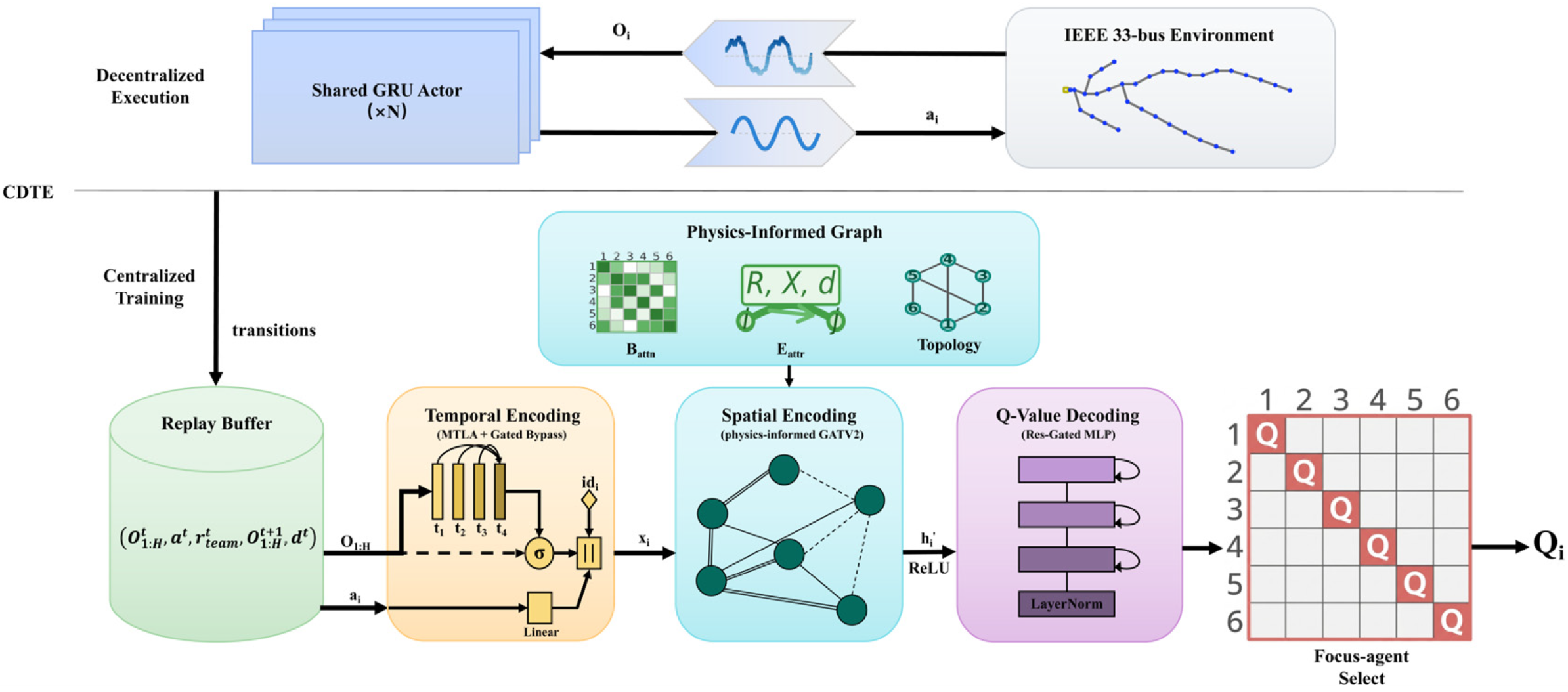
Existing multi-agent reinforcement learning (MARL) methods struggle to fully integrate spatiotemporal value learning with the physical coupling structure of distribution networks. Key limitations include the absence of explicit electrical priors in agent interaction graphs, the destabilizing impact of temporal modules on critic training, and the coarse credit assignment from centralized critics producing a single scalar output. To address these issues, we propose PST-MA. This approach introduces a centralized critic comprising three tightly coupled components: temporal compression, physics-informed graph attention, and node-conditional value decoding. The learning framework follows the centralized training with decentralized execution (CTDE) paradigm, employing an MADDPG-style actor–critic architecture. Within this framework, parameter-sharing actors generate continuous actions based on local observations, while a shared centralized critic processes global observations and joint actions to provide node-level value estimates for policy optimization.

The overall framework of PST-MA is shown in Figure 2. On the critic side, given the observation histories of all agents and their current actions, a temporal encoding module first performs learnable compression on each agent’s observation history to obtain a temporal summary representation. A gated bypass fusion mechanism is then used to adaptively combine the temporal summary with the projected current-frame observation. Subsequently, the current action is independently projected through a linear layer and directly injected into the spatial encoding stage, bypassing the temporal module via delayed action fusion. The resulting node features are then fed into a physics-informed graph attention layer, where message passing is carried out over the electrical coupling graph. Finally, a residual gated multilayer perceptron (MLP) decoder produces an individual Q-value for each agent node.

On the actor side, to avoid increasing policy-fitting difficulty with high-dimensional history inputs, only the most recent observation $o_{i,t}$ is used as the explicit input. A shared recurrent policy propagates the hidden state across time steps so that historical information is carried implicitly:

$$a_{i,t},\hspace{0.25em}{h}_{i,t}={\mu }_{\theta }\left(o_{i,t},h_{i,t-1}\right).$$

(13)

By contrast, the critic uses the full stacked observation history ${\tilde{o}}_{i,t}$, thus realizing an asymmetric design in which explicit temporal understanding is assigned to the critic and lightweight local inference is retained for the actor. This asymmetry preserves efficient execution while enabling the critic to provide more stable value estimates for policy learning.

4.2. Observation Encoding with Temporal Compression and Delayed Action Fusion

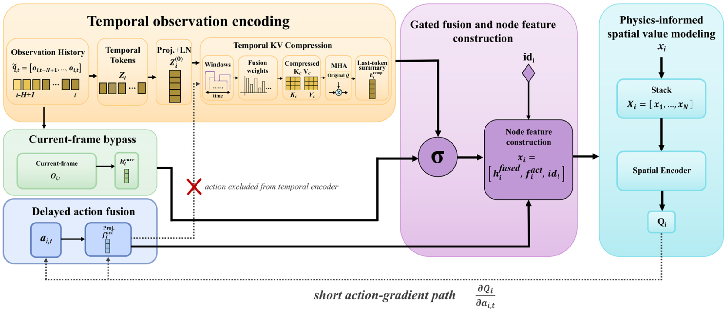
If the high-dimensional history vector ${\tilde{o}}_{i,t}\in {\mathbb{R}}^{H\cdot d_o}$, where $d_o$ denotes the padded per-frame observation dimension, is directly fed into the spatial graph encoder, both parameter count and training instability can increase substantially. More importantly, if the per-agent action $a_{i,t}$ is also routed through the temporal-attention module, the gradient $\partial Q/\partial a$ of the centralized critic value $\mathrm{Q}$ with respect to the joint continuous action vector a must traverse the entire temporal chain containing softmax operations, which exacerbates gradient attenuation. As shown in Figure 3, PST-MA therefore first compresses the observation history into a temporal latent variable, then injects reliable current-frame information through a gated bypass, and finally introduces the action only immediately before spatial reasoning.

For agent $i$, the stacked observation is reshaped into a temporal token sequence,

$$Z_i=\left[o_{i,t-H+1};\hspace{0.25em}{o}_{i,t-H+2};\hspace{0.25em}\dots ;\hspace{0.25em}{o}_{i,t}\right]\in {\mathbb{R}}^{H\times d_o},$$

(14)

which is projected into the embedding space through a linear layer and layer normalization:

$$Z_i^{\left(0\right)}=\mathrm{L}\mathrm{a}\mathrm{y}\mathrm{e}\mathrm{r}\mathrm{N}\mathrm{o}\mathrm{r}\mathrm{m}\left(W_{\mathrm{proj}}{Z}_i+b_{\mathrm{proj}}\right)\in {\mathbb{R}}^{H\times d_e}.$$

(15)

Here $W_{\mathrm{proj}}$ $\in {\mathbb{R}}^{(d_o\times d_e)}$ and $b_{\mathrm{proj}}$ $\in {\mathbb{R}}^{d_e}$ are the learnable projection weight and bias, $d_e$ is the per-token embedding dimension, and LayerNorm($\cdot$) denotes layer normalization applied along the feature axis. The embedded sequence is then processed by a lightweight temporal-compression module inspired by MTLA [21]. The key idea is to perform learnable temporal downsampling of the key–value sequence. The $H$ steps are partitioned into $G=\lceil H/s\rceil$ windows, and the key–value vectors within each window are fused with hypernetwork-generated weights:

$$K_c^{\left(g\right)}={\displaystyle \sum _{j=1}^s}{w}_j^{\left(g\right)}{K}_{(g-1)s+j}, V_c^{\left(g\right)}={\displaystyle \sum _{j=1}^s}{w}_j^{\left(g\right)}{V}_{(g-1)s+j},$$

(16)

where

$$w^{\left(g\right)}=\mathrm{s}\mathrm{o}\mathrm{f}\mathrm{t}\mathrm{m}\mathrm{a}\mathrm{x}\left(W_w\cdot \mathrm{m}\mathrm{e}\mathrm{a}\mathrm{n}\left(K_{(g-1)s+1:(g-1)s+s}\right)\right).$$

(17)

The compressed keys and values are then used together with the original query in multi-head attention,

$$\mathrm{A}\mathrm{t}\mathrm{t}\mathrm{n}\left(Q,K_c,V_c\right)=\mathrm{s}\mathrm{o}\mathrm{f}\mathrm{t}\mathrm{m}\mathrm{a}\mathrm{x}\left({\displaystyle \frac{Q{K}_c^{\mathrm{\top }}}{\sqrt{d_h}}}\right)V_c,$$

(18)

In the above, $s$ is the temporal downsampling stride (i.e., the window length), $G=\lceil H/s\rceil$ is the resulting number of windows, $K_{(g-1)s+j}$ and $V_{(g-1)s+j}$ are the per-step key and value vectors within window $g$, $w_j^{\left(g\right)}$ are the hypernetwork-generated fusion weights for window g, $W_w$ is the hypernetwork weight matrix, and $d_h$ is the per-head dimension used to scale the attention logits.

And the hidden state at the last time step is taken as the temporal summary,

$$h_i^{\mathrm{temp}}=\mathrm{M}\mathrm{T}\mathrm{L}\mathrm{A}\left(Z_i^{\left(0\right)}\right)\left[:,-1,:\right]\in {\mathbb{R}}^{d_e},$$

(19)

Relying on the temporal summary alone may expose the critic to cold-start noise early in training. To mitigate this effect, we introduce a gated bypass for the current observation. The current frame is first projected into the same latent dimension,

$$h_i^{\mathrm{curr}}=W_{\mathrm{bypass}}{o}_{i,t}+b_{\mathrm{bypass}},$$

(20)

Then a gate vector is adaptively computed from the concatenation of the temporal summary and current-frame projection,

$$g_i=\sigma \left(W_{\mathrm{gate}}\left[h_i^{\mathrm{temp}};h_i^{\mathrm{curr}}\right]+b_{\mathrm{gate}}\right),$$

(21)

And the fused representation is obtained by

$$h_i^{\mathrm{fused}}=g_i\odot h_i^{\mathrm{temp}}+\left(1-g_i\right)\odot h_i^{\mathrm{curr}}.$$

(22)

In Equations (20)–(22), $W_{\mathrm{bypass}}$ and $b_{\mathrm{bypass}}$ are the bypass projection parameters, $W_{\mathrm{gate}}$ and $b_{\mathrm{gate}}$ are the learnable gate parameters, [·;·] denotes vector concatenation along the feature axis, $\sigma$(·) is the element-wise sigmoid function, $\odot$ denotes element-wise (Hadamard) multiplication, and the gate vector $g_i$ $\in {\left(\mathrm{0,1}\right)}^{d_e}$ determines, on a per-feature basis, the convex mixing ratio between the temporal summary $h_i^{\mathrm{temp}}$ and the current-frame projection $h_i^{\mathrm{curr}}$. This design provides the spatial encoder with stable inputs early in training while still allowing richer temporal information to be exploited later.

To preserve a short gradient path from the value function to the action, PST-MA adopts delayed action fusion. The action is completely excluded from temporal compression and is projected only immediately before spatial encoding:

$$f_i^{\mathrm{act}}=W_{\mathrm{act}}{a}_{i,t}+b_{\mathrm{act}}.$$

(23)

The final node input to spatial value modeling is therefore

$$x_i=\left[h_i^{\mathrm{fused}};\hspace{0.25em}{f}_i^{\mathrm{act}};\hspace{0.25em}i{d}_i\right],$$

(24)

where $i{d}_i\in \{0,1{\}}^N$ is the one-hot identity of agent $i$, used to break node symmetry under parameter sharing. Through the combination of temporal compression, current-frame bypass, and delayed action fusion, critic-side temporal modeling is explicitly decoupled from actor-side policy-gradient propagation.

4.3. Physics-Informed Local Electrical Graph Construction and Spatial Attention Modeling

To ensure that graph attention reflects actual power-flow coupling, we construct an agent-level electrical coupling graph $\mathcal{G}=\left(\mathcal{N},\mathcal{E},E_{\mathrm{attr}},B_{\mathrm{attn}}\right)$ from the physical line parameters. In the distributed control setting, each agent $i$ corresponds to one PV inverter and is associated with a representative bus $b_i$. We first build an undirected bus-level graph $G_{\mathrm{bus}}$ from the distribution-network lines. For each line $\left(u,v\right)$, the physical attributes are defined as

$$R_{uv}=r_{\mathrm{ohm}/\mathrm{km}}\cdot l_{\mathrm{km}}, X_{uv}=x_{\mathrm{ohm}/\mathrm{km}}\cdot l_{\mathrm{km}}, d_{uv}=\sqrt{R_{uv}^2+X_{uv}^2},$$

(25)

where $R_{uv}$, $X_{uv}$, and $d_{uv}$ are the line resistance, reactance, and impedance magnitude, respectively. Here $r_{\mathrm{ohm}/\mathrm{km}}$ and $x_{\mathrm{ohm}/\mathrm{km}}$ are the per-kilometre resistance and reactance of the line, $l_{\mathrm{km}}$ is its physical length in kilometres, all of which are read directly from the network case file.

For any two agents $i$ and $j$, the coupling features between their representative buses $b_i$ and $b_j$ are obtained by accumulating physical quantities along the shortest electrical path:

$$R_{ij}^{\mathrm{path}}=\sum _{\left(u,v\right)\in SP\left(b_i,b_j\right)}{R}_{uv}, X_{ij}^{\mathrm{path}}=\sum _{\left(u,v\right)\in SP\left(b_i,b_j\right)}{X}_{uv}, D_{ij}=\sum _{\left(u,v\right)\in SP\left(b_i,b_j\right)}{d}_{uv},$$

(26)

where $SP\left(b_i,b_j\right)$ denotes the shortest path weighted by impedance magnitude. After mean normalization, the edge-feature vector becomes

$$E_{\mathrm{attr}}\left[i,j,:\right]=\left[{\widehat{R}}_{ij},{\widehat{X}}_{ij},{\widehat{D}}_{ij}\right].$$

(27)

Because graph-attention computation over a complete graph has complexity $O\left(N^2\right)$ and electrical coupling decays rapidly with distance, we further sparsify the interaction graph using $k$-nearest neighbors according to normalized electrical distance ${\widehat{D}}_{ij}$. For each agent $i$, only the $k$ nearest neighbors are retained, self-loops are added, and the resulting edge set is symmetrized:

$$\mathcal{E}=\mathrm{S}\mathrm{y}\mathrm{m}\mathrm{m}\mathrm{e}\mathrm{t}\mathrm{r}\mathrm{i}\mathrm{z}\mathrm{e}\left(\underset{i=1}{\bigcup ^N}\{\left(i,j\right):j\in {\mathrm{k}\mathrm{N}\mathrm{N}}_k\left(i\right)\}\right)\cup \{\left(i,i\right):i\in \mathcal{N}\}.$$

(28)

To inject an explicit electrical-distance prior into attention, we additionally define the additive bias matrix

$$B_{\mathrm{attn}}\left[i,j\right]=-{\widehat{D}}_{ij}, i\ne j; B_{\mathrm{attn}}\left[i,i\right]=0.$$

(29)

For spatial encoding, we adopt a GATv2-style multi-head graph-attention mechanism [29] and inject the physical informed through two channels: an edge-feature channel and an additive-bias channel. Given the node-feature matrix $X=\left[x_1;\dots ;x_N\right]\in {\mathbb{R}}^{N\times d_{\mathrm{in}}}$, we first apply a linear projection,

$$H=XW\in {\mathbb{R}}^{N\times \left(n_h{d}_h\right)}.$$

(30)

After reshaping into $n_h$ attention heads, the concatenated pairwise feature for neighboring nodes $\left(i,j\right)$ is written as

$$p_{ij}^{\left(l\right)}=\left[h_i^{\left(l\right)};h_j^{\left(l\right)};e_{ij}^{\mathrm{emb}}\right],$$

(31)

where the embedded edge feature is

$$e_{ij}^{\mathrm{emb}}=W_e{E}_{\mathrm{attr}}\left[i,j,:\right].$$

(32)

The attention score for head $l$ is computed by

$$s_{ij}^{\left(l\right)}=\mathrm{L}\mathrm{e}\mathrm{a}\mathrm{k}\mathrm{y}\mathrm{R}\mathrm{e}\mathrm{L}\mathrm{U}\left({\left(a^{\left(l\right)}\right)}^{\mathrm{\top }}{p}_{ij}^{\left(l\right)}\right),$$

(33)

and then corrected by the electrical-distance bias,

$$e_{ij}^{\left(l\right)}=s_{ij}^{\left(l\right)}+{\alpha }_{\mathrm{bias}}{B}_{\mathrm{attn}}\left[i,j\right].$$

(34)

After hard masking of non-neighboring nodes and softmax normalization, the head-wise attention coefficient and output are

$${\alpha }_{ij}^{\left(l\right)}={\displaystyle \frac{\mathrm{e}\mathrm{x}\mathrm{p}\left(e_{ij}^{\left(l\right)}\right)}{\sum _{j\prime \in {\mathcal{N}}_i}\mathrm{e}\mathrm{x}\mathrm{p}\left(e_{ij\prime }^{\left(l\right)}\right)}}, h_i{\prime }^{\left(l\right)}=\sum _{j\in {\mathcal{N}}_i}{\alpha }_{ij}^{\left(l\right)}{h}_j^{\left(l\right)}.$$

(35)

Finally, the outputs of all heads are concatenated and passed through a nonlinear transformation to form the context-aware node representation,

$$h_i\prime =\mathrm{R}\mathrm{e}\mathrm{L}\mathrm{U}\left({\mathrm{C}\mathrm{o}\mathrm{n}\mathrm{c}\mathrm{a}\mathrm{t}}_{l=1}^{n_h}{h}_i{\prime }^{\left(l\right)}\right).$$

(36)

In Equations (30)–(36), $W\in {\mathbb{R}}^{N\times \left(n_h{d}_h\right)}$ is the shared linear-projection matrix, $n_h$ is the number of attention heads and $d_h$ is the dimension per head, $h_i^{\left(l\right)}$ denotes the head-l projection of node $i$, $W_{\mathrm{e}}\in {\mathbb{R}}^{d_{\mathrm{e}}\times 3}$ is the linear embedding of the three-dimensional edge feature, $a^{\left(l\right)}$ is the head-$l$ learnable attention vector applied after a LeakyReLU non-linearity, ${\alpha }_{\mathrm{bias}}$ ≥ 0 is a scalar coefficient that controls how strongly the electrical-distance prior $B_{\mathrm{attn}}$ is injected into the attention logits, ${\mathcal{N}}_i$ denotes the (sparsified) electrical neighbourhood of agent $i$ defined in Equation (28), and $\mathrm{C}\mathrm{o}\mathrm{n}\mathrm{c}\mathrm{a}\mathrm{t}(·)$ concatenates the $n_h$ head outputs along the feature axis.

This spatial module corresponds directly to the first contribution highlighted in Section 1. The edge-feature channel introduces resistance, reactance, and electrical distance into attention computation, allowing the model to learn how physical feature combinations relate to coupling strength. The additive-bias channel further injects a prior preference for electrically close nodes. Together, these two channels preserve the flexibility of data-driven learning while keeping message passing aligned with the physical laws of the network.

4.4. Node-Conditional Value Output and Spatial Credit Alignment

After obtaining node-level spatial representations, PST-MA does not follow the common practice of globally pooling all node features and outputting a single scalar $Q$-value. Instead, each node representation is directly decoded into its own agent-specific value estimate. We employ a shared residual gated MLP as the value head. For an arbitrary node representation $h$, one residual gated block is defined as

$$z=\mathrm{L}\mathrm{a}\mathrm{y}\mathrm{e}\mathrm{r}\mathrm{N}\mathrm{o}\mathrm{r}\mathrm{m}\left(h\right),$$

(37)

$$z_a,z_b=\mathrm{S}\mathrm{p}\mathrm{l}\mathrm{i}\mathrm{t}\left(W_{\mathrm{in}}z+b_{\mathrm{in}}\right),$$

(38)

$$h_{\mathrm{out}}=h+W_{\mathrm{out}}\left(z_a\odot \mathrm{S}\mathrm{i}\mathrm{L}\mathrm{U}\left(z_b\right)\right).$$

(39)

After $L$ such blocks, the final node-conditional value output is

$$Q_i\left(o,a\right)=Q_{\varphi }\left(h_i\prime \right)=W_{\mathrm{out}}^{\mathrm{final}}\left(\mathrm{L}\mathrm{a}\mathrm{y}\mathrm{e}\mathrm{r}\mathrm{N}\mathrm{o}\mathrm{r}\mathrm{m}\left(h_i^{\left(L\right)}\right)\right)+b_{\mathrm{out}}^{\mathrm{final}}.$$

(40)

Because the graph-attention encoder already aggregates neighborhood information into $h_i\prime$, the node-level value simultaneously captures local precision and global contextual awareness, thereby providing differentiated value signals for different agents.

In Equations (37)–(40), L denotes the number of stacked residual gated blocks (set to 2 in our implementation); $W_{\mathrm{in}}$, $b_{\mathrm{in}}$, and $W_{\mathrm{out}}$ are the learnable weights and bias of one block; $\mathrm{S}\mathrm{p}\mathrm{l}\mathrm{i}\mathrm{t}\left(·\right)$ splits the projected vector into two equally sized halves $z_a$ and $z_b$; $\mathrm{S}\mathrm{i}\mathrm{L}\mathrm{U}\left(·\right)$ is the Sigmoid Linear Unit activation; and $W_{\mathrm{out}}^{\mathrm{final}}$, $b_{\mathrm{out}}^{\mathrm{final}}$ are the parameters of the final scalar projection that maps the node embedding to its agent-specific Q-value.

To ensure that each actor only receives the policy gradient associated with its own node, we further introduce a replicate-graph/diagonal-extraction mechanism for spatial credit alignment. Given a batch of stacked observations

$$O\in {\mathbb{R}}^{B\times N\times \left(H{d}_o\right)}$$

(41)

and actions

$$A\in {\mathbb{R}}^{B\times N\times d_a},$$

(42)

where $B$ is the mini-batch size, $N$ is the number of agents, $H{d}_o$ is the length of the per-agent stacked history vector, $d_a$ is the per-agent action dimension, and $X_{flat }$ denotes the per-node feature tensor obtained by concatenating fused observation features, projected actions and one-hot identities (cf. Equation (24)) and stacked over all $B·N$ focus graphs.

We construct one focus graph for each agent in each sample. In the focus graph associated with agent $i$, only the gradient of action $a_i$ is preserved, whereas the actions of all other agents are detached. Therefore, each original sample produces $N$ graph replicas, resulting in $B\times N$ graph instances that are concatenated into a large batch and sent to the critic:

$$Q_{\mathrm{all}}=\mathrm{C}\mathrm{r}\mathrm{i}\mathrm{t}\mathrm{i}\mathrm{c}\left(X_{\mathrm{flat}}\right)\in {\mathbb{R}}^{\left(B\cdot N\right)\times N\times 1}.$$

(43)

For the $k=(b-1)\cdot N+i$-th graph instance, the output of node $i$ is extracted as the desired node-conditional value estimate,

$$Q_i^{\left(b\right)}=Q_{\mathrm{all}}\left[(b-1)\cdot N+i,i,:\right].$$

(44)

Reassembling all $Q_i^{\left(b\right)}$ yields a tensor $Q\in {\mathbb{R}}^{B\times N\times 1}$ that is aligned one-to-one with the actors. This mechanism has three advantages. Firstly, gradient isolation guarantees $\partial Q_i/\partial a_j=0$ for $j\ne i$, preventing interference between policy gradients. Secondly, each focus graph still retains the observations and actions of all agents; so, the centralized critic continues to exploit global context. Thirdly, $Q_i$ is decoded directly from node $i$ rather than copied from a globally pooled representation, enabling finer-grained spatial credit assignment.

4.5. Algorithm Procedure

The overall training procedure of PST-MA is summarized in Algorithm 1.

Algorithm 1. Training Procedure of PST-MA

Initialize $Q_{\varphi }$, ${\mu }_{\theta }$, $Q_{{\varphi }^{-}}$, ${\mu }_{{\theta }^{-}}$, $D$, and $G=\left(N,\mathcal{E},E_{\mathrm{a}\mathrm{t}\mathrm{t}\mathrm{r}},B_{\mathrm{a}\mathrm{t}\mathrm{t}\mathrm{n}}\right)$. For episode $e=1,2,\dots ,M$ do        Reset the environment; obtain $\{o_{i,0}{\}}_{i=1}^N$; initialize $\{h_{i,0}{\}}_{i=1}^N$.        For $t=0,1,\dots ,T-1$ do          $a_{i,t},\hspace{0.17em}{h}_{i,t}={\mu }_{\theta }\left(o_{i,t},h_{i,t-1}\right)+{ϵ}_t, i=1,\dots ,N.$     Execute $a_t$; observe $r_t$ and ${\tilde{o}}_{t+1}$; store $\left({\tilde{o}}_t,a_t,r_t,{\tilde{o}}_{t+1}\right)$ into $D$.     Sample $\{\left({\tilde{o}}_t^{\left(b\right)},a_t^{\left(b\right)},r_t^{\left(b\right)},{\tilde{o}}_{t+1}^{\left(b\right)}\right){\}}_{b=1}^B\sim D$.     Construct $B\times N$ focus graphs by (43) and extract node-conditional values by (44):        $Q_{\mathrm{a}\mathrm{l}\mathrm{l}}=Q_{\varphi }\left(X_{\mathrm{f}\mathrm{l}\mathrm{a}\mathrm{t}}\right)\in {\mathbb{R}}^{\left(B\cdot N\right)\times N\times 1}, Q_i^{\left(b\right)}=Q_{\mathrm{a}\mathrm{l}\mathrm{l}}\left[\left(b-1\right)\cdot N+i,i,:\right].$     Compute $y_i^{\left(b\right)}$ via Double Q-learning, and update            $\varphi \leftarrow \varphi -{\alpha }_c{\nabla }_{\varphi }{\mathcal{L}}_{\mathrm{c}\mathrm{r}\mathrm{i}\mathrm{t}\mathrm{i}\mathrm{c}}, \theta \leftarrow \theta -{\alpha }_a{\nabla }_{\theta }J.$     Soft-update $Q_{{\varphi }^{-}}$ and ${\mu }_{{\theta }^{-}}$ with $\tau$ for the spatial/value heads and ${\tau }_{\mathrm{s}\mathrm{l}\mathrm{o}\mathrm{w}}$ for temporally related parameters.        End For End For

5. Experiments

5.1. Experimental Setup

5.1.1. Environments

All experiments were conducted using the Multi-Agent Power Distribution Network (MAPDN) environment proposed by Wang et al. [8]. MAPDN formulates the active voltage control (AVC) problem as a Dec-POMDP and integrates an AC power flow solver to simulate the reactive power control of distributed PV inverters in radial distribution networks. As a widely adopted MARL benchmark for AVC, MAPDN supports various standard IEEE test systems and provides a unified interface for multi-agent training and evaluation.

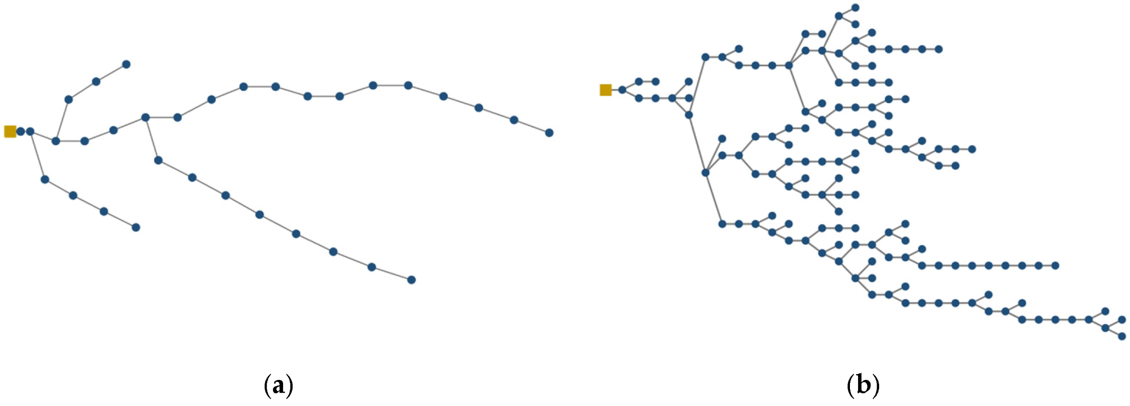
To evaluate the scalability of the proposed method, we employ two test systems of different scales. Their network topologies within the MAPDN environment are illustrated in Figure 4. The small-scale case is based on the IEEE 33-bus system, comprising 33 buses and 6 PV inverters (each modeled as an independent agent) partitioned into 4 electrical regions. For the medium-scale case, we use the IEEE 141-bus system, consisting of 141 buses and 22 PV inverters (acting as 22 agents) distributed across 9 regions. Both systems operate in a radial configuration with the substation as the slack bus and a 3-min control interval. The complete network case files (line and bus parameters, PV-inverter siting and capacity, and electrical-region partitioning) are provided as part of the open-source MAPDN benchmark [8] (https://github.com/Future-Power-Networks/MAPDN, accessed on 9 May 2026). Load profiles are derived from three years of electricity consumption records of 370 Portuguese households, while PV generation data are sourced from real-world operating logs of solar plants across ten regions; both datasets are released together with MAPDN [8] and are resampled to 3-min resolution. The same training/testing splits as in [8] are adopted for reproducibility.

5.1.2. Experimental Comparison Methods

To comprehensively evaluate PST-MA, we benchmark it against four representative MARL baselines, encompassing classical actor–critic methods, policy optimization algorithms, and recent graph-based variants. To ensure a fair comparison, all methods employ parameter sharing and are trained under identical environmental configurations and reward designs. Each method is executed with five random seeds, and the aggregated statistics across these runs are reported.

(1)

GKAN-MA is a recently proposed graph-attention-based MARL framework enhanced by a Kolmogorov–Arnold Network (KAN) value head. It introduces GATv2 into the MADDPG backbone and replaces the conventional value head with learnable B-spline basis functions. As a graph-based baseline, it is particularly relevant for assessing the incremental contribution of our proposed design [41].

(2)

MADDPG employs an actor–critic architecture under the CTDE paradigm. Each agent operates a decentralized actor driven by local observations and a centralized critic conditioned on joint information. It is the standard continuous control baseline within the MAPDN environment and serves as the foundational paradigm for our method [15].

(3)

MATD3 extends the actor–critic framework with twin critics and target policy smoothing, which helps mitigate Q-value overestimation in complex multi-agent environments [42].

(4)

MAPPO extends Proximal Policy Optimization (PPO) to the multi-agent setting by using a shared centralized value function during training. It serves as a strong policy optimization baseline in cooperative MARL [24].

(5)

OPF is a centralized model-based optimization baseline that does not involve learning. At each control interval, it directly solves a reactive-power optimization problem using full network parameters and global bus measurements, subject to AC power-flow equations and inverter capability constraints. It serves as a non-learning model-based reference for comparison with the MARL methods [3].

5.1.3. Evaluation Metrics

We adopt three evaluation metrics that are standard in the AVC literature.

Controllable ratio (CR) is the primary safety metric. A time step is regarded as fully controllable if and only if all bus voltages lie within the safe interval $\left[0.95,1.05\right]$ p.u. The episode-level CR is the proportion of fully controllable time steps. A higher CR indicates a stronger ability to maintain voltage safety.

Power Loss (PL), the primary economic metric, is defined as the average sum of active power losses across all distribution lines per time step. It quantifies the impact of reactive power regulation on overall power transfer efficiency. Under comparable voltage regulation performance, a lower PL indicates better operational economy.

Node Voltage (NV) is employed for qualitative visualization. Typical test-day results are presented as bus voltage heatmaps, where the horizontal axis represents the bus index, the vertical axis represents the time step, and the color indicates the voltage magnitude. A voltage distribution that concentrates around 1.0 p.u. and exhibits greater spatial uniformity indicates more effective mitigation of voltage fluctuations.

5.1.4. Other Settings

Algorithms are trained with a policy learning rate and value learning rate, both set to 1.0 × 10⁻⁴. Using an experience replay buffer of size 5000 and sample batches of 32 transitions for each update. The voltage control task enforces a safety boundary of [0.95, 1.05] p.u., ensuring all node voltages remain within this operational range during training and evaluation. The specific parameter settings for PST-MA are presented in

Table 1. Parameter settings of PST-MA.

Parameters	Values
	33-Bus	141-Bus
GATv2 attention heads	2	4
GATv2 head dimension	64	32
GATv2 dropout rate	0.2	0.4
Electrical neighborhood size (k)	2	6
Electrical-distance attention bias	0.08	0.1
MTLA embedding dimension	128	128
MTLA attention heads	2	2
MTLA downsampling rate	2	2
MTLA dropout rate	0.1	0.1

. All algorithms were implemented in Python 3.9 using the PyTorch deep learning framework version 1.12.0. The experiments were conducted on a workstation equipped with an NVIDIA RTX 4090 GPU(NVIDIA Corporation, Santa Clara, CA, USA).

5.2. Performance in Benchmark Scenarios

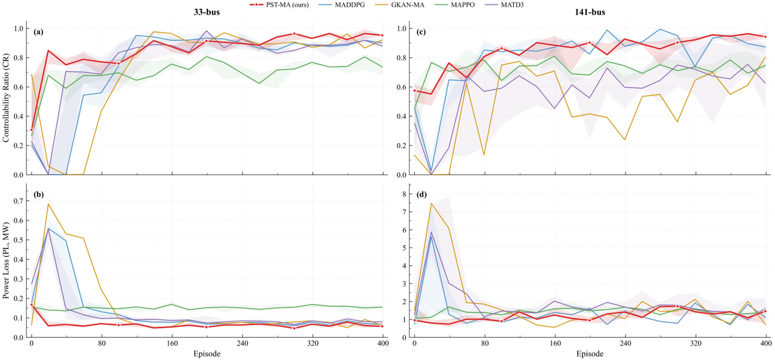
This section compares the training trajectories of all methods in the 33-bus and 141-bus systems. During training, the current policy is evaluated every fixed number of episodes, and the resulting controllable ratio (CR) and power loss (PL) are recorded. All methods are trained with five random seeds. The evaluation curves are reported as median trajectories, and the shaded areas denote the interquartile range (25th–75th percentile). In addition to the training curves shown in Figure 5,

Table 2. Median CR and PL of all methods in the 33-bus and 141-bus systems.

Methods	33-Bus		141-Bus
	CR	PL	CR	PL
PST-MA	0.9523	0.0563	0.9427	1.4564
GKAN-MA	0.9205	0.0623	0.8033	0.7192
MADDPG	0.9004	0.0672	0.8724	1.1071
MATD3	0.8795	0.0790	0.6255	1.6065
MAPPO	0.7364	0.1550	0.7469	1.4043

Note: Bold values indicate the best performance in each column, and underlined values indicate the second-best performance. For CR, higher values are better; for PL, lower values are better.

reports the median CR and PL achieved by each method in the two benchmark systems, which provides a compact view of the final performance.

Figure 5 and Table 2 jointly show that all five methods gradually learn effective voltage-regulation policies in the 33-bus system, but their convergence quality differs. According to Table 2, PST-MA achieves a median CR of 0.9523 and a median PL of 0.0563 MW, which are simultaneously the best safety and economy results among all compared methods. This observation agrees with Figure 5a, where the CR curve of PST-MA rises rapidly in the early stage, stabilizes in the middle and late stages, and exhibits a relatively narrow interquartile range, indicating good consistency across random seeds. GKAN-MA and MADDPG also reach high CR values, but both their final CR and PL remain inferior to PST-MA. The performance gap between PST-MA and GKAN-MA shows that graph attention alone is not sufficient; explicit physics-informed injection, spatiotemporal decoupling, and fine-grained credit assignment bring additional benefits. MATD3 exhibits more noticeable fluctuation and a higher PL of 0.0790 MW, whereas MAPPO converges smoothly but only reaches a CR of 0.7364. Overall, PST-MA achieves both the highest CR and the lowest PL in the small-scale scenario.

The 141-bus system is considerably more challenging because it contains more buses and more agents, leading to stronger and more complicated electrical coupling. Figure 5c shows that the CR of every method decreases to some extent as the scale grows, yet Table 2 confirms that PST-MA still attains the best median CR, 0.9427. Relative to GKAN-MA, MADDPG, MATD3, and MAPPO, the CR gain is 0.1394, 0.0703, 0.3172, and 0.1958, respectively. Although the PL of PST-MA is 1.4564 MW and is therefore not the lowest in Table 2, it remains below MATD3 and is accompanied by a markedly higher level of voltage security. This trade-off is also consistent with Figure 5d, where PST-MA maintains a competitive PL while keeping a clear advantage in CR. Notably, GKAN-MA attains the lowest PL (0.7192 MW) but only a CR of 0.8033, which suggests that introducing graph attention without deeper physical integration and refined credit assignment does not reliably translate into superior controllability in large-scale coupled systems. MADDPG remains competitive with a CR of 0.8724, but its safety performance is still lower than that of PST-MA. MATD3 shows the strongest instability, and MAPPO remains substantially behind PST-MA. Taken together, Figure 5 and Table 2 indicate that, in the larger system, the primary advantage of PST-MA lies in obtaining a higher and more stable level of voltage security at an acceptable economic cost.

5.3. Analysis on a Typical Test Day

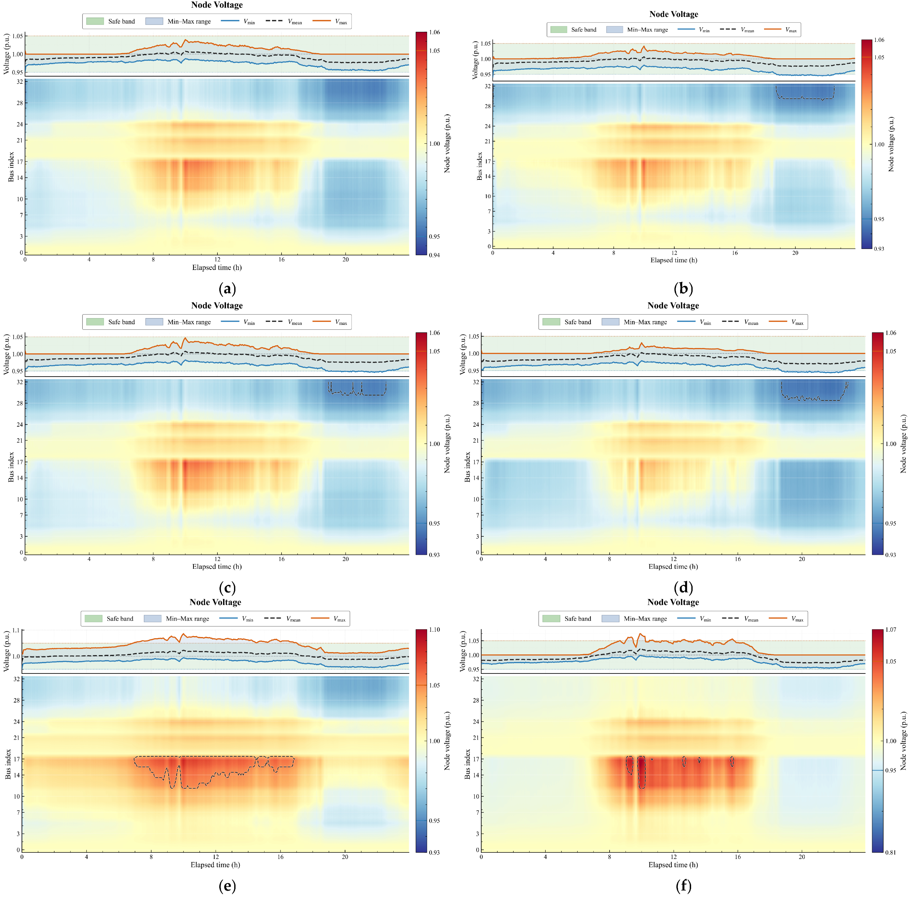
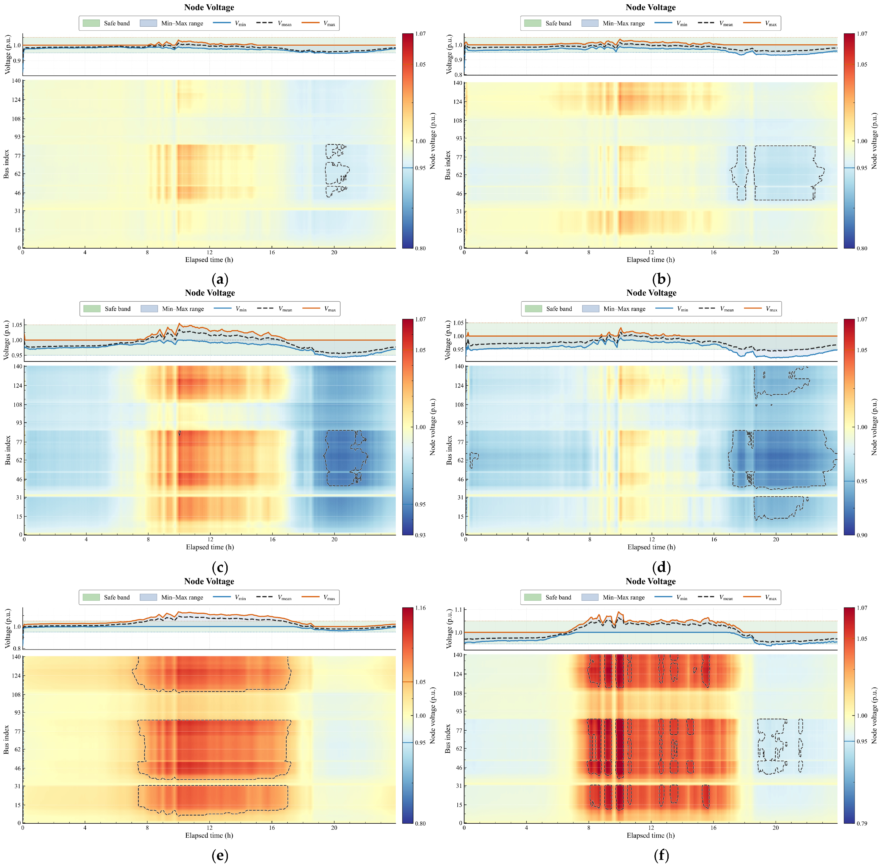
To further evaluate the practical control effect of the trained policies, a typical summer day (Day 199) with high PV output is selected for detailed analysis. Day 199 is a 24-h profile drawn from the held-out testing split of the MAPDN dataset [8]; with the 3-min control resolution it contains 480 consecutive control steps. The per-region PV curves exhibit a single midday peak (close to the rated inverter capacity around 11:00–13:00) while household load remains comparatively low during daytime, producing strong reverse power flow toward the substation and is the main driver of the feeder-end overvoltage analyzed below. During testing, all MARL methods use deterministic policies. In addition, a centralized OPF baseline is included as a non-learning, model-based point of comparison: at every control step it has full access to the network parameters and global bus measurements and solves a single-snapshot reactive-power optimization on the spot. The results are presented as voltage heatmaps, each consisting of an upper panel that shows voltage envelopes together with the safe band [0.95, 1.05] p.u., and a lower panel that shows a bus–time heatmap of voltage magnitudes. Dashed contours indicate voltage-limit violations.

5.3.1. Results in the 33-Bus System

Figure 6 shows the node-voltage heatmaps of the five methods in the 33-bus system. Overall, PST-MA, GKAN-MA, MADDPG, and MATD3 exhibit similar voltage patterns. Most bus voltages remain within the safe range during most time steps, and only mild voltage rise appears around the feeder end (approximately Buses 10–24) during the PV peak period from about 8 h to 14 h. From the upper-envelope panel, the voltage trajectories of these four methods remain close to, but generally below, the upper limit of 1.05 p.u. Among them, PST-MA exhibits a slightly smaller high-voltage region in both intensity and spatial extent, which indicates somewhat stronger suppression of voltage excursions. Nevertheless, differences among these four methods are still limited in the small-scale network.

By contrast, MAPPO behaves substantially worse than the other four methods. As shown in Figure 6e, its voltage envelope rises to about 1.09 p.u. during the PV peak period, clearly exceeding the safety limit. The heatmap also shows a broad orange-to-red region around Buses 10–24, together with visible violation contours, which indicates that MAPPO fails to effectively suppress the overvoltage caused by high PV injection. This observation is consistent with the lower CR observed during training. In short, because 33-bus is a relatively small-scale scenario, several CTDE-based methods can already learn reasonably effective control policies, and the performance differences become much more evident in the larger system.

The centralized OPF in Figure 6f is reported here as a model-based reference rather than as a competing controller, since it operates with full observability of the network state and explicit knowledge of the AC power-flow model at every control step. Even with this idealized information access, its upper envelope still briefly exceeds 1.05 p.u. around 9–10 h and small violation contours appear at the feeder end (Buses 14–17) during the PV peak, reflecting the well-known limitation that a single-snapshot dispatch cannot fully eliminate overvoltage when reverse power flow is strongest and inverter reactive capacity is tight. Against this reference, Operating in a fully decentralized manner at execution, PST-MA achieves an upper voltage envelope comparable to that of the centralized OPF solution. This indicates that, already in this small-scale scenario, the proposed framework is able to attain the performance level of a centralized model-based optimizer without requiring online optimization or global state knowledge.

5.3.2. Results in the 141-Bus System

Figure 7 presents the node-voltage heatmaps in the 141-bus system. Compared with the 33-bus case, this system contains 141 buses and 22 agents; so, electrical coupling is considerably more complex and the differences among methods become much more pronounced.

As shown in Figure 7a, PST-MA produces a relatively uniform green-to-light-yellow heatmap. The upper envelope remains below 1.05 p.u., and voltages stay above 0.95 p.u. for the vast majority of time steps. During the PV peak period from roughly 9 h to 14 h, some voltage rise appears in the regions around Buses 46–80 and Buses 120–130, yet the magnitude remains controllable and no large-scale violations are formed. This result indicates that the combination of local electrical graph construction, temporal history compression, and node-conditional value learning coordinates the reactive-power outputs of multiple inverters effectively in the larger network.

The baselines display different types of voltage violations. GKAN-MA is close to PST-MA during the PV peak, but a noticeable low-voltage violation appears in the region around Buses 40–80 after 14 h, suggesting insufficient coordination after PV output falls. MADDPG exhibits a bidirectional failure pattern—overvoltage during the day and undervoltage at night—especially around Buses 46–80 after 18 h. MATD3 alleviates daytime overvoltage to some extent, yet widespread low-voltage violations remain for multiple bus segments throughout the day. MAPPO performs the worst: during the peak period, the upper envelope rises to approximately 1.12–1.13 p.u., and the heatmap turns deep red over a large portion of the network. These observations are consistent with the training-stage comparison and confirm that the advantage of PST-MA becomes much clearer as network scale and coordination difficulty increase.

The contrast with the centralized OPF reference is particularly informative in the larger 141-bus system. Although OPF still benefits from full network observability at every step, Figure 7f shows that its upper envelope rises to roughly 1.08 p.u. during the PV peak (8–16 h), with clear overvoltage bands around Buses 15–30, 46–77, and 108–130 and additional low-voltage contours around Buses 46–77 after 18 h. This degradation reflects a structural limitation of single-snapshot centralized optimization—as already noted in Section 1, when the system is strongly coupled and inverter reactive capacity is tight, the per-step optimum can no longer satisfy all bus voltage constraints simultaneously. PST-MA, in contrast, maintains a markedly more uniform voltage profile within the safe band even in this much larger system. We attribute this advantage to the three coupled designs of PST-MA: physics-informed graph attention that aligns message passing with the actual electrical coupling rather than topology-only adjacency, temporal compression that stabilizes critic learning over the stacked observation history, and node-conditional value decoding that delivers a per-bus credit signal to each agent. Together, these mechanisms allow PST-MA to surpass the centralized model-based reference in larger and more strongly coupled scenarios while remaining fully decentralized at execution.

5.4. Ablation Study

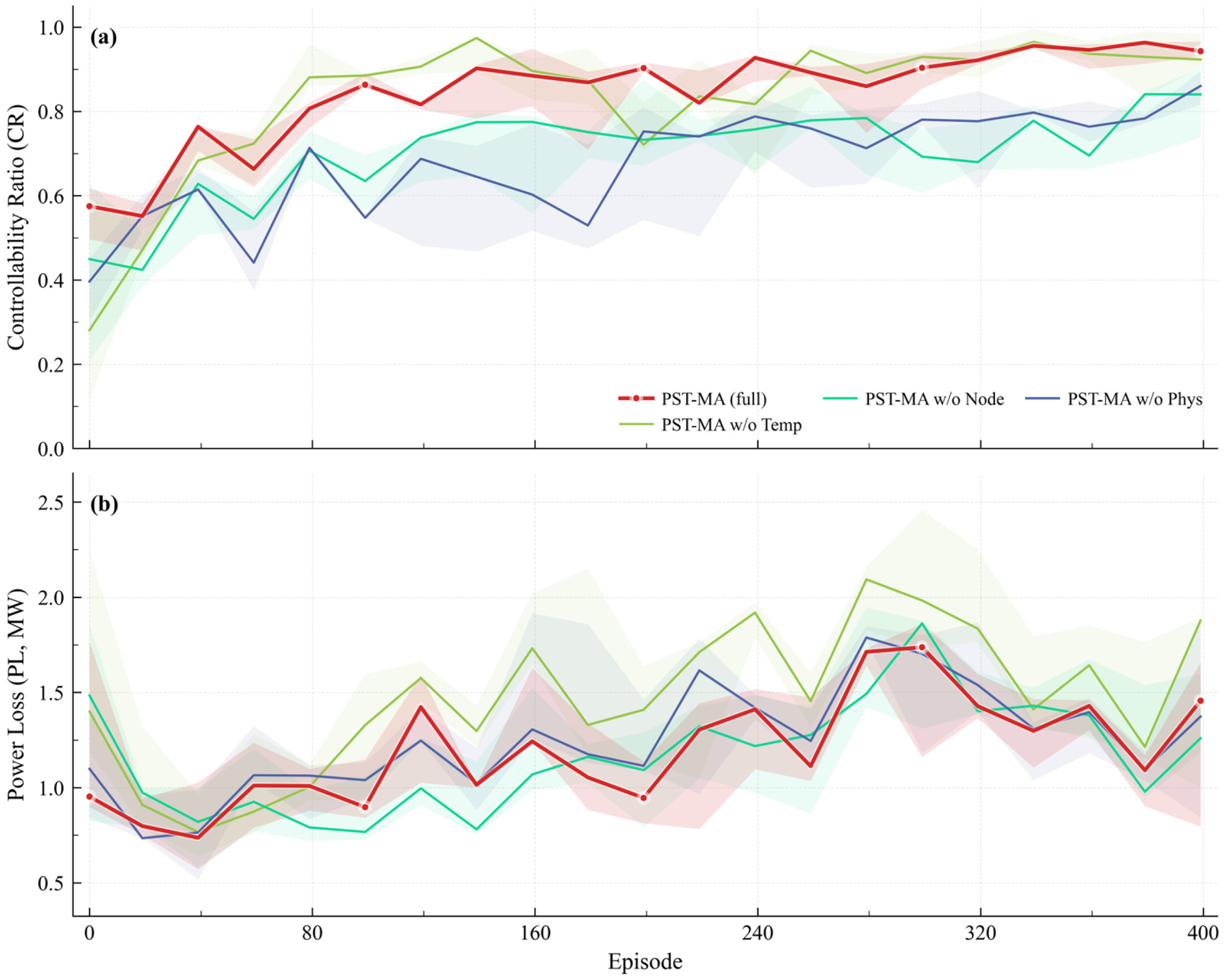
To quantify the contribution of each component, three ablation variants are tested in the 141-bus system: w/o Phys removes the physical-informed injection, w/o Temp removes temporal compression and late action fusion, and w/o Node removes node-conditional value output and spatial credit alignment. Their performance is compared with the full model. Results are reported as median curves with interquartile ranges.

As shown in Figure 8a, the performance of the full model improves steadily, converging to a CR of approximately 0.94 with the narrowest interquartile range (IQR). All three ablated variants experience performance degradation, albeit in distinct manners. The removal of the node-conditional value output (w/o Node) causes pronounced deterioration; its CR is consistently among the lowest throughout most of the training process, accompanied by significant variance. The reason that w/o Node is more damaging than w/o Temp can be traced to the credit-assignment structure: when the node-conditional head is removed, all agents share a single global Q-value; so, the deterministic-policy gradient seen by every actor is driven by the same scalar signal. Two consequences follow. Firstly, agents at electrically critical buses and those with marginal influence receive update signals of similar magnitude, contradicting the heterogeneous physical coupling of the network. Secondly, because all actor updates are pulled by a common scalar, their gradients become strongly correlated, which in non-stationary multi-agent training amplifies run-to-run variance. Removing the temporal module, by contrast, only changes the input representation while leaving the per-agent value decoding intact; so, its instability stems from early-stage representation noise that diminishes once the value function is fitted, whereas the deficiency of w/o Node is a structural credit-assignment bias that persists across the entire training horizon.

Eliminating the temporal compression module (w/o Temp) yields a rapid yet highly unstable learning trajectory. Although its CR increases rapidly initially—approaching 0.95 around Episode 120—it subsequently experiences sharp fluctuations and fails to maintain stability, despite remaining competitive in the later stages of training. Figure 8b illustrates a similar trend from an economic perspective; the w/o Temp variant exhibits the most severe active power loss (PL) oscillations, with peaks exceeding 2.0 MW. This behavior indicates that without learnable temporal compression and delayed action fusion, the critic network may converge rapidly initially but ultimately fails to establish stable value estimates.

Omitting the physics-informed injection (w/o Phys) leads to distinctly suboptimal performance, with the converged CR plateauing at approximately 0.87. Although it shows slight recovery in the later stages, a significant performance gap remains compared to the full model. This demonstrates the necessity of explicit physics-informed injection for the accurate modeling of electrical coupling. Overall, the three components of PST-MA are highly complementary: node-conditional value learning contributes substantially to final convergence, temporal compression is crucial for training stability, and physics-informed injection provides consistent performance gains.

6. Conclusions

In the paper we propose PST-MA, a physics-informed spatiotemporal value-learning framework for active voltage control in active distribution networks. This method enhances MARL in three key areas: physical-topology awareness, spatial credit assignment, and temporal modeling stability. Specifically, by incorporating line impedance and electrical distance into the graph attention mechanism, PST-MA aligns value learning with underlying electrical couplings. Furthermore, fine-grained per-agent credit assignment is achieved through node-conditional value outputs and gradient isolation. To ensure training stability, the framework decouples temporal encoding from action-gradient propagation utilizing temporal latent compression, gated bypass fusion, and late action fusion.

Evaluations on the IEEE 33-bus and 141-bus systems using the MAPDN platform demonstrate that PST-MA achieves the highest controllable ratio compared to baseline methods. Additionally, ablation studies verify the complementary nature of its three core components. In terms of computational cost, the focus-graph generation enlarges the effective critic batch from $B$ to $B$·$N$, scaling linearly with the number of agents $N$ and introducing a moderate per-update training overhead relative to a standard MARL critic that outputs a single global Q-value, while the actor-side inference cost remains identical to MADDPG since the electrical k-NN graph is built only once at start-up. Despite its efficacy, this study has certain limitations. The physics-informed graph relies on offline parameters and assumes a static topology, leaving topology reconfiguration and parameter uncertainties unaddressed. Real-grid deployment also raises practical issues beyond the scope of this paper, including communication latency and packet loss between inverters and the control layer, asynchronous regional measurement and actuation, and model–reality mismatch in line and inverter parameters. Future work will explore dynamic graph construction, latency-aware and asynchronous credit-assignment mechanisms, and extensions to hybrid action spaces accommodating heterogeneous controllable resources.

References

1. Kundur, P. Power system stability. In Power System Stability and Control; Taylor & Francis Group: Oxfordshire, UK, 2007; Volume 10, 218p. [Google Scholar]
2. Cao, D.; Hu, W.; Zhao, J.; Huang, Q.; Chen, Z.; Blaabjerg, F. A multi-agent deep reinforcement learning based voltage regulation using coordinated PV inverters. IEEE Trans. Power Syst. 2020, 35, 4120–4123. [Google Scholar] [CrossRef]
3. Agalgaonkar, Y.P.; Pal, B.C.; Jabr, R.A. Distribution voltage control considering the impact of PV generation on tap changers and autonomous regulators. IEEE Trans. Power Syst. 2013, 29, 182–192. [Google Scholar] [CrossRef]
4. Wu, J.; Wang, Z.; Han, J.; Li, Q.; Sun, R.; Li, C.; Cheng, Y.; Zhou, B.; Guo, J.; Long, B. A Novel Data-Driven Multi-Agent Reinforcement Learning Approach for Voltage Control Under Weak Grid Support. Sensors 2025, 25, 7399. [Google Scholar] [CrossRef] [PubMed]
5. Su, S.; Zhan, H.; Zhang, L.; Xie, Q.; Si, R.; Dai, Y.; Gao, T.; Wu, L.; Zhang, J.; Shang, L. Volt-VAR control in active distribution networks using multi-agent reinforcement learning. Electronics 2024, 13, 1971. [Google Scholar] [CrossRef]
6. Zhang, L.; Yang, F.; Yan, D.; Qian, G.; Li, J.; Shi, X.; Xu, J.; Wei, M.; Ji, H.; Yu, H. Multi-agent deep reinforcement learning-based distributed voltage control of flexible distribution networks with soft open points. Energies 2024, 17, 5244. [Google Scholar] [CrossRef]
7. Wei, H.; Chang, S.; Zhang, J. Graph-Based topological embedding and deep reinforcement learning for autonomous voltage control in power system. Sensors 2025, 25, 733. [Google Scholar] [CrossRef] [PubMed]
8. Wang, J.; Xu, W.; Gu, Y.; Song, W.; Green, T.C. Multi-agent reinforcement learning for active voltage control on power distribution networks. Adv. Neural Inf. Process. Syst. 2021, 34, 3271–3284. [Google Scholar]
9. Wu, Z.; Li, Y.; Gu, W.; Dong, Z.; Zhao, J.; Liu, W.; Zhang, X.P.; Liu, P.; Sun, Q. Multi-timescale voltage control for distribution system based on multi-agent deep reinforcement learning. Int. J. Electr. Power Energy Syst. 2023, 147, 108830. [Google Scholar] [CrossRef]
10. Luo, F.; Wang, S.; Lv, Y.; Mu, R.; Fo, J.; Zhang, T.; Xu, J.; Wang, C. Domain knowledge-enhanced graph reinforcement learning method for Volt/Var control in distribution networks. Appl. Energy 2025, 398, 126409. [Google Scholar] [CrossRef]
11. Qu, Y.; Ma, J.; Wu, F. Safety constrained multi-agent reinforcement learning for active voltage control. arXiv 2024, arXiv:2405.08443. [Google Scholar] [CrossRef]
12. Hu, D.; Li, Z.; Ye, Z.; Peng, Y.; Xi, W.; Cai, T. Multi-agent graph reinforcement learning for decentralized Volt-VAR control in power distribution systems. Int. J. Electr. Power Energy Syst. 2024, 155, 109531. [Google Scholar] [CrossRef]
13. Mu, C.; Liu, Z.; Yan, J.; Jia, H.; Zhang, X. Graph multi-agent reinforcement learning for inverter-based active voltage control. IEEE Trans. Smart Grid 2023, 15, 1399–1409. [Google Scholar] [CrossRef]
14. Zhang, B.; Cao, D.; Hu, W.; Ghias, A.M.; Chen, Z. Physics-Informed Multi-Agent deep reinforcement learning enabled distributed voltage control for active distribution network using PV inverters. Int. J. Electr. Power Energy Syst. 2024, 155, 109641. [Google Scholar] [CrossRef]
15. Lowe, R.; Wu, Y.; Tamar, A.; Harb, J.; Abbeel, P.; Mordatch, I. Multi-Agent Actor-Critic for Mixed Cooperative-Competitive Environments. In Proceedings of the 31st Conference on Neural Information Processing Systems (NIPS 2017), Long Beach, CA, USA, 4–9 December 2017; Volume 30. [Google Scholar] [CrossRef]
16. Oroojlooy, A.; Hajinezhad, D. A review of cooperative multi-agent deep reinforcement learning. Appl. Intell. 2023, 53, 13677–13722. [Google Scholar] [CrossRef]
17. Chen, R.; Tan, Y. Credit assignment with predictive contribution measurement in multi-agent reinforcement learning. Neural Netw. 2023, 164, 681–690. [Google Scholar] [CrossRef] [PubMed]
18. Liang, Y.; Wu, H.; Wang, H.; Cai, H. Asynchronous credit assignment for multi-agent reinforcement learning. arXiv 2024, arXiv:2408.03692. [Google Scholar]
19. Liu, K.; Zhang, T.; Xu, X.; Zhao, Y. Counterfactual value decomposition for cooperative multi-agent reinforcement learning. Neural Netw. 2025, 190, 107692. [Google Scholar] [CrossRef]
20. Hausknecht, M.J.; Stone, P. Deep Recurrent Q-Learning for Partially Observable MDPs. In AAAI Fall Symposia; The University of Texas at Austin: Austin, TX, USA, 2015; Volume 45, p. 141. [Google Scholar]
21. Deng, K.; Woodland, P.C. Multi-head Temporal Latent Attention. arXiv 2025, arXiv:2505.13544. [Google Scholar] [CrossRef]
22. Li, X.; Xue, S.; He, Z.; Shi, H. TMAC: A Transformer-based partially observable multi-agent communication method. PeerJ Comput. Sci. 2025, 11, e2758. [Google Scholar] [CrossRef]
23. Li, Z.; Wu, L.; Su, K.; Wu, W.; Jing, Y.; Wu, T.; Duan, W.; Yue, X.; Tong, X.; Han, Y. Coordination as inference in multi-agent reinforcement learning. Neural Netw. 2024, 172, 106101. [Google Scholar] [CrossRef]
24. Yu, C.; Velu, A.; Vinitsky, E.; Gao, J.; Wang, Y.; Bayen, A.; Wu, Y. The surprising effectiveness of ppo in cooperative multi-agent games. Adv. Neural Inf. Process. Syst. 2022, 35, 24611–24624. [Google Scholar]
25. Hua, D.; Peng, F.; Liu, S.; Lin, Q.; Fan, J.; Li, Q. Coordinated volt/var control in distribution networks considering demand response via safe deep reinforcement learning. Energies 2025, 18, 333. [Google Scholar] [CrossRef]
26. Murugesan, A.; Durgadevi, K.; Contractor, D.; Rathod, Y. Machine learning-driven intelligent voltage control in renewable energy grids. Electr. Power Syst. Res. 2025, 248, 111869. [Google Scholar] [CrossRef]
27. Zhang, Y.; Yue, M.; Wang, J.; Yoo, S. Multi-agent graph-attention deep reinforcement learning for post-contingency grid emergency voltage control. IEEE Trans. Neural Netw. Learn. Syst. 2024, 35, 3340–3350. [Google Scholar] [CrossRef]
28. Zhang, X.; Gui, X.; Sun, P.; Li, X.; Zhang, Y.; Wang, X.; Dang, C.; Liu, X. Reactive Power Optimization of a Distribution Network Based on Graph Security Reinforcement Learning. Appl. Sci. 2025, 15, 8209. [Google Scholar] [CrossRef]
29. Brody, S.; Alon, U.; Yahav, E. How attentive are graph attention networks? arXiv 2021, arXiv:2105.14491. [Google Scholar]
30. Su, T.; Zhao, J.; Pei, Y.; Ding, F. Probabilistic physics-informed graph convolutional network for active distribution system voltage prediction. IEEE Trans. Power Syst. 2023, 38, 5969–5972. [Google Scholar] [CrossRef]
31. Hong, Z.W.; Su, S.Y.; Shann, T.Y.; Chang, Y.H.; Lee, C.Y. A deep policy inference q-network for multi-agent systems. arXiv 2017, arXiv:1712.07893. [Google Scholar]
32. Rashid, T.; Samvelyan, M.; De Witt, C.S.; Farquhar, G.; Foerster, J.; Whiteson, S. Monotonic value function factorisation for deep multi-agent reinforcement learning. J. Mach. Learn. Res. 2020, 21, 1–51. [Google Scholar]
33. Ngo, Q.H.; Nguyen, B.L.; Vu, T.V.; Zhang, J.; Ngo, T. Physics-informed graphical neural network for power system state estimation. Appl. Energy 2024, 358, 122602. [Google Scholar] [CrossRef]
34. Sunehag, P.; Lever, G.; Gruslys, A.; Czarnecki, W.M.; Zambaldi, V.; Jaderberg, M.; Lanctot, M.; Sonnerat, N.; Leibo, J.Z.; Tuyls, K.; et al. Value-decomposition networks for cooperative multi-agent learning. arXiv 2017, arXiv:1706.05296. [Google Scholar]
35. Wang, J.; Ren, Z.; Han, B.; Ye, J.; Zhang, C. Towards understanding cooperative multi-agent q-learning with value factorization. Adv. Neural Inf. Process. Syst. 2021, 34, 29142–29155. [Google Scholar]
36. Son, K.; Kim, D.; Kang, W.J.; Hostallero, D.E.; Yi, Y. Qtran: Learning to factorize with transformation for cooperative multi-agent reinforcement learning. In Proceedings of the 36th International Conference on Machine Learning, Long Beach, CA, USA, 9–15 June 2019; pp. 5887–5896. [Google Scholar]
37. Foerster, J.; Farquhar, G.; Afouras, T.; Nardelli, N.; Whiteson, S. Counterfactual multi-agent policy gradients. Proc. AAAI Conf. Artif. Intell. 2018, 32, 11794. [Google Scholar] [CrossRef]
38. Li, J.; Kuang, K.; Wang, B.; Liu, F.; Chen, L.; Fan, C.; Wu, F.; Xiao, J. Deconfounded value decomposition for multi-agent reinforcement learning. In Proceedings of the 39th International Conference on Machine Learning, Baltimore, MD, USA, 17–23 July 2022; PMLR: Baltimore, MD, USA, 2022; pp. 12843–12856. [Google Scholar]
39. Wu, X.; Zhu, Y.; Chen, C.; Chen, C. GCM: Interpretable Multiagent Reinforcement Learning via Graph Cooperation Modeling. IEEE Trans. Neural Netw. Learn. Syst. 2026, 37, 1823–1837. [Google Scholar] [CrossRef]
40. Choi, Y.; Di Marco, P.; Park, P. Communication-Aware Graph Neural Network for Multi-Agent Reinforcement Learning. IEEE Access 2025, 13, 55832–55840. [Google Scholar] [CrossRef]
41. Sun, L.; Xiao, H.; Qi, S.; Li, H.; Zhang, J.; Wang, X. KAN-Enhanced Graph Learning for Active Voltage Control in Dynamic Power Systems. In Proceedings of the 25th International Conference on Autonomous Agents and Multiagent Systems, Paphos, Cyprus, 25–29 May 2026. [Google Scholar]
42. Ackermann, J.; Gabler, V.; Osa, T.; Sugiyama, M. Reducing overestimation bias in multi-agent domains using double centralized critics. arXiv 2019, arXiv:1910.01465. [Google Scholar] [CrossRef]
Figure 1. Topological partitioning of the IEEE 33-bus distribution system. Numbered circles represent the system buses. Based on the shortest paths from the terminal buses to the main feeder (buses 1–6), the system is partitioned into four control regions. Buses 2–33 are targeted for voltage control, whereas buses 0–1 represent the substation and the upstream grid, acting as slack buses with a constant voltage magnitude and unlimited active and reactive power support. Additionally, G represents the external generator, L denotes the electrical loads, and PV indicates the locations of photovoltaic units.
Applsci 16 05109 g001
Figure 2. Framework of the proposed physics-informed spatiotemporal multi-agent value-learning method (PST-MA) on the 33-bus system. The method follows centralized training and decentralized execution (CTDE). A shared gated recurrent unit (GRU) actor performs decentralized control, while the centralized critic integrates temporal encoding, physics-informed spatial graph encoding, and node-conditional Q-value decoding to achieve spatiotemporal value learning and fine-grained credit assignment. Here, B attn denotes the electrical-distance attention-bias matrix; darker shades schematically indicate stronger relative bias toward electrically closer nodes.
Applsci 16 05109 g002
Figure 3. Critic-side observation encoding architecture with temporal compression and delayed action fusion. The diagram shows the encoding pipeline for a representative agent node, including temporal compression, current-frame bypass, gated fusion, and delayed action injection. Colors and shaded blocks distinguish functional modules, solid arrows indicate data flow, and the dashed path denotes the action-gradient route that bypasses the temporal encoder.
Applsci 16 05109 g003
Figure 4. Topologies of the 33-bus and 141-bus distribution networks within the Multi-Agent Power Distribution Network (MAPDN) environment. (a) 33-bus network; (b) 141-bus network. Blue circles indicate buses, yellow squares indicate the substation, and lines indicate distribution branches.
Applsci 16 05109 g004
Figure 5. Evaluation results during training in the 33-bus and 141-bus systems. Panels (a,c) show the CR curves for the two systems, whereas Panels (b,d) show the PL curves (MW). Solid lines denote the median over five seeds, and shaded regions denote the interquartile range (25th–75th percentile).
Applsci 16 05109 g005
Figure 6. Test results of all methods in the 33-bus system under the representative summer scenario. (a) PST-MA; (b) GKAN-MA; (c) MADDPG; (d) MATD3; (e) MAPPO; and (f) OPF.
Applsci 16 05109 g006
Figure 7. Test results of all methods in the 141-bus system under the representative summer scenario. (a) PST-MA; (b) GKAN-MA; (c) MADDPG; (d) MATD3; (e) MAPPO; and (f) OPF.
Applsci 16 05109 g007
Figure 8. Training-evaluation results of the ablation study in the 141-bus system. (a) CR; (b) PL (MW).Solid lines denote the median over five seeds, and shaded regions denote the interquartile range (25th–75th percentile). Here, w/o denotes “without”.
Applsci 16 05109 g008