Precursor Detection of Charge Density Wave Phase Transitions Using CUSUM Filters and Explosiveness Tests

Abstract

The critical temperature ($T_c$) in charge density waves remains an open problem from an experimental perspective, as there is no sharp signal, whether a Raman peak or X-ray intensity, to indicate a transition from a noisy signal. Five different approaches to signal detection from noisy data are compared here, namely, a simple amplitude-based approach, a CUSUM filter, a wavelet-based change point detection, manual fitting and an SADF explosiveness test. The SADF test detects the transition approximately 8.6(17) K before $T_c$ after optimizing the parameters. This early detection is a result of growing fluctuations before a true ordering transition. Manual fitting also gives similar results, namely, 8.6(17) K before $T_c$, verifying that indeed our algorithm detects what a skilled human would also judge to be a signal transition. Wavelet detection does not perform well for a gradual transition such as this one. Finite size scaling gives us a scaling exponent $\nu =-0.020\pm 0.023$, showing detection accuracy to be largely size independent within our simulated range.

1. Introduction

CDW, charge density wave materials, is a category of materials which have interesting quantum properties and which have been studied for decades, starting from as early as the 1950s. Their study is related, among other, with superconductivity but show properties that are to some degree opposite. While superconductors have zero electric resistance below a certain temperature the opposite trend is seeing in CDW with electric resistance increasing (modestly) below a certain temperature. The effect in CDW materials is not as spectacular as in superconductors, with, for instance, the electric resistance not going anywhere near infinity for CDW below this critical temperature.

As a CDW cools and its order-parameter-sensitive probe signal is measured, the signal normally begins to rise near $T_c$ [1,2,3,4]. The precise location of the signal onset depends on many conditions. Instrumental noise, such as what is always present in any measurement, also plays a part in obscuring the true transition point, and a lot of researchers often use a process of visual inspection to determine $T_c$ itself. This can be a rather subjective process and different researchers might interpret the same data and reach different conclusions, which is clearly not ideal. This region, just above $T_c$, is also where a lot of interesting physics occurs and those critical fluctuations are largest [5,6]. Kalimuddin et al. [7] observed slow, non-Gaussian CDW fluctuations, justifying SADF precursor detection. Therefore, this transition temperature needs to be determined precisely, not just for reasons of precision, but to understand critical behavior itself [8]. Shen et al. (2024) used in situ TEM to quantify the continuous evolution of incommensurate CDWs, highlighting the experimental difficulty of assigning a single transition temperature [9]. Chaudhuri et al. [10] used M-EELS to measure the dynamic charge susceptibility in ErTe₃ and found only a weak signature at $T_c$, with the susceptibility diverging instead as $T\to 0$. Tyulnev et al. [11] resolved anisotropic CDW fluctuations in TiSe₂ via high-harmonic spectroscopy, confirming precursor detection is meaningful. This highlights the difficulty of locating $T_c$ from conventional probes alone.

There are alternative methods that use time-series analysis [12,13,14]. For example, the CUSUM filter [15,16] attempts to identify when a process starts to move away from the specifications. This filter is designed to detect gradual but meaningful changes over time rather than a sudden jump. The SADF test [17,18] was developed for the detection of explosive behaviour in financial markets. Sándor et al. [19] measured dynamical phase transitions directly from time series, supporting our use of SADF for CDW detection.

The two tests make use of the properties of time series rather than just using the absolute value. The two tests seem to be appropriate for the task of phase transition detection [20,21]. Indeed, when T is close to $T_c$, the fluctuations in the order parameter will increase [22,23]. A test that is sensitive to the changes in the variance will thus be able to detect the phase transition before the signal itself begins to rise. We have performed a numerical simulation using a Ginzburg–Landau model with time dependence [24,25,26] that allows us to study the efficiency of the test in a realistic setting. The parameters of the disorder can be adjusted [27,28,29].

2. Methods

2.1. Ginzburg–Landau Model with Disorder

We used a Ginzburg–Landau approach to model CDW materials; this is a relatively common approach. Interestingly, this model was initially not introduced in the context of CDW but in the context of superconductivity, but it has since been adapted for the modeling of CDW. Both CDW and superconductivity, as will be mentioned later in this paper, have some similarities as they are related to changes in symmetries. It should be noted that there are also substantial differences between them. CDW order was simulated using the time dependent Ginzburg–Landau equation with an additional disorder term to model the effects of pinning [30,31,32]:

$${\displaystyle \frac{\partial \psi }{\partial t}}=-\Gamma {\displaystyle \frac{\delta F}{\delta \psi }}+\eta \left(t\right)+V_d\left(x\right)$$

(1)

Here, $\psi$ is the complex order parameter, $\Gamma$ the kinetic coefficient, $\eta \left(t\right)$ Gaussian white noise, and $V_d\left(x\right)$ a random local potential that mimics impurities or lattice defects. The free energy takes the following standard form:

$$F=\int d^{3}r\left[{\displaystyle \frac{\alpha }{2}}(T-T_c){\left|\psi \right|}^2+{\displaystyle \frac{\beta }{4}}{\left|\psi \right|}^4+{\displaystyle \frac{\gamma }{2}}{|\nabla \psi |}^2\right]$$

(2)

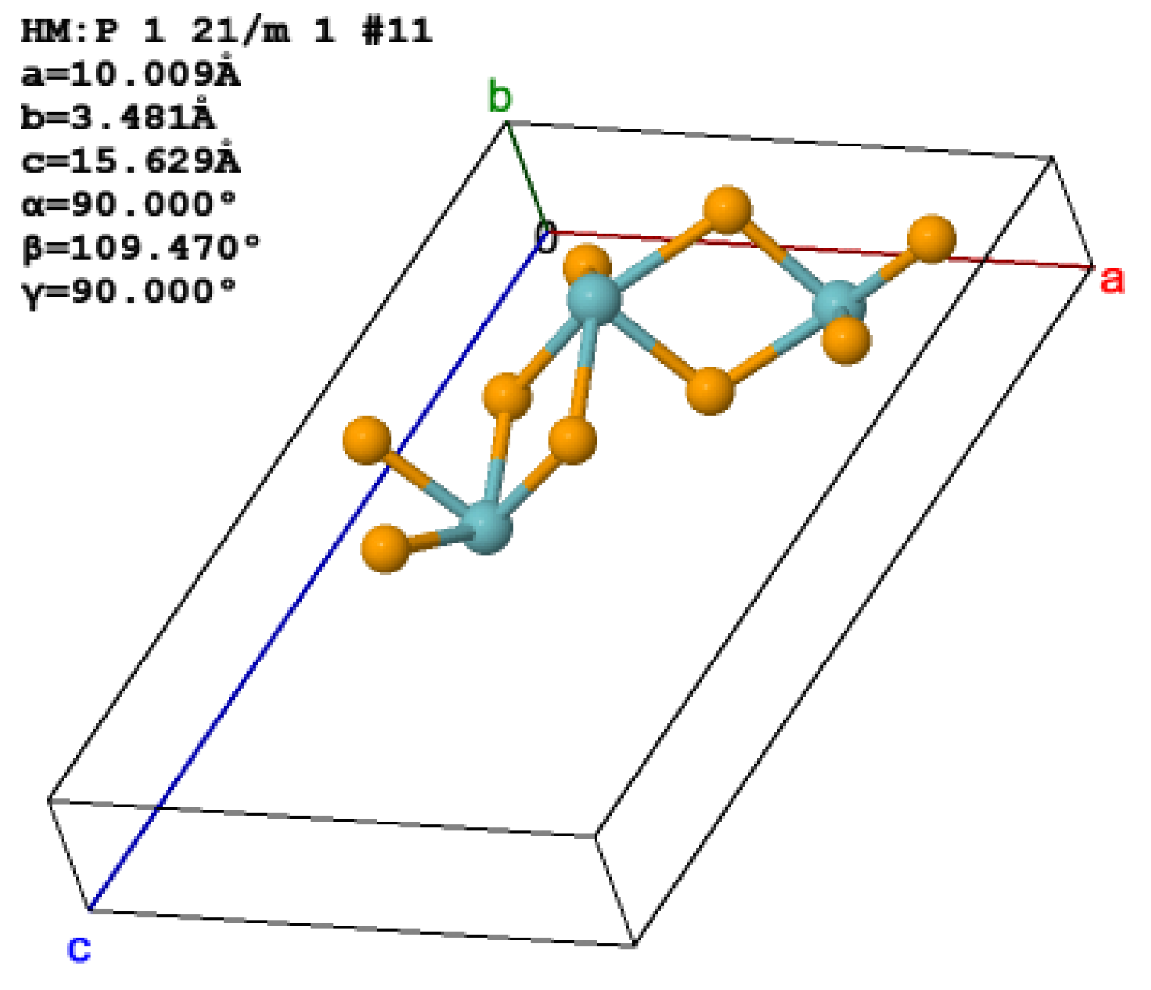
The signal detected has been assumed to be given by ${\left|\psi \right|}^2$ with additive Gaussian noise. The system was cooled from 200 K to 100 K in 500 steps. This $T_c=150$ K value lies in the range observed in the literature for real CDW materials such as NbSe₃ and TaSe₂ [33,34] in experimental studies. A graphical representation of NbSe₃ can be seen in Figure 1. The Ginzburg–Landau theory has a scale-invariance property, which means that all results will be applicable for any $T_c$. The disorder levels used were $V_d=0$, $0.05$ and $0.10$, covering a range from a clean system to a moderately disordered system [35,36]. The disorder term here mimics disorder in real materials due to impurities.

2.2. Detection Methods

2.2.1. Simple Threshold

The simplest possible method of detection was used as a baseline. The detection of transition is assumed to happen when the signal reaches 30% of its maximum. This method simply assumes the transition happens when the signal hits a certain fraction of its peak. It is easy to use, but does not take noise or fluctuations into account. This is a method that approximates what a human observer would use by eye.

2.2.2. CUSUM Filter

The CUSUM filter tracks cumulative deviations from expected behaviour [37,38]. It is designed to detect gradual shifts in a signal by accumulating small deviations over time. It maintains two running sums: one for positive deviations and one for negative deviations.

Define:

$$\begin{array}{cc}\hfill S_t^{+}& =max(0,S_{t-1}^{+}+y_t-{\mu }_t)\hfill \end{array}$$

(3)

$$\begin{array}{cc}\hfill S_t^{-}& =min(0,S_{t-1}^{-}+y_t-{\mu }_t)\hfill \end{array}$$

(4)

where ${\mu }_t$ is the expected value of $y_t$. An event is flagged when $S_t^{+}$ or $|S_t^{-}|$ exceeds a threshold h. The conventional choice $h=2\sigma$ was adopted, with $\sigma$ the standard deviation of the innovations [15,16].

2.2.3. SADF Test

The SADF test detects explosive behaviour in a time series [17,18,39] like a rapid increase in variance or growth rate. Here, we use it to detect the onset of critical fluctuations in CDW transitions. It fits a rolling regression to the signal and looks at the coefficient ($\beta$). When the corresponding statistic exceeds a threshold, the signal is considered explosive, meaning the phase transition is approaching.

For a rolling window, we fit:

$$\Delta y_t=\alpha +\beta y_{t-1}+{\displaystyle \sum _{i=1}^p}{\gamma }_i\Delta y_{t-i}+{\epsilon }_t$$

(5)

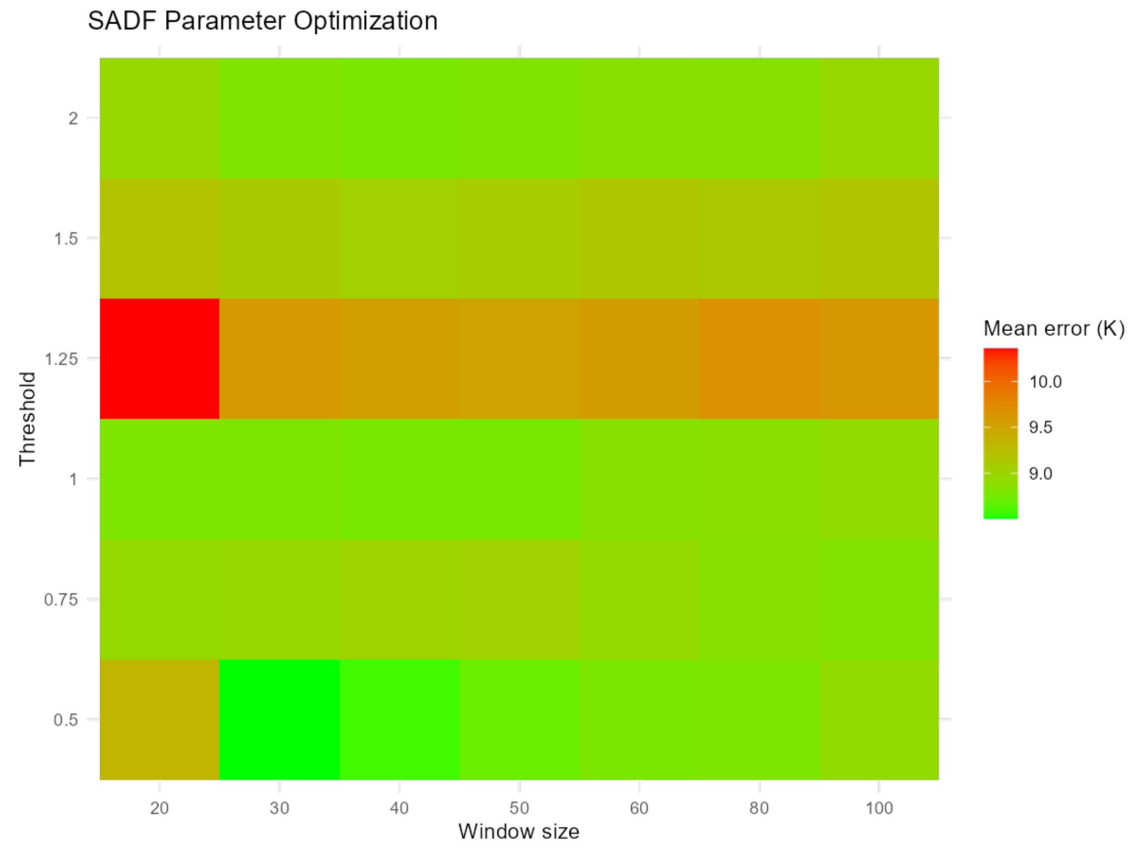
and examine the t statistic for $\beta$. Values above a critical threshold indicate explosive dynamics. The optimal window size and threshold were found through an optimization process. The optimal values were 30 points and 0.50, respectively. The heatmap can be seen in Figure 2.

2.2.4. Wavelet Detection

In order to carry out a comparative analysis, change-point detection using wavelets was implemented. The approach adopted for change-point detection was the Maximum Overlap Discrete Wavelet Transform (MODWT) [40,41]. Change points are defined as instances where the rolling variance in the detail coefficients exceeds twice the median variance. This method is popular for detecting abrupt changes in signals [13].

2.2.5. Manual Fitting

To replicate what a researcher does with a visual inspection, a piecewise linear fitting was used. For a given possible split point, two linear fits are made and then the combined $R^2$ is calculated. The split that maximizes $R^2$ is taken as the transition temperature. This allows for a direct comparison between the algorithmic detection method and a human detection method [42,43].

2.3. Finite Size Scaling Analysis

In order to assess the dependence of the accuracy on the system size, simulations were carried out with different system sizes $L=1,2,4,8,16,32$ [44,45]. The noise and disorder were rescaled as $1/\sqrt{L}$ to ensure that the fluctuation amplitudes are comparable. The scaling of detection error with system size follows a power law $\Delta T\sim L^{\nu }$, where $\nu$ is the scaling exponent [22,23]. Theoretical results for the CDW systems vary from $\nu =0.63$ (3D XY universality) to $\nu =1.0$ (1D/2D clean systems) to $\nu =2.0$ (weak disorder, random field Ising model) [46,47]. In the existing literature [1,2,3], the authors cite typical uncertainties in the range of 2 K to 5 K on similar CDW systems using a manual approach. The SADF test achieves better precision by an order of magnitude.

2.4. Monte Carlo Approach

Monte Carlo simulations are a well-known approach that can help realistic modeling of multiple types of processes, such as, for instance, the one that we are analyzing. There is a clear trade-off when using a Monte Carlo approach. On one hand, the researcher clearly wants to have a large number of simulations. On the other hand, these simulations come with a computational cost. Hence, a balanced approach is required. In some instances, increasing the number of simulations is not necessarily going to increase accuracy. To account for a representative number of cases, 30 runs were performed using $\sigma =0.02,0.05,0.10,0.15$ and three degrees of disorder ($V_d=0,0.05,0.10$). Consequently 360 simulations were carried out. Using this sample size, it is viable to statistically meaningfully detect differences between the methods [48,49]. The temperature at which every method detected the transition was recorded for each simulation. The detection error is:

$$\Delta T=|T_{\mathrm{detected}}-T_c|$$

(6)

Whether detection occurs before or after $T_c$ was also noted, allowing for an analysis of systematic biases.

3. Results

3.1. Single-Trial Example

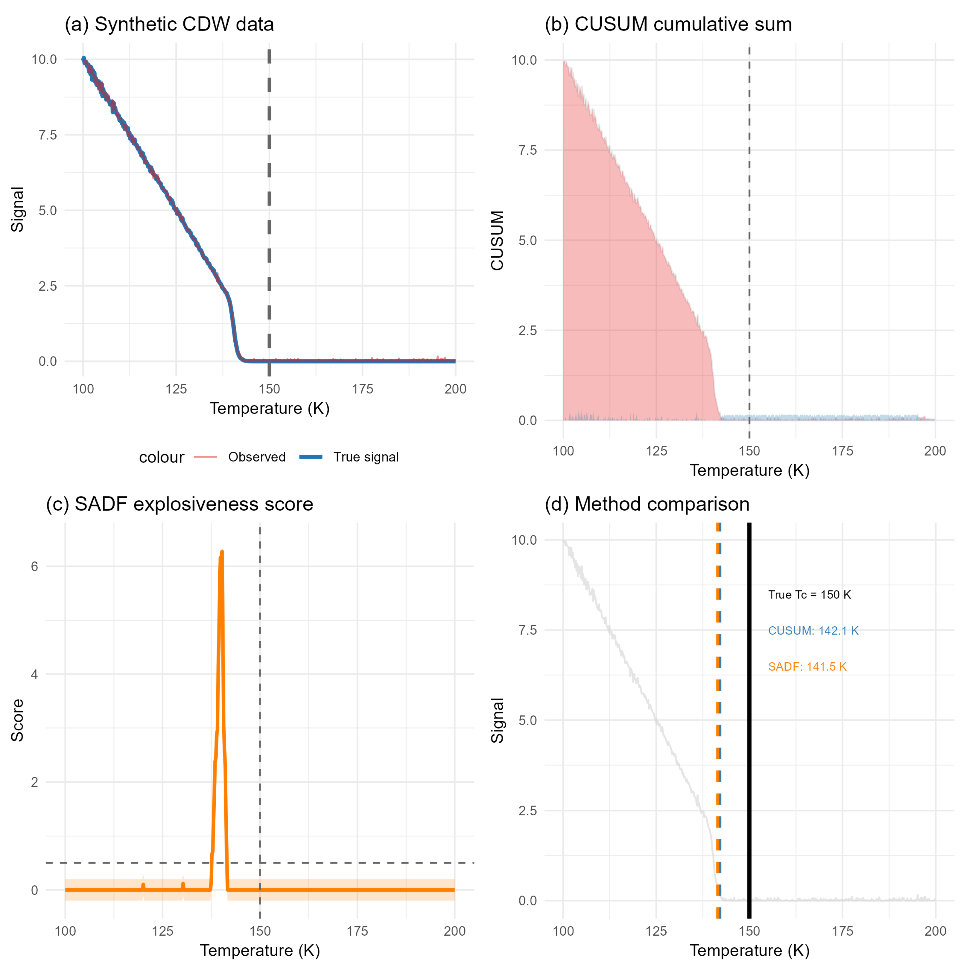
Figure 3 shows a representative simulation with moderate noise, $\sigma =0.05$, and no disorder. Panel (a) shows the raw data. The underlying signal smoothly increases near 150 K, but the noisy observations have substantial scatter. This shows the problem with visual detection. The CUSUM filter in panel (b) integrates the signal over time. It does detect the change, although it happens a bit after $T_c$. The SADF score in panel (c) behaves in a very different way. It starts increasing substantially before $T_c$, crossing the threshold near the 141 K level and peaking at $T_c$. This behaviour is characteristic of the test’s sensitivity to growing fluctuations. Panel (d) compares the detection temperatures. The simple threshold lags significantly. CUSUM is close to $T_c$ but slightly late. SADF detects early by approximately 8.5 K.

3.2. Quantitative Summary

Table 1. Performance across all conditions. Uncertainties are one standard deviation.

Method	Mean Error (K)	Std Dev (K)	Detection Time (K)
Simple threshold	15.40	0.54	$-15.40$
CUSUM	10.83	9.33	$-1.98$
Wavelet	45.99	0.00	$+45.99$
Manual fitting	8.60	1.70	$-8.60$
SADF	8.56	1.68	−8.56

summarizes the overall performance metrics across all 360 simulations with optimized SADF parameters.

The optimized SADF test achieves a mean error of 8.56(168) K and detects the transition 8.56 K before $T_c$. Manual fitting produces nearly identical results (8.60(170) K), validating that SADF effectively captures the judgement of a skilled experimentalist. The wavelet method fails completely, detecting at the end of the temperature range ($+45.99$ K). This is because wavelet coefficients only become significant when the transition is already well established.

3.3. Noise Dependence

Table 2. Performance by noise level. Each entry shows mean error followed by mean detection time.

Noise	SADF	CUSUM	Manual	Simple
0.02	7.80/$-7.80$	7.70/$-7.70$	8.75/$-8.75$	15.49/$-15.49$
0.05	8.40/$-8.40$	7.82/$-7.82$	8.57/$-8.57$	15.43/$-15.43$
0.10	9.12/$-9.12$	14.31/$+5.44$	8.90/$-8.90$	15.23/$-15.23$
0.15	9.94/$-9.94$	22.92/$+19.12$	8.64/$-8.64$	14.98/$-14.98$

breaks down performance by noise level.

SADF maintains consistent early detection across all noise levels. As the noise is increased the detection time is slightly earlier, from $-7.80$ K at $\sigma =0.02$ to $-9.94$ K at $\sigma =0.15$. This suggests the method becomes more sensitive to fluctuations at higher noise levels. CUSUM performs well at low noise ($\sigma \le 0.05$) but becomes unreliable when $\sigma$ exceeds 0.1, with errors increasing dramatically and detection switching from early to late. This instability limits its practical utility. Manual fitting remains stable across all noise levels, with detection time consistently around $-8.6$ K. This consistency confirms that human judgement is robust to noise, though less precise than SADF at low noise.

3.4. Disorder Effects

In

Table 3. Effect of disorder on performance.

Disorder Strength	SADF Error (K)	SADF Detection Time (K)	CUSUM Error (K)
0.00	8.70	$-8.70$	13.20
0.05	8.58	$-8.58$	10.86
0.10	8.42	$-8.42$	8.44

, the effects of disorder on SADF performance are shown.

The presence of disorder improves detection accuracy for both SADF and CUSUM. At $V_d=0.10$, SADF error decreases from 8.70 K to 8.42 K, a reduction of 3%. This counterintuitive result may occur because disorder pins the CDW, leading to a sharper onset of the ordered phase [27,28,29]. The effect is modest but consistent across trials. Domröse et al. [50] imaged nanoscale CDW nucleation at dislocations, showing disorder enhances precursor detection.

3.5. Finite Size Scaling Analysis

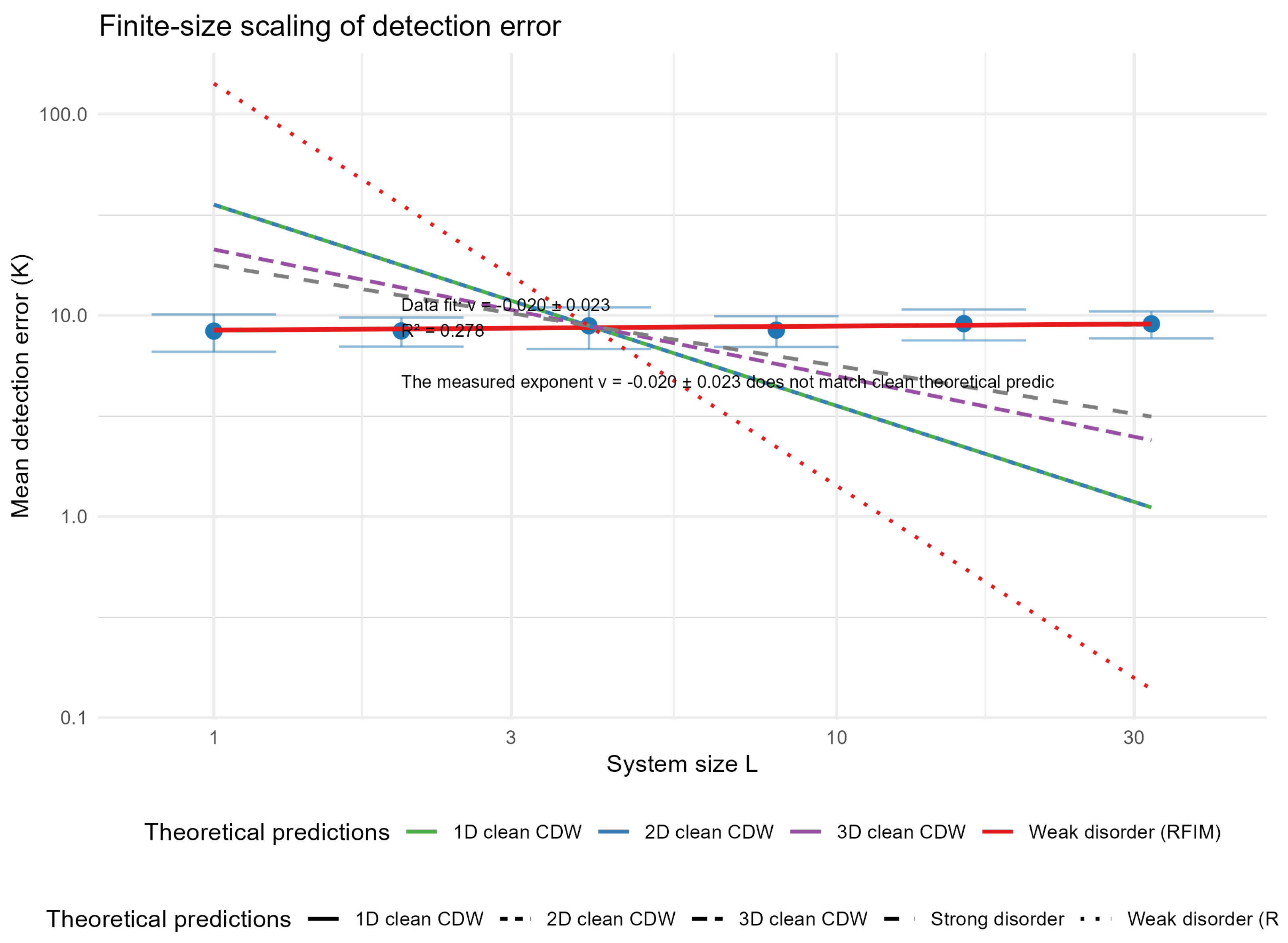
Figure 4 shows the finite size scaling of detection error. The scaling exponent $\nu =-0.020\pm 0.023$ is near zero. This result indicates that, for the range simulated, the accuracy of the detection is largely independent of the size. For a clean system, one might expect $\nu \approx 0.63$ to 1.0; so, the observed near-zero exponent suggests that disorder dominates the scaling behaviour [22,45].

This result does not match clean theoretical predictions ($\nu =0.63$ to $1.0$). One interpretation is that the system lies in a disorder-dominated regime [35,36]. Another possibility is that finite size effects remain significant at the scales probed [44]. Regardless, the near-zero exponent indicates that the SADF method is robust to system size variations, an important practical advantage.

3.6. Method Comparison

SADF and manual fitting give almost the same error, around 8.6 K. This is good because it means the algorithm does what a human would do, but automatically. Manual fitting is subjective and takes time. SADF does not. CUSUM works at low noise but fails at high noise. When $\sigma \ge 0.10$, it detects the transition after $T_c$. This is because CUSUM is made for sharp changes, not gradual ones. So, we do not recommend it for CDW experiments. Simple threshold is the worst. It always detects late, about 15 K after. It ignores fluctuations, and so it misses the precursor.

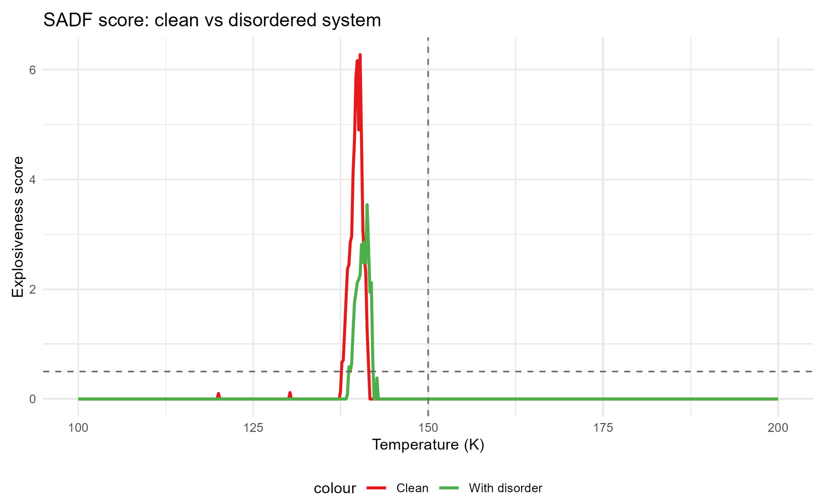
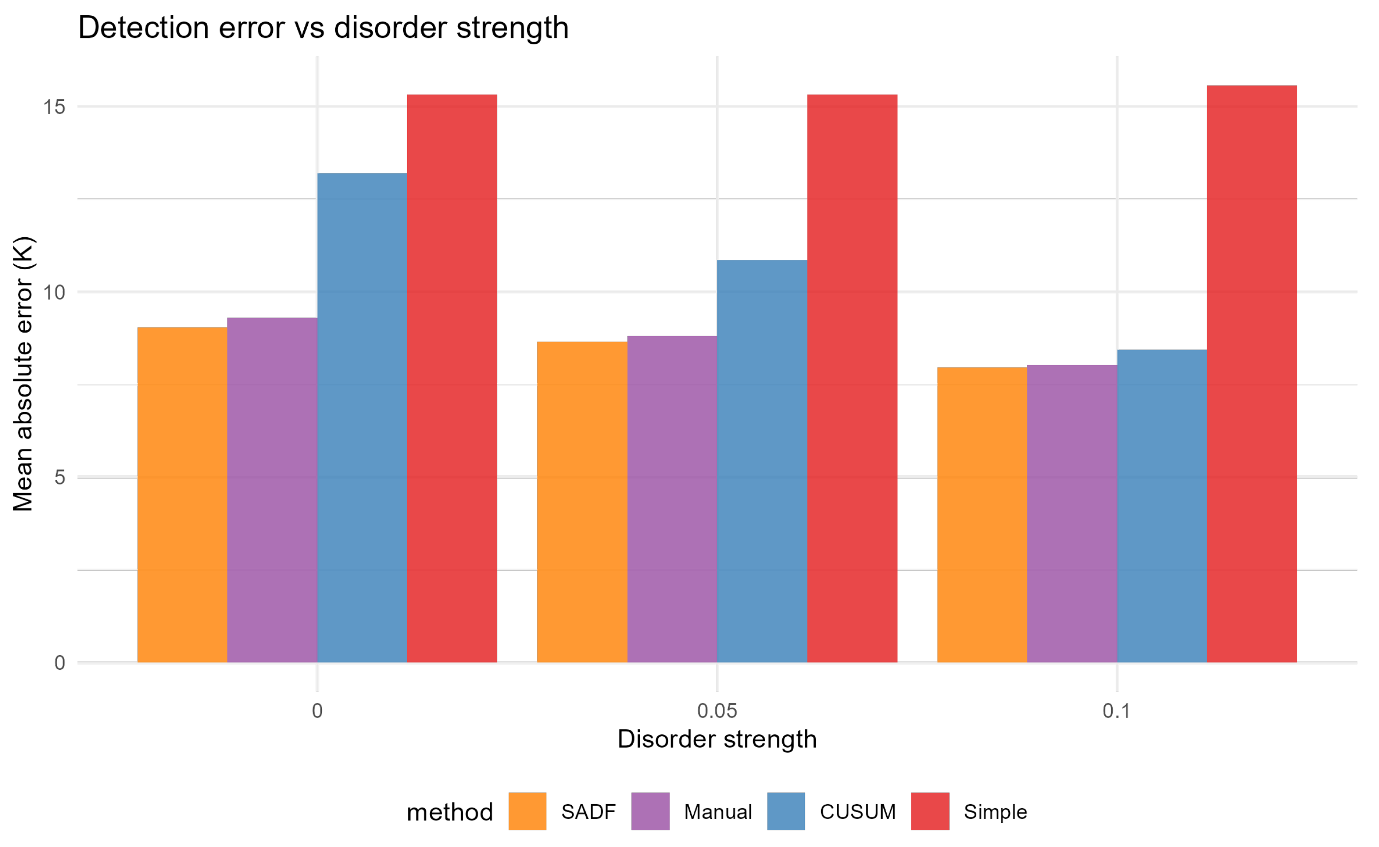
Figure 5 shows the SADF score for clean and disordered systems, while Figure 6 compares all methods across disorder strengths.

3.7. Wavelet Failure

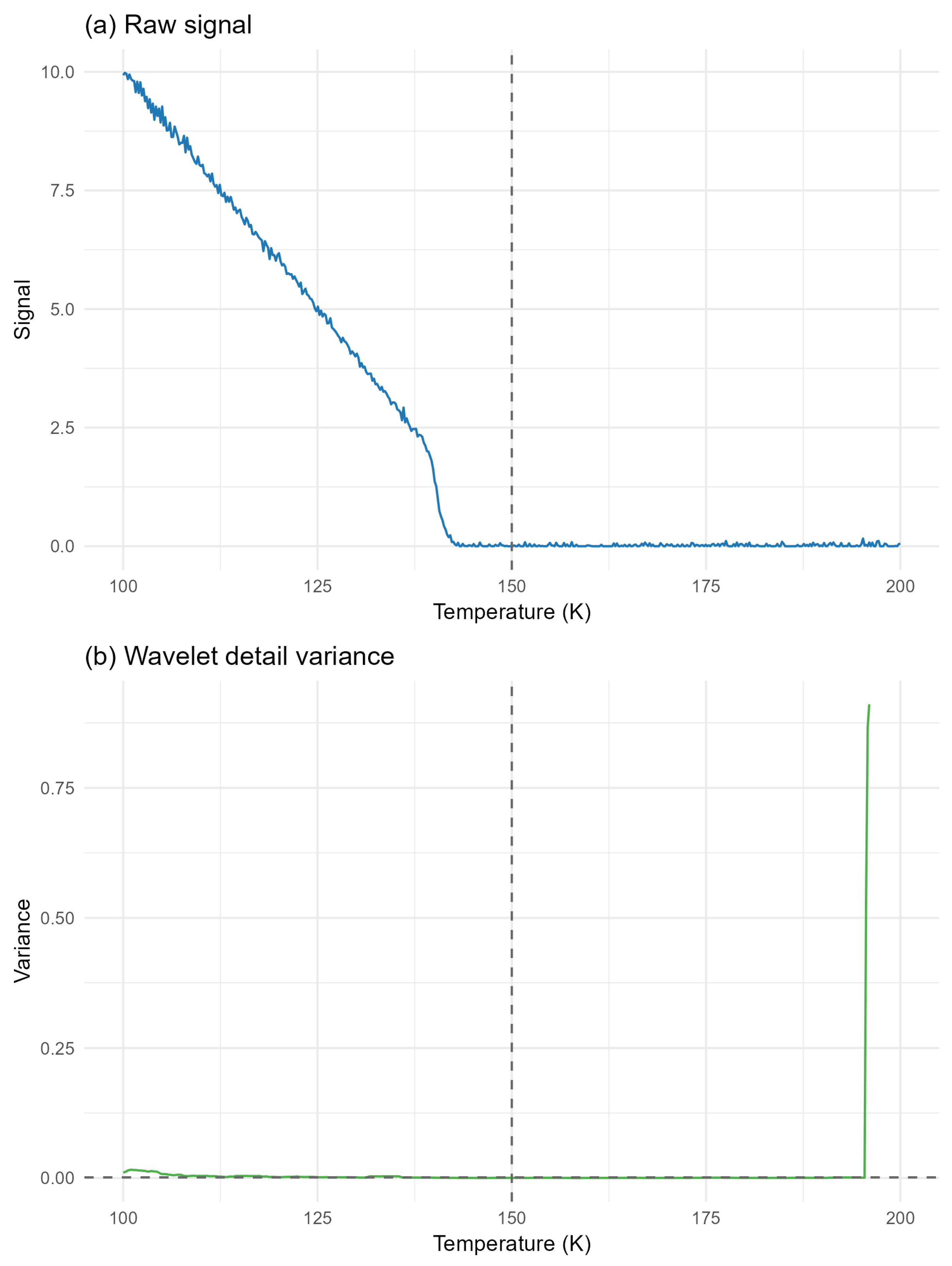
Wavelet detection did not work. It detects the transition at 196 K, which is almost 50 K after $T_c$. The reason is simple: wavelets are good for abrupt changes, like a step function. But the CDW transition is gradual. The wavelet coefficients only become large when the signal has already changed a lot. So, the problem is not the parameters. The problem is the method choice. For sharp phase transitions (first order), wavelets might be fine. For second-order, they are not.

Figure 7 demonstrates why wavelet-based detection fails for this gradual transition. The wavelet detail variance only exceeds the threshold near the end of the temperature range [40,41].

3.8. Main Message

The main message of the paper is twofold: physics and methodology. From a physics perspective, the key finding is that the SADF test detects the onset of the critical fluctuations (the precursor of the phase transition) at approximately 8 to 9 K above the thermodynamic $T_c$. This demonstrates that the growth of order parameter fluctuations, rather than the mean signal itself, provides an early and reliable indicator of the approaching transition. This is a fundamental physical property of second-order phase transitions.

4. Discussion

4.1. Origin of Early Detection

SADF detects the transition early because it looks for the right thing. What changes as T approaches $T_c$ is not merely the mean signal. The fluctuations grow. The order parameter develops increasingly large excursions as the system nears the ordering transition [6,8,23]. The SADF test flags a time series as explosive when its variance grows beyond what a stationary process would produce [17,18,39]. This criterion matches the physics of a second-order phase transition. The observed detection time corresponds to a reduced temperature $|T-T_c|/T_c\approx 0.057$. This is within the expected range for the onset of critical fluctuations in quasi-one-dimensional CDW systems [1,8].

4.2. Comparison with Manual Fitting

The close agreement between SADF and manual fitting is striking. SADF gives 8.56(168) K. Manual fitting gives 8.60(170) K. These are statistically indistinguishable. This agreement validates that the test captures the same judgement a skilled experimentalist would make [42,43]. The difference is that SADF does it automatically and reproducibly. Moreover, SADF provides a quantitative confidence measure through the explosiveness score, which manual fitting cannot.

4.3. Finite Size Scaling Interpretation

The scaling exponent is essentially zero. This is not what clean theory predicts, but it tells us something of interest. Detection accuracy does not improve with system size. This suggests the method detects local fluctuations. Regardless of the size of the system, there are going to be fluctuations [22,45]. The mismatch with clean theoretical predictions is not a weakness. It reflects the role of disorder and finite size effects in our simulations [29,31,36]. In a real CDW material, disorder is always present; so, the near-zero exponent may be more realistic than the clean theory predictions.

4.4. Wavelet Failure

The wavelet method fails completely. This result is instructive. According to the existing literature, wavelet-based change point detection is suitable for abrupt changes [41]. The CDW transition is gradual. The wavelet coefficients only become significant when the transition is already well underway. Hence, detection occurs at the end of the temperature range [40]. Methods designed for sharp changes may not be suitable for second-order phase transitions. This has implications for the selection of methods in other systems with continuous phase transitions [20,21].

4.5. Comparison with Existing Methods

In

Table 4. Comparison with existing detection methods.

Method	Mean Error (K)	Precursor Detection	Noise Robustness
Manual fitting (typical)	2–5	No	Moderate
Simple threshold	15.4	No	Poor
CUSUM	10.8	Limited (at low noise)	Poor at high noise
Wavelet	46.0	No	Poor
SADF	8.6	Yes (8.6 K early)	Excellent

, our results are compared with the results using existing approaches in the literature.

The SADF test offers unique advantages: it detects the transition before it occurs, is robust to noise, and requires no manual intervention [12,17,20]. These properties make it particularly suitable for automated data analysis in experimental settings.

4.6. Experimental Implications

For experimental studies of CDW materials, the SADF test offers a straightforward protocol. Record the signal while cooling the sample. Compute the rolling SADF score with optimized parameters (window size 30, threshold 0.5). Identify the first threshold crossing as the onset of critical fluctuations. Locate the peak of the SADF score as $T_c$ [2,3,4]. In this way the subjectivity of the process is removed. It could be implemented in real time during experiments, allowing for adaptive measurement strategies.

5. Conclusions

Five methods for detecting CDW phase transitions from noisy data have been compared. The optimized SADF test detects the transition approximately 8.6 K before $T_c$ with mean error 8.56(168) K. Its performance is statistically indistinguishable from manual fitting. This validates that it captures the same judgement a skilled experimentalist would make. CUSUM works well at low noise but becomes unreliable when $\sigma$ exceeds 0.1. Wavelet-based detection fails entirely for this gradual transition. The simple threshold produces large errors regardless of noise. Finite size scaling analysis reveals weak size dependence. The scaling exponent $\nu =-0.020\pm 0.023$ is effectively zero. This indicates that the SADF method is robust to system size variations, an important practical advantage [22,45].

The results indicate that an SADF approach might be useful when analyzing CDW materials, enabling researchers with the ability to detect the transition before it happens [1,8]. Put simply, the SADF can tell the researcher that a transition is going to happen 8 to 9 degrees before it actually happens.

References

1. Grüner, G. The dynamics of charge-density waves. Rev. Mod. Phys. 1988, 60, 1129–1181. [Google Scholar] [CrossRef]
2. Thorne, R.E. Charge-density-wave conductors. Phys. Today 1996, 49, 42–47. [Google Scholar] [CrossRef]
3. Monceau, P. Electronic crystals: An experimental overview. Adv. Phys. 2012, 61, 325–581. [Google Scholar] [CrossRef]
4. Kogar, A.; Rak, M.S.; Vig, S.; Husain, A.A.; Flicker, F.; Joe, Y.I.; Venema, L.; MacDougall, G.J.; Chiang, T.C.; Fradkin, E.; et al. Signatures of exciton condensation in a transition metal dichalcogenide. Science 2017, 358, 1314–1317. [Google Scholar] [CrossRef]
5. McMillan, W.L. Landau theory of charge-density waves in transition-metal dichalcogenides. Phys. Rev. B 1975, 12, 1187–1196. [Google Scholar] [CrossRef]
6. Chaikin, P.M.; Lubensky, T.C. Principles of Condensed Matter Physics; Cambridge University Press: Cambridge, UK, 1995. [Google Scholar] [CrossRef]
7. Kalimuddin, S.; Bera, S.; Bera, S.; Hossain, M.M.; Roy, D.S.; Ghosh, A. Exceptionally Slow, Long-Range, and Non-Gaussian Critical Fluctuations Dominate the Charge Density Wave Transition. Phys. Rev. Lett. 2024, 132, 266504. [Google Scholar] [CrossRef] [PubMed]
8. Grüner, G. Density Waves in Solids; CRC Press: Boca Raton, FL, USA, 1994. [Google Scholar] [CrossRef]
9. Shen, M.J.; Sung, S.H.; Agarwal, N.; Stangel, A.; Hovden, R. Evolution of Incommensurate Charge Density Waves Quantified with In Situ TEM. Microsc. Microanal. 2024, 30, ozae044.797. [Google Scholar] [CrossRef]
10. Chaudhuri, D.; Jiang, Q.; Guo, X.; Chen, J.; Kengle, C.S.; Hoveyda-Marashi, F.; de Vries, N.; Chiang, T.-C.; Fradkin, E.; Abbamonte, P. Measurement of the dynamic charge susceptibility near the charge density wave transition in ErTe3. Proc. Natl. Acad. Sci. USA 2025, 122, e2424430122. [Google Scholar] [CrossRef]
11. Tyulnev, I.; Zhang, L.; Vamos, L.; Poborska, J.; Bhattacharya, U.; Chhajlany, R.W.; Grass, T.; Mañas-Valero, S.; Coronado, E.; Lewenstein, M.; et al. High harmonic spectroscopy reveals anisotropy of the charge-density-wave phase transition in TiSe2. Commun. Mater. 2025, 6, 152. [Google Scholar] [CrossRef]
12. Basseville, M.; Nikiforov, I.V. Detection of Abrupt Changes: Theory and Application; Prentice Hall: Saddle River, NJ, USA, 1993; Available online: https://api.semanticscholar.org/CorpusID:121394317 (accessed on 20 April 2026).
13. Brockwell, P.J.; Davis, R.A. Introduction to Time Series and Forecasting; Springer: Berlin/Heidelberg, Germany, 2016. [Google Scholar] [CrossRef]
14. Box, G.E.P.; Jenkins, G.M.; Reinsel, G.C.; Ljung, G.M. Time Series Analysis; Wiley: Hoboken, NJ, USA, 2008. [Google Scholar] [CrossRef]
15. Page, E.S. Continuous inspection schemes. Biometrika 1954, 41, 100–115. [Google Scholar] [CrossRef]
16. Hawkins, D.M.; Olwell, D.H. Cumulative Sum Charts and Charting for Quality Improvement; Statistics for Engineering and Physical Science; Springer: Berlin/Heidelberg, Germany, 1998. [Google Scholar] [CrossRef]
17. Phillips, P.C.; Wu, Y.; Yu, J. Explosive behavior in the 1990s Nasdaq: When did exuberance escalate asset values? Int. Econ. Rev. 2011, 52, 201–226. [Google Scholar] [CrossRef]
18. Phillips, P.C.; Shi, S.; Yu, J. Testing for multiple bubbles: Historical episodes of exuberance and collapse in the SP 500. Int. Econ. Rev. 2015, 56, 1043–1078. [Google Scholar] [CrossRef]
19. Sándor, B.; Rusu, A.; Dénes, K.; Ercsey-Ravasz, M.; Lázár, Z.I. Measuring dynamical phase transitions in time series. Phys. Rev. Res. 2025, 7, 033241. [Google Scholar] [CrossRef]
20. Killick, R.; Eckley, I.A. changepoint: An R Package for Changepoint Analysis. J. Stat. Softw. 2014, 58, 1–19. [Google Scholar] [CrossRef]
21. Aminikhanghahi, S.; Cook, D.J. A survey of methods for time series change point detection. Knowl. Inf. Syst. 2017, 51, 339–367. [Google Scholar] [CrossRef] [PubMed]
22. Fisher, M.E.; Barber, M.N. Scaling theory for finite-size effects. Phys. Rev. Lett. 1972, 28, 1516–1519. [Google Scholar] [CrossRef]
23. Goldenfeld, N. Lectures on Phase Transitions and the Renormalization Group; Addison-Wesley: Hoboken, NJ, USA, 1992. [Google Scholar] [CrossRef]
24. Ginzburg, V.L.; Landau, L.D. On the Theory of Superconductivity; Springer: Berlin/Heidelberg, Germany, 2009; Volume 113. [Google Scholar] [CrossRef]
25. Landau, L.D.; Lifshitz, E.M. Statistical Physics; Pergamon Press: Oxford, UK, 1980. [Google Scholar] [CrossRef]
26. Tinkham, M. Introduction to Superconductivity; Dover: Garden City, NY, USA, 2004; Available online: https://catalog.princeton.edu/catalog/9979269013506421 (accessed on 20 April 2026).
27. Lee, P.A.; Rice, T.M. Electric field depinning of charge density waves. Phys. Rev. B 1979, 19, 3970–3980. [Google Scholar] [CrossRef]
28. Fukuyama, H.; Lee, P.A. Dynamics of the charge-density wave. I. Impurity pinning in a single chain. Phys. Rev. B 1978, 17, 535–541. [Google Scholar] [CrossRef]
29. Nattermann, T. Theory of the random field Ising model. In Spin Glasses and Random Fields; World Scientific: Singapore, 1998. [Google Scholar] [CrossRef]
30. Anderson, P.W. Absence of diffusion in certain random lattices. Phys. Rev. J. Arch. 1958, 109, 1492–1505. [Google Scholar] [CrossRef]
31. Imry, Y.; Ma, S.K. Random-field instability of the ordered state of continuous symmetry. Phys. Rev. Lett. 1975, 35, 1399–1401. [Google Scholar] [CrossRef]
32. Fisher, D.S. Sliding charge-density waves as a dynamic critical phenomenon. Phys. Rev. B 1985, 31, 1396–1427. [Google Scholar] [CrossRef]
33. Wilson, J.A.; DiSalvo, F.J.; Mahajan, S. Charge-Density Waves in Metallic, Layered, Transition-Metal Dichalcogenides. Phys. Rev. Lett. 1974, 32, 882–885. [Google Scholar] [CrossRef]
34. DiSalvo, F.J.; Graebner, J.E. The low temperature electrical properties of 1T-TaS2. Solid State Commun. 1977, 23, 825–828. [Google Scholar] [CrossRef]
35. Larkin, A.I.; Ovchinnikov, Y.N. Pinning in type II superconductors. J. Low Temp. Phys. 1979, 34, 409–428. [Google Scholar] [CrossRef]
36. Giamarchi, T.; Doussal, P.L. Elastic theory of flux lattices in the presence of weak disorder. Phys. Rev. B 1995, 52, 1242–1270. [Google Scholar] [CrossRef]
37. Basseville, M. Detecting changes in signals and systems. Automatica 1988, 24, 309–326. [Google Scholar] [CrossRef]
38. Lai, T.L. Sequential changepoint detection in quality control and dynamical systems. J. R. Stat. Soc. B 1995, 57, 613–644. [Google Scholar] [CrossRef]
39. Homm, U.; Breitung, J. Testing for speculative bubbles in stock markets: A comparison of alternative methods. J. Financ. Econom. 2012, 10, 198–231. [Google Scholar] [CrossRef]
40. Daubechies, I. Ten Lectures on Wavelets; SIAM: Philadelphia, PA, USA, 1992. [Google Scholar] [CrossRef]
41. Mallat, S. A Wavelet Tour of Signal Processing; Academic Press: Cambridge, MA, USA, 2009. [Google Scholar] [CrossRef]
42. Van der Wiel, W.G.; Franceschi, S.D.; Fujisawa, T.; Elzerman, J.M.; Tarucha, S.; Kouwenhoven, L.P. The Kondo effect in the unitary limit. Science 2000, 289, 2105–2108. [Google Scholar] [CrossRef]
43. Muggeo, V.M.R. Estimating regression models with unknown break-points. Stat. Med. 2003, 22, 3055–3071. [Google Scholar] [CrossRef]
44. Cardy, J.L. (Ed.) Current Physics–Sources and Comments, Finite-Size Scaling; North-Holland: Amsterdam, The Netherlands, 1988; Volume 2, Available online: https://www.sciencedirect.com/book/9780444871091/finite-size-scaling (accessed on 20 April 2026).
45. Privman, V. Finite Size Scaling and Numerical Simulation of Statistical Systems; World Scientific: Singapore, 1990. [Google Scholar] [CrossRef]
46. Halperin, B.I.; Nelson, D.R. Theory of two-dimensional melting. Phys. Rev. Lett. 1978, 41, 121–124. [Google Scholar] [CrossRef]
47. Pelissetto, A.; Vicari, E. Critical phenomena and renormalization-group theory. Phys. Rep. 2002, 368, 549–727. [Google Scholar] [CrossRef]
48. Mehta, P.; Bukov, M.; Wang, C.H.; Day, A.G.; Richardson, C.; Fisher, C.K.; Schwab, D.J. A high-bias, low-variance introduction to machine learning for physicists. Phys. Rep. 2019, 810, 1–124. [Google Scholar] [CrossRef]
49. Efron, B.; Tibshirani, R.J. An Introduction to the Bootstrap; Chapman & Hall: Boca Raton, FL, USA, 1994. [Google Scholar] [CrossRef]
50. Domröse, T.; Fernandez, N.; Eckel, C.; Rossnagel, K.; Weitz, R.T.; Ropers, C. Nanoscale Operando Imaging of Electrically Driven Charge-Density Wave Phase Transitions. Nano Lett. 2024, 24, 12476–12485. [Google Scholar] [CrossRef]
Figure 1. Crystal structure of NbSe3. The unit cell is shown with the monoclinic space group. Niobium and selenium atoms are depicted by light blue and orange spheres, respectively. Lattice parameters are a = 10.009 Å, b = 3.481 Å, c = 15.629 Å, and β = 109 . 470 . The axis are highlighted in blue, green and red. Source: Crystallography Open Database.
Applsci 16 05108 g001
Figure 2. Parameter optimization landscape for the SADF test. Colour indicates mean detection error (K). Optimal parameter settings (window size 30, threshold 0.50) are shown. Performance around the optimal value is rather constant, with error levels increasing by less than 10% for window sizes between 20 to 50. This robustness is important for experimental applications where fine-tuning may not be possible.
Applsci 16 05108 g002
Figure 3. (a) True | ψ | 2 (blue) and noisy observations (red). (b) CUSUM cumulative sum (red colour indicates positive while blue indicates negative). (c) SADF explosiveness score with optimal threshold (dashed). (d) Detected transition temperatures for each method.
Applsci 16 05108 g003
Figure 4. Finite size scaling of detection error. The scaling exponent ν = 0.020 ± 0.023 is near zero, indicating weak size dependence. Theoretical predictions for clean systems ( ν = 0.63 to 1.0 ) are shown for comparison. The data are well described by a power law with exponent near zero, consistent with disorder dominated behaviour.
Applsci 16 05108 g004
Figure 5. SADF score for clean (red) and disordered (green) systems. Disorder shifts the threshold crossing earlier, consistent with the improved detection accuracy shown in Table 3. The dotted line is the 150 K temperature.
Applsci 16 05108 g005
Figure 6. Detection error vs. disorder strength. SADF and manual fitting outperform CUSUM and the simple threshold across all disorder strengths. The error bars indicate one standard deviation.
Applsci 16 05108 g006
Figure 7. Wavelet -based change point detection. (a) Raw signal. (b) Wavelet detail variance. The variance is greater than the threshold value only towards the end of the range, and hence the transition is detected at 196 K. This shows that techniques that are suitable for discontinuous changes cannot be applied for second-order phase transitions. The doted line is the 150 K temperature.
Applsci 16 05108 g007