Dotsformer: Capturing Chain-Loop Structures for Transformer in Dots-and-Boxes

Abstract

In many board games, AlphaZero has demonstrated superhuman abilities. Dots-and-Boxes is a classic board game with simple rules but requiring skills to win. This paper proposes Dotsformer, which extracts chain-loop structures from the game board. These structures connect distant boxes, providing long-range relational information as input to the Transformer. We employ multiple convolutional kernels to generate Q, K, and V, and incorporate information about the box structure itself into the attention scores. We also incorporate auxiliary training tasks, including an initiative task and a classification task. These tasks determine whether to retain or relinquish the initiative in the current situation, and classify actions into forbidden, conceding, safe, and scoring moves. They provide additional supervisory signals and accelerate learning. The experimental results show that Dotsformer outperforms AlphaZero in both rollback speed and playing strength: it achieved a winning rate of 87.6% and an ELO rating lead of 340 points against the baseline. Additionally, ablation studies verify the effectiveness of each key module.

1. Introduction

For millennia, board games have stood as one of the most popular and elegant intellectual pursuits unique to humans. This is owing to their simple and transparent rules. Their challenge lies in whether a player can rely on strategic and computational foresight to identify superior strategies. These strategies are ones capable of anticipating multiple moves ahead. All of this must be done within the combinatorial explosion of state and strategy space. Since the term “artificial intelligence” was coined in 1956, board games have served as both the “Drosophila” of machine intelligence research and a touchstone for evaluating machine learning algorithms. In 2016, AlphaGo [1], developed by Google DeepMind, decisively defeated the world champion Lee Sedol in a widely publicized Go match. This milestone demonstrated that mastering board games is no longer the exclusive glory of humans. Artificial agents can not only master them but also surpass human capabilities. Methodologically, deep reinforcement learning has become the state-of-the-art approach for the study of board games.

Subsequently, a sequence of more powerful deep reinforcement learning algorithms, including AlphaGo Zero [2], AlphaZero [3], MuZero [4], and KataGo [5,6], was proposed. These algorithms achieved superhuman performance in various complex games through self-play, including chess [7], Go [2], Shogi [3], and even Mahjong [8]. Their advantages are numerous. They do not require human expert knowledge, and they effectively utilize the self-supervised policy improvement of MCTS [9]. In addition, they leverage the powerful approximation of deep neural networks that serve simultaneously as value and policy functions. They can also learn sophisticated decision-making without explicit access to game rules [4].

Despite these advances, the neural network architectures used in most contemporary deep reinforcement learning methods remain relatively primitive. Leading model variants remain largely bound to residual convolutional neural networks (residual CNNs). In contrast, the Transformer [10] architecture, which was introduced as early as 2017, has revolutionized temporal and spatial modeling paradigms. It has demonstrated remarkable versatility across multiple fields, including natural language processing [11,12,13], computer vision [14,15,16], and multi-modal learning [17,18,19]. More recently, LLMs (e.g., GPT-3 [20], GPT-4 [21], DeepSeek [22], PaLM [23], LLaMA [24]) have made notable progress in reasoning efficiency and multi-modal capabilities, opening up new possibilities for multi-task and generative applications. Board game play inherently possesses both linguistic and visual characteristics. The progression of a game forms a temporal sequence analogous to natural language. Meanwhile, a board state constitutes spatial data akin to an image.

Numerous research studies of AI for board games have attempted to apply Transformers to policy learning and board state evaluation. Established CNN-based architectures, such as ResNet [25], GoogLeNet [26], and DenseNet [27], have been widely used in this field. However, applying Transformers here faces a distinct challenge: finding a representation scheme that balances spatial and temporal characteristics. One common approach is to feed raw sequences of board state into residual CNNs with fixed temporal windows. Yet, residual CNNs alone are inefficient at capturing temporal and spatial dependencies. Alternatively, replacing residual CNNs with the Transformer architecture raises the question of how Transformers can process 2-dimensional board data and understand the rules of the game. There is no obvious, generally applicable method.

In Dots-and-Boxes [28], a move affects not only the current box’s score but also the potential formation of chains and loops. Opening such structures prematurely allows the opponent to score consecutively. Therefore, capturing the chain-loop structure on the board is crucial. While traditional residual CNNs struggle to capture such long-range dependencies, Transformers are inherently well-suited for this task. However, applying existing approaches to the dynamic chain-like structures of Dots-and-Boxes reveals limitations. Many methods fail to explicitly capture the underlying chain topology in their board representations. At the architectural level, it remains difficult to preserve local details while effectively integrating global information. In addition, conventional policy–value heads are not well-suited to model initiative, which plays an important role in describing advantage transitions during gameplay.

To address these issues, we propose Dotsformer, a hybrid architecture that integrates Transformers with residual CNNs. This design enables the model to simultaneously extract chain-loop features, attend to local regions of the board, and capture connections between distant boxes. The key contributions of this paper are as follows:

• ChainLoop6: We propose the ChainLoop structure-aware representation. It explicitly encodes chain and loop structures on the board. This overcomes the limitations of traditional coordinate encoding, which struggles to capture topological relationships.
• MS-Trans: We design the MS-Trans architecture. It incorporates topological structural bias into the Transformer attention mechanism, enhancing the model’s ability to capture long-range structural dependencies.
• Auxiliary Tasks Learning: We introduce auxiliary tasks. By leveraging multi-task learning, it improves feature representation and boosts training efficiency. Specifically, the model predicts whether the next move is a capture, sacrifice, or neutral action, while classifying all potential moves on the board as forbidden, conceding, safe, or scoring.
• Dotsformer: We systematically integrate Transformer, auxiliary tasks, self-play reinforcement learning, and Monte Carlo tree search into a unified framework. This establishes a complete training and evaluation pipeline for Dots and Boxes. Comprehensive experiments validate the effectiveness of our approach.

The remainder of this paper is organized as follows. In Section 2, we review the related work. In Section 3, we introduce the basic rules of Dots-and-Boxes. In Section 4, we present the main methodology adopted in this paper. In Section 5, we conduct extensive experiments to demonstrate the effectiveness and superiority of Dotsformer.

2. Related Work

2.1. Search Algorithms

Nascent theoretical foundations were established by von Neumann (1928) with the Minimax Theorem [29], which provided the mathematical basis for two-player zero-sum games. Claude Shannon (1950) was among the first to apply Minimax [30] search to chess. He proposed depth-limited game trees combined with heuristic evaluation functions. However, the exponential growth of the game tree rendered exhaustive search computationally intractable, motivating the need for algorithmic optimizations.

Zobrist (1970) [31] introduced transposition tables, which reduce redundant computations by caching previously encountered board states. Knuth and Moore (1975) [32] later provided a rigorous mathematical analysis of the Alpha-Beta pruning algorithm. This work showed that pruning irrelevant branches can increase the effective search depth. Despite these major improvements in search efficiency, the decision quality still depended heavily on handcrafted heuristics.

Subsequently, Iterative Deepening Search (Korf, 1985) [33] combined the advantages of depth-first and breadth-first search to efficiently exploit principal variations. This line of classical search techniques culminated in 1997, when IBM’s Deep Blue defeated the world chess champion, Kasparov. The architecture and strategies of Deep Blue were later analyzed in detail by Campbell et al. [34]. To address games with high branching factors (e.g., Go), Monte Carlo Tree Search (MCTS) became the dominant approach. Specifically, the UCT algorithm [35] (Kocsis & Szepesvári, 2006) achieved a balance between exploration and exploitation through statistical sampling.

2.2. Network Architectures

Early computer board game systems relied primarily on hand-crafted features and heuristic search algorithms. AlphaGo [1] introduced convolutional neural networks (CNNs) together with supervised learning to effectively guide MCTS. Subsequently, AlphaZero [3] incorporated ResNet [25] and discarded human prior knowledge, achieving generic superhuman performance across multiple board games through pure self-play reinforcement learning.

In recent years, following the success of the Transformer architecture in reinforcement learning [36], researchers have begun exploring its application in board game decision-making tasks. The application of Transformers in board games can be broadly categorized into two directions. One treats game playing as a generative task, where decisions are produced through sequence modeling. The other leverages the attention mechanism as a replacement for conventional convolutional neural networks, aiming to improve playing strength by capturing global dependencies more effectively.

In the sequence modeling paradigm, researchers moved away from explicit search procedures and instead modeled game play as an autoregressive sequence prediction problem. Game records were reformulated as token sequences, and subsequent moves were generated by predicting the next token using language models. This paradigm was explored by Ciolino et al. [37], who fine-tuned GPT-2 on Go game records to predict moves as next-token tasks. Subsequent work extended this approach: Othello-GPT [38] demonstrated that transformers learn interpretable board-state representations, while ChessGPT [39] incorporated natural language data to generate move explanations alongside predictions. Despite these advantages, sequence modeling approaches remained limited by their reliance on imitation learning and the absence of explicit search. As a result, they often struggled with long-term strategic reasoning and generalization beyond the training distribution.

From the perspective of network architecture, Transformers were explored as either a substitute for or a complement to convolutional backbones. In this direction, Sagri et al. [40] explored Vision Transformer backbones within a KataGo-style framework. Other work focused on architectural adaptations: Chessformer [41] introduced structure-aware positional encoding, while ResTNet [42] combined residual and Transformer blocks in a hybrid design. Overall, Transformer-based models improve global dependency modeling, while hybrid designs aim to balance global context with local inductive biases.

Beyond attention-based approaches, graph neural networks (GNNs) were also explored for board games. Keller et al. [43] showed that GNNs were effective at modeling long-range dependencies in Hex, but also showed reduced proficiency in discerning local patterns. Rigaux and Kashima [44] proposed a graph-based representation for chess, reporting improved playing strength. These results suggested that GNNs provide a flexible way to encode relational structures, but may struggle to efficiently capture local patterns and face computational constraints.

To provide a systematic overview of existing approaches and highlight the novelty of our work, we summarize prior studies in

Table 1. Comparison of our proposed approach with existing methods.

Model	State Encoding	Architecture	Search	Supervision	Output	Game
AlphaGo [1]	Grid	CNN	MCTS	SL + RL	PH, VH	Go
AlphaGo Zero [2]	Grid	ResNet	MCTS	RL	PH, VH	Go
AlphaZero [3]	Grid	ResNet	MCTS	RL	PH, VH	Chess, Go, Shogi
Go Transformer [37]	Sequence	Causal Trans.	None	SL	LM Head	Go
Othello-GPT [38]	Sequence	Causal Trans.	None	SL	LM Head	Othello
ChessGPT [39]	Sequence	Causal Trans.	None	SL	LM Head	Chess
EfficientFormer [40]	Grid	Vision Trans.	MCTS	SL	PH, VH	Go
Chessformer [41]	Sequence	Transformer	None	SL	Multi PHs/VHs *	Chess
Tjong [8]	Grid	TIT	None	SL + RL	Hierarchical PH, VH	Mahjong
ResTNet [42]	Grid	ResNet + Trans.	MCTS	RL/SL	PH, VH	Go, Hex
GraphDQN [43]	Graph	GNN	None	RL	Q-values	Hex
GraphAra [43]	Graph	GNN	MCTS	SL + RL	PH, VH	Hex
AlphaGateau [44]	Graph	GNN	MCTS	RL	PH, VH	Chess
Dotsformer (Ours)	Grid + ChainLoop	MS-Trans	MCTS	RL	PH, VH, Init., Class.	Dots-and-Boxes

Note: PH: Policy Head, VH: Value Head, LM Head: Language Modeling Head. * Chessformer uses multiple auxiliary PHs and VHs. RL/SL: RL (9 × 9 Go, 19 × 19 Hex), SL (19 × 19 Go). Init.: Initiative Head, Class.: Classification Head.

across six key dimensions: state encoding, architecture, search role, supervision type, output, and game.

3. Rules of Dots-and-Boxes and Notations

3.1. Rules of Dots-and-Boxes

Players take turns drawing horizontal or vertical edges between adjacent dots. Each edge can be drawn only once. Completing a $1\times 1$ box grants one point and an immediate extra turn, which often leads to consecutive scoring. A single move can impact the initiative (defined as the ability to retain or relinquish control over turn continuation by deciding whether to claim available boxes) across the entire board. As the game proceeds, complex chain and loop structures emerge, making the control of initiative the primary strategic element rather than just box counting. The game concludes once all edges are drawn, with the highest score winning.

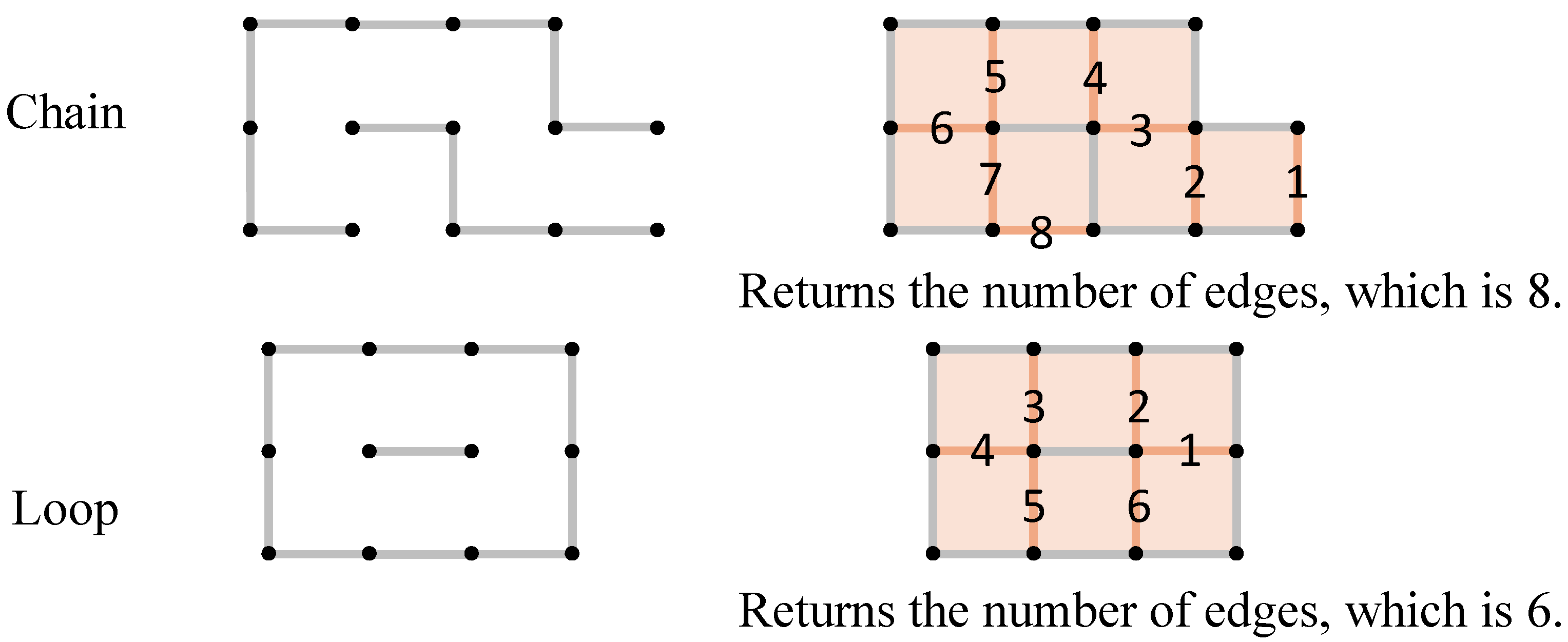
The following example illustrates these chain and loop structures and demonstrates the edge counts returned by the Chain-Loop Detection, as shown in Figure 1.

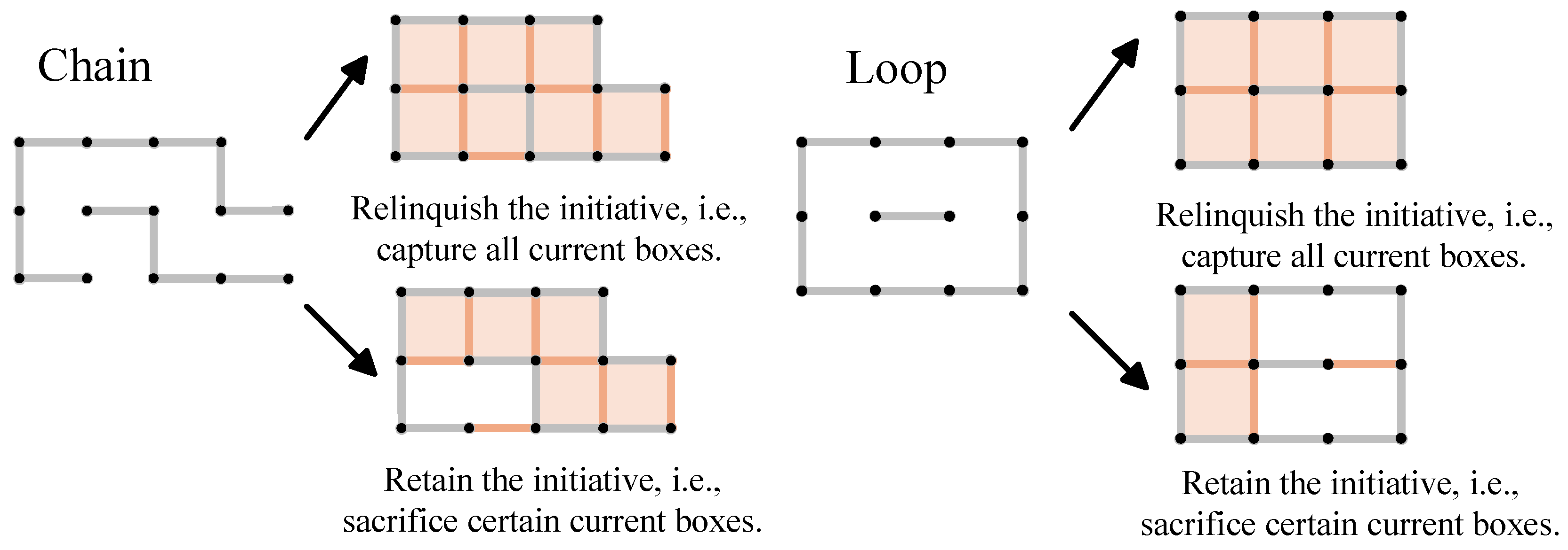
Since completing a box grants an extra move, initiative plays a central role in Dots-and-Boxes. Players must carefully consider the relationship between immediate scoring opportunities and initiative. In particular, careless local scoring can result in a loss of initiative around chain and loop structures during critical stages of the game. Figure 2 provides a schematic illustration of initiative.

3.2. Notations

To ensure consistent notation throughout the paper, we compile the main symbols in

Table 2. Summary of key notations.

Notation	Description
X	Input tensor
N	Board length: 5
C	Number of channels of the input tensor
D	Input channels, set to 128
$x_{ij}$	The feature vector at coordinate $(i,j)$
$e_{ij}^k$	The vector at coordinate $(i,j)$ in channel k, for dots or edges
m	(Red boxes count − Blue boxes count) $\times 0.25$
$c{l}_{ij}^l$	The vector at coordinate $(i,j)$ in channel l, for chain-loop representation
$e{q}_{ij}^k$	States of the four edges (right, up, left, down) in a box
$g_{ij}$	5-dimensional one-hot vector representing the number of occupied edges in a box
$d_{ij}^v$	5-dimensional one-hot vector for occupied edges of all adjacent neighbor boxes
$F_a$	Feature embedding function
$t_{ij}$	Vector input to the neural network
L	Sequence length after mapping the original $5\times 5$ board to $11\times 11$, $L=121$
B	Batch size
h	Number of attention heads, set to 4
$d_h$	Feature dimension of a single attention head
I	3-dimensional one-hot vector to indicate the current initiative
$cls$	4-way categorical vector to classify the move

.

4. Methodology

4.1. EdgeQuad and ChainLoop: Feature Representations for Dots-and-Boxes

Both local geometric and global topological features play a critical role in Dots-and-Boxes. Capturing individual boxes affects immediate scoring, while identifying chains and loops largely determines the final outcome of the game. Since the board representation is directly used as input to the neural network, we design five board feature representations to examine how different forms of input influence learning. These representations can be divided into two categories. The EdgeQuad series consists of three geometric representations that emphasize the spatial relationships between edges and boxes. They encode the raw board state by describing the distribution of edges within each box, as well as the number of edges surrounding a box. The ChainLoop series, in contrast, focuses on long-range structures by introducing additional channels that encode chain and loop membership for each edge.

Across all configurations, we represent the input to the $N\times N$ board (where $N=5$) as a spatial tensor $X\in {\mathbb{R}}^{(2N+1)\times (2N+1)\times C}$. Every model shares a core foundational structure for the first four channels ($c\in \{0,1,2,3\}$), defined as follows:

• Channel 0: Dot and box-center locations are indicated by setting the corresponding coordinates to 1, with all other positions set to 0.
• Channel 1: All horizontal and vertical edge locations are set to 1 to specify the valid action space.
• Channel 2: Edges currently occupied by a player are assigned a value of 1, while unoccupied edges remain 0.
• Channel 3: A scalar map encoding the current score differential.

$$\left\{\begin{array}{c}X\in {\mathbb{R}}^{(2N+1)\times (2N+1)\times C},\hfill \\ t_{ij}=F_a\left(x_{ij}\right),F_a:{\mathbb{R}}^C\to {\mathbb{R}}^D.\hfill \end{array}\right.$$

(1)

From this shared foundation, we evaluate three architectural variations:

Baseline: ($C=4$, $a=0$)

The baseline model relies exclusively on the four fundamental channels.

$$x_{ij}=\left(e_{ij}^0,e_{ij}^1,e_{ij}^2,m\right)\in {\mathbb{R}}^C,e_{ij}^k\in \{0,1\},k\in \{0,1,2\},m\in \mathbb{R}.$$

(2)

ChainLoop64: ($C=64$, $a=1$)

Given that a standard $5\times 5$ board contains 60 edges, we set $C=64$ to allow sufficient capacity for representing multiple chains and loops. Channels 4 through 63 each encode a single detected chain or loop, with constituent edges marked as 1 and all others 0.

$$x_{ij}=\left(e_{ij}^0,e_{ij}^1,e_{ij}^2,m,d_{ij}^4,\dots ,d_{ij}^{63}\right)\in {\mathbb{R}}^C,d_{ij}^l\in \{0,1\},l\in \{4,5,\dots ,63\}.$$

(3)

ChainLoop6: ($C=6$, $a=2$)

Assigning a separate channel to each of up to 60 independent structures is computationally inefficient. We therefore reduce the channel depth to $C=6$ (as shown in Figure 3) by summarizing the chain and loop data:

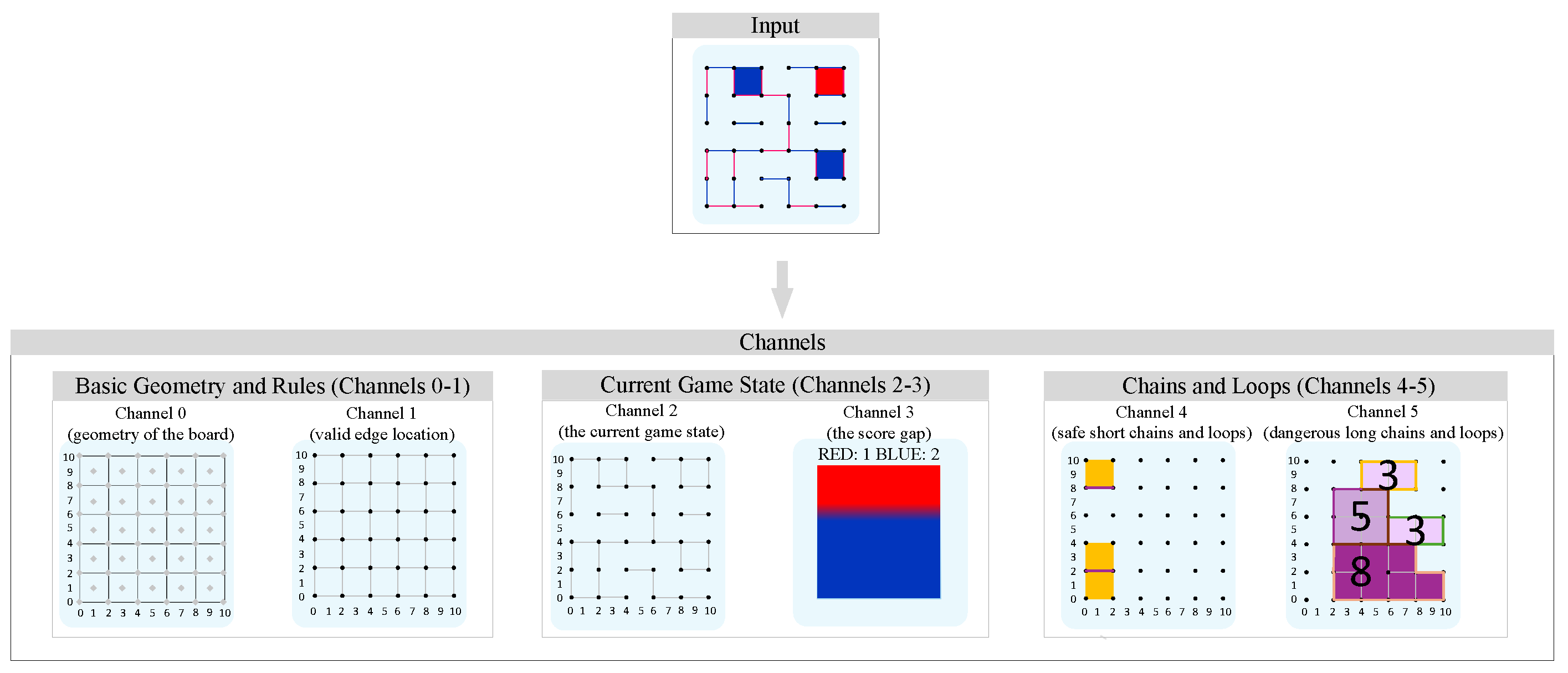
• Channel 4: Edges with a returned count of 1 from the Chain-Loop Detection, and with at least one adjacent box containing three occupied edges, are set to 1. These edges correspond to short chains that can be resolved immediately without giving the opponent control of the board.
• Channel 5: For returned edges with a length greater than 2, we set their values to the length itself. Chains or loops longer than 2 can affect the initiative in the game, and longer chains or loops correspond to a higher value.

$$x_{ij}=\left(e_{ij}^0,e_{ij}^1,e_{ij}^2,m,d_{ij}^4,d_{ij}^5\right)\in {\mathbb{R}}^C,d_{ij}^l\in \mathbb{R},l\in \{4,5\}.$$

(4)

Chain-Loop Detection:

The algorithm searches for unvisited edges and recursively checks neighboring boxes. If a box has exactly two occupied edges, the search continues. Finally, all discovered edges are combined to form chains or loops.

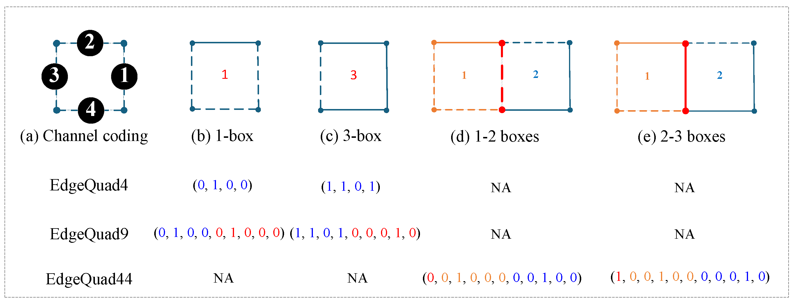
Detailed descriptions of EdgeQuad4, EdgeQuad9, and EdgeQuad44 are given in Appendix A.

Figure 3. Visualization of the six-channel feature representation for a $5\times 5$ Dots-and-Boxes game state. Channels 0 to 3 depict fundamental board information, and Channel 3 shows the Blue player’s territorial advantage, which occupies approximately two-thirds of the board. Channels 4 and 5 present the output of the Chain-Loop Detection. Channel 4 extracts chain-loop structures with a length of 1, while Channel 5 encodes chain-loop structures with a length greater than 2. The highlighted regions in Channel 5 correspond to four distinct structures, with edge counts of 3, 3, 5, and 8 returned by the Chain-Loop Detection. Figure 1 provides an explanatory visualization of the edge counts displayed in Channel 5. In Channel 3, red indicates that the red side’s territory accounts for 1/3 of the total territory, and blue indicates that the blue side’s territory accounts for 2/3 of the total territory. In Channels 4 and 5, colors are used solely for differentiation and have no special meaning.

Figure 3. Visualization of the six-channel feature representation for a $5\times 5$ Dots-and-Boxes game state. Channels 0 to 3 depict fundamental board information, and Channel 3 shows the Blue player’s territorial advantage, which occupies approximately two-thirds of the board. Channels 4 and 5 present the output of the Chain-Loop Detection. Channel 4 extracts chain-loop structures with a length of 1, while Channel 5 encodes chain-loop structures with a length greater than 2. The highlighted regions in Channel 5 correspond to four distinct structures, with edge counts of 3, 3, 5, and 8 returned by the Chain-Loop Detection. Figure 1 provides an explanatory visualization of the edge counts displayed in Channel 5. In Channel 3, red indicates that the red side’s territory accounts for 1/3 of the total territory, and blue indicates that the blue side’s territory accounts for 2/3 of the total territory. In Channels 4 and 5, colors are used solely for differentiation and have no special meaning.

4.2. MS-Trans: Game Reasoning with Multi-Scale Attention and Topological Bias

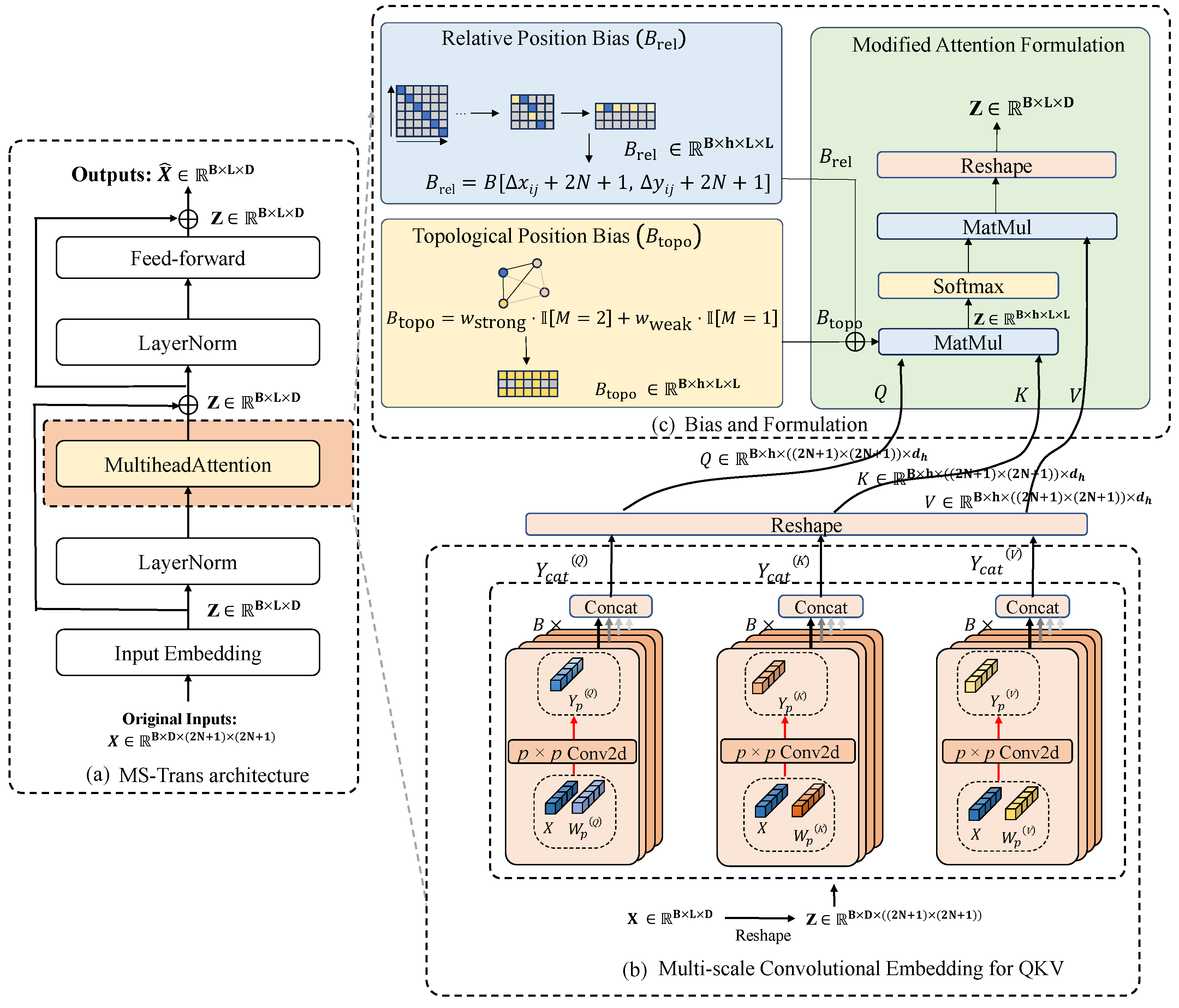
Standard Transformer architectures, while powerful for sequence modeling, inherently lack the 2D spatial awareness needed to capture relationships central to board games. We propose MS-Trans to address this limitation (as shown in Figure 4). Unlike a straightforward adaptation of Vision Transformers (ViT), MS-Trans encodes the geometric rule that “the four edges of a box are strongly correlated” as a learnable bias. By generating queries (Q), keys (K), and values (V) through multi-scale convolutions and incorporating topological bias directly into the attention mechanism, MS-Trans captures the structural patterns of the board.

Figure 4. (a) The overall architecture of MS-Trans. (b) Multi-scale convolution applied to Q, K, and V for feature extraction, followed by channel-wise concatenation. (c) During attention computation, relative position and topological biases are incorporated into the attention scores to enhance spatial awareness.

Figure 4. (a) The overall architecture of MS-Trans. (b) Multi-scale convolution applied to Q, K, and V for feature extraction, followed by channel-wise concatenation. (c) During attention computation, relative position and topological biases are incorporated into the attention scores to enhance spatial awareness.

4.2.1. Multi-Scale Convolutional Embedding for QKV

In standard Transformer architectures, the Q, K, and V matrices are derived directly from sequence features through linear transformations. For an input sequence $X\in {\mathbb{R}}^{L\times D}$, Q, K, and V are computed as follows:

$$Q=X{W}_Q,K=X{W}_K,V=X{W}_V,$$

(5)

where $W_Q,W_K,W_V\in {\mathbb{R}}^{D\times d_h}$.

Standard Transformers lack the 2D spatial awareness that board game modeling requires, and we found that linear encoders struggle with structures like chains or loops. We therefore replace the linear projections for Q, K, and V with 2D convolutions at multiple kernel sizes to extract both local and global features. These multi-scale features are concatenated and projected back to the original embedding dimension via a linear transformation.

$$\begin{array}{cc}\hfill Y_P^{\left(Q\right)}& =\mathrm{Conv}2\mathrm{d}\left(W_P^{\left(Q\right)}\right),\hfill \\ \hfill Y_{\mathrm{cat}}^{\left(Q\right)}& =\mathrm{Concat}\left(Y_P^{\left(Q\right)}\right),\hfill \\ \hfill Y_P^{\left(K\right)}& =\mathrm{Conv}2\mathrm{d}\left(W_P^{\left(K\right)}\right),\hfill \\ \hfill Y_{\mathrm{cat}}^{\left(K\right)}& =\mathrm{Concat}\left(Y_P^{\left(K\right)}\right),\hfill \\ \hfill Y_P^{\left(V\right)}& =\mathrm{Conv}2\mathrm{d}\left(W_P^{\left(V\right)}\right),\hfill \\ \hfill Y_{\mathrm{cat}}^{\left(V\right)}& =\mathrm{Concat}\left(Y_P^{\left(V\right)}\right).\hfill \end{array}$$

(6)

4.2.2. Relative Position and Topological Bias in Attention Mechanism

We adopt the 2D relative position bias used in Swin Transformer. This mechanism encodes the relative coordinate offsets between any two points by querying a learnable parameter table B. We integrate this as a relative position bias, denoted as $B_{\mathrm{rel}}$, which explicitly captures local neighborhood information.

$$B_{\mathrm{rel}}=B[\Delta x_{ij}+2N+1,\Delta y_{ij}+2N+1].$$

(7)

However, standard relative position bias fails to capture the unique geometric constraints of Dots-and-Boxes. To address this, we supplement the architecture with a specialized topological bias. We utilize a predefined adjacency mask, $M_{\mathrm{topo}}\in {\mathbb{R}}^{L\times L}$, to categorize connection strengths. Specifically, we define masks for strong connections ($M_{\mathrm{strong}}$ where $M_{\mathrm{topo}}=2$) and weak connections ($M_{\mathrm{weak}}$ where $M_{\mathrm{topo}}=1$). These logical priors are modulated by learnable scalar weights, $w_{\mathrm{strong}}$ and $w_{\mathrm{weak}}$, yielding:

$$B_{\mathrm{topo}}=w_{\mathrm{strong}}·\mathbb{I}[M_{\mathrm{topo}}=2]+w_{\mathrm{weak}}·\mathbb{I}[M_{\mathrm{topo}}=1].$$

(8)

By incorporating both relative position and topological biases into the attention scores, we obtain:

$$\mathrm{Attention}(Q,K,V)=\mathrm{Softmax}\left({\displaystyle \frac{Q{K}^T}{\sqrt{d}}}+B_{\mathrm{rel}}+B_{\mathrm{topo}}\right)V.$$

(9)

These learnable biases allow the model to decouple different features. Certain attention heads can specialize in relative positional information, while others focus on the structural information of the board itself.

4.2.3. ResidualBlock–TransformerBlock Hybrid Architecture

Dots-and-Boxes gameplay relies on both short-term tactics and long-term structural planning. ResidualBlocks excel at extracting local patterns but struggle with global dependencies, while TransformerBlocks capture long-range information effectively but may lack precision in local feature refinement.

To balance these requirements, we evaluate four distinct architectures, Baseline, TT, RT, and TR, composed of different arrangements of residual and Transformer blocks. Additionally, we introduce a dimension conversion module to bridge the dimensional mismatch between these two block types.

Definition 1.

We define the evaluated architectures as follows:

• Baseline:
  Serves as the performance standard, consisting of a pure stack of 6 ResidualBlocks.
• TT: To isolate the effect of removing convolutional locality, this model replaces the 6 ResidualBlocks of the baseline entirely with 6 TransformerBlocks.
• RT: This hybrid architecture sequences two ResidualBlocks followed by one TransformerBlock, repeating this unit. This design prioritizes the refinement of local features before integrating them into a global context.
• TR: This hybrid architecture inverts the sequence of the RT architecture, placing a TransformerBlock before two ResidualBlocks. This configuration attempts to capture global context early in the network, which then informs the local feature processing.

4.3. Auxiliary Training Tasks

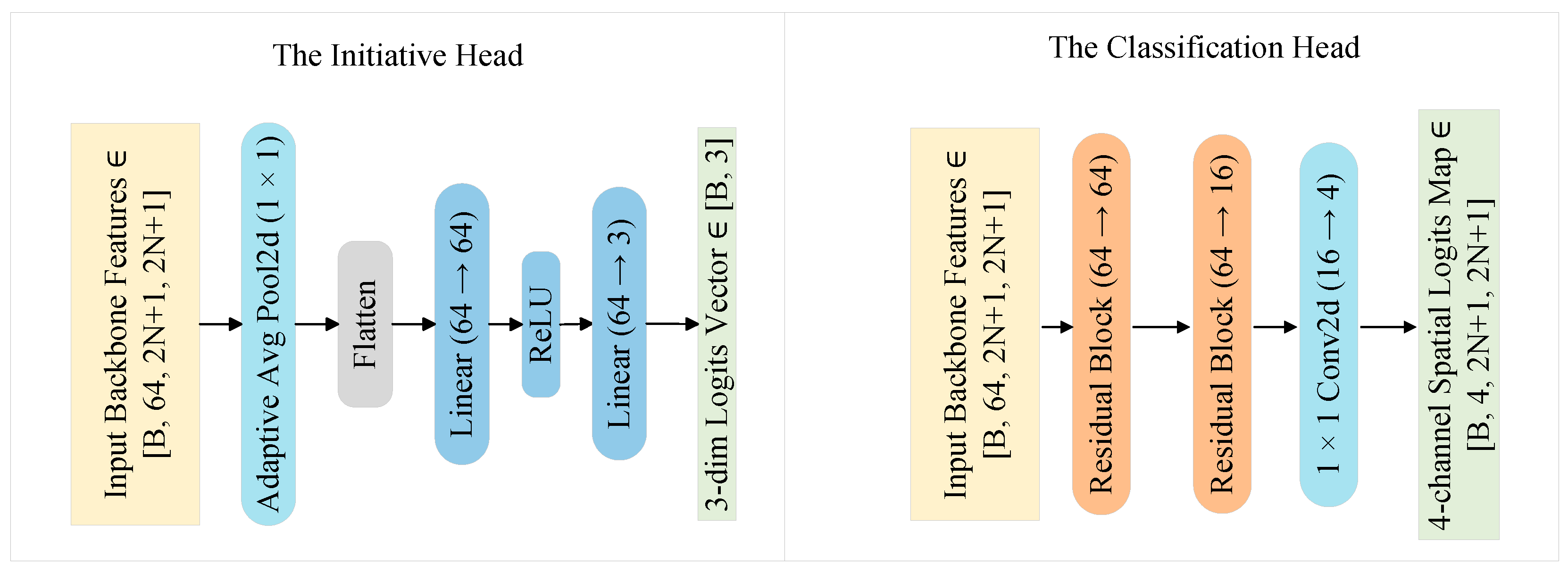
In board games, a model must not only learn policies and value functions but also understand the spatial structure of the board and the rules governing legal moves. Training a policy network directly often suffers from data sparsity, slow convergence, and difficulty in internalizing game rules. Auxiliary training tasks can provide additional supervisory signals during early training, such as initiative prediction or move classification. This enables the model to rapidly acquire basic game mechanics, thereby improving the efficiency of subsequent policy learning. The neural network architecture for the auxiliary training tasks is shown in Figure 5.

4.3.1. Initiative Prediction

In Dots-and-Boxes, the decision to retain or relinquish the initiative can decisively affect the result of a game. Strategic questions arise, such as “Should I capture all available boxes, thereby relinquishing the initiative for immediate points?” or “Should I sacrifice certain boxes, thereby retaining the initiative to constrain the opponent?” Therefore, predicting “whether the initiative should be retained or relinquished” is a critically important auxiliary task. The process is illustrated in Figure 2.

Definition 2.

We categorize single-step decision behaviors into three classes and formalize them as the vector set $v\in \{v_{\mathrm{k}},v_{\mathrm{s}},v_{\mathrm{n}}\}$:

• Capture:
  If an immediate box completion (and thus immediate scoring while relinquishing the initiative) is available, we denote this situation as $v_{\mathrm{k}}=(1,0,0)$.
• Sacrifice: If an immediate box completion is available but the player deliberately refrains from taking it, we denote this situation as $v_{\mathrm{s}}=(0,1,0)$. This might occur, for example, to lure the opponent or to better control the board state.
• Neutral: If no immediate box completion is available and the player can only draw an ordinary edge without scoring, we denote this situation as $v_{\mathrm{n}}=(0,0,1)$.

4.3.2. Classification Prediction

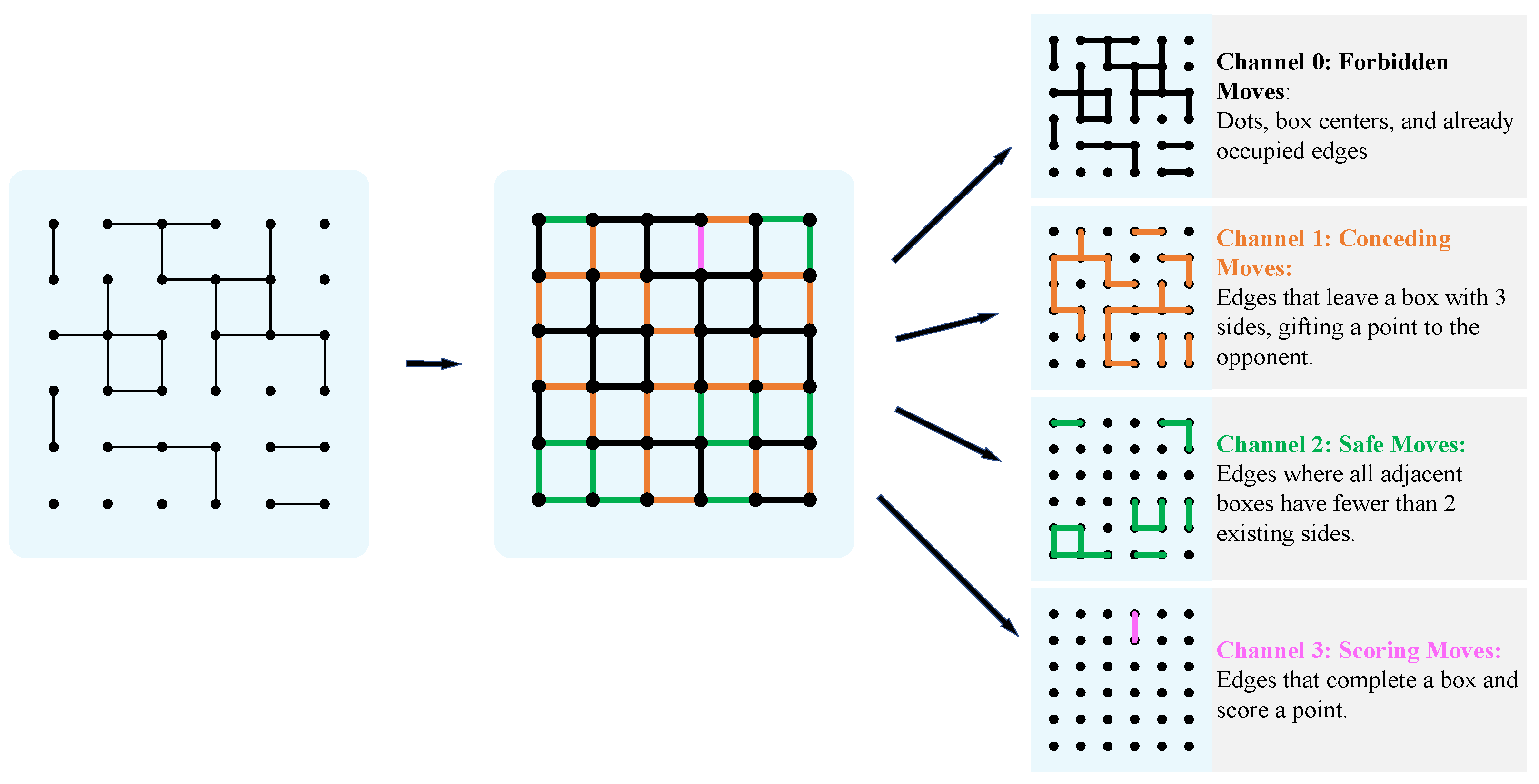
We designed a classification task that categorizes different types of moves, encouraging the neural network to quickly learn the rules of the game. We formulate this as a four-way classification problem that encourages the network to distinguish among forbidden, conceding, safe, and scoring moves. The process is shown in Figure 6.

Definition 3.

We partition the action space into four mutually exclusive categories. For an action e at a given state, the category is determined as follows:

• Forbidden Moves: An action is considered invalid if it selects a dot or a box center or an edge $\forall e\in E_{\mathrm{occupied}}$, where $E_{\mathrm{occupied}}$ represents the set of already occupied edges.
• Conceding Moves: An action that creates at least one adjacent box with three occupied edges, thereby allowing the opponent to score on the next turn, i.e.,

  $$\forall e\notin E_{\mathrm{occupied}}\mathrm{AND}\exists b\in N\left(e\right),k\left(b\right)=2,$$

  where $N\left(e\right)$ is the set of boxes adjacent to edge e, and $k\left(b\right)$ is the number of current occupied edges for the box b.
• Safe Moves: An action after which none of the adjacent boxes is placed into an opponent-scoring state, i.e.,

  $$\forall e\notin E_{\mathrm{occupied}}\mathrm{AND}\forall b\in N\left(e\right),k\left(b\right)<2.$$
• Scoring Moves: An action that completes a box and therefore yields an immediate score, i.e.,

  $$\forall e\notin E_{\mathrm{occupied}}\mathrm{AND}\exists b\in N\left(e\right),k\left(b\right)=3.$$

4.4. Neural Network Architecture

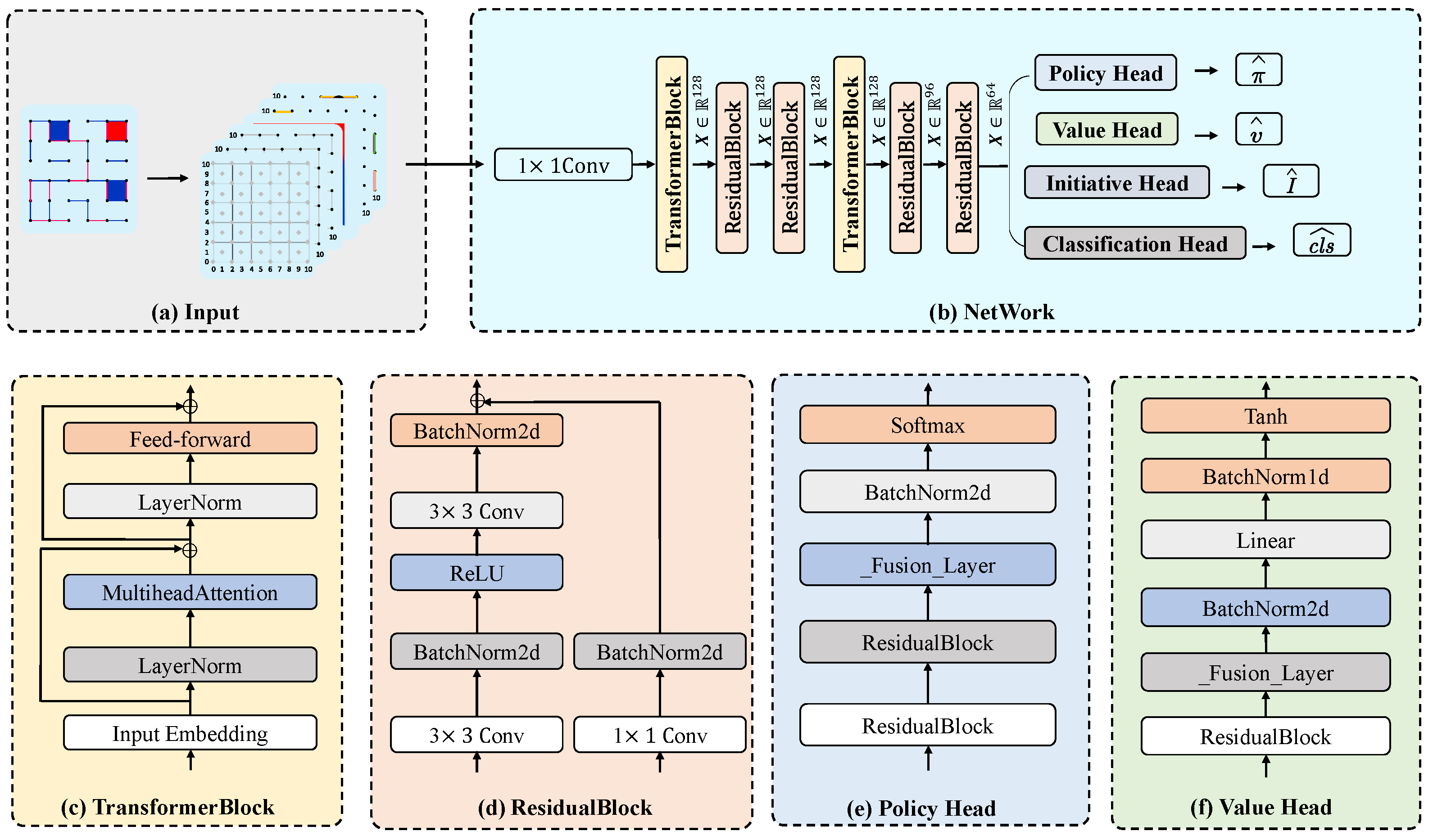
The neural network architecture employed in this work is primarily composed of a combination of Transformer modules and residual CNNs. This design balances global strategic modeling with local feature extraction, as shown in Figure 7. The _Fusion_Layer is a custom fusion layer that performs a weighted fusion of multi-channel features via a learnable weight matrix. It converts the input $C\times (2N+1)\times (2N+1)$ feature maps into a $1\times (2N+1)\times (2N+1)$ output. This effectively integrates spatial information from all channels, providing a refined feature representation for policy and value prediction.

5. Experiments

5.1. Experimental Setup

5.1.1. DATASET

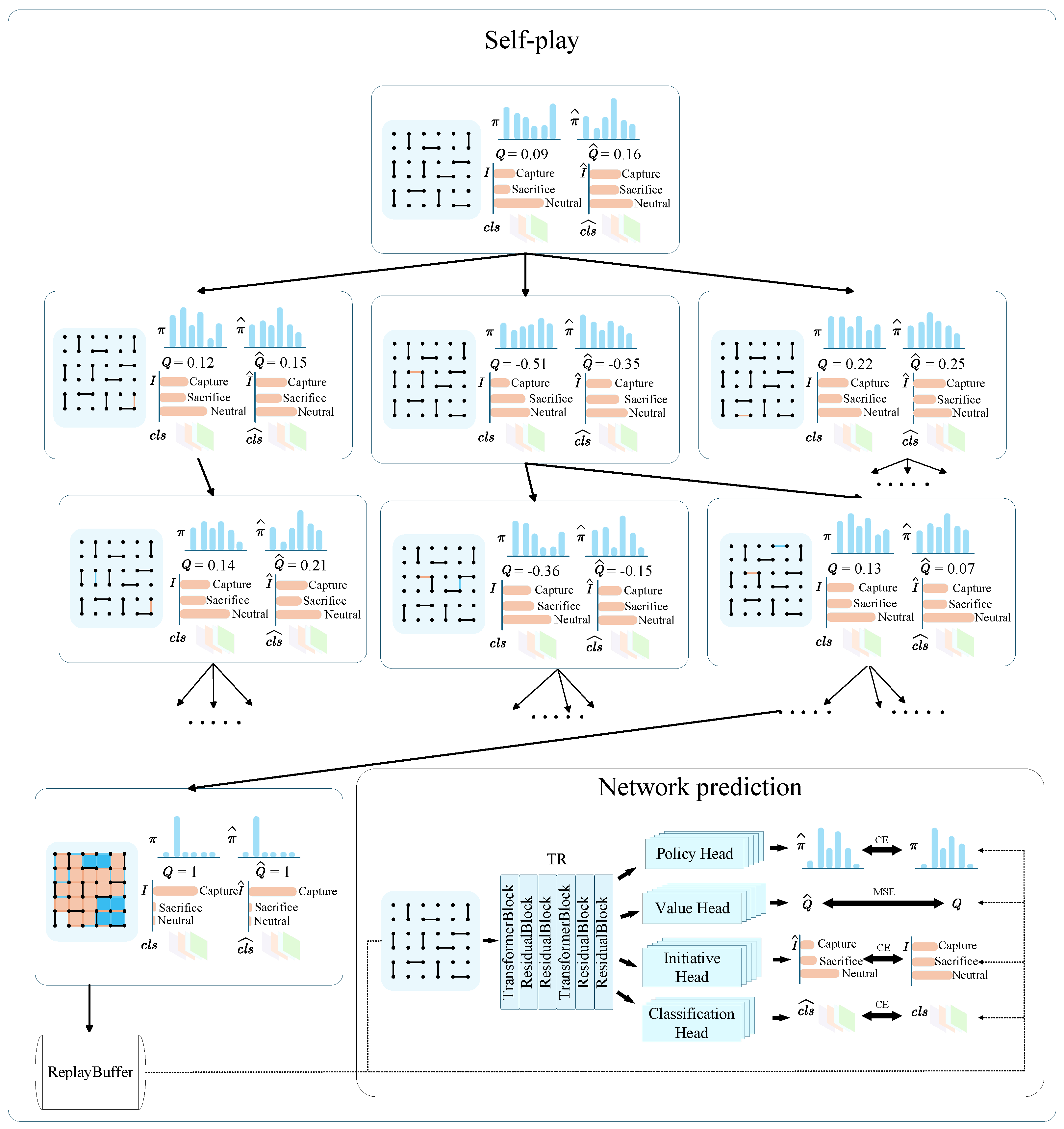
As shown in Figure 8, during the training phase, self-play is employed to generate training data. At each decision step, MCTS is used to compute the optimal move probability distribution $\pi$ for the current board state, along with the final game outcome Q, the initiative I, and the classification label $cls$. The classification vector $cls$ is represented in a simplified form in Figure 8, with a visual explanation shown in Figure 5.

The replay buffer stores data generated from self-play, including $(\mathrm{board},\pi ,Q,I,cls)$, and only keeps samples from recent iterations. During training, data are randomly sampled from the buffer, which helps reduce temporal correlation between samples. In addition, a decay weight ${\gamma }_{\mathrm{decay}}$ is introduced according to the iteration when the data were generated, so that more recent samples receive higher importance. This encourages the model to focus on the latest policy distribution. As a result, the overall data efficiency is improved, and the training process becomes more stable.

5.1.2. Baseline

The baseline used in our experiments is not a direct reproduction of the AlphaZero [3] Go version. Instead, it is an AlphaZero architecture adapted and optimized for the Dots-and-Boxes task. Given that the board size in our setting is 5 × 5, which is much smaller than the 19 × 19 Go board, directly adopting a 20-layer residual network would lead to an unnecessarily large number of parameters. Therefore, we employ a 6-layer residual network as the backbone of the baseline, whose parameter size (1.42 M) is comparable to that of Dotsformer (1.94 M). The detailed configurations in architecture are summarized in

Table 3. Comparison of Baseline and Dotsformer configurations.

Feature	Baseline (AlphaZero)	Dotsformer (Proposed)
Backbone	6 residual blocks	MS-Trans (6-layer Hybrid TR-structure)
Parameters	1.42 M	1.94 M
Policy Head	2× Res + Fusion + BN + Softmax	Same
Value Head	Res+ Fusion + BN + Linear + BN + Tanh	Same
Search Budget	800 simulations/move	Same
Training Budget	4500 self-play games	Same

. To ensure a fair comparison and eliminate the influence of non-essential factors, the baseline and Dotsformer share the same policy/value head design, MCTS search budget (800 simulations per move), and the same amount of self-play training data (4500 games). Other hyperparameters, such as Cpuct (1.0), learning rate (0.001), and batch size (1024), are also kept identical. The full configuration details are provided in Appendix

Table A1. Hyperparameter settings used during training.

Category	Parameter	Value	Description
MCTS search	$N_{\mathrm{sim}}$	800	Number of MCTS simulations per move
	$\tau$	0.4	Temperature parameter of the policy distribution
	$c_{\mathrm{puct}}$	1.0	Exploration constant used in PUCT
Rollback strategy	$T_{\mathrm{start}}$	32	Step threshold at which incremental training begins
	${\Delta }_{\mathrm{step}}$	1	Step interval for sample generation
	${\Delta }_{\mathrm{iter}}$	10	Iteration interval for sample generation
Experience replay	$N_{\mathrm{thresh}}$	100	Threshold on node visit counts
	$Q_{\mathrm{thresh}}$	0.8	Threshold on the average node value
	$D_{\min }$	$5\times {10}^6$	Minimum number of states stored in the replay buffer
	$G_{\min }$	5	Minimum number of games per iteration
	${\gamma }_{\mathrm{decay}}$	0.9	An experience decay factor
Optimizer	$lr$	${10}^{-3}$	Initial learning rate
	$\lambda$	${10}^{-5}$	L2 regularization coefficient
	$I_{\mathrm{decay}}$	80	Iteration threshold for halving the learning rate
Training	Epochs	5	Number of training epochs per iteration
	$\mathrm{Batch}\mathrm{size}$	1024	Training batch size
Loss weights	${\lambda }_{\pi }$	1.0	Weight of the policy loss
	${\lambda }_v$	$\sqrt{11}$	Weight of the value loss
	${\lambda }_{\mathrm{reg}}$	${10}^{-4}$	Weight of the regularization term
	${\lambda }_I$	$\sqrt{11}$	Weight of the initiative loss
	${\lambda }_{cls}$	10.0	Weight of the classification loss

.

5.2. EdgeQuad and ChainLoop: Evaluating Feature Representation in Self-Play Games

5.2.1. Impact of Feature Representation on Model Efficiency

Table 4. Effects of Different Board Representation Configurations on the Efficiency of Baseline, EdgeQuad, and ChainLoop Models.

Model	FLOPs (G)	Params (M)	Latency (ms)
Baseline	0.172	1.42	1.67 [0.14, 0.23]
EdgeQuad4	0.035	1.42	2.89 [0.26, 0.54]
EdgeQuad9	0.035	1.42	2.84 [0.18, 0.34]
EdgeQuad44	0.036	1.47	2.86 [0.31, 0.43]
ChainLoop64	0.181	1.50	1.67 [0.16, 0.22]
ChainLoop6	0.172	1.42	1.66 [0.14, 0.22]

compares the computational efficiency of the baseline, EdgeQuad, and ChainLoop architectures across different board representations. We evaluated FLOPs (GFLOPs), Parameters (M), and Average Latency (ms). Average Latency refers to the average time required for a single forward pass of the neural network. In practice, EdgeQuad incurs higher average latency than the baseline, indicating that the introduced feature organization does not improve inference efficiency in an end-to-end setting. In contrast, the metrics of ChainLoop are very close to those of the baseline, indicating that ChainLoop introduces little additional computational overhead. The reported latency is the mean across four random seeds, with the within-seed standard deviation range defined as the minimum and maximum standard deviations among the four seeds. The seeds used are 42, 100, 200, and 300.

5.2.2. ELO Score: Feature Representation Evaluation

Each model was trained over approximately 4500 self-play games. Each iteration consisted of 30 games, yielding approximately 150 iterations and a total of roughly 270,000 game states. During training, all models used 800 MCTS simulations per move; during evaluation, this was reduced to 400. During training, we recorded the number of iterations required to roll back the MCTS starting step while meeting the predefined performance criteria. The results are summarized in

Table 5. Training Iterations Required for Stepwise Rollback of the MCTS Starting Step in Feature Representation Model.

Model	Step
	32nd	31st	30th	29th	28th	27th	26th	25th	24th
Baseline	49	59	69	79	90	100	stop	stop	stop
EdgeQuad4	12	stop	stop	stop	stop	stop	stop	stop	stop
EdgeQuad9	77	106	stop	stop	stop	stop	stop	stop	stop
EdgeQuad44	74	93	126	stop	stop	stop	stop	stop	stop
ChainLoop64	23	33	46	56	66	76	106	stop	stop
ChainLoop6	21	32	42	53	64	74	109	119	stop

Note: “Stop” indicates that the rollback process terminates at this step and cannot proceed further.

. During evaluation, models competed against each other in Dots-and-Boxes. Each game had 60 moves in total, and a pruning strategy was used to guide the first 15 moves.

The baseline, EdgeQuad4, EdgeQuad9, EdgeQuad44, ChainLoop64, and ChainLoop6 models all began with MCTS initialized at step $S_{\mathrm{start}}$. When the rollback condition was satisfied and the interval since the previous rollback exceeded $\Delta t$, the starting step was rolled back by $\Delta S$. This process was repeated iteratively. For each step, the reported iteration count indicates the number of training iterations required to roll back the MCTS starting step from this step to the next earlier step, rather than to reach this step.

The experimental results show that, despite their lower FLOPs, the EdgeQuad models exhibit the weakest rollback capability overall. As more board representation information is introduced, its rollback capability improves gradually from 4 to 9 and then to 44 channels. Even so, the starting point can only be rolled back to step 29 and remains fixed at this step thereafter. In contrast, the ChainLoop models demonstrate more stable and stronger rollback behavior. The starting point could be rolled back to as far as step 24, with performance consistently surpassing that of the baseline. ChainLoop6 demonstrates the strongest performance, achieving higher rollback depth. For the same rollback target step, it typically requires fewer training iterations.

We evaluated six board representation schemes for Dots-and-Boxes under controlled experimental conditions. Each model played 500 games against every other model, for a total of 7500 games.

Table 6. ELO Score in Feature Representation Model.

Model	ELO	Win Rate	95% Confidence Interval
Baseline	1746	73.28%	[71.55%, 75.01%]
ChainLoop6	1855	83.00%	[81.53%, 84.47%]
ChainLoop64	1784	75.96%	[74.29%, 77.63%]
EdgeQuad44	1259	28.56%	[26.79%, 30.33%]
EdgeQuad9	1207	23.44%	[21.78%, 25.10%]
EdgeQuad4	1148	15.76%	[14.33%, 17.19%]

and

Table 7. Detailed Win Rate in Feature Representation Model.

Model	Baseline	ChainLoop6	ChainLoop64	EdgeQuad44	EdgeQuad9	EdgeQuad4
Baseline	NA	38.80%	46.40%	89.60%	95.60%	96.00%
ChainLoop6	61.20%	NA	63.40%	94.40%	97.20%	98.80%
ChainLoop64	53.60%	36.60%	NA	95.20%	96.20%	98.20%
EdgeQuad44	10.40%	5.60%	4.80%	NA	57.40%	64.60%
EdgeQuad9	4.40%	2.80%	3.80%	42.60%	NA	63.60%
EdgeQuad4	4.00%	1.20%	1.80%	35.40%	36.40%	NA

Note: “NA” indicates that the entry is not applicable, as a method is not compared with itself.

present the final scores. ChainLoop6 achieves the highest performance, with an average win rate of 83.00%. Against the baseline, it reaches a win rate of 61.20%. Compared with the EdgeQuad variants, the ChainLoop models achieve higher ELO scores. This suggests that ChainLoop representations offer advantages in boundary control, anticipating chain reactions, and evaluating the global game state.

5.3. Effects of Individual Components in the MS-Trans Architecture

5.3.1. A Comparative Analysis of Hybrid Residual-Transformer Architectures

Table 8. Training Iterations Required for Stepwise Rollback of the MCTS Starting Step in ResidualBlock–TransformerBlock Hybrid Architecture Model.

Model	Step
	32nd	31st	30th	29th	28th	27th	26th	25th	24th
Baseline	49	59	69	79	90	100	stop	stop	stop
RT	16	26	37	47	57	89	106	129	stop
TR	17	27	37	50	63	84	97	107	stop
TT	41	55	65	82	stop	stop	stop	stop	stop

shows how many training iterations each model needed to roll back the MCTS starting step using the rollback strategy described above, while meeting the target performance criteria.

Rollback in the baseline model is limited in depth. Its starting point can be rolled back only to step 26, requiring 100 iterations, and the rollback process stops at this step. In comparison, the TR model achieves the deepest rollback, stably reaching step 24 after 107 iterations. The RT model also reaches step 24, but requires 129 iterations. Moreover, the number of iterations needed at each stage is consistently higher than for TR, reflecting lower efficiency. The TT model is the weakest, rolling back only to step 28. In summary, the TR model performs best, achieving the fastest rollback. In comparison, the baseline and TT models perform poorly with limited rollback capability (baseline, RT, TR, and TT are defined in Definition 1).

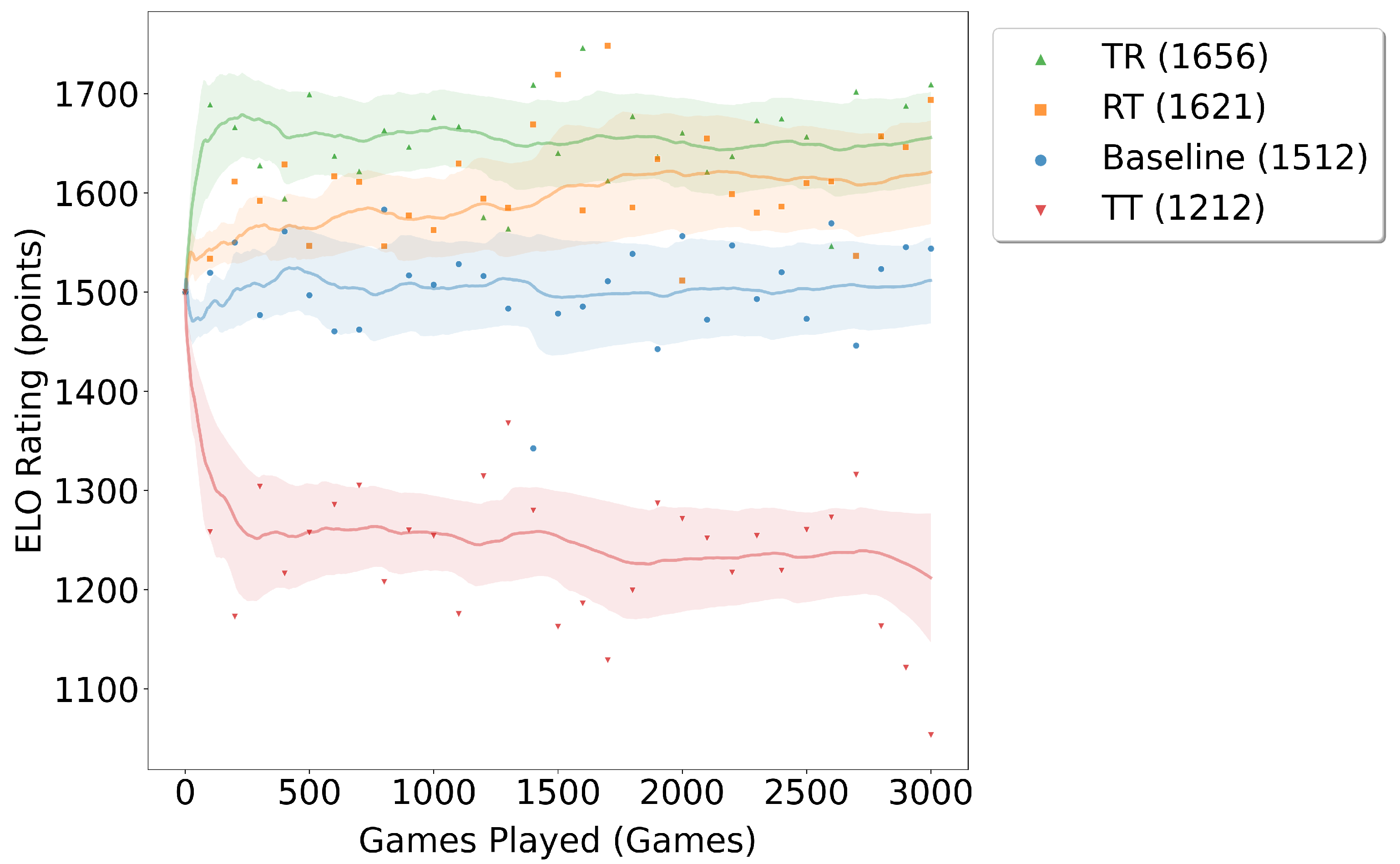
Each model played 500 games against every other model, for a total of 3000 games. The ELO ratings for each model are shown in Figure 9.

The experimental results show that the TR model achieves the highest performance, with an ELO of 1656. Compared with the TT and the baseline model, the TR and RT models combine residual CNNs and Transformers to extract local and global features.

5.3.2. Evaluation of Multi-Scale QKV Convolution with Topological Bias

This training uses the same rollback strategy described above, applied to architectures that combine the TR model with the ChainLoop6 feature representation.

Table 9. Training Iterations Required for Stepwise Rollback of the MCTS Starting Step in MultiScale-Topo Model.

Model	Step
	32nd	31st	30th	29th	28th	27th	26th	25th	24th	23rd	22nd
Linear-NoTopo	10	20	30	44	54	81	97	107	129	stop	stop
MultiScale2-Topo	10	20	30	41	51	61	74	106	116	stop	stop
MultiScale4-Topo	11	21	31	41	51	62	73	95	121	139	stop

reports the number of training iterations required for each model to roll back the MCTS starting step in these architectures.

The results show that the MultiScale4-Topo model exhibits the strongest rollback capability, stably reaching step 22. The MultiScale2-Topo model ranks second in rollback performance, performing better than Linear-NoTopo but below MultiScale4-Topo. Linear-NoTopo is built on the TR architecture combined with the ChainLoop6 feature representation. It can roll back to step 23. In comparison, the ChainLoop6 model alone can only reach step 24, and the TR model alone is also limited to step 24. These results indicate that integrating the TR model with the ChainLoop6 representation improves rollback capability.

Working together, these two components enable more accurate evaluation of earlier game states and support deeper rollback during training.

The results in

Table 10. Performance Evaluation of MultiScale4-Topo, MultiScale2-Topo, and Linear-NoTopo: ELO Rating and Win Rate.

Model	ELO	Win Rate	95% Confidence Interval
MultiScale4-Topo	1618	71.67%	68.0–75.3%
MultiScale2-Topo	1562	63.33%	59.3–67.3%
Linear-NoTopo	1420	45%	40.8–49.2%

indicate that performance improves as the convolutional scale increases. Among the models, MultiScale4-Topo achieves a higher win rate and ELO rating compared to MultiScale2-Topo and Linear-NoTopo. This demonstrates the effectiveness of the multi-scale QKV convolution structure combined with the topological bias. However, due to its larger number of parameters, MultiScale4-Topo trains more slowly; therefore, the smaller MultiScale2-Topo is used in the ablation studies.

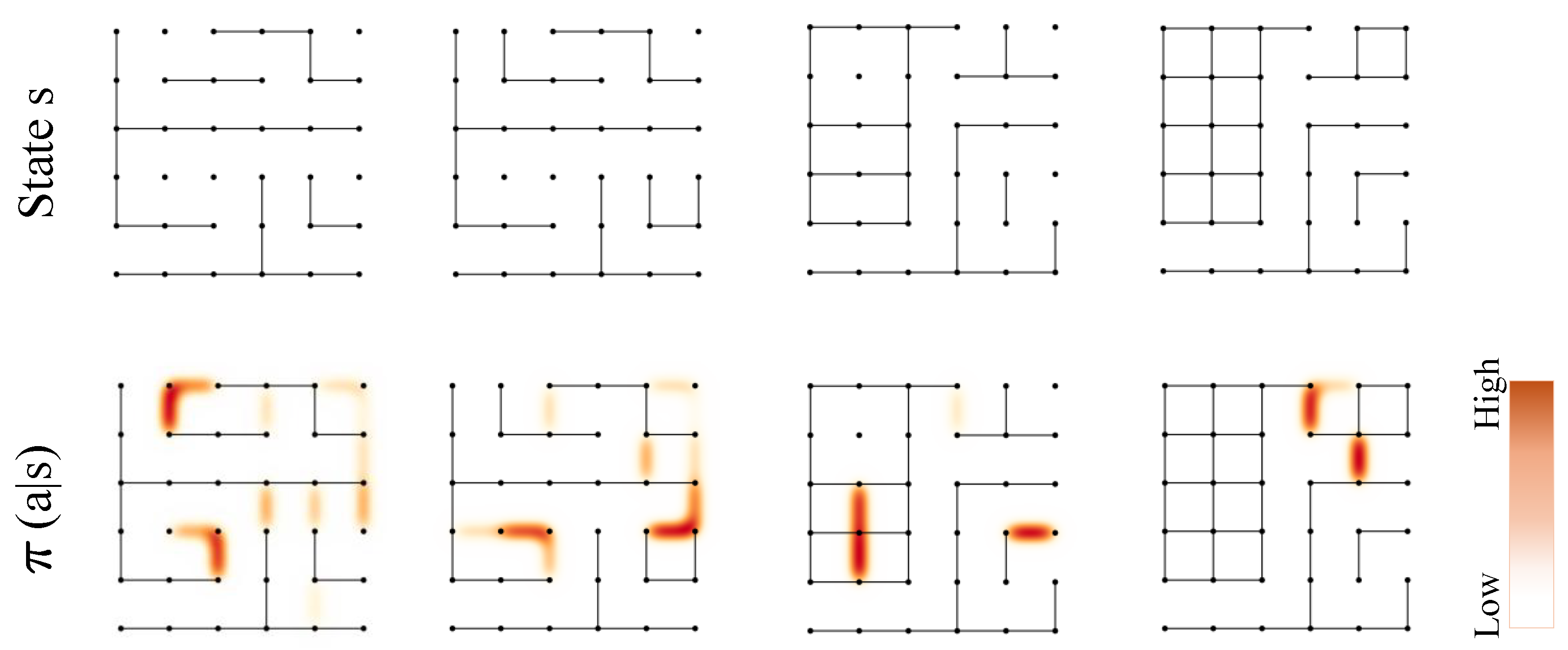
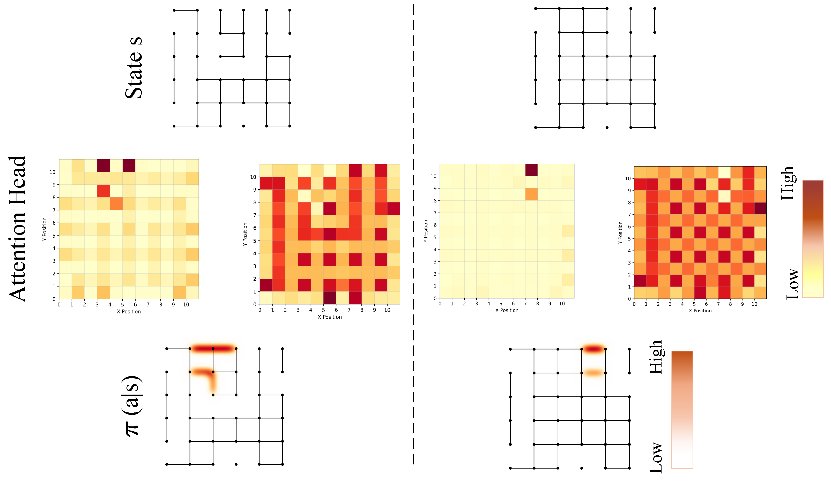
To investigate the decision-making logic of the model, we visualized the attention maps of the Transformer model on representative Dots-and-Boxes game states, as shown in Figure 10. In the first game state, the model distributes its attention across many candidate edges. After two subsequent moves, one box has three edges occupied, and the model focuses strongly on the remaining fourth edge, indicating that it can identify immediate scoring opportunities.

In the next two states, the attention maps show that the model looks not only at edges that can score right away but also at moves that temporarily give up a box to keep the initiative. This suggests it plans ahead, weighing longer-term benefits beyond immediate points. A detailed analysis is given in Appendix D.

5.4. Additional Evaluation Metrics and Analysis

5.4.1. Analysis of Different Loss Functions Curve

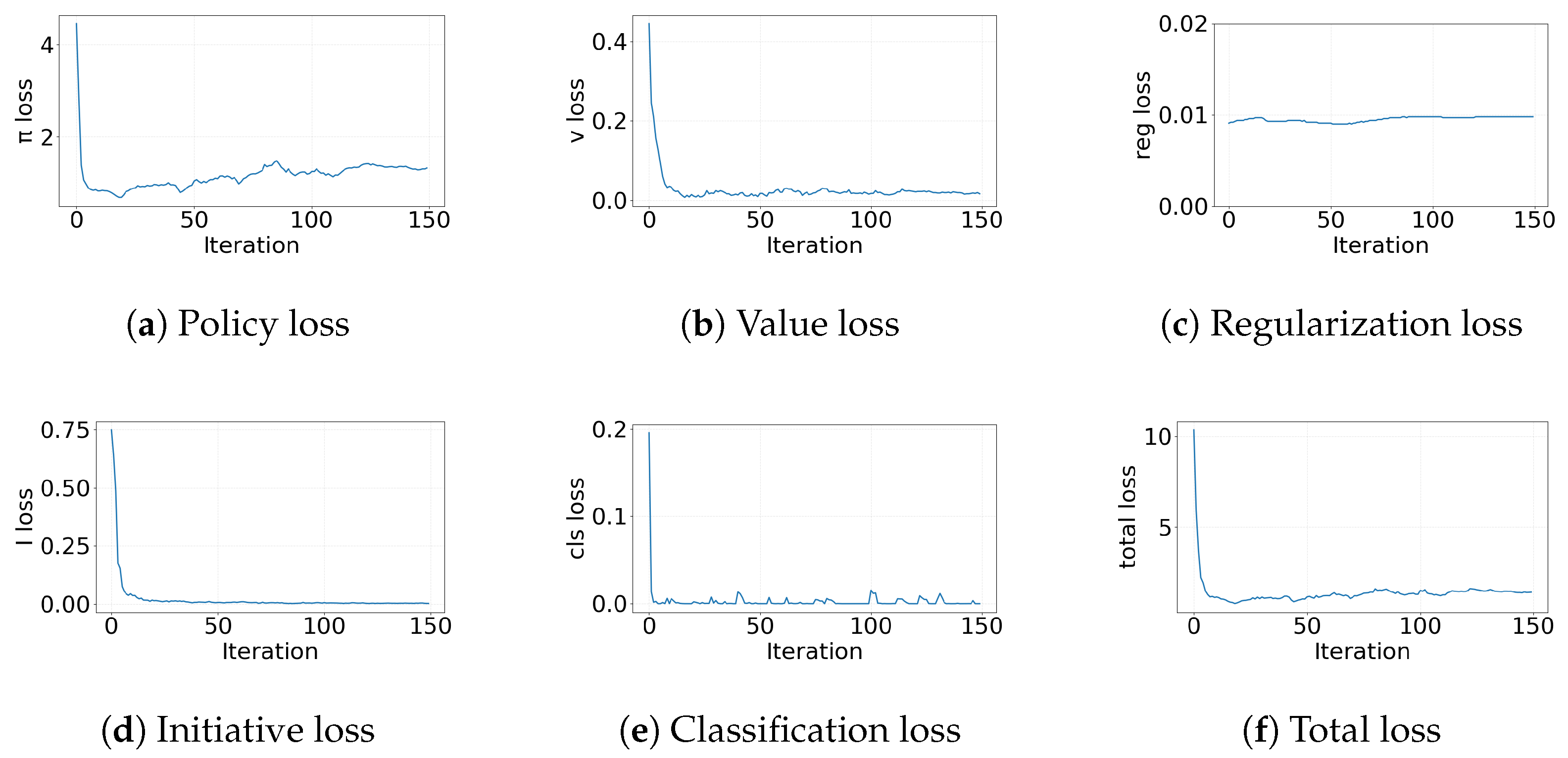
As shown in Figure 11, MCTS initially starts from move 32, near the endgame, where policy learning is relatively straightforward. This results in low initial policy loss. As the search starting point moves to earlier game stages, policy prediction becomes more difficult, causing a slight increase in policy loss. Meanwhile, the value loss and initiative loss drop noticeably, and the regularization loss stays roughly the same.

At the same time, the classification loss converges from 0.2 to near 0. The initial value and scale of this loss are relatively small because the contribution of channel 1 is excluded during computation, allowing the model to focus on classification errors in regions relevant to decision-making. This design ensures rapid convergence while effectively reducing interference from background noise.

Notably, loss functions reduce rapidly during the early stage since our training is from the endgame, which is easy to learn.

5.4.2. Comparison of Dotsformer and AlphaZero in Terms of $N_{\mathrm{root}}^{\mathrm{corr}}$/$N_{\mathrm{root}}^{\mathrm{total}}$ and $N_{\mathrm{step}}^{\mathrm{corr}}$/$N_{\mathrm{step}}^{\mathrm{total}}$

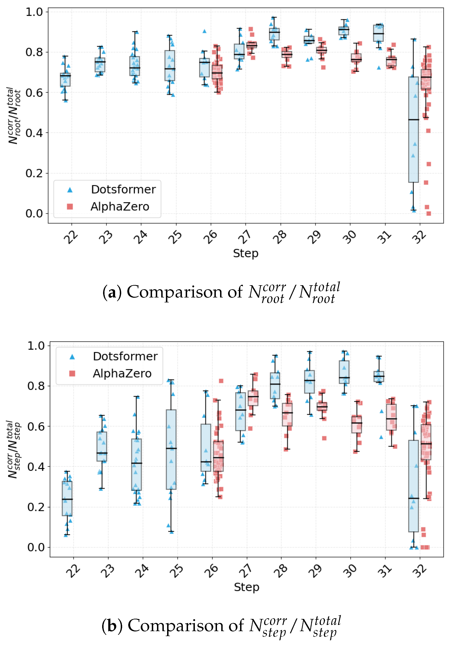
For moves closer to the end of the game, the network can more clearly distinguish winning from losing states, so the MCTS metrics $N_{\mathrm{root}}^{\mathrm{corr}}/N_{\mathrm{root}}^{\mathrm{total}}$ and $N_{\mathrm{step}}^{\mathrm{corr}}/N_{\mathrm{step}}^{\mathrm{total}}$ gradually rise during training and reach the thresholds ${\tau }_{\mathrm{root}}$ and ${\tau }_{\mathrm{step}}$. For moves farther from the end, distinguishing outcomes is more difficult. These metrics seldom reach the thresholds even as training continues.

Figure 12 shows that Dotsformer achieves higher $N_{\mathrm{root}}^{\mathrm{corr}}/N_{\mathrm{root}}^{\mathrm{total}}$ and $N_{\mathrm{step}}^{\mathrm{corr}}/N_{\mathrm{step}}^{\mathrm{total}}$ than AlphaZero on the majority of steps, while requiring fewer iterations to reach comparable performance. It also reaches the ${\tau }_{\mathrm{root}}$ and ${\tau }_{\mathrm{step}}$ thresholds more easily, allowing more frequent rollback. As iterations increase, Dotsformer continues to roll back, while AlphaZero gradually fails to meet the rollback condition and stops.

This indicates that Dotsformer evaluates midgame positions more accurately, enabling it to better discriminate strong moves and improve search efficiency. As a result, the model guides the expansion of the search tree more effectively during the midgame, avoiding unnecessary exploration.

5.5. Ablation Studies

Using the same rollback strategy as described earlier,

Table 11. Training Iterations Required for Stepwise Rollback of the MCTS Starting Step in Ablation Studies.

Model	Step
	32nd	31st	30th	29th	28th	27th	26th	25th	24th	23rd	22nd	21st
Baseline	49	59	69	79	90	100	stop	stop	stop	stop	stop	stop
No-MS-Trans	24	34	44	54	64	74	89	125	stop	stop	stop	stop
No-ChainLoop6	14	25	35	45	55	87	98	117	141	stop	stop	stop
No-Auxiliary	10	20	30	40	50	68	80	104	114	stop	stop	stop
Full	10	20	30	40	50	60	70	85	109	126	152	stop

reports the number of iterations required for each model to advance the MCTS starting step while maintaining the target performance.

The baseline shows the weakest rollback ability. Starting from step 32, it could roll back only to step 26 after 100 iterations and stopped thereafter. Models without specific components show moderate performance: No-MS-Trans, No-ChainLoop6, and No-Auxiliary roll back to steps 24, 23, and 23, respectively. The full model demonstrates the strongest rollback capability, achieving the deepest rollback to step 21 among all models. It also requires fewer iterations to reach each rollback step compared with the other models, indicating the highest training efficiency and the strongest ability to optimize strategies.

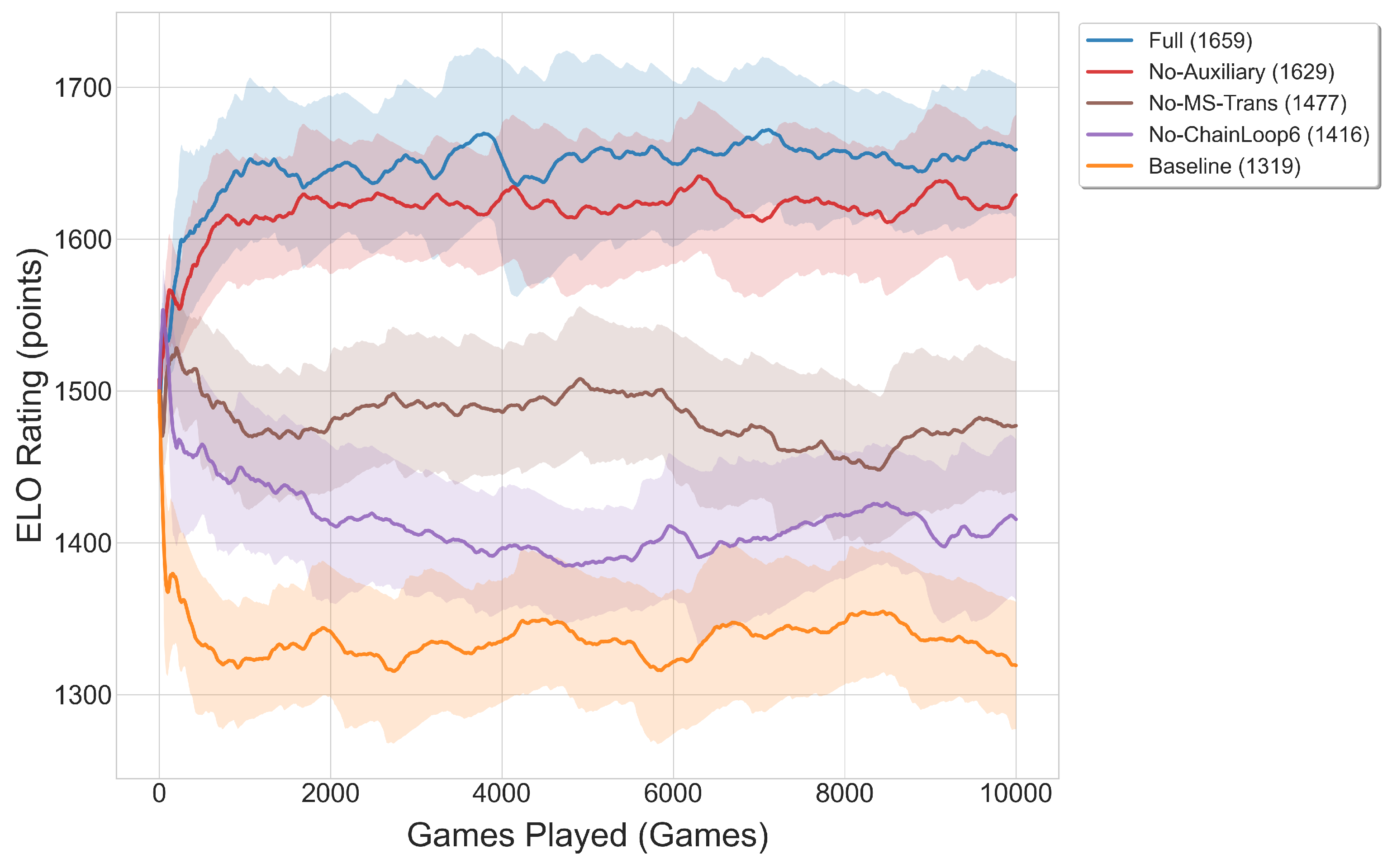
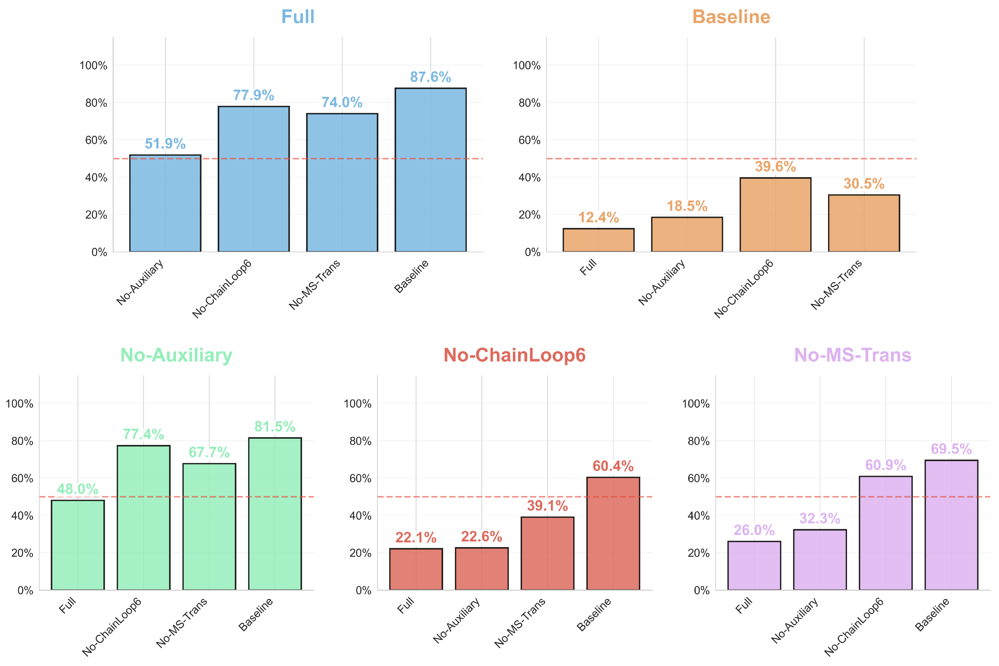
To evaluate the effectiveness of individual components, we conducted extensive ablation studies. Each model played 1000 games against every other model, resulting in a total of 10,000 matches. The ELO scores and the average win rates of all models are reported in

Table 12. Performance Evaluation of Ablation Studies: ELO Rating and Win Rate.

Model	ELO	Win Rate	95% Confidence Interval
Full	1659	72.85%	[71.47%, 74.23%]
No-Auxiliary	1629	68.65%	[67.21%, 70.09%]
No-MS-Trans	1477	47.17%	[45.63%, 48.71%]
No-ChainLoop6	1416	36.05%	[34.56%, 37.54%]
Baseline	1319	25.25%	[23.90%, 26.60%]

. The ELO score distributions are illustrated in Figure 13, while the detailed pairwise win rate results are shown in Figure 14.

The experimental results demonstrate that the Full model achieves the best overall performance, with an ELO score of 1659 and an average win rate of 72.85%. In particular, its win rate against the baseline reaches 87.6%. After removing certain optimization components, model performance declines to varying extents. Figure 14 presents a comparison of win rates for different models against the baseline. Specifically, the win rates of No-ChainLoop6, No-MS-Trans, No-Auxiliary, and Full against the baseline are 60.4%, 69.5%, 81.5%, and 87.6%, respectively. It indicates that removing any single module leads to a consistent degradation in performance, indicating that each component contributes positively to the overall model effectiveness. Among all variants, the Full model achieves the highest win rate and demonstrates the best performance.

We conducted four independent runs, each with 10 repetitions, using the same random seeds as in Table 4. According to

Table 13. Computational cost analysis of different model configurations.

Model	FLOPs (G)	Params (M)	Latency (ms)
Full	0.235	1.94	3.97 [0.34, 0.50]
No-Auxiliary	0.224	1.85	3.73 [0.26, 0.39]
No-MS-Trans	0.183	1.52	2.03 [0.09, 0.14]
No-ChainLoop6	0.235	1.94	3.98 [0.25, 0.52]
Baseline	0.172	1.42	1.73 [0.14, 0.23]

, compared with the baseline, the Full architecture introduces approximately 36% more parameters and computational cost. However, the average inference latency increases from 1.73 ms to 3.97 ms. Notably, after removing the ChainLoop6 module, the model’s FLOPs and latency remain nearly unchanged compared with the Full model, indicating that this module did not introduce an additional computational burden. This observation is consistent with the results reported in Table 4.

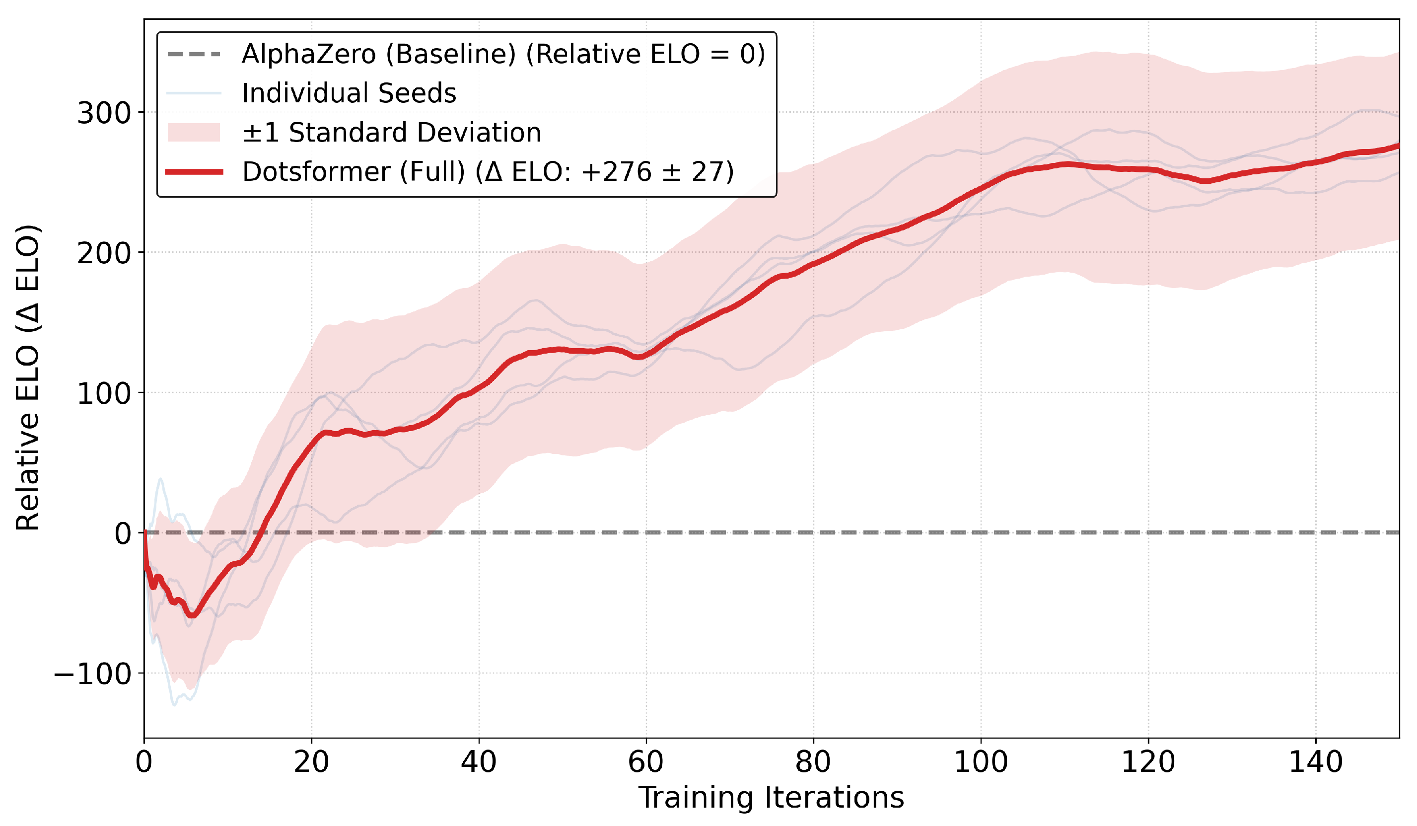
To validate the stability of our model’s performance and reduce the influence of randomness, we conducted independent evaluation experiments under four distinct random seeds (42, 100, 200, and 300). Each setting included 1000 games between Dotsformer and AlphaZero. Figure 15 shows the relative ELO progression of Dotsformer against the baseline over training iterations.

In the early stage, the relative ELO temporarily decreases. This is because both models are untrained at the beginning, making the game outcomes largely random. As training proceeds, the relative ELO steadily increases. The curves from different random seeds are closely aligned, indicating good training stability. To further validate the results, we conducted a statistical significance test on the final relative ELO scores across the four seeds. An independent t-test shows that Dotsformer achieves a statistical improvement over the baseline (p < 0.001).

5.6. Discussion

ChainLoop and Ms-Trans are the core designs of our method. ChainLoop explicitly encodes chain and loop structures, while Ms-Trans incorporates topological bias into the attention mechanism. Together, they enhance the model’s ability to capture long-range structural dependencies. Beyond these, we systematically integrate Transformer, auxiliary tasks, self-play reinforcement learning, and MCTS into a unified training and evaluation pipeline. This integration is co-designed for Dots and Boxes, allowing each module to work in synergy for effective policy learning.

Our ablation experiments demonstrate that Dotsformer achieves its strongest performance when all modules are included, confirming the positive contribution of each component. Although No-MS-Trans exhibits slightly weaker rollback capability than No-ChainLoop6, it nevertheless achieves a win rate of 60.9% in their head-to-head matches. This suggests that rollback capability is related to overall win rate, but the relationship is not strictly linear. While rollback capability alone does not determine the outcome of a game, it remains a meaningful component of the model’s strategic performance.

Also, ChainLoop6 and Transformer complement each other. The ChainLoop encoding introduces domain-specific structural priors by explicitly representing chains and loops in the input. It better aligns with the attention mechanism by highlighting structurally important regions, which facilitates modeling long-range dependencies. However, attention weights do not equate to causal explanations. The current analysis remains largely qualitative and lacks quantitative evaluation metrics. Future work will explore more systematic methods for interpretability analysis.

For the computational cost of the proposed architecture, the results from the No-MS-Trans variant (with a latency of 2.03 ms) suggest that the additional overhead mainly comes from the introduction of the Transformer component. This is attributed to the self-attention mechanism, which incurs higher memory access costs, lower parallel efficiency, and more complex operator scheduling. Although integrating the Transformer increases the overall latency of the proposed architecture, this trade-off is justified by the improvement in win rate, indicating a favorable balance between computational efficiency and performance.

6. Conclusions

We address AlphaZero’s limitations in Dots-and-Boxes by proposing Dotsformer, a hybrid architecture that merges Transformer and Residual blocks. The model detects chain-loop structures, which are long-range patterns that serve as input to the Transformer. We further introduce MS-Trans, a Transformer module that combines multi-scale QKV convolution with topological bias. This addresses the limitation that residual CNNs primarily capture local patterns. We introduce auxiliary training tasks to provide additional supervisory signals.

Experimental results show that Dotsformer outperforms AlphaZero, with higher rollback speed and depth, and a win rate of 87.6%. Ablation experiments further show that removing any module leads to a lower win rate against the baseline compared with the Full model.

In summary, we show the benefits of extracting chain-loop structures, which serve as useful input for the Transformer. Experiments also confirm the effectiveness of combining Transformers with residual CNNs. The proposed method can also be generalized to other combinatorial games with discrete state spaces, turn-based interactions, and delayed rewards. While Dotsformer improves performance, the method still has several limitations, including the high computational cost of self-play training, its reliance on substantial computing resources, and the need for further study on scalability to larger board sizes. In future work, we plan to extend the model to other combinatorial games and explore different reward design strategies. We hope that this study can provide theoretical insights and design references for future research on board game artificial intelligence networks.

References

1. Silver, D.; Huang, A.; Maddison, C.J.; Guez, A.; Sifre, L.; van den Driessche, G.; Schrittwieser, J.; Antonoglou, I.; Panneershelvam, V.; Lanctot, M.; et al. Mastering the Game of Go with Deep Neural Networks and Tree Search. Nature 2016, 529, 484–489. [Google Scholar] [CrossRef]
2. Silver, D.; Schrittwieser, J.; Simonyan, K.; Antonoglou, I.; Huang, A.; Guez, A.; Hubert, T.; Baker, L.; Lai, M.; Bolton, A.; et al. Mastering the game of go without human knowledge. Nature 2017, 550, 354–359. [Google Scholar] [CrossRef]
3. Silver, D.; Hubert, T.; Schrittwieser, J.; Antonoglou, I.; Lai, M.; Guez, A.; Lanctot, M.; Sifre, L.; Kumaran, D.; Graepel, T.; et al. A general reinforcement learning algorithm that masters chess, shogi, and Go through self-play. Science 2018, 362, 1140–1144. [Google Scholar] [CrossRef]
4. Schrittwieser, J.; Antonoglou, I.; Hubert, T.; Simonyan, K.; Sifre, L.; Schmitt, S.; Guez, A.; Lockhart, E.; Hassabis, D.; Graepel, T.; et al. Mastering atari, go, chess and shogi by planning with a learned model. Nature 2020, 588, 604–609. [Google Scholar] [CrossRef]
5. Wu, D.J. Accelerating Self-Play Learning in Go. arXiv 2019, arXiv:1902.10565. [Google Scholar]
6. Hang, Z. KataGo Modifications for Various Games; GitHub Repository; GitHub: San Francisco, CA, USA, 2024. [Google Scholar]
7. McGrath, T.; Kapishnikov, A.; Tomašev, N.; Pearce, A.; Wattenberg, M.; Hassabis, D.; Kim, B.; Paquet, U.; Kramnik, V. Acquisition of chess knowledge in AlphaZero. Proc. Natl. Acad. Sci. USA 2022, 119, e2206625119. [Google Scholar] [CrossRef]
8. Li, X.; Liu, B.; Wei, Z.; Wang, Z.; Wu, L. Tjong: A transformer-based Mahjong AI via hierarchical decision-making and fan backward. CAAI Trans. Intell. Technol. 2024, 9, 982–995. [Google Scholar] [CrossRef]
9. Świechowski, M.; Godlewski, K.; Sawicki, B.; Mańdziuk, J. Monte Carlo tree search: A review of recent modifications and applications. Artif. Intell. Rev. 2023, 56, 2497–2562. [Google Scholar] [CrossRef]
10. Vaswani, A.; Shazeer, N.; Parmar, N.; Uszkoreit, J.; Jones, L.; Gomez, A.N.; Kaiser, L.; Polosukhin, I. Attention is All you Need. In Proceedings of the Advances in Neural Information Processing Systems; Guyon, I., Luxburg, U.V., Bengio, S., Wallach, H., Fergus, R., Vishwanathan, S., Garnett, R., Eds.; Curran Associates, Inc.: Red Hook, NY, USA, 2017; Volume 30. [Google Scholar]
11. Young, T.; Hazarika, D.; Poria, S.; Cambria, E. Recent Trends in Deep Learning Based Natural Language Processing [Review Article]. IEEE Comput. Intell. Mag. 2018, 13, 55–75. [Google Scholar] [CrossRef]
12. Devlin, J.; Chang, M.W.; Lee, K.; Toutanova, K. BERT: Pre-training of Deep Bidirectional Transformers for Language Understanding. In Proceedings of the 2019 Conference of the North American Chapter of the Association for Computational Linguistics: Human Language Technologies; Volume 1 (Long and Short Papers); Burstein, J., Doran, C., Solorio, T., Eds.; Association for Computational Linguistics: Minneapolis, MN, USA, 2019; pp. 4171–4186. [Google Scholar] [CrossRef]
13. Abdulgalil, H.D.; Basir, O.A. Next-generation image captioning: A survey of methodologies and emerging challenges from transformers to Multimodal Large Language Models. Nat. Lang. Process. J. 2025, 12, 100159. [Google Scholar] [CrossRef]
14. Szeliski, R. Computer Vision: Algorithms and Applications; Springer Nature: Berlin/Heidelberg, Germany, 2022. [Google Scholar]
15. Liu, Z.; Lin, Y.; Cao, Y.; Hu, H.; Wei, Y.; Zhang, Z.; Lin, S.; Guo, B. Swin transformer: Hierarchical vision transformer using shifted windows. In Proceedings of the IEEE/CVF International Conference on Computer Vision; IEEE: New York, NY, USA, 2021; pp. 10012–10022. [Google Scholar]
16. Wang, W.; Xie, E.; Li, X.; Fan, D.P.; Song, K.; Liang, D.; Lu, T.; Luo, P.; Shao, L. Pyramid vision transformer: A versatile backbone for dense prediction without convolutions. In Proceedings of the IEEE/CVF International Conference on Computer Vision; IEEE: New York, NY, USA, 2021; pp. 568–578. [Google Scholar]
17. Ramachandram, D.; Taylor, G.W. Deep multimodal learning: A survey on recent advances and trends. IEEE Signal Process. Mag. 2017, 34, 96–108. [Google Scholar] [CrossRef]
18. Xu, P.; Zhu, X.; Clifton, D.A. Multimodal Learning With Transformers: A Survey. IEEE Trans. Pattern Anal. Mach. Intell. 2023, 45, 12113–12132. [Google Scholar] [CrossRef]
19. Wu, J.; Zhong, M.; Xing, S.; Lai, Z.; Liu, Z.; Chen, Z.; Wang, W.; Zhu, X.; Lu, L.; Lu, T.; et al. Visionllm v2: An end-to-end generalist multimodal large language model for hundreds of vision-language tasks. Adv. Neural Inf. Process. Syst. 2024, 37, 69925–69975. [Google Scholar]
20. Floridi, L.; Chiriatti, M. GPT-3: Its nature, scope, limits, and consequences. Minds Mach. 2020, 30, 681–694. [Google Scholar] [CrossRef]
21. Achiam, J.; Adler, S.; Agarwal, S.; Ahmad, L.; Akkaya, I.; Aleman, F.L.; Almeida, D.; Altenschmidt, J.; Altman, S.; Anadkat, S.; et al. Gpt-4 technical report. arXiv 2023, arXiv:2303.08774. [Google Scholar] [CrossRef]
22. Liu, A.; Feng, B.; Xue, B.; Wang, B.; Wu, B.; Lu, C.; Zhao, C.; Deng, C.; Zhang, C.; Ruan, C.; et al. Deepseek-v3 technical report. arXiv 2024, arXiv:2412.19437. [Google Scholar]
23. Chowdhery, A.; Narang, S.; Devlin, J.; Bosma, M.; Mishra, G.; Roberts, A.; Barham, P.; Chung, H.W.; Sutton, C.; Gehrmann, S.; et al. Palm: Scaling language modeling with pathways. J. Mach. Learn. Res. 2023, 24, 1–113. [Google Scholar]
24. Touvron, H.; Lavril, T.; Izacard, G.; Martinet, X.; Lachaux, M.A.; Lacroix, T.; Rozière, B.; Goyal, N.; Hambro, E.; Azhar, F.; et al. LLaMA: Open and Efficient Foundation Language Models. arXiv 2023, arXiv:2302.13971. [Google Scholar] [CrossRef]
25. He, K.; Zhang, X.; Ren, S.; Sun, J. Deep Residual Learning for Image Recognition. In Proceedings of the 2016 IEEE Conference on Computer Vision and Pattern Recognition (CVPR); Microsoft Research; IEEE: New York, NY, USA, 2016; pp. 770–778. [Google Scholar] [CrossRef]
26. Szegedy, C.; Liu, W.; Jia, Y.; Sermanet, P.; Reed, S.; Anguelov, D.; Erhan, D.; Vanhoucke, V.; Rabinovich, A. Going deeper with convolutions. In Proceedings of the 2015 IEEE Conference on Computer Vision and Pattern Recognition (CVPR); IEEE: New York, NY, USA, 2015; pp. 1–9. [Google Scholar] [CrossRef]
27. Huang, G.; Liu, Z.; Van Der Maaten, L.; Weinberger, K.Q. Densely Connected Convolutional Networks. In Proceedings of the 2017 IEEE Conference on Computer Vision and Pattern Recognition (CVPR); Cornell University: Ithaca, NY, USA; Tsinghua University: Beijing, China; Facebook AI Research: Paris, France, 2017; pp. 2261–2269. [Google Scholar] [CrossRef]
28. Barker, J.; Korf, R. Solving Dots-And-Boxes. Proc. AAAI Conf. Artif. Intell. 2021, 26, 414–419. [Google Scholar] [CrossRef]
29. Neumann, J.v. Zur Theorie der Gesellschaftsspiele. Math. Ann. 1928, 100, 295–320. [Google Scholar] [CrossRef]
30. Shannon, C.E., XXII. Programming a computer for playing chess. Lond. Edinb. Dublin Philos. Mag. J. Sci. 1950, 41, 256–275. [Google Scholar] [CrossRef]
31. Zobrist, A.L. A New Hashing Method with Application for Game Playing; Technical Report 88; University of Wisconsin-Madison, Department of Computer Sciences: Madison, WI, USA, 1970. [Google Scholar]
32. Knuth, D.E.; Moore, R.W. An analysis of alpha-beta pruning. Artif. Intell. 1975, 6, 293–326. [Google Scholar] [CrossRef]
33. Korf, R.E. Depth-first iterative-deepening: An optimal admissible tree search. Artif. Intell. 1985, 27, 97–109. [Google Scholar] [CrossRef]
34. Campbell, M.; Hoane, A.; Hsu, F.-h. Deep Blue. Artif. Intell. 2002, 134, 57–83. [Google Scholar] [CrossRef]
35. Kocsis, L.; Szepesvári, C. Bandit based monte-carlo planning. In Proceedings of the European Conference on Machine Learning; Springer: Berlin/Heidelberg, Germany, 2006; pp. 282–293. [Google Scholar] [CrossRef]
36. Parisotto, E.; Song, H.F.; Rae, J.W.; Pascanu, R.; Gulcehre, C.; Jayakumar, S.M.; Jaderberg, M.; Kaufman, R.L.; Clark, A.; Noury, S.; et al. Stabilizing transformers for reinforcement learning. In Proceedings of the 37th International Conference on Machine Learning; JMLR.org: Brookline, MA, USA; 2020.
37. Ciolino, M.; Kalin, J.; Noever, D. The Go Transformer: Natural Language Modeling for Game Play. In Proceedings of the 2020 Third International Conference on Artificial Intelligence for Industries (AI4I); IEEE: New York, NY, USA, 2020; pp. 23–26. [Google Scholar] [CrossRef]
38. Li, K.; Hopkins, A.K.; Bau, D.; Viégas, F.; Pfister, H.; Wattenberg, M. Emergent World Representations: Exploring a Sequence Model Trained on a Synthetic Task. In Proceedings of the ICLR 2023, Kigali, Rwanda, 1–5 May 2023. [Google Scholar]
39. Feng, X.; Luo, Y.; Wang, Z.; Tang, H.; Yang, M.; Shao, K.; Mguni, D.; Du, Y.; Wang, J. ChessGPT: Bridging Policy Learning and Language Modeling. In Proceedings of the Advances in Neural Information Processing Systems; Oh, A., Naumann, T., Globerson, A., Saenko, K., Hardt, M., Levine, S., Eds.; Curran Associates, Inc.: Red Hook, NY, USA, 2023; Volume 36, pp. 7216–7262. [Google Scholar]
40. Sagri, A.; Cazenave, T.; Arjonilla, J.; Saffidine, A. Vision Transformers for Computer Go. In Proceedings of the Applications of Evolutionary Computation; Smith, S., Correia, J., Cintrano, C., Eds.; Springer: Cham, Switzerland, 2024; pp. 376–388. [Google Scholar]
41. Monroe, D.; Chalmers, P.A. Mastering chess with a transformer model. arXiv 2024, arXiv:2409.12272. [Google Scholar]
42. Ju, Y.R.; Wu, T.L.; Shih, C.C.; Wu, T.R. Bridging local and global knowledge via transformer in board games. In Proceedings of the Thirty-Fourth International Joint Conference on Artificial Intelligence, 2025, IJCAI ’25, Montreal, QC, Canada, 16–22 August 2025. [Google Scholar] [CrossRef]
43. Keller, Y.; Blüml, J.; Sudhakaran, G.; Kersting, K. From Images to Connections: Can DQN with GNNs learn the Strategic Game of Hex? arXiv 2023, arXiv:2311.13414. [Google Scholar] [CrossRef]
44. Rigaux, T.; Kashima, H. Enhancing chess reinforcement learning with graph representation. In Proceedings of the 38th International Conference on Neural Information Processing Systems, NIPS ’24; Curran Associates Inc.: Red Hook, NY, USA, 2024. [Google Scholar]
Figure 1. The figure shows the chain and loop structures and edge counts returned by the Chain- Loop Detection. Numbers indicate the number of returned edges, and the numbering order is random. Gray lines represent existing edges on the board, and red lines represent newly placed edges.
Applsci 16 03395 g001
Figure 2. A figure of the initiative in chain and loop structures, illustrating the difference between relinquishing and retaining the initiative. Black arrows indicate the next possible cases; gray lines represent existing edges on the board; red lines represent newly placed edges.
Applsci 16 03395 g002
Figure 5. Network Architecture for Initiative and Classification Prediction.
Applsci 16 03395 g005
Figure 6. A visual example of Classification Prediction in Dots-and-Boxes. It shows the feature decomposition for the action classification prediction task. For a specific board state, the model classifies all potential actions into four classes and maps them to four independent channels for representation.
Applsci 16 03395 g006
Figure 7. Schematic diagram of the overall Dotsformer network architecture. (a) Input: The transformation in the input channel. (b) Network: The overall network architecture. (c) TransformerBlock: Detailed architecture of the Transformer block. (d) ResidualBlock: Structure of the Residual block used for feature extraction. (e) Policy Head: Architecture of the policy head. (f) Value Head: Architecture of the value head.
Applsci 16 03395 g007
Figure 8. The framework of data generation and model training in Dotsformer.
Applsci 16 03395 g008
Figure 9. Final ELO Score Evolution of the ResidualBlock–TransformerBlock Hybrid Architecture. Colored shadows represent variance bands, and colored lines represent the corresponding mean values.
Applsci 16 03395 g009
Figure 10. Attention Heatmap Visualization in Representative Game States. Red lines represent the degree of attention for each edge.
Applsci 16 03395 g010
Figure 11. Training curves of different loss functions.
Applsci 16 03395 g011
Figure 12. Dynamic Adjustment of Search Steps in Dotsformer and AlphaZero. This figure illustrates the distributions of the ratios N r o o t c o r r / N r o o t t o t a l and N s t e p c o r r / N s t e p t o t a l for both the Dotsformer and AlphaZero models from step 22 to step 32. The box plots represent the median, upper, and lower quartiles, while the overlaid scatter points demonstrate the raw sampling distribution.
Applsci 16 03395 g012
Figure 13. Final ELO score evolution in Ablation Studies.
Applsci 16 03395 g013
Figure 14. Win Rate Comparison in Ablation Studies, where the dotted line represents the 50% win rate.
Applsci 16 03395 g014
Figure 15. Relative ELO progression of Dotsformer against AlphaZero across four random seeds.
Applsci 16 03395 g015