Application of Well-Seismic Combined Velocity in Time–Depth Conversion of Low-Relief Structures

Abstract

As the exploration and development of the basin continue to advance, the proportion of hydrocarbon reservoirs characterized by small scale, low structural relief, and complex faulting has been increasing year by year. Fine mapping of low-relief structures is a key technical challenge in the evaluation of such reservoirs, and its accuracy is primarily constrained by the precision of seismic data processing and velocity analysis. Taking X Oilfield in the Pearl River Mouth Basin as an example, this study proposes an integrated time–depth conversion method that combines seismic and well-log velocity data. Through steps such as horizon-guided velocity picking, average velocity field establishment, macroscopic trend correction, and spatial residual factor correction between wells and seismic data, a high-precision average velocity model is constructed. Practical applications demonstrate that this method can control the depth error of the target horizon structural map within 3 m, effectively supporting the fine characterization of low-relief structures and reservoir evaluation. The velocity analysis workflow established in this study can provide reliable technical reference for time–depth conversion of low-relief structures under similar geological conditions.

1. Introduction

Low-amplitude structures are one of the main structural types in the Pearl River Mouth Basin of the South China Sea. They are characterized by intact and relatively simple forms, mostly manifested as low-amplitude anticlines with structural relief generally less than 20–30 m and dip angles below 3–5 degrees. Currently, a considerable number of low-amplitude anticline sandstone fields in this basin have reached a recovery factor exceeding 35%, entering the medium- to high-water-cut stage, with production showing a clear declining trend. Therefore, enhancing recovery from such fields is receiving increasing attention. The morphological variation in low-amplitude structures and the resulting uncertainty in reserves estimation are among the major geological risks faced by producing fields [1]. Conducting in-depth research on low-amplitude structures is of great significance for stabilizing production and enhancing recovery in the Pearl River Mouth Basin, as it can provide reliable geological basis for effectively mitigating geological risks and accurately evaluating reservoir potential.

Globally, low-amplitude structures are widely distributed in various basins, and their seismic response characteristics are controlled by factors such as geological setting, stratigraphic combination, and burial depth. For example, in stable cratonic basins (e.g., the Williston Basin in North America), low-amplitude structures are often associated with gentle ancient uplifts or differential compaction, with seismic reflection events showing continuous, subtle undulations [2]. In foreland or extensional basins (e.g., the Gulf of Mexico), low-amplitude structures may be related to salt activity, fault accommodation, or differential sedimentary compaction, and their seismic characteristics often exhibit superimposed complex local deformation or velocity anomalies. Although the identification difficulty and genetic mechanisms of low-amplitude structures vary under different tectonic settings, the common technical challenge lies in accurately extracting their true structural morphology from seismic data.

Due to their subtle relief, low-amplitude structures often appear as flat seismic events with small amplitude variations on seismic data, making them difficult to identify in areas with low signal-to-noise ratio or insufficient resolution [3]. Therefore, in the evaluation of low-amplitude structures, it is essential not only to ensure the accuracy of structural identification but also to avoid introducing false structures during interpretation and mapping processes [4,5,6]. After completing well-preserved-amplitude 3D seismic data processing and fine interpretation based on marker horizons, velocity becomes the key factor affecting the accuracy of structural maps. If there is a 10% error in velocity, the resulting change in seismic horizon depth may exceed the structural relief of the reservoir itself. Therefore, obtaining a high-precision velocity field is a core aspect of low-amplitude structure research. Only by fully understanding the spatial variation patterns of velocity and establishing a time–depth conversion relationship consistent with geological reality can false structures caused by velocity errors be avoided. A high-precision velocity field is fundamental to ensuring the accuracy of time–depth conversion [7,8,9], and how to obtain accurate time–depth conversion velocities has become a critical issue in mapping low-amplitude structures.

Currently, formation velocities are primarily obtained from acoustic logging, vertical seismic profiling (VSP), and seismic data. Acoustic logging and VSP can provide high-precision velocity information at well points but only reflect local characteristics, making it difficult to effectively capture the lateral variations in the velocity field. Seismic data, while reflecting the macroscopic lateral distribution trends of velocity, generally have low absolute accuracy [10,11]. In practical exploration, especially in prospective oil-bearing areas, vertical seismic profiling (VSP) and seismic section techniques are typically integrated. VSP involves generating seismic waves at the surface and placing geophones at different depths in a well to receive signals, thereby acquiring high-resolution interval velocity information. High-precision velocity data obtained from VSP are used to constrain and calibrate seismic velocities, thereby calculating interval velocities and their lateral variations. However, existing methods still have shortcomings in effectively integrating high-precision well-point data with lateral trends from seismic data, and a systematic time–depth conversion workflow with accuracy meeting production requirements in low-amplitude structural areas has not yet been established. This is particularly prominent in areas with complex lateral velocity variations.

This study aims to establish a high-precision time–depth conversion method suitable for low-amplitude structures through the integration of seismic and logging velocities. The specific objectives are as follows: based on a series of steps including horizon-based velocity picking, average velocity field construction, macro-trend correction, and well-seismic spatial residual factor correction, to develop a comprehensive technical workflow for deriving the average velocity of the target horizon, achieving a depth error of structural maps within 3 m. This will provide reliable technical support for the detailed characterization of low-amplitude structures and the evaluation of hydrocarbon reservoirs.

2. Geological Background

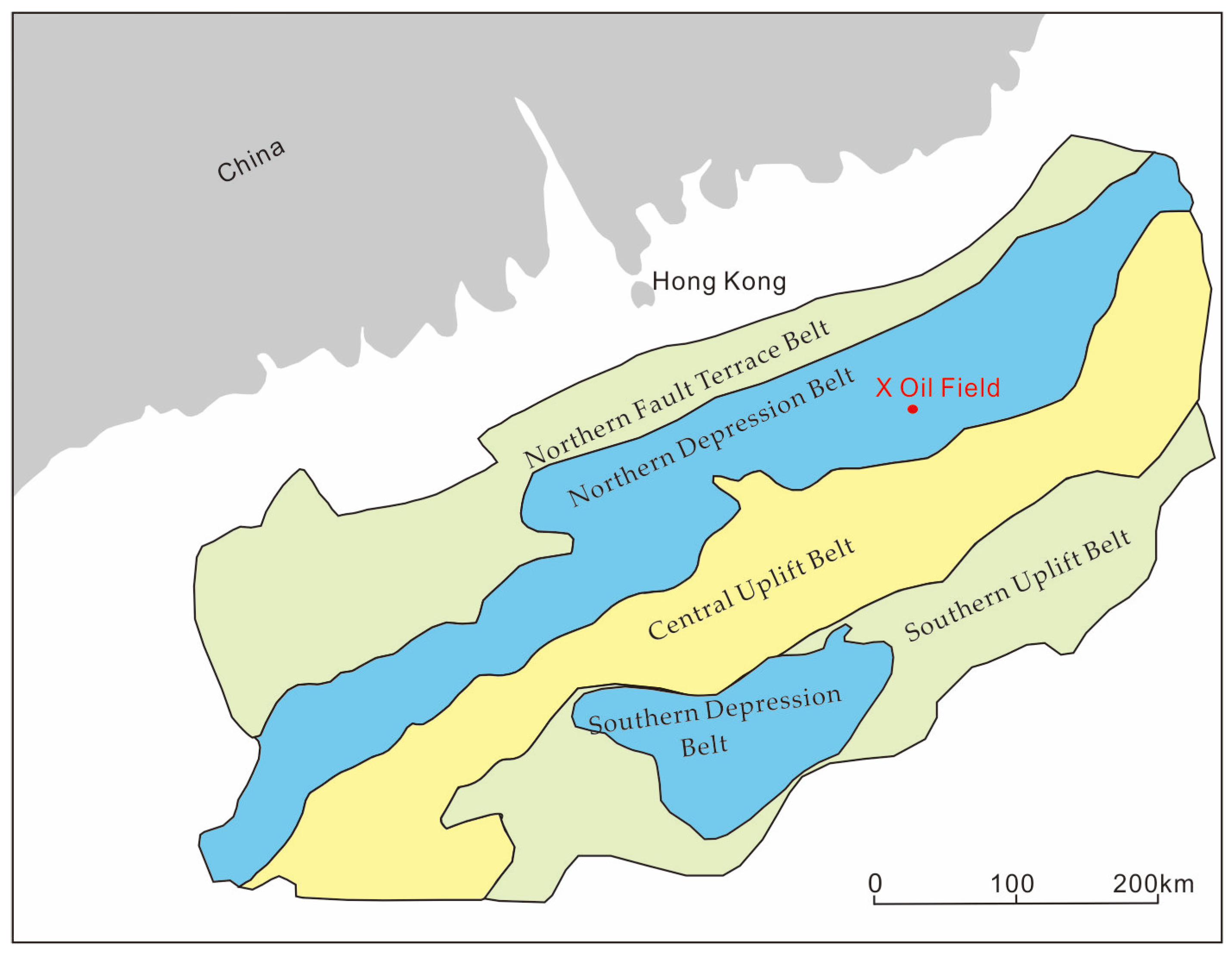
The Pearl River Mouth Basin is a continental margin rift basin formed during the Mesozoic–Cenozoic era. From north to south, it can be divided into five tectonic units: the Northern Fault Terrace Belt, the Northern Depression Belt, the Central Uplift Belt, the Southern Depression Belt, and the Southern Uplift Belt (Figure 1). The X Oilfield, which is the focus of this study, is located within the Zhu I Depression of the Northern Depression Belt and is a low-amplitude nose-shaped structure complicated by faults.

This basin exhibits the characteristics of “terrestrial origin followed by marine deposition” and “terrestrial source rocks with marine reservoirs” in its hydrocarbon accumulation assemblages. The Zhu-Qiong I Episode tectonic movement during the Early to Middle Eocene deposited semi-deep to deep lacustrine source rock series of the Wenchang Formation within the Zhu I Depression [12,13]. The Zhu-Qiong II Episode during the Middle Eocene led to the deposition of the lacustrine-swamp facies of the Enping Formation. Entering the Oligocene to Middle Miocene, under the background of widespread marine transgression, the reservoir rock series of the Zhujiang Formation, primarily consisting of deltaic to coastal clastic rocks, and the regional seal of the Hanjiang Formation sandstones and mudstones were deposited.

The Dongsha Movement from the end of the Middle Miocene to the end of the Late Miocene [14,15] was dominated by compressional detachment, facilitating the formation of numerous structural traps in the hanging walls within the Pearl River Mouth Basin. This period was also a critical stage for the final shaping of oil-bearing structures and the large-scale migration and accumulation of hydrocarbons [16].

X Oilfield is located in a Neogene sandstone reservoir in the Pearl River Mouth Basin of the South China Sea, with a structural relief of approximately 30 m. It is a low-amplitude anticlinal structure developed on basement uplift. The northern part of the oilfield is controlled by a set of en-echelon normal faults, and the sediment source is mainly from the northwest direction. The lateral variation in velocity is jointly influenced by the sediment source direction and fault structures, exhibiting a relatively pronounced trend.

Regional studies indicate that lateral velocity gradient variations are mainly controlled by two mechanisms: first, under the combined effects of vertical sedimentary compaction and lateral compression, the dehydration of mudstones near fault zones is more complete, leading to lateral changes in velocity; second, influenced by the sediment source direction, the percentage of sandstone and mudstone as well as porosity show distinct directional differences, which in turn cause lateral variations in velocity.

3. Materials and Method

In seismic exploration areas, factors such as near-surface structure, tectonic movement, burial depth of strata, and lateral variations in stratum thickness and lithology can all cause lateral variations in seismic wave propagation velocities [17,18]. Therefore, using a single velocity for time–depth conversion or conventional simple velocity variation mapping techniques often fails to accurately capture the lateral variation patterns of velocity, and cannot meet the precision requirements for structural mapping in the study area for oil and gas exploration and development. Taking X Oilfield as an example, this study proposes a set of velocity research methods and velocity variation mapping techniques suitable for low-amplitude structures, based on a systematic analysis of time–depth conversion issues.

3.1. Horizon Velocity Picking

Before conducting horizon-based velocity analysis, it is essential to perform detailed interpretation of the seismic data. The specific workflow is as follows:

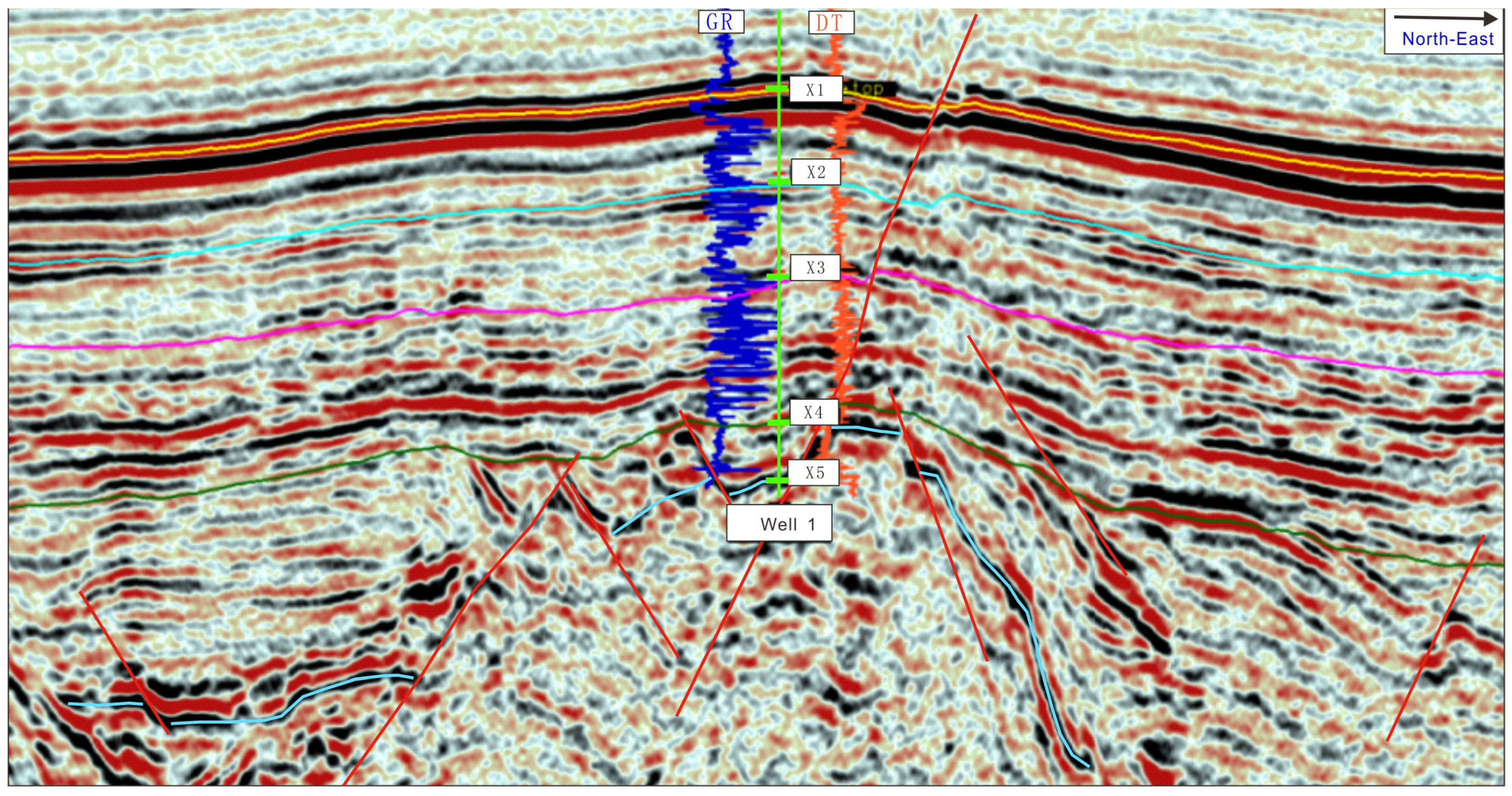
First, use Vertical Seismic Profile (VSP) data to calibrate the seismic horizons. VSP calibration is a key step in linking drilling geological information (depth domain) with surface seismic data (time domain). Its core lies in utilizing the precise “depth-time” correspondence provided by VSP to accurately map geological horizons (such as reservoir tops and bases, marker beds, etc.) onto the reflection events of seismic sections. Based on this, a unified well-seismic framework is established, and framework profile interpretation is carried out to determine the interpretation scheme.

Subsequently, based on the framework interpretation, a grid-based interpretation strategy with progressive refinement is adopted: initially, horizon tracking and correlation are performed over a large area using a relatively coarse grid (e.g., one control point per 16 lines × 16 traces) to establish a regional interpretation control network, ensuring preliminary closure of horizons over a broad area.

Then, the grid is further refined to a denser spacing (e.g., per 8 lines × 8 traces) to conduct systematic interpretation across the entire survey area. The focus at this stage is on achieving fine-scale closure of horizons and faults throughout the entire area, ensuring the consistency and reliability of the interpretation results in space.

Figure 2 displays the seismic calibration and interpretation profiles of geological horizons X1 to X5 in the X Oilfield.

The interval velocity is obtained using a high-precision velocity picking method and an integrated processing-interpretation approach based on along-layer velocity analysis, ensuring the rationality and accuracy of the velocity field in space. During the actual velocity analysis and picking process, the macro velocity field is first extracted in conjunction with the stacked sections corresponding to velocity control lines to ensure a smooth transition in velocity changes and minimize abrupt velocity variations in space. Subsequently, for the main target intervals, the data is processed with an enlarged scale. Based on the constraints of standard reference layers, seismic velocities are re-picked along the isochronous interfaces of the reservoirs to improve the accuracy of velocity interpretation. Ultimately, the density of the obtained 3D velocity field reaches 500 m × 500 m. 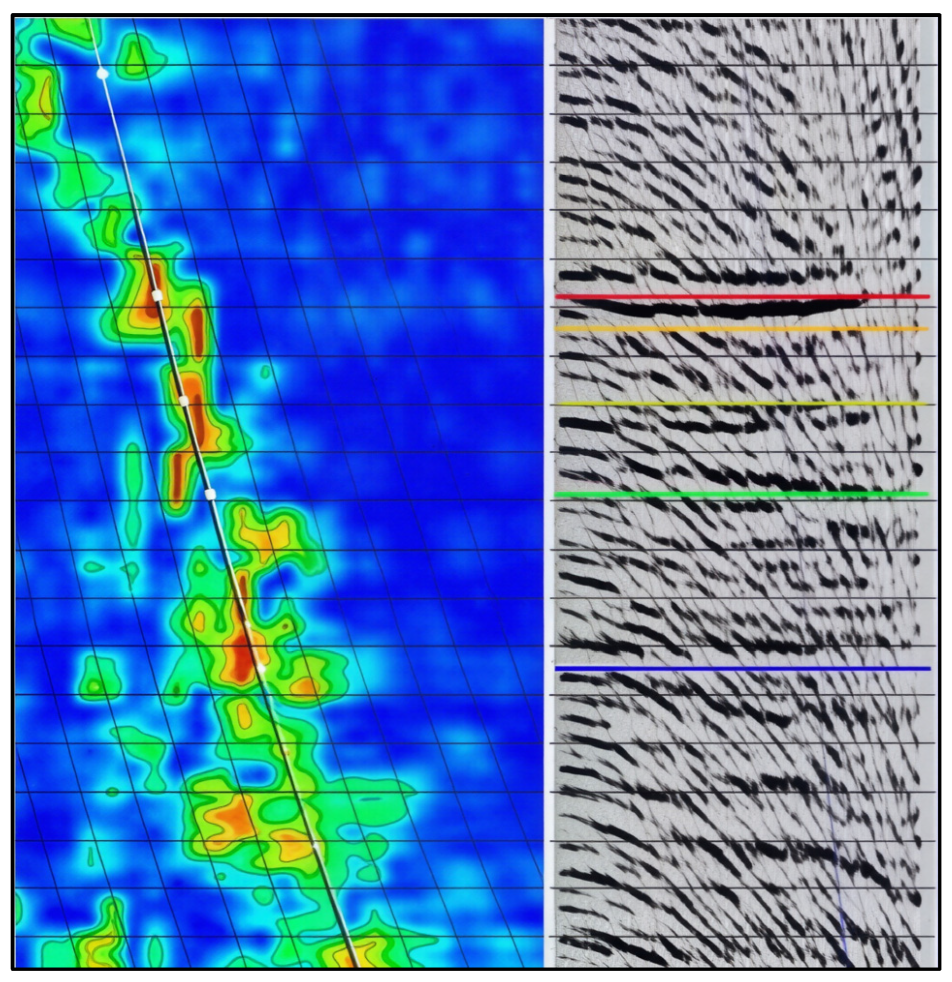Figure 3 shows an interpretation of the velocity spectrum. The colored lines in the figure represent the geological interpretation of the horizons.

This study fully leverages the advantages of integrated processing and interpretation. After obtaining a detailed velocity field, the first round of post-stack migration imaging processing is completed, followed by preliminary geological interpretation and evaluation. Subsequently, based on the horizon information provided by the geological interpretation, further along-layer velocity analysis is conducted to continuously enhance the accuracy of the velocity field.

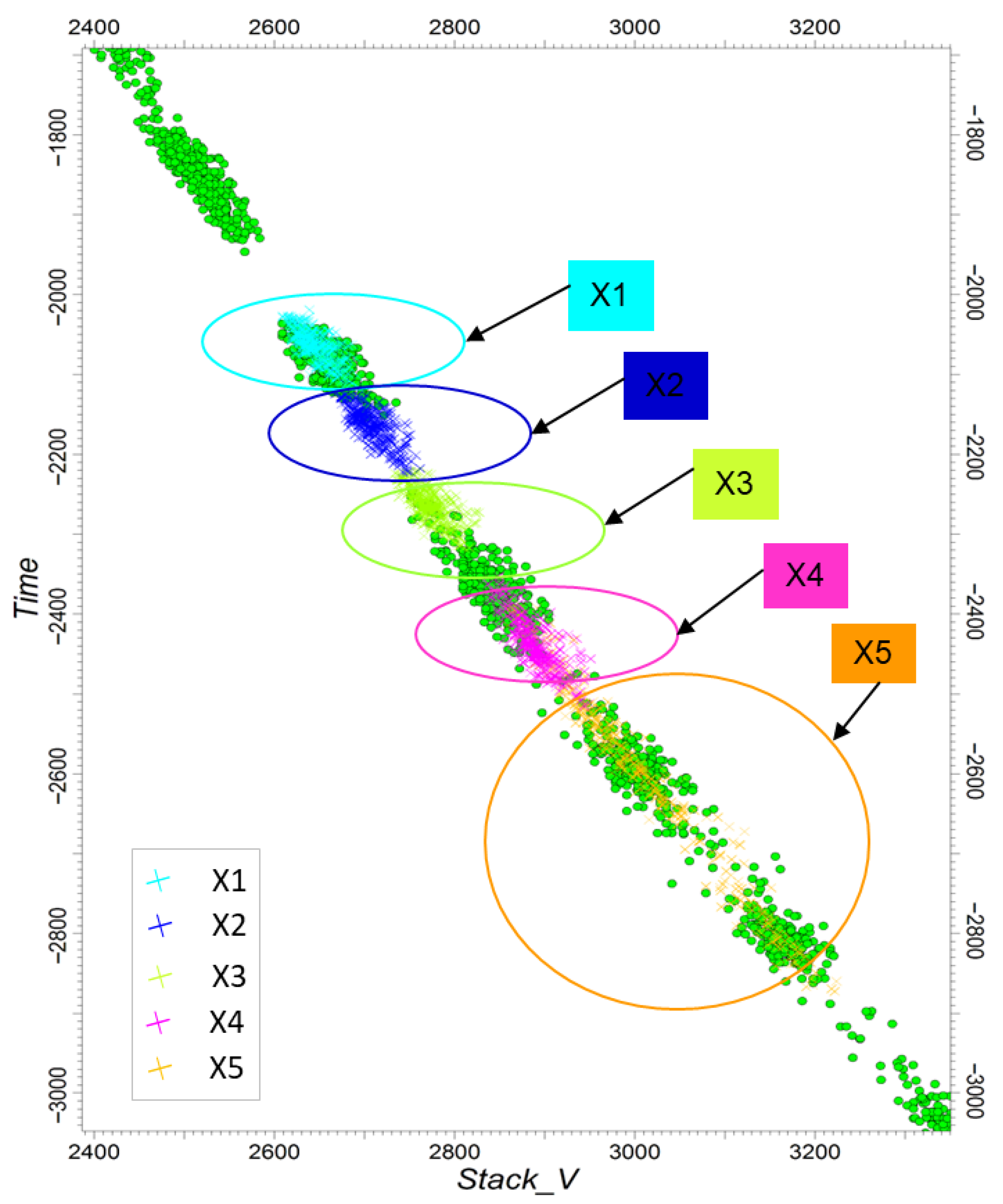
Figure 4 shows a scatter plot comparison between the horizon-based stacking velocities and the conventional stacking velocities. In the figure, the larger green circles represent conventional seismic velocity spectrum points, while the smaller colored cross points represent the horizon-based stacking velocity spectrum points. The comparison reveals that the scatter points of the conventional stacking velocities exhibit a wider distribution range in both time and velocity directions, with significantly greater dispersion than that of the horizon-based velocities, indicating that horizon-based velocity picking achieves higher accuracy.

3.2. Establishment of Average Velocity Field

After completing the seismic velocity picking along the reservoir isochronous interface, it is necessary to further calculate the average velocity. First, dip angle information of the reservoir isochronous interface is obtained through horizon tracking. Based on this, model tomography processing is carried out using GeoEast software(V3.0). For example, after completing the seismic interpretation and horizon-velocity picking of interface X1, import the interpreted horizon X1 and its horizon-velocity points into GeoEast software. Set the maximum number of iterations to 10 and use interface X1 and its corresponding horizon velocity as the initial model. Based on ray-tracing forward modeling and actual seismic travel-time inversion fitting, the software finally obtains the horizon velocity field of the X1-X2 interval after 8 iterations.

This method takes the known interval velocity and reflection interface of the (n − 1) th layer as input. According to the principles of curved-ray tracing and the geometric relationship that the angle of incidence equals the angle of reflection, the interval velocity of the nth layer is calculated layer by layer through 5–15 iterations, and the nth reflection interface is determined. Simultaneously, the offset position of the reflection point relative to the incident point is updated. By recursively processing layer by layer, a seismic velocity field covering the entire work area is ultimately established. 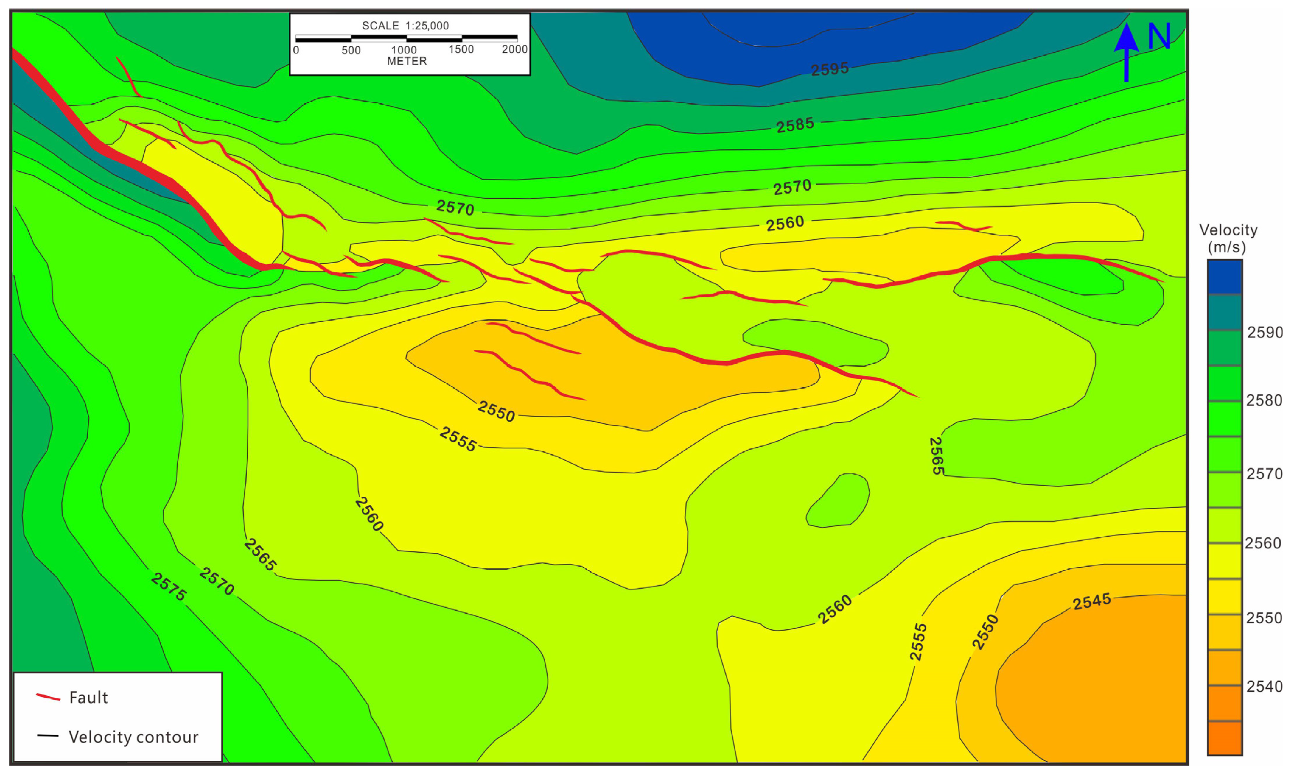Figure 5 illustrates the initial average velocity planar distribution of the target layer in the X Oilfield. The spatial pattern of this velocity distribution shows good consistency with the morphology of the time structure T0 map.

3.3. Macro Velocity Trend Correction

Based on the interpretation of a standard reference horizon from time-domain seismic data and depth-domain well log information, assuming that the relative isochronal interfaces in the time domain and the corresponding depth-domain well log horizons satisfy the probability distribution characteristics of spatial time–depth conversion velocities, when the following expression is minimized, the fitting coefficients $v_0$ and β for the average time–depth conversion velocity between the time-domain seismic horizon and the depth-domain well log horizon (such as the top, bottom, or other adjacent layers of the reservoir near the well) can be determined.

$${\displaystyle \sum _{j=1}^M}{\displaystyle \sum _{i=1}^n}{\left[\left({\displaystyle \frac{2z_i}{t_i}}\right)-v_0(1+\beta z_i)\right]}^2$$

$t_i$: Two-way travel time of the seismic horizon near the well;

$z_i$: Depth of the drilling formation layer;

$i$: The number of logging points;

$j$: The number of reference layers;

$v_0$: The fitted reservoir top velocity;

β: The coefficient varying with depth.

Using the above formula and solving for the minimum of the objective function via the interior-point constrained optimization algorithm, the fitting coefficients $v_0$ and β of the average time–depth conversion velocity can be obtained, thereby establishing the well side average velocity fitting function. Based on this well-seismic fitted average velocity curve, a macroscopic trend correction can be applied to the seismic velocity field. 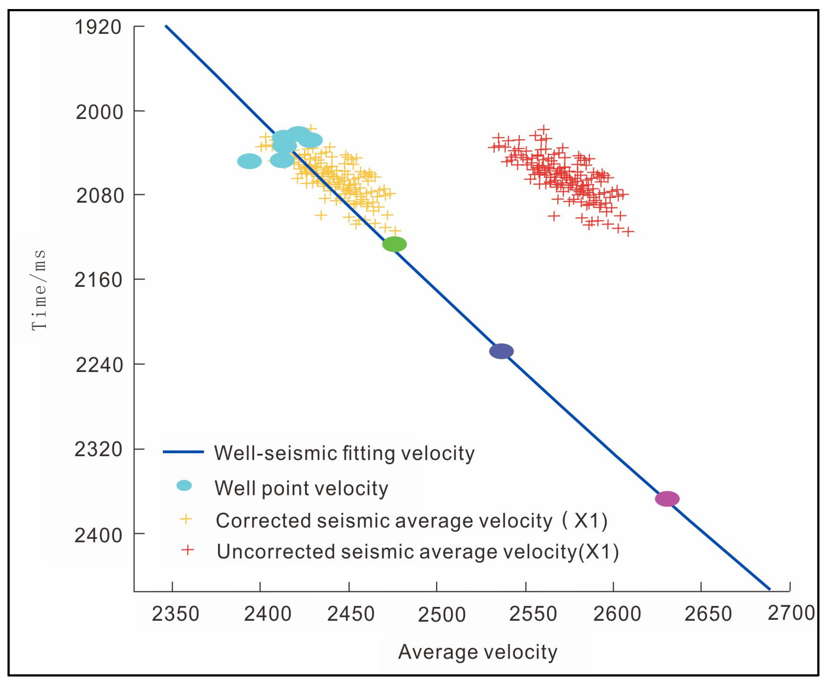Figure 6 shows a comparison of the seismic average velocity before and after correction for layer X1. It can be observed that there is a certain trend difference between the seismic velocity field and the fitted velocity. This difference, typically caused by factors such as VTI anisotropy, is commonly present between seismic and logging velocities, making it necessary to perform macroscopic velocity trend correction. 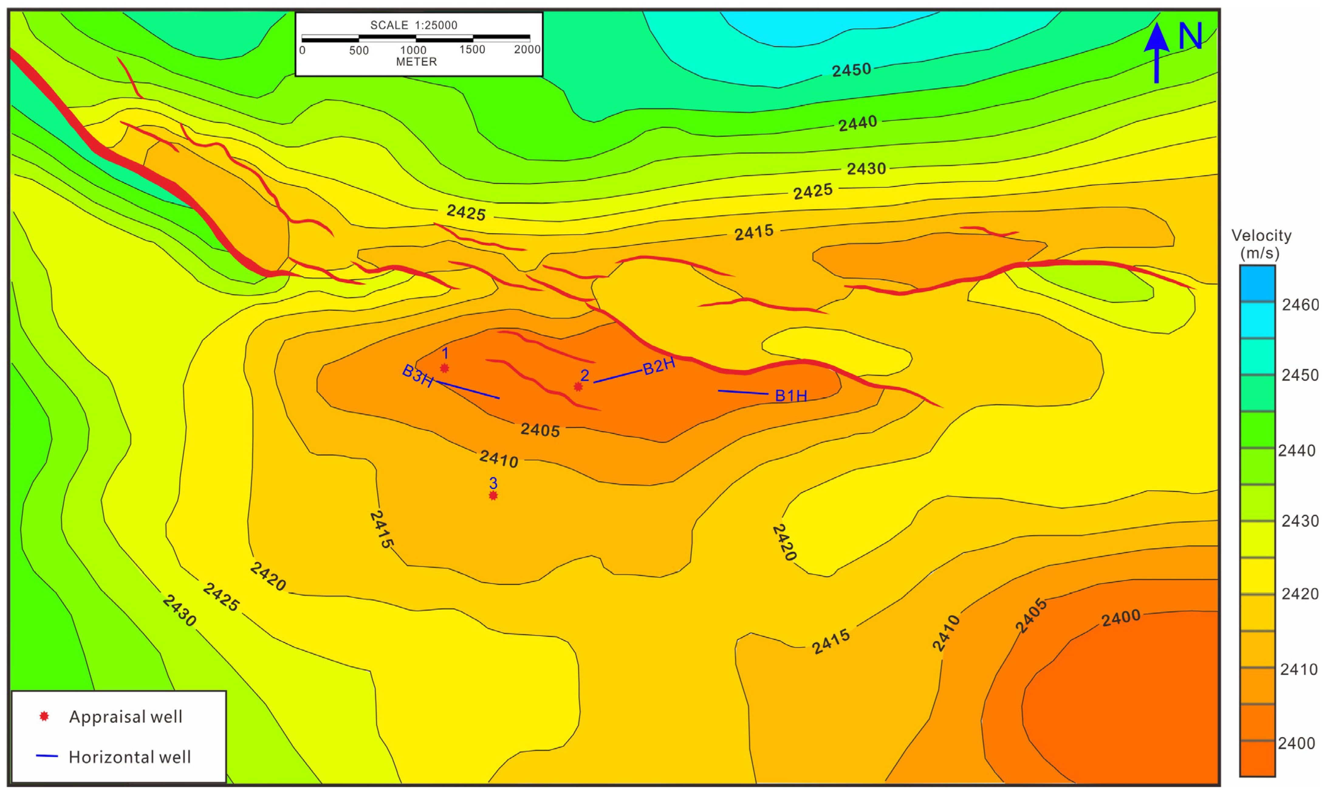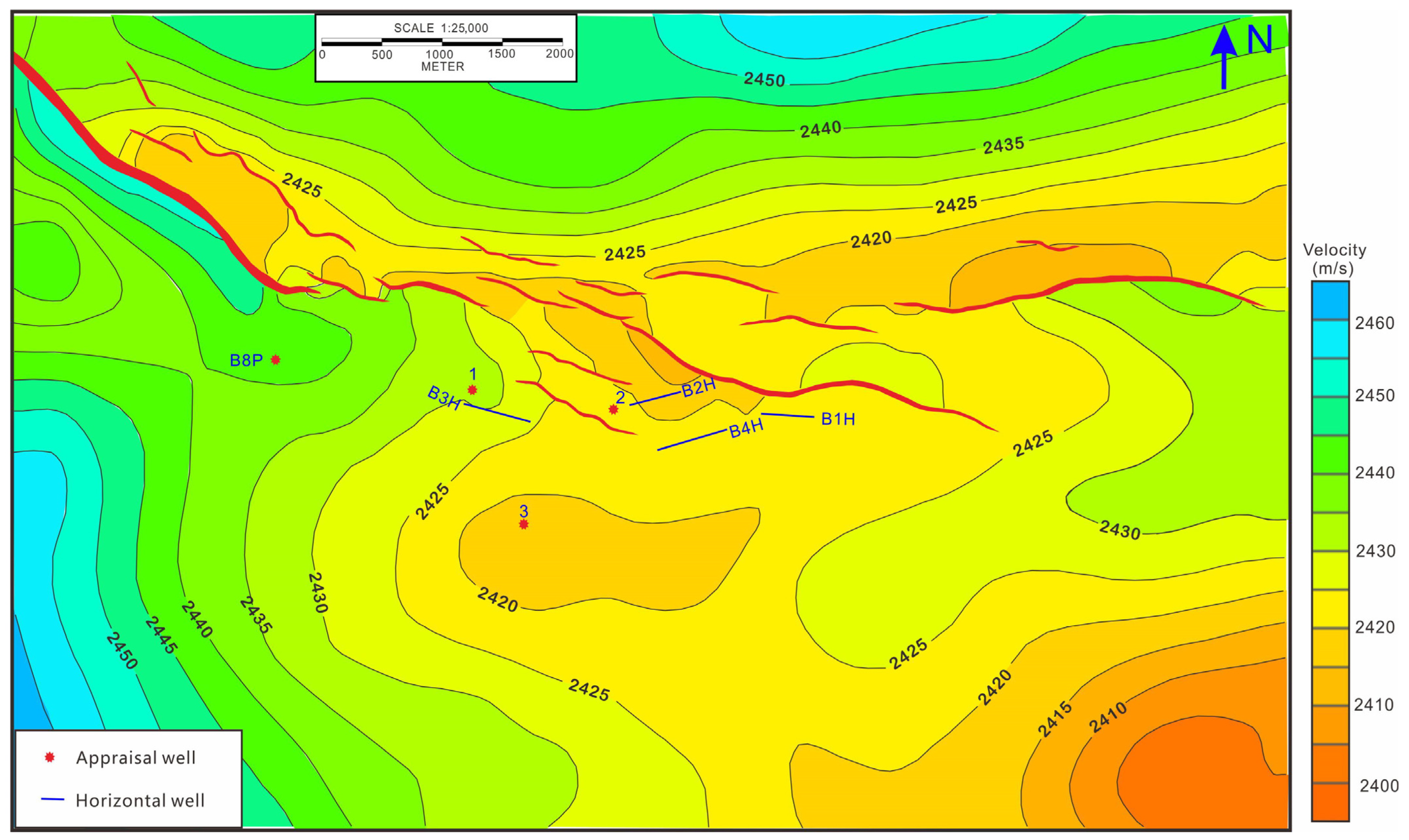Figure 7 displays the planar distribution characteristics of the average velocity along the layer after macroscopic trend correction. Compared with the pre-correction velocity map (Figure 5), the two are largely consistent in planar morphology, differing only in numerical trends, with an overall difference of approximately 145 m per second.

3.4. Spatial Residual Factor Correction of Well-to-Seismic Data

As shown in Figure 6, there is still a certain deviation between the seismically derived average velocity after macro-trend correction and the fitted velocity curve. Therefore, further well-to-seismic spatial residual factor correction is required. The specific correction steps are as follows:

(1)

On the interpreted time structure map of the target horizon, extract the reflection time values corresponding to all well points (including the entry and exit points of drilled horizontal wells) to obtain the two-way reflection times at each well point; divide this time by 2 to obtain the one-way reflection time at each well point.

(2)

Calculate the actual average velocity at each well point by dividing the actual drilling depth by its one-way reflection time (

Table 1. Relationship between well point time, depth, and velocity.

Well Name	Two-Way Reflection Time (TWT: s)	One-Way Reflection Time (OWT: s)	Drilling Depth (m)	Velocity (m/s)
1	2.0293	1.0146	2461.6	2426.1
2	2.0290	1.0145	2450.4	2415.3
3	2.0440	1.0220	2468.4	2415.3
B1H1	2.0301	1.0150	2453.4	2417.0
B1H2	2.0334	1.0167	2458.6	2418.2
B2H1	2.0272	1.0136	2449.6	2416.8
B2H2	2.0259	1.0129	2444.0	2412.8
B3H1	2.0286	1.0143	2455.5	2420.9
B3H2	2.0300	1.0150	2461.2	2424.8
B4H1	2.0325	1.0163	2457.1	2417.8

).

(3)

Based on the actual average velocities at all drilled well points (including the entry and exit points of horizontal wells), perform well-point-constrained correction on the average velocity map after macro-trend correction. Figure 8 shows the average velocity map of the target horizon after well-to-seismic spatial residual factor correction.

3.5. Time-to-Depth Conversion and Structural Mapping

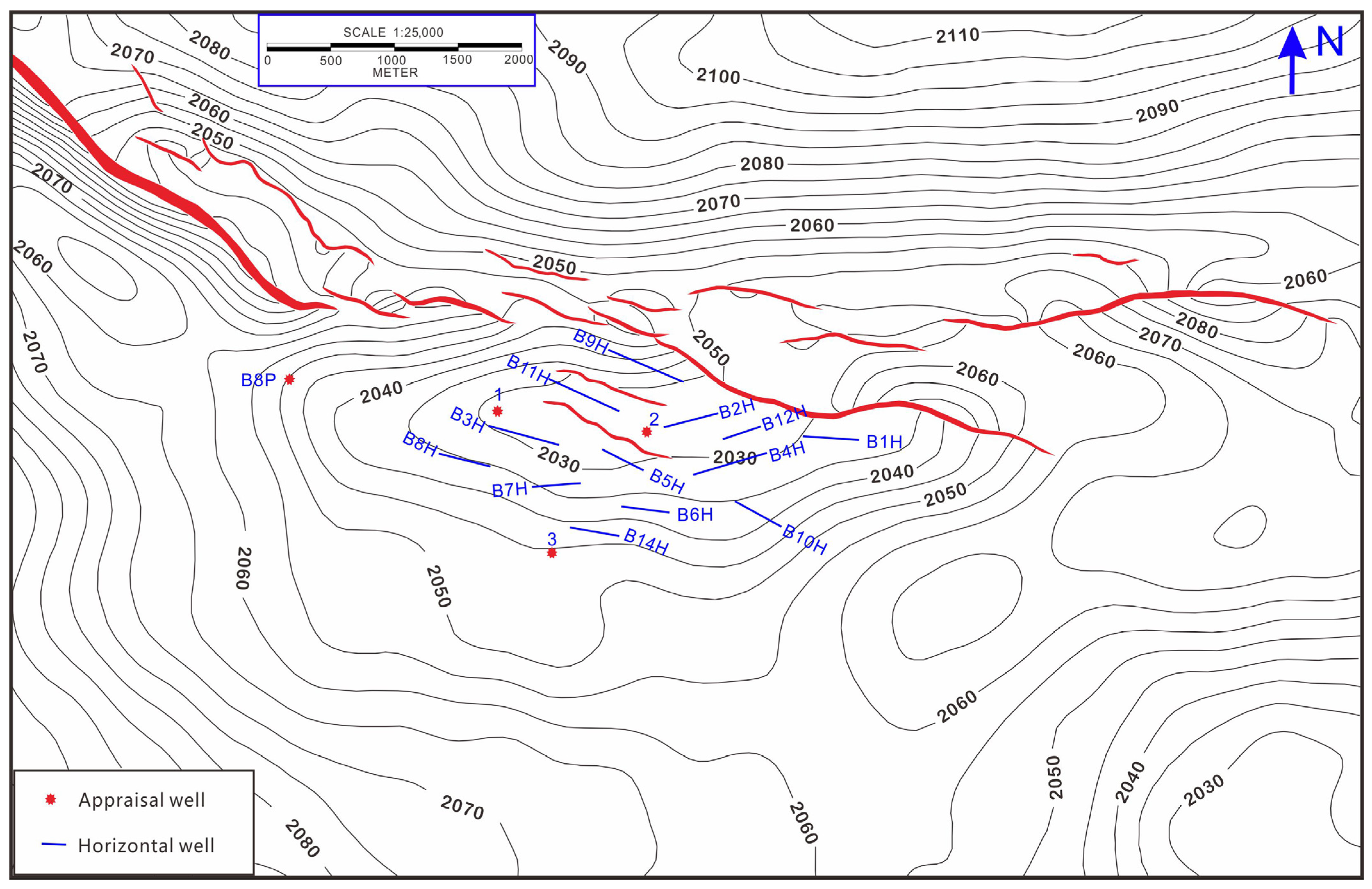
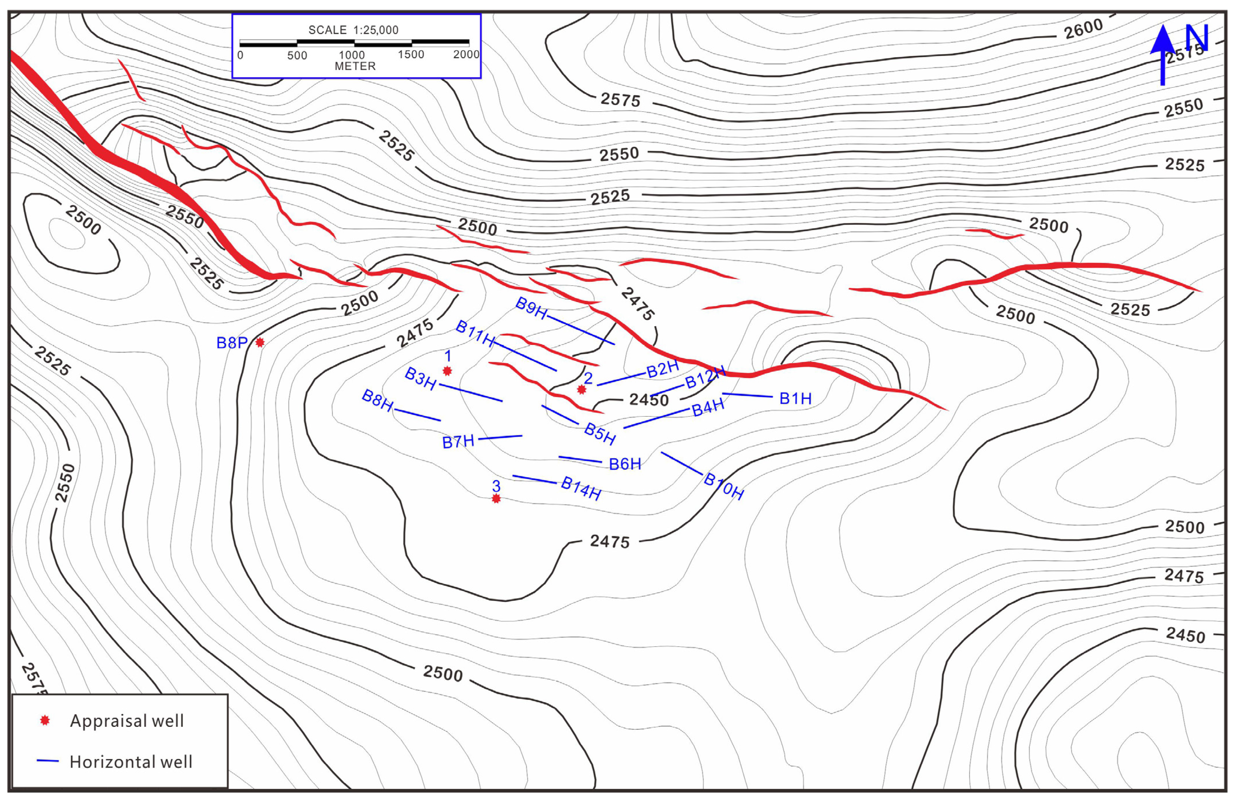
Based on the time structure map (isochronous T0 map, Figure 9) of the target horizon obtained from 3D seismic data interpretation, we first divide its time values by 2 to obtain a planar distribution map reflecting the one-way reflection time of this horizon. Subsequently, this one-way reflection time map is multiplied point-by-point with the average velocity map of the target horizon (Figure 8), which has been corrected for well-seismic spatial residual factors, to finally complete the time-to-depth conversion and generate a high-precision depth structure map of the target horizon (Figure 10).

The mathematical expression of this process can be simplified as:

Depth Structure Map = (Target Horizon Isochronous T0 Map/2) × Target Horizon Average Velocity Map of the Layer.

This conversion physically corresponds to the relationship between two-way travel time and average velocity under the condition of seismic wave normal incidence, i.e., the depth of the target horizon equals the product of its one-way reflection time and velocity. Through this mapping, seismic information in the time domain is transformed into the structural morphology in the geological depth domain, providing a crucial depth framework for subsequent reservoir characterization, well placement, and detailed evaluation of hydrocarbon reservoirs.

4. Results

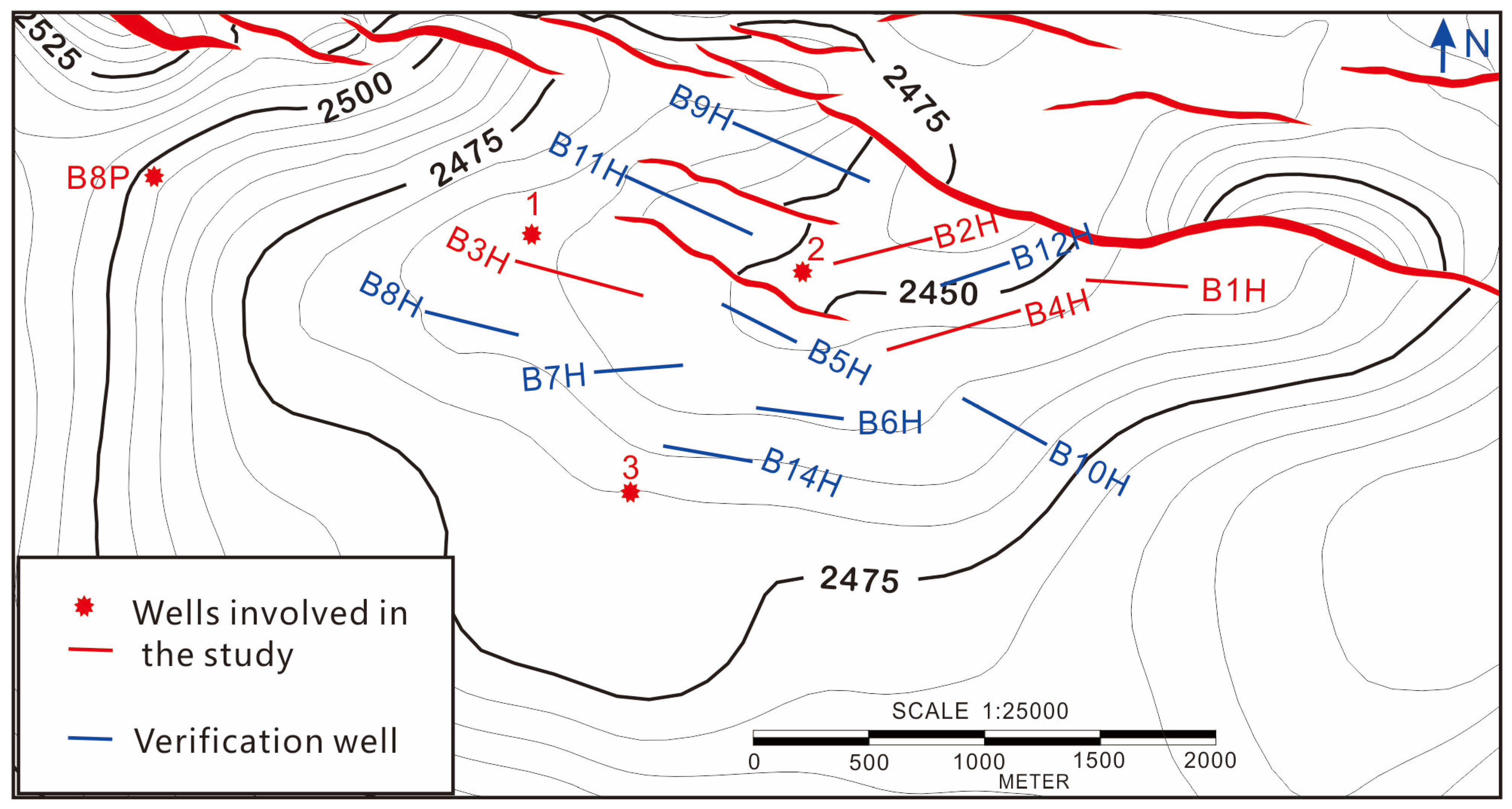
The structural map established through detailed velocity research has been well validated and applied in subsequent drilling practices. Figure 11 shows a local enlargement of the depth structure of the X1 layer at well locations, where red markers indicate wells involved in the preliminary study, and blue markers indicate verification wells drilled later. Actual drilling results show that the error between the drilling depth of the verification wells and the predicted depth is controlled within 3 m, with the actual encountered depth of most wells differing from the model predictions by only about 1 m, demonstrating a high degree of consistency and prediction accuracy.

To further systematically evaluate the structural prediction accuracy of the well-seismic joint velocity mapping method, this study also employed the conventional along-layer time–depth relationship method for comparative analysis. This method is based on the actual well depth at the target horizon and the corresponding seismic interpretation time values, fitting an along-layer time–depth relationship equation to complete the time–depth conversion and structural mapping.

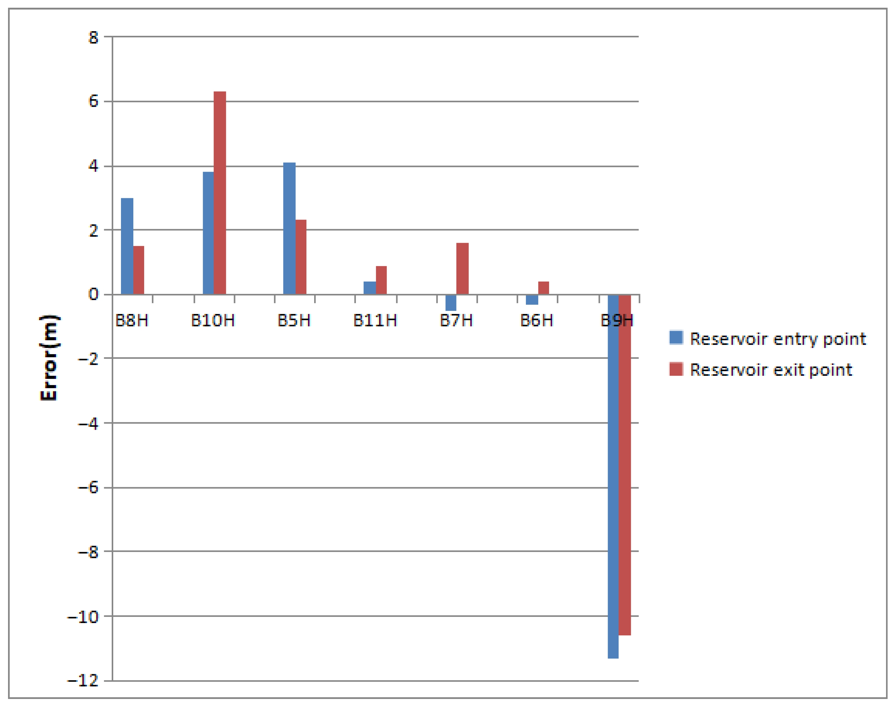
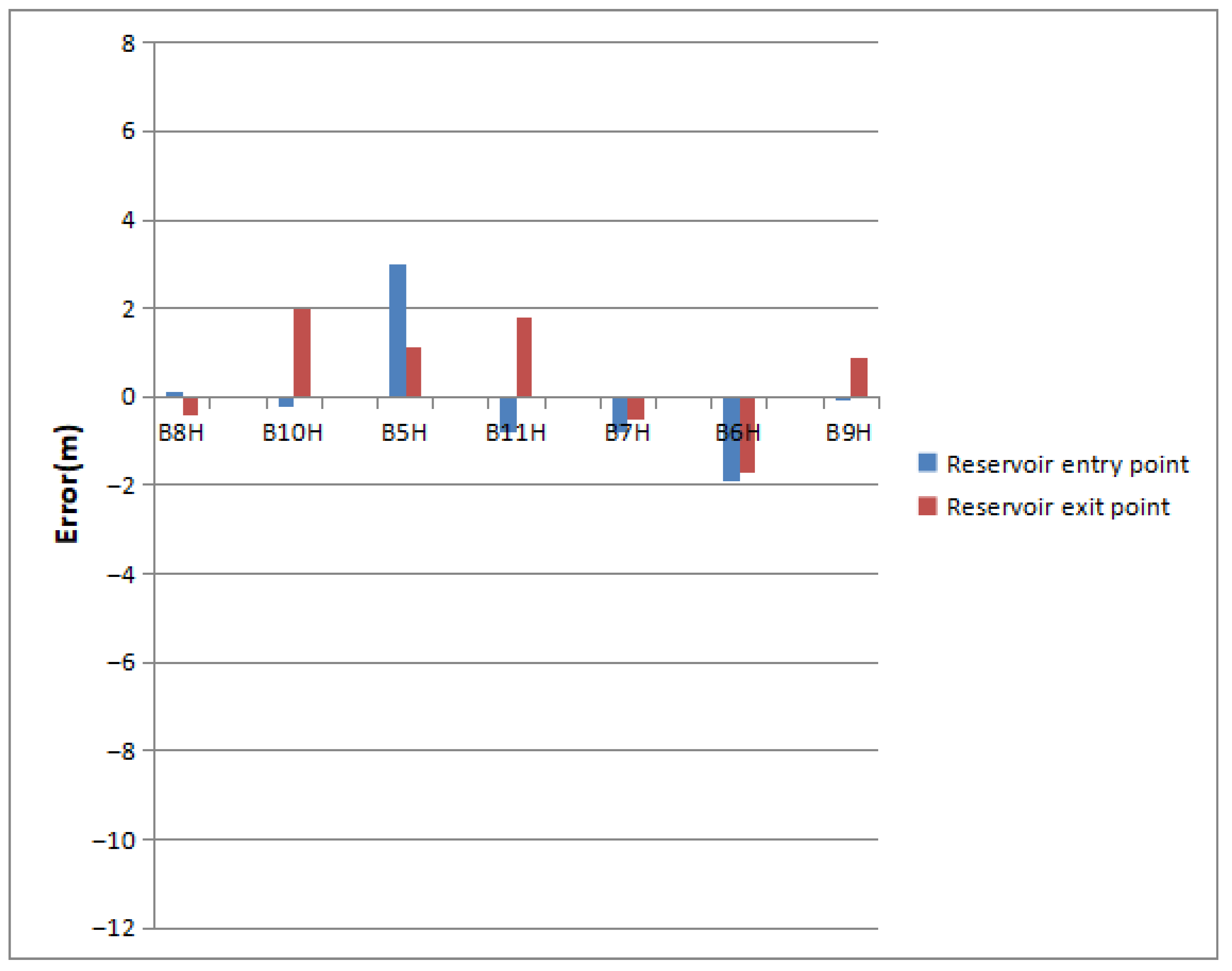
From the comparison results of the actual drilling depth and predicted depth errors in the oilfield (Figure 12 and Figure 13), it can be seen that in the main area of the oilfield, the structural prediction errors of both the along-layer time–depth relationship method and the well-seismic joint velocity method are small, with the two showing good consistency. However, in the edge areas of the oilfield, specifically near the B10H and B9H wells, the error of the structural map converted using the along-layer time–depth relationship method increases significantly, while the well-seismic joint velocity method still maintains high prediction accuracy, demonstrating stronger adaptability and reliability. It is important to emphasize that these two key wells located at the structural edge have a crucial impact on accurately evaluating the development potential of the oilfield, optimizing well pattern deployment, and supporting the formulation and implementation of overall adjustment and development plans. The accuracy advantage of the well-seismic joint velocity method in the edge areas further highlights its practical value in fine structural characterization during the middle and late stages of oilfield development, providing solid geological basis and decision-making support for rolling exploration and development.

This achievement not only validates the effectiveness and reliability of the velocity research method but also lays a scientific foundation for subsequent well location deployment, drilling risk control, and efficient reservoir development. It contributes to improving overall development efficiency and promotes more precise and efficient management and development of the oilfield.

5. Discussion

From the velocity distribution characteristics of the X1 reservoir (Figure 8), significant lateral velocity gradient variations are observed both parallel and perpendicular to the fault direction. Well velocity data indicate that in the direction parallel to the faults, velocity increases with depth from the structural high to the west and east, consistent with the general velocity variation pattern under sedimentary compaction. Specifically, the structural high exhibits lower velocity due to shallower burial and relatively lower compaction, while the structural flanks show higher velocity due to increased burial depth and enhanced compaction. Additionally, controlled by the northwest sediment source, the sandstone-to-mudstone ratio and lithological combination vary laterally, resulting in a significantly greater velocity increase in the west compared to the east. This reflects the significant influence of the sediment source-depositional system on the velocity field.

In the direction perpendicular to the faults, the average velocity at Well 3, located on the structural flank, is lower than that at Well 2 on the structural high, exhibiting a velocity reversal phenomenon contrary to the conventional compaction trend. This anomalous feature is primarily controlled by diagenetic modifications and stress distribution related to fault activity: areas closer to the faults experience more complete mudstone dehydration, resulting in tighter rock grain contacts and relatively higher velocities. In contrast, areas farther from the faults undergo weaker diagenesis, with relatively preserved pore structures and lower velocities. This distribution pattern exhibits typical fault-controlled lateral velocity gradient characteristics, reflecting the profound impact of tectonic activity on reservoir properties and the velocity field.

The aforementioned velocity distribution patterns have important implications for seismic data processing, time–depth conversion, and structural interpretation. Particularly in the context of low-amplitude structures, accurate characterization of lateral velocity variations is crucial for delineating structural morphology, assessing trap effectiveness, and optimizing well placement.

6. Conclusions and Future Development

(1)

The well-seismic integrated time–depth conversion technology can significantly improve the prediction accuracy of structural maps, making it particularly suitable for the fine-scale structural characterization and evaluation during the middle and late stages of oilfield development. By effectively integrating drilling depth and seismic time information, this technology markedly reduces the error between actual drilled depth and predicted depth, providing reliable geological evidence for well placement and adjustment decisions in the oilfield development phase.

(2)

The root cause of prediction errors for low-amplitude structures lies in the lateral heterogeneity of the velocity field, which leads to asymmetry in the travel times of seismic waves during their downward and upward propagation paths. Therefore, to fundamentally enhance the imaging and interpretation accuracy of such structures, it is necessary to further conduct high-precision pre-stack depth migration and imaging processing or employ pre-stack time migration methods based on asymmetric travel time theory, in order to more accurately describe the impact of lateral velocity variations on wave propagation paths.

(3)

In the future, emerging technologies such as full waveform inversion and artificial intelligence velocity modeling can be integrated to establish higher-resolution velocity models. Additionally, research on the synergistic mechanisms of well and seismic data in time–depth conversion should be deepened. This will better serve the fine-scale development of complex hydrocarbon reservoirs and the tapping of remaining oil potential.

References

- Wang, J.; Zhang, S.; Du, W.; Li, L.; Qiao, Z.; Zhang, J.; Duan, M. The control effect of low-amplitude structure on oil-gas-water enrichment and development performance of ultra-low permeability reservoirs. Pet. Explor. Dev. Online 2019, 46, 767–778. [Google Scholar] [CrossRef]
- Guo, A.; Lu, P.; Zhang, X.; Chen, X.; Jiang, S.; Wang, B. Identification methods for low-amplitude structures in Oilfield A. J. Geophys. Eng. 2025, 23, 373–384. [Google Scholar] [CrossRef]
- Lyu, F.; Liu, Y.X.; Chen, L.; Li, C.; Zhou, J.; Zhou, H.L. Low-amplitude structure recognition method based on non-subsampled contour-let transform. Pet. Sci. 2024, 21, 3062–3078. [Google Scholar] [CrossRef]
- Su, C.; Xu, H.; Zhong, D.; Zhang, B.; Jiang, T.; Yang, J.; Ju, B. Low relief structure interpretation and mapping of the Donghe Sandstone thin reservoir based on seismic data. J. Pet. Sci. Eng. 2020, 195, 107945. [Google Scholar] [CrossRef]
- Li, B. The Study and Application of Low Relief Structure Interpretation and Mapping. IOP Conf. Ser. Earth Environ. Sci. 2018, 170, 022031. [Google Scholar] [CrossRef]
- Wang, J.; Wang, J. Low-amplitude structures and oil-gas enrichment on the Yishaan Slope, Ordos Basin. Pet. Explor. Dev. Online 2013, 40, 52–60. [Google Scholar] [CrossRef]
- Bambang, J.I.; Wahyu, T. 3D Check shot Modeling for Time-Depth Conversion. IOP Conf. Ser. Earth Environ. Sci. 2023, 1227, 012018. [Google Scholar] [CrossRef]
- Al-Khazraji, O.N. Cross-validation of time-depth conversion and evaluation of different approaches in the Mesopotamian Basin, Iraq. Explor. Geophys. 2023, 54, 288–315. [Google Scholar] [CrossRef]
- Qadir, A.; Chizzini, N.; Maiorana, M.; Artoni, A.; Torelli, L.; Sulli, A. Velocity Model Construction and Time-to-Depth Conversion of a Vintage Seismic Reflection Profile for Improving the Constraints on a Subsurface Geological Model: An Example from the Sicily Channel (Central Mediterranean Sea). Geosciences 2025, 15, 114. [Google Scholar] [CrossRef]
- Xie, Q.; Fan, H.; Chen, J.; Rui, Z.; Wu, C.; Tong, Y. An integrated velocity model application in ST area, Dongying Depression, China. Acta Geophys. 2023, 72, 141–159. [Google Scholar] [CrossRef]
- Kulikowski, D.; Hochwald, C.; Amrouch, K. An automated cross-validation method to assess seismic time-to-depth conversion accuracy: A case study on the Cooper and Eromanga basins, Australia. Geophys. Prospect. 2018, 66, 1521–1534. [Google Scholar] [CrossRef]
- Li, W.; Cao, M.; Meng, M.; Fan, C.; Li, H.; Li, J.; Wu, W.; Qin, R.; Li, X.; Liu, Y. Characteristics of transfer zones under the influence of pre-existing faults and regional stress transformation: Wenchang A subsag, Zhujiang River Mouth Basin, northern South China Sea. J. Oceanol. Limnol. 2024, 42, 744–759. [Google Scholar] [CrossRef]
- Fu, X.; Chen, S.; Lu, J.; Lei, M. Geochemical characteristics and origin of crude oil and natural gas in different areas of Wenchang-A Sag, Pearl River Mouth Basin, South China Sea. Front. Earth Sci. 2024, 18, 714–731. [Google Scholar] [CrossRef]
- Cheng, H.; Suo, Y.; Zhu, D.; Li, S.; Zhou, J.; Wang, P.; Du, X.; Wang, G. Cenozoic Tectonothermal History of the Pearl River Mouth Basin, Northern South China Sea: Insights from Fission Track and Seismic Data. J. Ocean Univ. China 2026, 25, 171–183. [Google Scholar] [CrossRef]
- Tang, X.Y.; Yang, S.C.; Hu, S.B. Tectonic-thermal history and hydrocarbon potential of the Pearl River Mouth Basin, northern South China Sea: Insights from borehole apatite fission-track thermochronology. China Geol. 2023, 6, 429–442. [Google Scholar] [CrossRef]
- Jiang, H.; Pang, X.; Shi, H.; Liu, L.; Bai, J.; Zou, S. Effects of fault activities on hydrocarbon migration and accumulation in the Zhu I Depression, Pearl River Mouth Basin, South China Sea. Aust. J. Earth Sci. 2015, 62, 775–788. [Google Scholar]
- Persico, R.; Morelli, G.; Esposito, G.; Catapano, I.; Capozzoli, L.; De Martino, G.; Yang, D. An innovative time-depth conversion for the management of buried scenarios with strong discontinuities. J. Appl. Geophys. 2024, 227, 105435. [Google Scholar] [CrossRef]
- Yang, D.; Capozzoli, L.; Catapano, I.; Martino, G.D.; Esposito, G.; Morelli, G.; Persico, R. Accounting for the Different Propagation Velocities for the Focusing and Time–Depth Conversion in a Layered Medium. Appl. Sci. 2024, 14, 11812. [Google Scholar] [CrossRef]