A Discrete-Time FOLQR Framework for Centralized AGC in Multi-Area Interconnected Power Grids

Abstract

This paper presents a discrete-time, centralized fractional-order linear quadratic regulator FOLQR for automatic generation control (AGC) of three-area interconnected nonreheat thermal systems. The AGC state explicitly includes the area control error (ACE) and tie-line power; a quadratic performance index penalizes ACE, its integral (IACE), and control effort. The continuous-time plant (governor–turbine dynamics and tie-line flows) is discretized at a fixed sampling interval, and a single centralized gain is obtained from the discrete algebraic Riccati equation; the fractional-order extension shapes memory in the feedback to temper rapid transients. Benchmark studies under 0.01 and 0.05 p.u. step-load disturbances show that FOLQR stabilizes the interconnection and consistently lowers peak excursions relative to a conventional discrete LQR (COQAGC) baseline—reducing frequency peaks by about 9–12% and tie-line peaks by 24–60% in the small-step case—while producing smoother actuator commands. Although FOLQR exhibits longer settling times, this trade-off is acceptable FOr multi-area AGC where limiting overshoot and tie-line excursions is operationally more critical than strict settling-time targets. The proposed controller retains a simple centralized, discrete-time structure with a modest computational burden, making it suitable FOr real-time AGC deployment in large interconnected grids and demonstrating for the first time, to our knowledge, a fractional-order LQR applied to a three-area thermal benchmark.

1. Introduction

Automatic generation control (AGC) has long been recognized as essential for maintaining system stability [1] and for improving the dynamic and transient performance of interconnected multi-area power grids. With increasing renewable penetration, challenges such as frequency regulation [2], tie-line scheduling, and disturbance mitigation have intensified, motivating advanced control architectures and optimization driven strategies. Recently, metaheuristic and soft computing methods have attracted significant attention for enhancing AGC performance under high renewable integration [3]. A wide range of AGC strategies has been proposed. Representative examples include fractional-order controllers such as FOPIλD [4], classical linear techniques [5,6], intelligent frameworks such as ANFIS-based neuro-fuzzy systems [7,8], variable-structure control [9], active disturbance rejection control (ADRC) [10], and robust $H_{\infty }$ designs [11]. In multi-area settings with hydro/thermal plants and distributed energy resources, advanced schemes, e.g., brain emotional learning with fractional calculus (FOBELBIC), have been employed to reduce frequency excursions and tie-line deviations [12]. Hybrid intelligent FOPID controllers with type-2 fuzzy logic likewise aim to suppress oscillations and power variations in disturbed two-area systems [13]. However, most designs are formulated in continuous time, whereas practical deployments use discrete-time control to accommodate digital sampling [14]. Ignoring sampling effects can degrade stability and performance [15], underscoring the need for discrete-time AGC strategies that explicitly capture sampled-data behavior.

Modern optimal control approaches especially LQR have been widely studied for robustness to load variations, model uncertainty, and constraints. Early works emphasized two-area systems [16,17]; LQR performance depends critically on the weighting matrices Q and R [18,19]: The weighting matrix Q and R [20] Reported matrix selection approaches include identity choices [21,22], participation-factor analysis [23], BFO–PSO hybrid optimization more recent efforts include bacteria foraging oriented PSO combined with LQR to handle nonlinearities and parameter variations [24], with extensions to interconnected microgrids [3,19]. Larger R curbs control effort at the cost of responsiveness, whereas larger Q penalizes state deviations more strongly [24] and eigenvalue-based methods [25]. Many of these require observers; in contrast, the functional minimization method (FMM) can avoid full-state observation by leveraging ACE fluctuations, their integrals, and control-signal variations [25,26], making it attractive for discrete-time AGC with communication delays.Beyond LQR, several advanced and hybrid controllers have been explored. Lalngaihawma et al. [27] proposed TIDN tuned via zebra optimization, and Kumar and Prasad [28] developed a CFPIDF–PI controller for hybrid hydrothermal systems. Other works compared firefly optimized and PD–PID designs [29,30]; Machine learning approaches such as reinforcement learning and neural networks have been investigated [31], Gray Wolf Optimization has also been applied to improve damping in deregulated grids [32] though they typically lack an explicit LQR formulation. GA–PSO hybrids are common for PID/FOPID tuning [33,34,35], and type-2 fuzzy controllers address uncertainty and nonlinearity [36,37]. In parallel, deregulated market frameworks and area-error analysis [38] highlight the role of devices such as TCPS and storage in AGC design.

More recently, Esmail and Krishnamurthy [39] proposed a centralized discrete-time AGC based on LQR cost minimization; and Abdo et al. [40] used TVAC–PSO for PID tuning in isolated plants. Collectively, these studies point to discrete-time, centralized frameworks as a promising path to computationally efficient, high-performance AGC for modern interconnected power systems. Singh et al. [41] introduced a rank-exponent method benchmarked against LQR.

Recent studies have explored advanced optimal and intelligent control strategies to enhance Automatic Generation Control (AGC) performance. Fractional-order optimal control was introduced in [42], where a fractional-order linear quadratic regulator demonstrated improved robustness and tuning flexibility compared to classical LQR methods. Intelligent control techniques were further investigated in [43] using fuzzy gain scheduling controllers to address nonlinearities and parameter variations in two-area interconnected power systems. Optimization-based AGC design was presented in [44], where a teaching learning based optimization algorithm was applied to multi-area systems with diverse energy sources, yielding improved dynamic performance. More recently, a discrete optimal quadratic AGC framework based on cost functional minimization was proposed in [45], highlighting the effectiveness of optimal control strategies for interconnected power systems.

Cybersecurity-aware and communication-efficient AGC has recently emerged as a key research direction, especially for microgrids and networked DERs. Huang et al. propose a cyber-resilient micro-AGC (µAGC) framework that co-designs secondary frequency regulation and cyber-security mechanisms for systems of AC microgrids, using a rank-deficient microgrid model, data-driven false-data injection (FDI) attack detection, and observer-based as well as collaborative corrective control to maintain frequency regulation during cyber attacks [46]. In parallel, Solat et al. review microgrid control from a cyber-physical perspective, classifying deception/FDI, denial-of-service, and replay attacks, and surveying prevention, detection–isolation, and resilient control strategies, including several event-triggered and resilient control schemes for DC/AC microgrids [47]. These works highlight that future AGC designs should integrate cyber-resilient estimation and control with event-triggered communication policies to reduce bandwidth usage while preserving robust frequency regulation under cyber threats, which motivates extending the proposed discrete-time LQR/FOLQR-based centralized AGC framework in this direction.

Event-triggered control (ETC) has recently gained significant attention as an effective strategy to reduce communication burden while preserving fast and accurate secondary control performance in power and microgrid systems. Unlike conventional time-triggered schemes that transmit signals periodically at fixed intervals, ETC mechanisms initiate communication only when predefined triggering conditions are violated, thereby substantially decreasing the number of transmissions and improving scalability. For instance, Chai et al. develop a distributed event-triggered fixed-time secondary control for dc microgrids, achieving simultaneous voltage restoration and current sharing without continuous communication; their results show that ETC reduces signal transmissions by more than 70% while ensuring fixed-time convergence and Zeno free behavior [48].

Similarly, Li et al. propose a distributed event-triggered fixed-time sliding-mode AGC scheme for large-scale power systems with heterogeneous frequency regulation units, where ETC is used in both ACE discovery and proportional power dispatch; the authors demonstrate that event-triggering reduces cyber-layer communication while maintaining fast ACE convergence and improved AGC performance [49]. These studies highlight ETC as a promising direction for future AGC enhancements, particularly for discrete time centralized or distributed controllers where communication efficiency, scalability, and robustness are critical.

1.1. Motivation

The stability and dynamic performance of multi-area thermal power systems depend critically on effective AGC. In modern grids, rising demand, stricter inter-area exchange requirements, and nonlinear dynamics create persistent challenges for frequency regulation. Thermal plants which are still prevalent in many regions require precise, coordinated actions to limit frequency excursions and tie-line deviations under load disturbances. With the widespread deployment of digital controllers and real-time embedded platforms, AGC designs must be not only optimal and robust but also inherently compatible with discrete-time implementation [15]. Centralized AGC frameworks can provide synchronized multi-area regulation and more cohesive frequency stabilization than decentralized schemes when backed by reliable communications and supervisory coordination [39]. Realizing these benefits in practice requires a discrete-time, computationally efficient, and dynamically responsive control architecture.

1.2. Research Gap

Despite substantial progress in classical, optimal, and intelligent AGC, notable gaps remain for centralized, discrete-time AGC in thermal multi-area systems: (i) many LQR-based designs are still posed in continuous time, with limited treatment of sampled-data realities—sampling, quantization, and end-to-end delays—critical to digital implementation [15,16,17,18,20]; (ii) objectives are often optimized in isolation (e.g., frequency deviation or control effort) rather than jointly minimizing frequency nadir, tie-line power deviation, and the integral of area control error (IACE) under a unified cost; (iii) centralized strategies remain comparatively underexplored relative to decentralized designs, with few demonstrations of scalability and reproducibility across interconnected configurations [39]; and (iv) although functional minimization methods (FMM) capture coupled ACE/IACE and tie-line dynamics, they are rarely embedded explicitly in a discrete-time LQR framework that specifies the sampling choice, discretization, and closed-loop spectral (Schur) properties recent efforts have moved in this direction but thus far have stopped short of a unified DT formulation with a systematic tuning workflow [39,45]. Together, these gaps motivate a holistic, scalable, and computationally efficient discrete-time optimal-control solution tailored to large-scale thermal power systems.

1.3. Main Contributions

The main contributions are:

• A discrete-time, centralized LQR design (COQAGC) for interconnected multi-area thermal power systems, explicitly targeting secondary frequency regulation within a unified framework.
• A quadratic cost defined on a plant augmented with the area control error (ACE) and its integral (IACE), enabling simultaneous penalization of frequency deviations, tie-line oscillations, and control effort.
• A practical, repeatable procedure for selecting the discrete-time weighting matrices $(Q_d,R_d)$ via a functional minimization method (FMM), with explicit state ordering and implementation details to ensure consistent tuning across areas.
• A complete discrete-time implementation (forward–Euler discretization at a fixed sampling period), with the reported sampling period T, feedback gain K, and closed-loop spectral properties (Schur stability and spectral radius) together with unit-consistent parameters to support reproducibility.
• Validation on a three-area nonreheat thermal benchmark demonstrating faster frequency recovery, with smaller tie-line deviations than a fractional-order LQR (FOLQR) baseline while respecting governor limits.

The remainder of the paper is organized as follows. Section 1 reviews related work. Section 2 presents the system model and the COQAGC formulation, the FMM guided weighting design and the discrete-time LQR solution. Section 3 reports simulations and performance evaluations. Section 4 concludes and outlines future work.

2. Materials and Methods

2.1. System Model

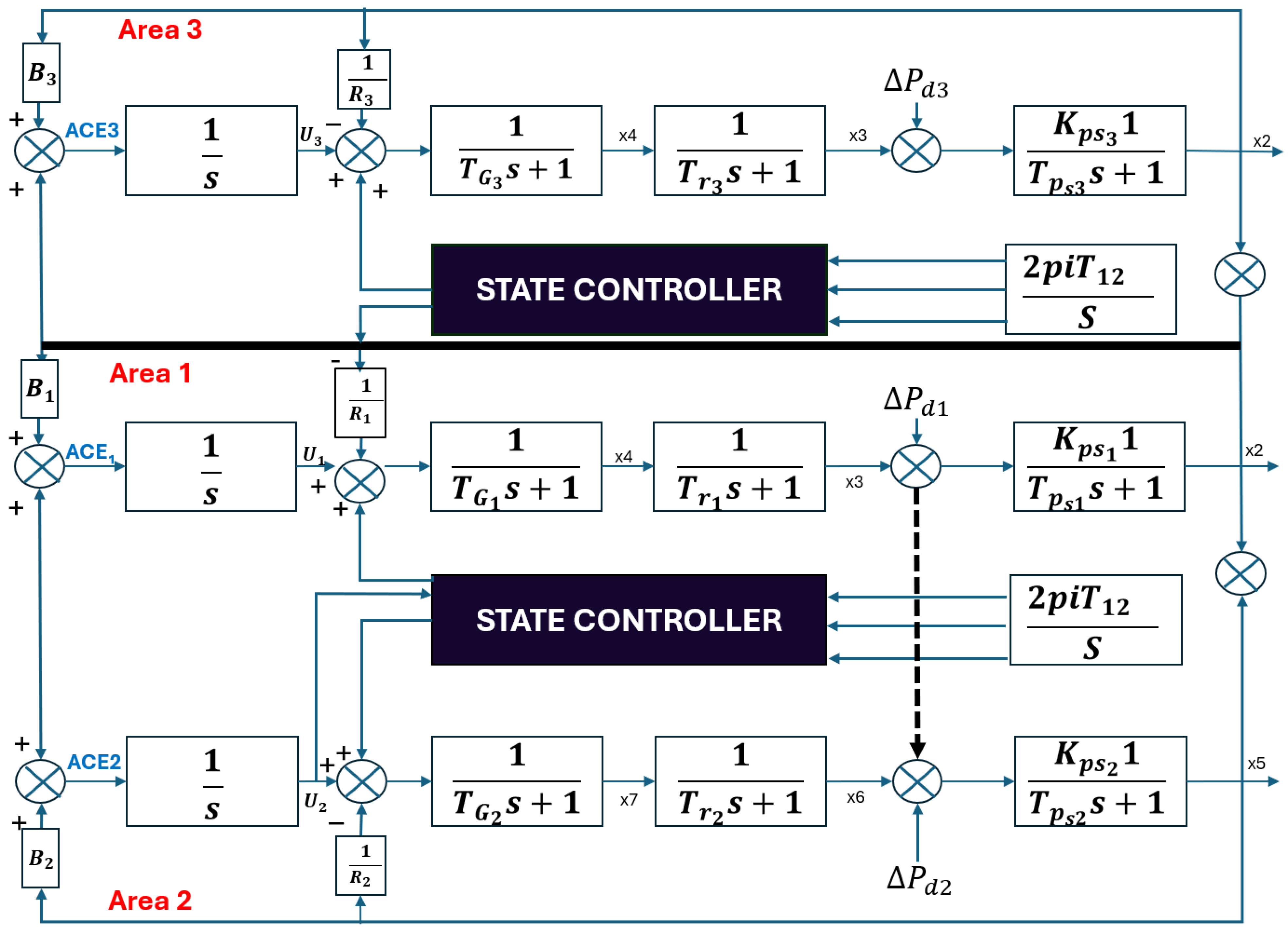
The system comprises three interconnected control areas with nonreheat thermal units. A three-area network is formulated as a discrete-time, centralized, optimal closed-loop structure (Figure 1). To eliminate steady-state frequency errors, the area control errors (ACEs) are included explicitly; their integrals (IACEs) support secondary control. The overall dynamics are expressed in state space [39]. We adopt the sign convention $\mathrm{\Delta }{P}_{ij}>0$ for power flowing from area i to area j. The tie-line exchanges are

$$\begin{array}{cc}\hfill \mathrm{\Delta }{P}_{12}\left(s\right)& ={\displaystyle \frac{2\pi P_{s12}}{s}}\left(\mathrm{\Delta }{f}_1\left(s\right)-\mathrm{\Delta }{f}_2\left(s\right)\right),\hfill \end{array}$$

(1)

$$\begin{array}{cc}\hfill \mathrm{\Delta }{P}_{13}\left(s\right)& ={\displaystyle \frac{2\pi P_{s13}}{s}}\left(\mathrm{\Delta }{f}_1\left(s\right)-\mathrm{\Delta }{f}_3\left(s\right)\right).\hfill \end{array}$$

(2)

In the time domain:

$$\begin{array}{cc}\hfill {\dot{\mathrm{\Delta }P}}_{12}\left(t\right)& =2\pi P_{s12}\left(\mathrm{\Delta }{f}_1\left(t\right)-\mathrm{\Delta }{f}_2\left(t\right)\right),\hfill \end{array}$$

(3)

$$\begin{array}{cc}\hfill {\dot{\mathrm{\Delta }P}}_{13}\left(t\right)& =2\pi P_{s13}\left(\mathrm{\Delta }{f}_1\left(t\right)-\mathrm{\Delta }{f}_3\left(t\right)\right).\hfill \end{array}$$

(4)

The ACEs are

$$\begin{array}{cc}\hfill AC{E}_1& ={\beta }_1\mathrm{\Delta }{f}_1+\mathrm{\Delta }{P}_{12}+\mathrm{\Delta }{P}_{13},\hfill \end{array}$$

(5)

$$\begin{array}{cc}\hfill AC{E}_2& ={\beta }_2\mathrm{\Delta }{f}_2-\mathrm{\Delta }{P}_{12},\hfill \end{array}$$

(6)

$$\begin{array}{cc}\hfill AC{E}_3& ={\beta }_3\mathrm{\Delta }{f}_3-\mathrm{\Delta }{P}_{13}.\hfill \end{array}$$

(7)

Area 1 dynamics:

$$\begin{array}{cc}\hfill {\dot{\mathrm{\Delta }f}}_1& ={\displaystyle \frac{K_{ps1}}{T_{ps1}}}\left(\mathrm{\Delta }{P}_{m1}-\mathrm{\Delta }{P}_{L1}-\mathrm{\Delta }{P}_{12}-\mathrm{\Delta }{P}_{13}\right)-{\displaystyle \frac{1}{T_{ps1}}}\mathrm{\Delta }{f}_1,\hfill \\ \hfill {\dot{\mathrm{\Delta }P}}_{m1}& =-{\displaystyle \frac{1}{T_{T1}}}\mathrm{\Delta }{P}_{m1}+{\displaystyle \frac{1}{T_{T1}}}\mathrm{\Delta }{P}_{v1},\hfill \\ \hfill {\dot{\mathrm{\Delta }P}}_{v1}& =-{\displaystyle \frac{1}{T_{G1}{R}_1}}\mathrm{\Delta }{f}_1-{\displaystyle \frac{1}{T_{G1}}}\mathrm{\Delta }{P}_{v1}+{\displaystyle \frac{1}{T_{G1}}}{u}_1.\hfill \end{array}$$

(8)

Area 2 dynamics (with $\mathrm{\Delta }{P}_{12}>0$ an inflow):

$$\begin{array}{cc}\hfill {\dot{\mathrm{\Delta }f}}_2& ={\displaystyle \frac{K_{ps2}}{T_{ps2}}}\left(\mathrm{\Delta }{P}_{m2}-\mathrm{\Delta }{P}_{L2}\right)-{\displaystyle \frac{1}{T_{ps2}}}\mathrm{\Delta }{f}_2+{\displaystyle \frac{K_{ps2}}{T_{ps2}}}\mathrm{\Delta }{P}_{12},\hfill \\ \hfill {\dot{\mathrm{\Delta }P}}_{m2}& =-{\displaystyle \frac{1}{T_{T2}}}\mathrm{\Delta }{P}_{m2}+{\displaystyle \frac{1}{T_{T2}}}\mathrm{\Delta }{P}_{v2},\hfill \\ \hfill {\dot{\mathrm{\Delta }P}}_{v2}& =-{\displaystyle \frac{1}{T_{G2}{R}_2}}\mathrm{\Delta }{f}_2-{\displaystyle \frac{1}{T_{G2}}}\mathrm{\Delta }{P}_{v2}+{\displaystyle \frac{1}{T_{G2}}}{u}_2.\hfill \end{array}$$

(9)

Area 3 dynamics (with $\mathrm{\Delta }{P}_{13}>0$ an inflow):

$$\begin{array}{cc}\hfill {\dot{\mathrm{\Delta }f}}_3& ={\displaystyle \frac{K_{ps3}}{T_{ps3}}}\left(\mathrm{\Delta }{P}_{m3}-\mathrm{\Delta }{P}_{L3}\right)-{\displaystyle \frac{1}{T_{ps3}}}\mathrm{\Delta }{f}_3+{\displaystyle \frac{K_{ps3}}{T_{ps3}}}\mathrm{\Delta }{P}_{13},\hfill \\ \hfill {\dot{\mathrm{\Delta }P}}_{m3}& =-{\displaystyle \frac{1}{T_{T3}}}\mathrm{\Delta }{P}_{m3}+{\displaystyle \frac{1}{T_{T3}}}\mathrm{\Delta }{P}_{v3},\hfill \\ \hfill {\dot{\mathrm{\Delta }P}}_{v3}& =-{\displaystyle \frac{1}{T_{G3}{R}_3}}\mathrm{\Delta }{f}_3-{\displaystyle \frac{1}{T_{G3}}}\mathrm{\Delta }{P}_{v3}+{\displaystyle \frac{1}{T_{G3}}}{u}_3.\hfill \end{array}$$

(10)

$$\begin{array}{cc}\hfill {\displaystyle \frac{dIAC{E}_1\left(t\right)}{dt}}& =AC{E}_1\left(t\right),\hfill \end{array}$$

(11)

$$\begin{array}{cc}\hfill {\displaystyle \frac{dIAC{E}_2\left(t\right)}{dt}}& =AC{E}_2\left(t\right),\hfill \end{array}$$

(12)

$$\begin{array}{cc}\hfill {\displaystyle \frac{dIAC{E}_3\left(t\right)}{dt}}& =AC{E}_3\left(t\right).\hfill \end{array}$$

(13)

$$\begin{array}{cc}\hfill {\mathbf{x}}^{\top }= & [\mathrm{\Delta }{P}_{12},\mathrm{\Delta }{P}_{13},\mathrm{\Delta }{f}_1,\mathrm{\Delta }{P}_{m1},\mathrm{\Delta }{P}_{v1},\mathrm{\Delta }{f}_2,\mathrm{\Delta }{P}_{m2},\mathrm{\Delta }{P}_{v2},\mathrm{\Delta }{f}_3,\mathrm{\Delta }{P}_{m3},\mathrm{\Delta }{P}_{v3},\hfill \\ \hfill & AC{E}_1,AC{E}_2,AC{E}_3,IAC{E}_1,IAC{E}_2,IAC{E}_3].\hfill \end{array}$$

(14)

Each area contains a governor–turbine loop, power–frequency dynamics, and an ACE feedback path. The centralized state controller receives the augmented state vector (frequencies, tie-line deviations, governor, turbine states, and ACE/IACE) from all three areas and returns coordinated control signals $u_1$, $u_2$, and $u_3$. Tie-line interactions between the areas are illustrated by the power flows $\mathrm{\Delta }{P}_{12}$, $\mathrm{\Delta }{P}_{13}$, and $\mathrm{\Delta }{P}_{23}$. The diagram clearly separates the three channels and highlights the structural symmetry of the model.

2.2. Discretization

AGC is implemented on digital SCADA/EMS platforms, where measurements and control signals are updated at discrete sampling instants. Therefore, the controller must be designed in discrete time and the LQR gain is computed from the discrete algebraic Riccati equation rather than a purely continuous-time formulation.

The continuous-time matrices $A_c$, $B_c$, and ${\mathrm{\Gamma }}_c$ are converted to their discrete-time counterparts $A_d$, $B_d$, and ${\mathrm{\Gamma }}_d$ using the one-step forward–Euler discretization [15,39]. The sampling interval is set to $T=0.814$ s, and is chosen to match the sampling interval used in the discrete-time AGC study of Esmail and Krishnamurthy [45], while our model is a three-area nonreheat thermal system and is chosen to balance numerical stability and real-time implementability with respect to the dominant governor–turbine time constants. The relationships used for conversion are

$$\begin{array}{cc}\hfill A_d& =I+T{A}_c,\hfill \end{array}$$

(15)

$$\begin{array}{cc}\hfill B_d& =T{B}_c,\hfill \end{array}$$

(16)

$$\begin{array}{cc}\hfill {\mathrm{\Gamma }}_d& =T{\mathrm{\Gamma }}_c.\hfill \end{array}$$

(17)

where I denotes the identity matrix and T is the sampling period.

2.3. Functional Minimization Method

Considering the performance criteria involving the area control errors (ACEs), their integral counterparts (IACEs), and the control efforts $u_1$, $u_2$, and $u_3$, the discrete-time quadratic cost function is formulated as

$$\begin{array}{cc}\hfill J={\displaystyle \frac{1}{2}}\sum _{k=k_0}^{\infty }& [{\mathrm{ACE}}_1^2+{\mathrm{ACE}}_2^2+{\mathrm{ACE}}_3^2+{\mathrm{IACE}}_1^2+{\mathrm{IACE}}_2^2\hfill \\ \hfill & +{\mathrm{IACE}}_3^2+u_1^2+u_2^2+u_3^2]\hfill \end{array}$$

(18)

Expanding the ACE terms using the definitions in the system model gives:

$$\begin{array}{cc}\hfill J={\displaystyle \frac{1}{2}}\sum _{k=k_0}^{\infty }& [{({\beta }_1\mathrm{\Delta }{f}_1+\mathrm{\Delta }{P}_{12}+\mathrm{\Delta }{P}_{13})}^2+{({\beta }_2\mathrm{\Delta }{f}_2-\mathrm{\Delta }{P}_{12})}^2\hfill \\ \hfill & +{({\beta }_3\mathrm{\Delta }{f}_3-\mathrm{\Delta }{P}_{13})}^2+{\mathrm{IACE}}_1^2+{\mathrm{IACE}}_2^2\hfill \\ \hfill & +{\mathrm{IACE}}_3^2+u_1^2+u_2^2+u_3^2]\hfill \end{array}$$

(19)

2.4. LQR Controller Design

The discrete-time system dynamics are defined as follows:

$$x(k+1)=A_{d}x\left(k\right)+B_{d}u\left(k\right)+{\mathrm{\Gamma }}_{d}w\left(k\right)$$

(20)

where $x\left(k\right)$ is the state vector, $u\left(k\right)$ is the control input, and $w\left(k\right)$ is the disturbance. The cost function to be minimized is

$$J={\displaystyle \frac{1}{2}}\sum _{k=k_0}^{\infty }(x^{\top }\left(k\right)Q_{d}x\left(k\right)+u^{\top }\left(k\right)R_{d}u\left(k\right))$$

(21)

where $Q_d$ and $R_d$ are symmetric positive-definite weighting matrices that penalize deviations in states and control effort, respectively.

The disturbance term ${\mathrm{\Gamma }}_{d}w\left(k\right)$ is additive and does not affect the optimal feedback gain due to the certainty equivalence principle. The optimal control law is derived using dynamic programming and the Bellman equation. Assume the value function (minimum cost-to-go) is quadratic:

$$V(k,x\left(k\right))={\displaystyle \frac{1}{2}}f{x}^{\top }\left(k\right)Px\left(k\right)$$

(22)

where P is a symmetric positive-definite matrix. Applying the Bellman equation:

$$\begin{gathered} V(k,x\left(k\right))=\underset{u\left(k\right)}{min}\left[{\displaystyle \frac{1}{2}}\left(x^{\top }{Q}_{d}x+u^{\top }{R}_{d}u\right) \\ +V(k+1,x(k+1\left)\right)\right] \end{gathered}$$

(23)

Substituting $x(k+1)=A_{d}x\left(k\right)+B_{d}u\left(k\right)+{\mathrm{\Gamma }}_{d}w\left(k\right)$ into the value function:

$$\begin{gathered} V(k,x\left(k\right))=\underset{u\left(k\right)}{min}[{\displaystyle \frac{1}{2}}\left(x^{\top }{Q}_{d}x+u^{\top }{R}_{d}u\right) \\ +{\displaystyle \frac{1}{2}}{\left(A_{d}x+B_{d}u\right)}^{\top }P\left(A_{d}x+B_{d}u\right)] \end{gathered}$$

(24)

Taking the gradient with respect to $u\left(k\right)$ and setting it to zero:

$$(R_d+B_d^{\top }P{B}_d)u+B_d^{\top }P{A}_{d}x=0$$

(25)

Solving for the optimal control input:

$$u\left(k\right)=-{\left(R_d+B_d^{\top }P{B}_d\right)}^{-1}{B}_d^{\top }P{A}_{d}x\left(k\right)$$

(26)

Therefore, the optimal feedback control law is

$$u\left(k\right)=-Kx\left(k\right)$$

(27)

with the feedback gain:

$$K={\left(R_d+B_d^{\top }P{B}_d\right)}^{-1}{B}_d^{\top }P{A}_d$$

(28)

In practice, the FMM translates the design objectives (small ACE/IACE and moderate control effort) into a quadratic cost and uses the resulting sensitivities to construct the weighting matrices $Q_d$ and $R_d$ as summarized in Algorithm 1.

Algorithm 1 FMM-based selection of $Q_d$ and $R_d$.

1: Define a quadratic cost J that penalizes $AC{E}_i$, $IAC{E}_i$, and $u_i$ over a chosen horizon. 2: For each state $x_i$ and control input $u_j$, compute $𝜕J/𝜕x_i$ and $𝜕J/𝜕u_j$ along a representative disturbance (e.g., step load). 3: Set the diagonal elements of $Q_d$ and $R_d$ proportional to the magnitudes of these derivatives and normalize the matrices. 4: Solve the discrete-time LQR with $(Q_d,R_d)$ to obtain K; if the closed-loop ACE/IACE and control profiles do not meet the AGC requirements, adjust the relative weights and repeat Steps 2–4.

2.5. System Flowchart

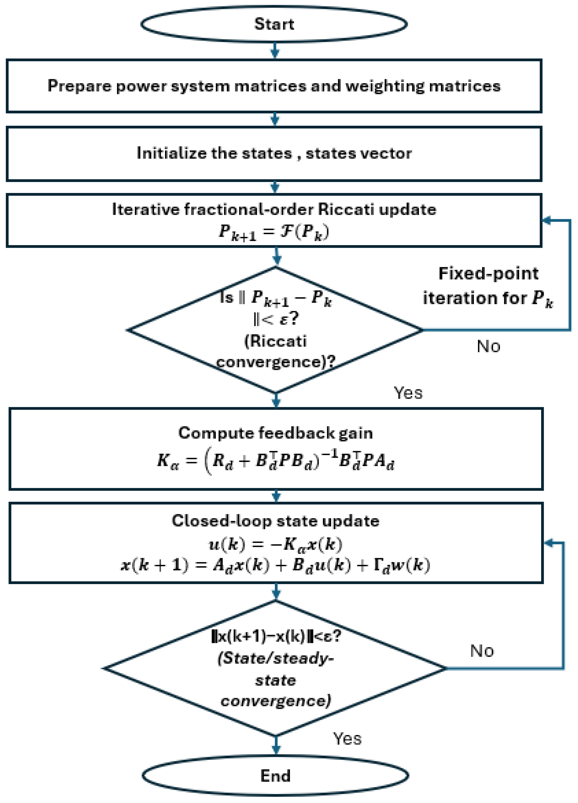
The computational workflow for the proposed centralized AGC design is summarized in Figure 2. The flowchart illustrates the unified procedure used for both the classical discrete-time LQR controller (COQAGC), obtained when $\alpha =1$, and the fractional-order LQR (FOLQR) controller for $0<\alpha <1$. In the fractional case, the Riccati equation is solved iteratively until the sequence $\parallel P_{k+1}-P_k\parallel <\epsilon$ is satisfied, after which the corresponding gain $K_{\alpha }$ is computed and used for closed-loop simulation.

The implementation begins by formulating the interconnected multi-area thermal system in the continuous-time state-space domain, including governor–turbine dynamics, tie-line power flows, and the augmented ACE/IACE states. The model is then discretized using the forward–Euler method with sampling time T, which is consistent with digital AGC operation and with discrete-time AGC formulations in previous studies.

After selecting the weighting matrices $(Q_d,R_d)$ using the functional minimization method, the fractional-order Riccati update is iterated until the matrix sequence $P_k$ converges. Once $K_{\alpha }$ is obtained, the closed-loop system is simulated by repeatedly applying the control law $u\left(k\right)=-K_{\alpha }x\left(k\right)$ and updating the state

$$x(k+1)=A_{d}x\left(k\right)+B_{d}u\left(k\right)+{\mathrm{\Gamma }}_{d}w\left(k\right),$$

until the condition $\parallel x(k+1)-x\left(k\right)\parallel <\epsilon$ (steady-state convergence) is met. The resulting trajectories of frequency deviations, ACE responses, tie-line flows, and control signals are then logged and analyzed for performance evaluation under various step-load disturbances.

In order to make the implementation steps explicit, the proposed FOLQR-based centralized AGC scheme is summarized in Algorithm 2.

Algorithm 2 Proposed FOLQR-based centralized AGC algorithm

1: Input: Continuous-time plant parameters; tie-line data; sampling time T; fractional order $\alpha$; disturbance profiles $w\left(k\right)$. 2: Build continuous-time model: Form the augmented state-space model $(A_c,B_c,{\mathrm{\Gamma }}_c)$ including frequency, governor–turbine, tie-line, and  ACE/IACE dynamics. 3: Discretize system: Apply the forward–Euler method with sampling time T to obtain the discrete-time matrices $(A_d,B_d,{\mathrm{\Gamma }}_d)$. 4: Select weighting matrices via FMM: Define a quadratic cost that penalizes $AC{E}_i$, $IAC{E}_i$, and $u_i$. Evaluate the sensitivities $𝜕J/𝜕x_i$ and $𝜕J/𝜕u_j$ along a representative disturbance. Set and normalize the diagonal entries of $Q_d$ and $R_d$ proportionally to these sensitivities. 5: Compute FOLQR gain: Solve the fractional-order Riccati equation (for the chosen $\alpha$ and $(Q_d,R_d)$) iteratively until $\parallel P_{k+1}-P_k\parallel <\epsilon$ is satisfied, and obtain the steady-state solution $P_{\alpha }$ and the corresponding feedback gain $$K_{\alpha }={(R_d+B_d^{\top }{P}_{\alpha }{B}_d)}^{-1}{B}_d^{\top }{P}_{\alpha }{A}_d.$$ (For $\alpha =1$, this reduces to the conventional discrete-time LQR gain.) 6: Closed-loop simulation: 1. For each disturbance case, initialize the state vector $x\left(0\right)$. 2. For $k=0,1,\dots$: (a) Compute the control input $u\left(k\right)=-K_{\alpha }x\left(k\right)$ (including GRC/saturation if modeled). (b) Update the state $x(k+1)=A_{d}x\left(k\right)+B_{d}u\left(k\right)+{\mathrm{\Gamma }}_{d}w\left(k\right)$. (c) Log $\mathrm{\Delta }{f}_i\left(k\right)$, $AC{E}_i\left(k\right)$, $\mathrm{\Delta }{P}_{ij}\left(k\right)$, and $u_i\left(k\right)$. 3. Stop when the specified simulation horizon is reached or a settling criterion on $x\left(k\right)$ is met. 7: Performance evaluation: From the logged trajectories, compute peak deviations, settling times, and other performance metrics; compare FOLQR against the COQAGC (LQR) baseline and existing AGC controllers from the literature.

2.6. Fractional–Order Dynamics and Their Role in the Proposed FOLQR Scheme

In this subsection, we recall the notion of a fractional–order LTI system and clarify how it is used in the proposed fractional–order LQR (FOLQR)-based AGC design.

2.6.1. Physical Plant (Integer–Order Model)

The three-area AGC plant is modeled by the classical integer-order differential equations in (8)–(10). These equations describe the frequency, turbine, governor, tie-line and integral-error dynamics using first-order time derivatives, i.e.,

$$\dot{x}\left(t\right)=Ax\left(t\right)+Bu\left(t\right)+\mathrm{\Gamma }\mathrm{\Delta }{P}_L\left(t\right),$$

(29)

where $x\left(t\right)\in {\mathbb{R}}^n$ collects all state variables, $u\left(t\right)\in {\mathbb{R}}^m$ is the vector of control inputs, $\mathrm{\Delta }{P}_L\left(t\right)$ denotes the load disturbances, and A, B, $\mathrm{\Gamma }$ are constant matrices obtained from the classical AGC model. Equation (29) is the only equation that represents the physics of the interconnected power system.

2.6.2. Fractional–Order LTI Template

For the FOLQR controller, we employ the standard Caputo fractional-order LTI model of order $\alpha \in (0,1]$:

$${{}^{C}D}_t^{\alpha }x\left(t\right)=Ax\left(t\right)+Bu\left(t\right),x\left(0\right)=x_0,$$

(30)

where ${{}^{C}D}_t^{\alpha }$ denotes the Caputo fractional derivative of order $\alpha$ and $A,B$ are constant matrices. Equation (30) is not introduced as a new physical model of the AGC plant. Instead, it serves as a mathematical template to describe the closed–loop dynamics when a fractional–order LQR state–feedback law is applied.

The fundamental solution of (30) is expressed in terms of the matrix Mittag–Leffler function

$$E_{\alpha ,\beta }\left(A{t}^{\alpha }\right)\triangleq \sum _{k=0}^{\infty }{\displaystyle \frac{{\left(A{t}^{\alpha }\right)}^k}{\mathrm{\Gamma }(\alpha k+\beta )}},E_{\alpha }\left(A{t}^{\alpha }\right)\equiv E_{\alpha ,1}\left(A{t}^{\alpha }\right),$$

(31)

and the corresponding state response is

$$x\left(t\right)=E_{\alpha }\left(A{t}^{\alpha }\right)x_0+{\int }_0^t{(t-\tau )}^{\alpha -1}{E}_{\alpha ,\alpha }\left(A{(t-\tau )}^{\alpha }\right)Bu\left(\tau \right)d\tau .$$

(32)

2.6.3. Application to the AGC Closed–Loop System

Starting from the integer-order plant (29), the LQR and FOLQR controllers use state feedback of the form

$$u\left(t\right)=-Kx\left(t\right),u_{\alpha }\left(t\right)=-K_{\alpha }x\left(t\right),$$

(33)

where K is the classical LQR gain (for $\alpha =1$) and $K_{\alpha }$ is the gain obtained from the FOLQR design with weighting matrices $Q_F$ and $R_F$.

Substituting $u_{\alpha }\left(t\right)$ into (29) yields the integer-order closed-loop dynamics

$$\dot{x}\left(t\right)=(A-B{K}_{\alpha })x\left(t\right)+\mathrm{\Gamma }\mathrm{\Delta }{P}_L\left(t\right).$$

(34)

To introduce fractional-order behavior at the control design level, we reinterpret the closed-loop derivative in the Caputo sense and model the trajectories under FOLQR as

$${{}^{C}D}_t^{\alpha }x\left(t\right)=(A-B{K}_{\alpha })x\left(t\right)+\mathrm{\Gamma }\mathrm{\Delta }{P}_L\left(t\right),0<\alpha \le 1.$$

(35)

Comparing (35) with the template (30), we observe that the same matrices A, B, and $\mathrm{\Gamma }$ derived from the classical AGC model are used; only the order of the derivative is generalized from 1 to $\alpha$. Therefore, the fractional operator acts solely at the level of the closed–loop state dynamics and does not alter the underlying physical plant Equations (8)–(10).

For $\alpha =1$, (35) reduces to the classical integer–order closed–loop system driven by the LQR gain. For $0<\alpha <1$, the Caputo derivative introduces memory (hereditary) effects that modify the transient response. In the simulations, (35) is integrated numerically using a predictor–corrector scheme for Caputo fractional differential equations, with the same initial conditions and disturbance profiles as in the LQR case. This ensures a fair comparison between LQR and FOLQR on the same underlying AGC plant.

2.7. Fundamental Solution and State Response

Using the Laplace transform identity

$$\mathcal{L}\left\{t^{\beta -1}{E}_{\alpha ,\beta }\left(A{t}^{\alpha }\right)\right\}=s^{\alpha -\beta }{\left(s^{\alpha }I-A\right)}^{-1},$$

(36)

the unique solution of (32) is

$$\begin{array}{cc}\hfill x\left(t\right)=& E_{\alpha }\left(A{t}^{\alpha }\right)x_0\hfill \\ \hfill & +{\int }_0^t{(t-\tau )}^{\alpha -1}{E}_{\alpha ,\alpha }\left(A{(t-\tau )}^{\alpha }\right)Bu\left(\tau \right)\mathrm{d}\tau .\hfill \end{array}$$

(37)

Equation (37) generalizes the classical matrix-exponential response to the fractional-order setting.

3. Results and Discussion

Performance metrics: Overshoot is reported as the peak deviation relative to the pre-disturbance value (undershoot shown as negative), and settling time is the time taken to enter and remain within a ±2% band of the final value.

3.1. Case 1: Dynamic Response to a Small Step-Load Disturbance

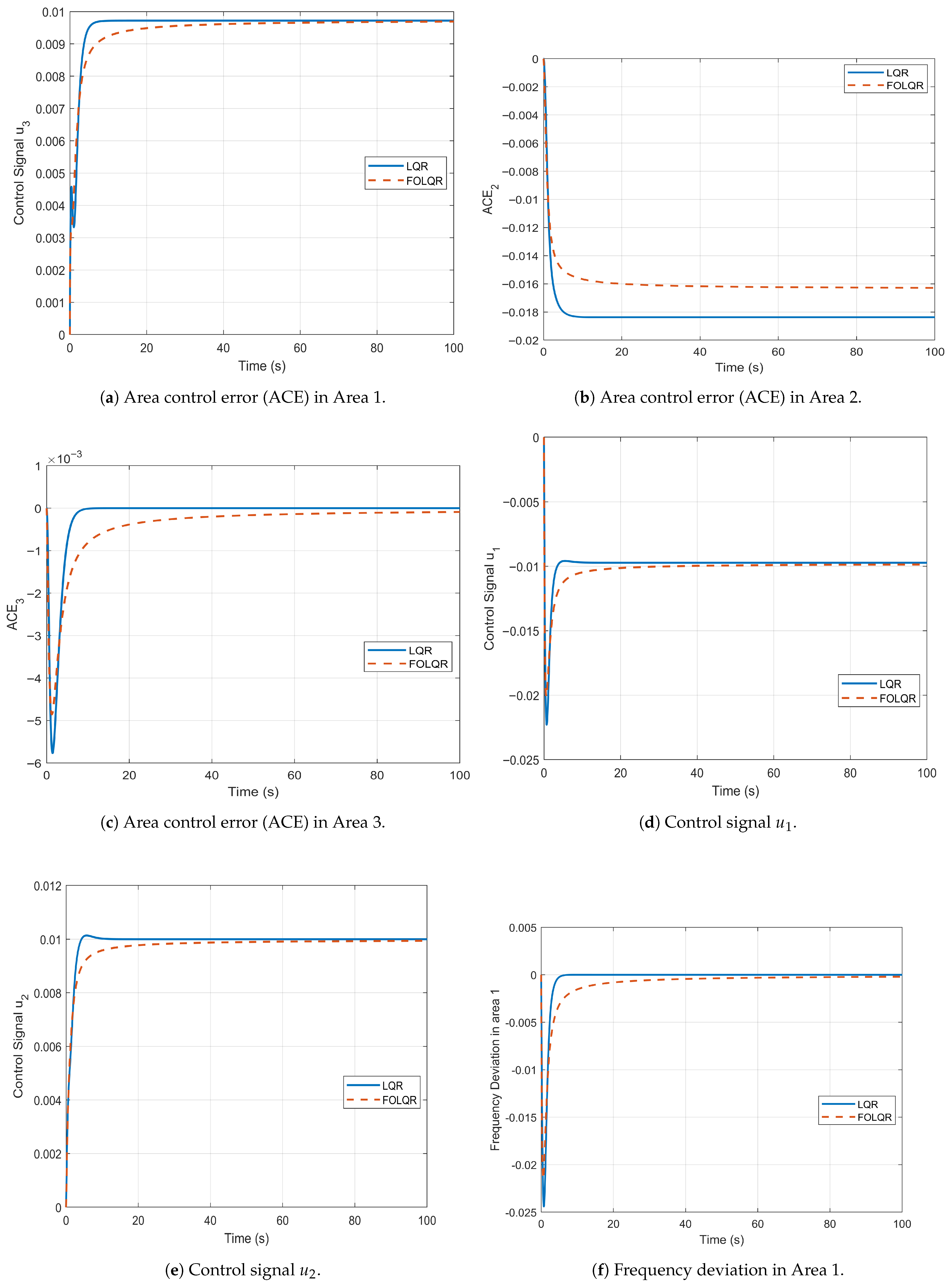
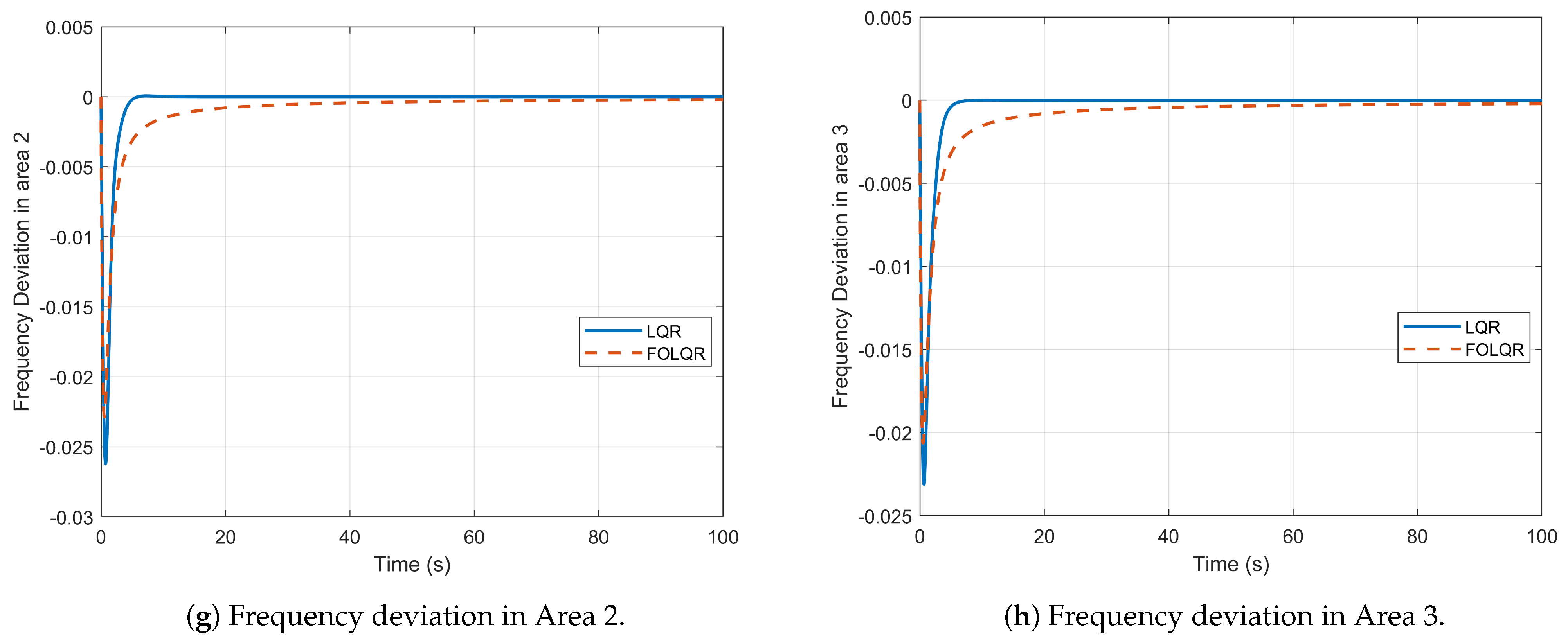
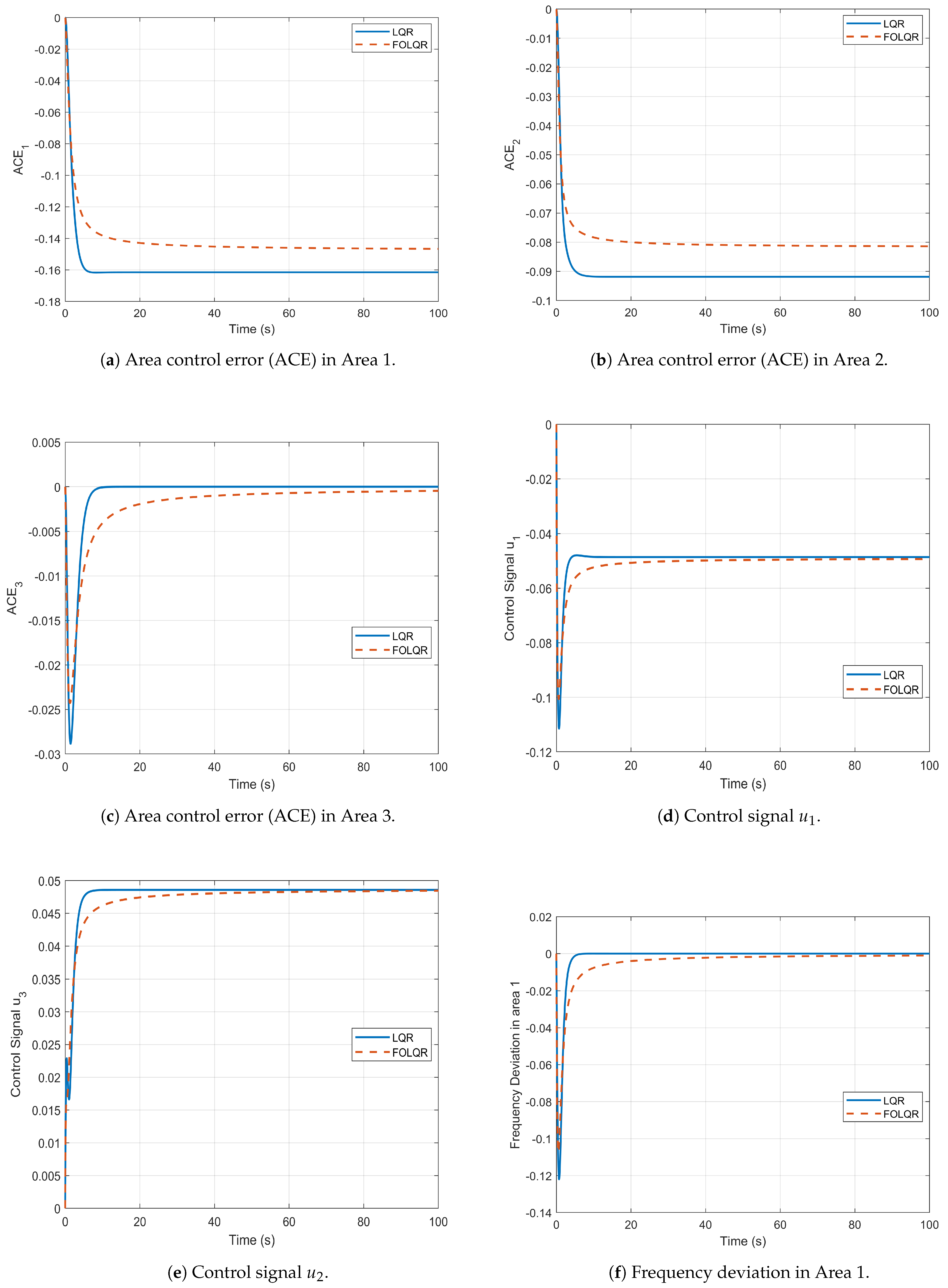
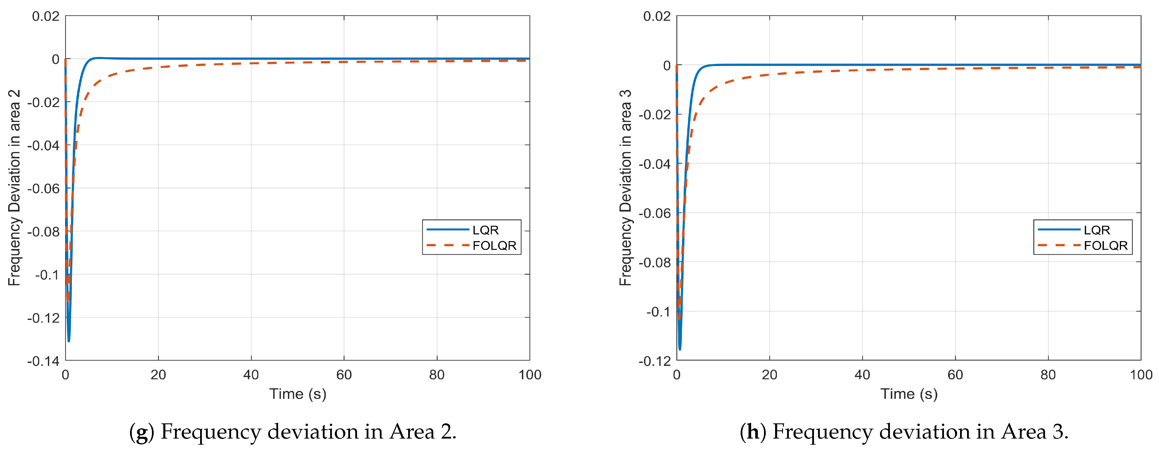
Case 1 evaluates the system’s dynamic behavior in response to a 0.01 p.u. step-load disturbance applied at $t=0$ s. Frequency deviations. Following a 0.01 pu load step, As illustrated in Figure 3f–h all three areas exhibit an initial undershoot on the order of ${10}^{-2}$ puHz. The LQR responses dip slightly deeper during the first couple of seconds, reflecting a more aggressive early correction, and they return to nominal more rapidly (within single-digit seconds) than the FOLQR trajectories. The FOLLQR responses display a smoother, more gradual exponential-like recovery. Over the simulation horizon, both controllers restore the frequencies to practically zero, with the essential distinction being LQR’s faster clean-up versus FOLQR’s gentler transient.

Area control error (ACE): Both controllers substantially attenuate $AC{E}_i$ in all areas. As shown in Figure 3a–c, ACE settles to small constant negative values within the simulated window, with LQR reaching its asymptote more quickly than FOLQR. In Area 3, $ACE$ decays the fastest and ends closest to zero under LQR, while FO-LQR approaches the neighborhood of zero more gradually.

Control effort: As shown in Figure 3d,e the synthesized control signals $u_1$ and $u_2$ reveal a clear transient-effort trade-off. LQR produces larger peak magnitudes and faster changes by inspection, roughly 5–15% higher peaks across the three inputs whereas FOLQR yields smoother commands with smaller extrema and a slower approach to the steady value. Both methods converge to very similar steady control levels, implying comparable steady state allocation; the principal difference lies in how aggressively each controller responds during the transient.

System-level behavior: The disturbance propagates coherently across the interconnection: all areas exhibit qualitatively similar frequency and ACE dynamics, confirming appropriate tie-line coupling and coordinated secondary control. LQR’s faster decay of $\mathrm{\Delta }{f}_i$ aligns with its more forceful transient inputs, whereas the fractional dynamics in FOLQR act like a memory term that tempers rapid changes and prioritizes smoothness. The residual $ACE$ in Areas 1 and 2 within the simulated window suggests that tie-line power deviations are sharing part of the regulation burden; integral augmentation or weight retuning would help drive $ACE$ closer to zero without sacrificing inter-area coordination.

3.2. Case 2: Dynamic Response to a Larger Step-Load Disturbance

Case 2 evaluates the system response to a larger step-load disturbance of 0.05 p.u. applied at $t=0$ s.

Frequency deviations. With a larger 0.05 pu load step, the frequency trajectories shown in (Figure 4f–h) preserve the qualitative behavior observed in Case 1 while scaling in magnitude by roughly a factor of five. LQR exhibits a deeper initial undershoot (about $-0.12$ to $-0.13$ puHz) compared with FOLQR, consistent with its more aggressive early correction. Nevertheless, LQR restores the frequency to nominal noticeably faster—within a few seconds—whereas FOLQR follows a smoother, more gradual recovery with a longer tail. Over the simulated window, both controllers bring the frequency deviation close to zero, with the main distinction remaining the classic speed–smoothness trade-off.

Area control error (ACE): Both designs suppress $ACE$ rapidly across the three areas. In Areas 1 and 2, $ACE$ settles to small constant negative values within the horizon, as shown in Figure 4a–c with LQR reaching its asymptote more quickly than FOLQR as in Figure 3c. In Area 3, $AC{E}_3$ decays the fastest and approaches the vicinity of zero, again with LQR leading in convergence speed and FOLQR approaching more gradually.

Control effort: The control inputs as shown in Figure 4d,e $u_1$, $u_2$, and $u_3$ remain well-behaved under the larger disturbance and scale approximately linearly with the step size (peak values about five times those in Case 1). LQR produces larger transient peaks and faster changes by visual inspection, a few percent higher than FOLQR before settling to nearly identical steady values. FOLQR yields smoother commands with smaller extrema and a slower approach to steady state, reflecting the damping effect of the fractional dynamics on high-frequency control action.

System-level behavior: The disturbance propagates coherently across the interconnection, with the areas exhibiting similar qualitative dynamics in frequency, $ACE$, and control effort. LQR’s faster decay in $\mathrm{\Delta }f$ aligns with its more forceful early actuation, while the FOLQR controller prioritizes smoother transients at the expense of longer recovery. No evidence of actuator saturation is apparent in the plotted inputs for the 0.05 pu step, suggesting adequate control headroom for both designs under this operating condition.

Overall assessment for Case 2: Under a fivefold increase in disturbance magnitude, both controllers preserve stability and deliver acceptable secondary control performance. LQR remains preferable when rapid frequency restoration is paramount, whereas FOLQR offers a compelling alternative when smoother actuation and reduced peak control effort are prioritized. The addition of integral action on $ACE$ (LQI/FOLQI) or modest retuning would further tighten $ACE$ regulation in all areas.

Overall comparison: Across both disturbance levels (0.01 and 0.05 pu), the relative ordering of the two designs is consistent: LQR achieves faster frequency clean-up and reaches the $ACE$ asymptotes sooner, while FOLQR delivers smoother transients with slightly smaller control peaks. Responses scale nearly linearly with the step size in terms of frequency undershoot and control-input magnitudes, which is expected for the linearized plant and quadratic-feedback structure.

Table 1. Overshoot comparison for different controllers (all values in Hz for $\mathrm{\Delta }{f}_i$ and p.u. for $\mathrm{\Delta }{P}_{ij}$).

Controller (Source)	$\mathbf{\Delta }{\mathit{f}}_1$ (Hz)	$\mathbf{\Delta }{\mathit{f}}_2$ (Hz)	$\mathbf{\Delta }{\mathit{f}}_3$ (Hz)	$\mathbf{\Delta }{\mathit{P}}_{12}$ (p.u.)	$\mathbf{\Delta }{\mathit{P}}_{13}$ (p.u.)
TLBO-PIDD [44]	$1.30\times {10}^{-1}$	$1.50\times {10}^{-1}$	–	$-3.70\times {10}^{-2}$	–
GCOQAGCC [45]	$-1.30\times {10}^{-1}$	$1.50\times {10}^{-1}$	–	$-1.70\times {10}^{-2}$	–
COQAGC [45]	$2.44\times {10}^{-2}$	$2.62\times {10}^{-2}$	–	$6.60\times {10}^{-4}$	–
FOLQR	$2.15\times {10}^{-2}$	$2.30\times {10}^{-2}$	$2.10\times {10}^{-2}$	$5.00\times {10}^{-4}$	$5.50\times {10}^{-4}$

and

Table 2. Settling time comparison for different controllers.

Controller	$\mathbf{\Delta }{\mathit{f}}_1$ (Hz)	$\mathbf{\Delta }{\mathit{f}}_2$ (Hz)	$\mathbf{\Delta }{\mathit{f}}_3$ (Hz)	$\mathbf{\Delta }{\mathit{P}}_{12}$ (p.u.)	$\mathbf{\Delta }{\mathit{P}}_{13}$ (p.u.)
TLBO-PIDD [44]	6.8	3.9	–	6.5	–
GCOQAGCC [45]	4	8	–	8	–
COQAGC [45]	4.3	4.3	–	10.8	–
FOLQR	10	7	11	22	18

summarize overshoot and settling-time performance under a 0.01 p.u. disturbance. From Table 1, the largest frequency-overshoot magnitudes occur for TLBO-PIDD and GCOQAGCC (on the order of ${10}^{-1}$), whereas FGSC and the COQAGC/FOLQR entries are an order of magnitude smaller (on the order of ${10}^{-2}$). For tie-line deviations, FGSC and FOLQR report the smallest magnitudes (from $5.00\times {10}^{-4}$ to $4.00\times {10}^{-4}$), while TLBO-PIDD and GCOQAGCC exhibit larger excursions, including undershoot (negative values). Table 2 lists the corresponding settling times. Across the reported entries, FGSC and GCOQAGCC are in the 4–8 s range, COQAGC spans $4.3$–12 s, and FOLQR spans 7–22 s.

Table 3. Peak deviations for Case 1 (0.01 p.u.) and Case 2 (0.05 p.u.).

Case	Controller	$\mathbf{\Delta }{\mathit{f}}_1$ (Hz)	$\mathbf{\Delta }{\mathit{f}}_2$ (Hz)	$\mathbf{\Delta }{\mathit{f}}_3$ (Hz)	$\mathbf{\Delta }{\mathit{P}}_{12}$ (p.u.)	$\mathbf{\Delta }{\mathit{P}}_{13}$ (p.u.)
Case 1 (0.01 p.u.)	COQAGC	$2.44\times {10}^{-2}$	$2.62\times {10}^{-2}$	$2.31\times {10}^{-2}$	$6.16\times {10}^{-4}$	$1.38\times {10}^{-3}$
Case 1 (0.01 p.u.)	FOLQR	$2.15\times {10}^{-2}$	$2.29\times {10}^{-2}$	$2.06\times {10}^{-2}$	$5.00\times {10}^{-4}$	$5.53\times {10}^{-4}$
Case 2 (0.05 p.u.)	COQAGC	$1.22\times {10}^{-1}$	$1.31\times {10}^{-1}$	$1.16\times {10}^{-1}$	$3.08\times {10}^{-3}$	$6.88\times {10}^{-3}$
Case 2 (0.05 p.u.)	FOLQR	$1.07\times {10}^{-1}$	$1.14\times {10}^{-1}$	$1.03\times {10}^{-1}$	$2.50\times {10}^{-3}$	$2.76\times {10}^{-3}$

contrasts Case 1 (0.01 p.u.) and Case 2 (0.05 p.u.). As expected, both controllers exhibit larger frequency deviations and tie-line excursions in Case 2 than in Case 1 for all listed variables.

4. Conclusions and Future Work

This work proposed and evaluated a discrete-time centralized fractional-order LQR (FOLQR) for automatic generation control of a three-area nonreheat thermal system, together with a systematic comparison against a discrete-time LQR/COQAGC baseline drawn from the literature. Two disturbance levels were studied (0.01 and 0.05 p.u. steps). Across all experiments and in all areas, FOLQR stabilized the interconnection and preserved coherent inter-area coordination while delivering markedly lower peak excursions in both frequency and tie-line power. Relative to COQAGC, FO-LQR reduced peak frequency deviations by roughly 9–$12\%$ and tie-line peaks by 24–$60\%$ in Case 1 and maintained the same low-overshoot character under the larger 0.05 p.u. step. These benefits were accompanied by longer settling times, which is consistent with the smoother actuation produced by the fractional-order dynamics.

For multi-area AGC, where operational limits prioritize constraining overshoot in frequency and tie-line exchanges to avoid protection triggers, contract violations, and actuator stress, the observed trade-off is favorable: FOLQR offers a safer transient profile with smaller peaks and smoother control commands, while still restoring frequencies within practical horizons. The results also show near-linear scaling of key metrics with disturbance size and no evidence of actuator saturation within the tested range, supporting the deployability of FO-LQR under typical operating disturbances. While the present design substantially attenuates the area control error (ACE), the responses suggest that explicitly enforcing $AC{E}_i\to 0$ would benefit from integral augmentation. As such, a promising direction is an FO-LQI variant (or modest retuning of frequency-bias and tie-line weights) to tighten steady ACE regulation without relinquishing FOLQR’s advantage in peak suppression.

Future work will extend the three-area framework to nonlinear plant models, parameter uncertainties, communication delays, actuator constraints and saturations, and larger disturbance scenarios, and will validate the controller through hardware in-the loop and field-facing evaluations in realistic power-system environments. In addition, the proposed FOLQR/COQAGC scheme will be enhanced with attack-resilient and fault-tolerant mechanisms to address cyber threats such as false data injection attacks.

Future work will also investigate event-triggered implementations of the proposed FOLQR-based AGC using adaptive event-triggered output feedback strategies to reduce communication and computational burden while maintaining stability and satisfactory dynamic performance. Moreover, the proposed FOLQR design will be extended to include explicit robustness studies under parameter uncertainties, communication delays, and generation rate constraints in order to more thoroughly assess its practical viability in real interconnected power systems.

References

1. Mohamed, K.A.; Alyazidi, N.M.; Eltayeb, A.; Elferik, S.; Gaufan, K.S.B. Enhancing Load Frequency Control in Single-Area Power Systems: A Comparative Study of PID, FOPID, GA, and PSO-Based Optimization Techniques. In Proceedings of the 2025 IEEE 22nd International Multi-Conference on Systems, Signals & Devices (SSD), Monastir, Tunisia, 17–20 February 2025; pp. 988–993. [Google Scholar] [CrossRef]
2. Mohamed, A.; Mohamed, K.A.; Shafiullah, M.; Saif, A.-W.A. Enhanced Load Frequency Control for Standalone Multi-Source Power Systems Using GWO and GA Optimized. In Proceedings of the 2025 IEEE 22nd International Multi-Conference on Systems, Signals & Devices (SSD), Monastir, Tunisia, 17–20 February 2025; pp. 928–933. [Google Scholar] [CrossRef]
3. Tungadio, D.H.; Bansal, R.C.; Siti, W.W. Optimal control of active power of two micro-grids interconnected with two AC tie-lines. Electr. Power Compon. Syst. 2017, 45, 2188–2199. [Google Scholar] [CrossRef]
4. Delavasi, A.; Afif, S.; Mokriani, L. Load frequency control problem in interconnected power systems: A review. Prot. Control Mod. Power Syst. 2019, 4, 1–25. [Google Scholar]
5. Tan, W.; Xu, Y. Robust analysis and design of load frequency controller for power systems. Electr. Power Syst. Res. 2008, 78, 846–853. [Google Scholar] [CrossRef]
6. Esmail, M.; Tooeirei, R.; Krishnamurthy, S. Review of automatic generation control techniques in interconnected. IFAC-PapersOnLine 2017, 50, 303–308. [Google Scholar] [CrossRef]
7. Khuntia, S.R.; Panda, S. Simulation study for automatic generation control of a multi-area power system using intelligent agents. Appl. Soft Comput. 2012, 12, 133–141. [Google Scholar] [CrossRef]
8. Jangde, R.R.; Sinha, S.K. Simulated tabu neuro-fuzzy hybrid intelligent approach in AGC of a multi-source interconnected power system. Appl. Soft Comput. 2014, 23, 152–164. [Google Scholar]
9. Chan, W.; Men, S.; Ha, Y. Automatic generation control of interconnected power systems using variable-structure controllers. IEEE Proc. D Control Theory Appl. 1991, 138, 579–585. [Google Scholar] [CrossRef]
10. Dong, L.; Zhang, Y.; Gao, Z. A robust decentralized load frequency controller for interconnected power systems. ISA Trans. 2012, 51, 410–419. [Google Scholar] [CrossRef]
11. Wang, Z.Q.; Sznaier, M. Robust control design for load frequency control using H∞ synthesis. In Proceedings of the Conference Record Southcon, Orlando, FL, USA, 29–31 March 1994; p. 198. [Google Scholar]
12. Jalili, A. Optimal PID-based type-2 fuzzy fractional signal control using optimization hybrid power system. Structur. Prop. Solut. 2015, 46, 158–181. [Google Scholar]
13. Fadhil, D.R. Robust and intelligent type-2 fuzzy fractional-order PID-based automatic generation control to eliminate the damping oscillation and mutual interaction between areas. Sustain. Energy Technol. Assess. 2016, 18, 253–259. [Google Scholar]
14. Shang-Guan, X.; He, Z.; Zhang, C.; Fang, J.; Spencer, M.E. Symplectic model-based direct and load frequency control for power systems with thermal power plants. Renew. Energy 2020, 135, 1045. [Google Scholar]
15. Kron, G. Electric Power Systems Dynamics: Theory and Application; Springer: Cham, Switzerland, 2014. [Google Scholar]
16. Yadavalli, K.; Ravi, P.K.; Patadi, P. Sliding mode load-frequency control for power systems. Electr. Power Syst. Res. 2004, 63, 410–417. [Google Scholar]
17. Elgard, O.; Fosha, C. Optimum megawatt-frequency control of multi-area electric energy systems. IEEE Trans. Power App. Syst. 1970, PAS-89, 556–563. [Google Scholar] [CrossRef]
18. Fosha, C.; Elgard, O. The megawatt-frequency control problem: A new approach via optimal control theory. IEEE Trans. Power App. Syst. 1970, PAS-89, 563–577. [Google Scholar] [CrossRef]
19. Abido, M.A.; Gharave, A.A.; Shama, S.S. Design of a novel ABC vector for load-frequency system. Electr. Power Compon. Syst. 2021, 49, 1201–1218. [Google Scholar]
20. Vahidinia, E.; Lakshimi, S.; Halvins, P. Distributed LQR design for a class of large-scale multi-area power systems. Energies 2019, 12, 2654. [Google Scholar]
21. Arya, Z.; Kumar, N.; Gaur, S.K. Optimal automatic generation control of two-area power systems with hybrid sources using deep reinforcement learning. J. Renew. Sustain. Energy 2017, 9, 065103. [Google Scholar] [CrossRef]
22. Sharma, G.; Naudiyal, N.; Niazi, K.R.; Bansal, R.C. Robust automatic generation control design for a two-area power system interconnected via AC/DC tie-lines using an improved sine-cosine algorithm. Int. J. Electr. Power Energy Syst. 2018, 100, 573–580. [Google Scholar]
23. Sharma, S.C. Optimal design for tie-line secure power generation in restructured areas using vector hybrid control technique. Int. J. Eng. Res. Appl. 2019, 45, 99–114. [Google Scholar]
24. Prakash, A.P.; Gupta, S.; Patadi, K. Design of reduced-parameter fuzzy logic and PID controller for automatic generation control of an interconnected power system. Trans. Anal. Appl. 2021, 3, 159–170. [Google Scholar]
25. Das, K.M.; Singh, M.P. TYPE-2 FO-PID controller for automatic generation control of a two-area power system. Renew. Energy Focus 2018, 16, 5611–5619. [Google Scholar]
26. Beerten, D.H.; Kunnie, F. Optimal automatic generation control of large-scale power systems using real-time data and machine learning. Electr. Power Compon. Syst. 2018, 46, 452–462. [Google Scholar]
27. Lalngaihawma, S.; Datta, S.; Das, S. Automatic Generation Control with a Recent ZOA Algorithm Optimized TIDN Controller. In Proceedings of the 2024 IEEE 4th International Conference on Sustainable Energy and Future Electric Transportation (SEFET), Hyderabad, India, 31 July–3 August 2024; pp. 1–6. [Google Scholar] [CrossRef]
28. Kumar, R.; Prasad, U. AGC of Multi-Area Multi-Source Hydrothermal Power Systems Incorporating Renewable Energy Source and Parallel AC-HVDC links via Optimal CFPIDF-PI Controller. In Proceedings of the 2024 Asia Pacific Conference on Innovation in Technology (APCIT), Mysore, India, 26–27 July 2024; pp. 1–6. [Google Scholar] [CrossRef]
29. Ashfaq, T.; Mumtaz, S.; Ahmad, S.; Ullah, B.; Albogamy, F.R. Automatic Generation Control in Renewables-Integrated Multi-Area Power Systems: A Comparative Control Analysis. Sustainability 2024, 16, 5735. [Google Scholar] [CrossRef]
30. Ayyappan, B.P.; Parthiban, T.; Barkavi, M. Generation Control of Multi-Area Multi-Source Power System using Fire-Fly Algorithm. Int. J. Innov. Res. Adv. Eng. 2024, 11, 573–580. [Google Scholar] [CrossRef]
31. Kumar, P.P.; Nuvvula, R.S.; Shezan, S.A.; Satyanarayana, V.; SivaSubramanyamReddy, R.; Ahammed, S.R.; Ali, A. Grid Stability Enhancement through Machine Learning-driven Control Strategies in Renewable Energy Integration. In Proceedings of the 2024 12th International Conference on Smart Grid (icSmartGrid), Setubal, Portugal, 27–29 May 2024. [Google Scholar] [CrossRef]
32. Taha, M.Q.; Elhassene, I.C.; Heiba, B. Gray Wolf Algorithm Optimization of Automatic Generation Control for Deregulated Multi-Area Power System. In Proceedings of the 2024 International Congress on Human-Computer Interaction, Optimization and Robotic Applications (HORA), Istanbul, Turkiye, 23–25 May 2024. [Google Scholar] [CrossRef]
33. Wadhwa, J.; Kumar, N. Analysis of Area-Control Error in Automatic Generation Control. In Proceedings of the 2024 11th International Conference on Reliability, Infocom Technologies and Optimization (Trends and Future Directions) (ICRITO), Noida, India, 14–15 March 2024; pp. 1–6. [Google Scholar] [CrossRef]
34. Illias, H.A.; Nurjannah, N.; Mokhlis, H. Optimization of Automatic Generation Control Performance for Power System of Two-Area based on Genetic Algorithm-Particle Swarm Optimization. In Proceedings of the 2024 IEEE 4th International Conference in Power Engineering Applications (ICPEA), Pulau Pinang, Malaysia, 4–5 March 2024; pp. 317–321. [Google Scholar] [CrossRef]
35. Mishra, R.N.; Kumar, N.; Chaturvedi, D.K. Design and analysis of optimal AGC regulator for multi-area power systems with TCPS and energy storage unit in deregulated environment. Optim. Control Appl. Methods 2024, 45, 1456–1502. [Google Scholar] [CrossRef]
36. Sati, M.M.; Kumar, D.; Singh, A.; Raparthi, M.; Alghayadh, F.Y.; Soni, M. Two-Area Power System with Automatic Generation Control Utilizing PID Control, FOPID, Particle Swarm Optimization, and Genetic Algorithms. In Proceedings of the 2024 Fourth International Conference on Advances in Electrical, Computing, Communication and Sustainable Technologies (ICAECT), Bhilai, India, 11–12 January 2024; pp. 1–6. [Google Scholar] [CrossRef]
37. Mohapatra, K.; Mohapatra, S.; Sahu, P.C.; Samal, P. Load frequency control of a three-area power system using hyHS-RS tuned type-2 fuzzy controller under economic dispatch constraints. In Control Applications in Modern Power Systems; Springer: Singapore, 2024; pp. 261–270. [Google Scholar] [CrossRef]
38. Liao, D.; Li, H.; Wang, J.; Zeng, X.; Wang, X. Research on active coordination control mechanism of provincial and local AGC in power system based on deep learning technology. Appl. Math. Nonlinear Sci. 2024, 9. [Google Scholar] [CrossRef]
39. Esmail, M.; Krishnamurthy, V. Discrete Centralized AGC Using LQR-Based Cost Functional Minimization for Multi-Area Interconnected Power Systems. IEEE Access 2024, 12, 20426–20440. [Google Scholar] [CrossRef]
40. Abdo, Q.M.; Ewad, H.; Mohamed, K.A. Optimized PID Controller for Single Area Thermal Power System Based on Time Varying Acceleration Coefficients Particle Swarm Optimization. In Proceedings of the 020 International Conference on Computer, Control, Electrical, and Electronics Engineering (ICCCEEE), Khartoum, Sudan, 26 February–1 March 2021; pp. 1–5. [Google Scholar] [CrossRef]
41. Singh, V.P.; Waghmare, A.V.; Meena, V.P.; Benedetto, F.; Varshney, T. Rank Exponent Method Based Optimal Control of AGC for Two-Area Interconnected Power Systems. IEEE Access 2024, 12, 35571–35585. [Google Scholar] [CrossRef]
42. Li, Y.; Chen, Y.Q. Fractional order linear quadratic regulator. In Proceedings of the 2008 IEEE/ASME International Conference on Mechtronic and Embedded Systems and Applications, Beijing, China, 12–15 October 2008; pp. 1–6. [Google Scholar]
43. Arya, Y.; Kumar, N. Fuzzy gain scheduling controllers for automatic generation control of two-area interconnected electrical power systems. Electr. Power Components Syst. 2016, 44, 737–751. [Google Scholar] [CrossRef]
44. Sahu, R.K.; Gorripotu, T.S.; Panda, S. Automatic generation control of multi-area power systems with diverse energy sources using teaching learning based optimization algorithm. Eng. Sci. Technol. Int. J. 2016, 19, 113–134. [Google Scholar] [CrossRef]
45. Esmail, M.; Krishnamurthy, S. Discrete optimal quadratic AGC based cost functional minimization for interconnected power systems. Sci. Rep. 2023, 13, 2752. [Google Scholar] [CrossRef]
46. Huang, T.; Wu, D.; Ilić, M. Cyber-resilient automatic generation control for systems of AC microgrids. IEEE Trans. Smart Grid 2024, 15, 886–897. [Google Scholar] [CrossRef]
47. Solat, A.; Gharehpetian, G.B.; Naderi, M.S.; Anvari-Moghaddam, A. On the control of microgrids against cyber-attacks: A review of methods and applications. Appl. Energy 2024, 353, 122037. [Google Scholar] [CrossRef]
48. Chai, J.; Wang, M.; Xu, Z. A distributed event-triggered fixed-time secondary control for DC microgrids without continuous signal transmission. IEEE J. Emerg. Sel. Top. Power Electron. 2024, 12, 5123–5140. [Google Scholar] [CrossRef]
49. Li, Z.; Cheng, Z.; Wang, Y.; Sui, Q. Distributed event-triggered fixed-time SMC-based AGC for power systems with heterogeneous frequency regulation units. IEEE Trans. Ind. Inform. 2024, 20, 8031–8044. [Google Scholar] [CrossRef]
Figure 1. Block diagram of the three-area interconnected thermal power system.
Applsci 16 00055 g001
Figure 2. Flowchart of the proposed FOLQR-based centralized AGC algorithm.
Applsci 16 00055 g002
Figure 3. (ah) Area control errors (ACEs), control signals and frequency deviations for the three areas under a 0.01 p.u. step-load disturbance.
Applsci 16 00055 g003aApplsci 16 00055 g003b
Figure 4. (ah) Area control errors (ACEs), control signals and frequency deviations for the three areas under a 0.05 p.u. step-load disturbance.
Applsci 16 00055 g004aApplsci 16 00055 g004b