Article

MAWC-Net: A Multi-Scale Attention Wavelet Convolutional Neural Network for Soil pH Prediction

1
College of Computer Science and Engineering, Guilin University of Technology, Guilin 541004, China
2
Guangxi Key Laboratory of Embedded Technology and Intelligent System, Guilin 541004, China
3
Guangxi Forestry Research Institute, Nanning 530002, China
*
Author to whom correspondence should be addressed.
Appl. Sci. 2026, 16(1), 54; https://doi.org/10.3390/app16010054 (registering DOI)
Submission received: 5 November 2025 / Revised: 4 December 2025 / Accepted: 16 December 2025 / Published: 20 December 2025

Abstract

Soil is a critical natural resource that requires continuous monitoring to support sustainable agriculture. Among soil properties, pH is an essential indicator because it strongly affects nutrient availability and biological activity. Visible–Near-Infrared (Vis–NIR) spectroscopy offers a rapid and cost-effective solution for soil pH prediction, but traditional machine learning models often struggle to effectively extract features from high-dimensional spectral data. To address this challenge, we propose a Multi-Scale Attention Wavelet Convolutional Neural Network (MAWC-Net), which integrates multi-scale convolutions, attention mechanisms, and a Haar Wavelet Decomposition Module (HWDM) to enhance spectral feature representation. Experiments on the LUCAS2009 topsoil dataset demonstrate that MAWC-Net achieves superior prediction accuracy compared with conventional machine learning and deep learning baselines. These findings highlight the potential of wavelet-enhanced deep neural networks to advance soil property modeling and support precision agriculture.

1. Introduction

Accurate estimation of soil pH is essential for sustainable agriculture. Soil pH is directly related to environmental quality and can be used to determine threshold concentrations of heavy metals for soil monitoring and remediation [1]. Soil acidification is a major global threat to sustainable crop production [2]. As a fundamental indicator of soil acidity and alkalinity [3], soil pH influences nutrient availability, microbial activity, soil quality, and crop productivity.
Due to the complex nonlinear relationships between soil physicochemical properties and hyperspectral data, achieving highly accurate prediction of soil attributes remains a major challenge. Benefiting from its rapid, cost-effective, and user-friendly characteristics, Vis–NIR spectroscopy (350–2500 nm) has been widely used for measuring a range of soil properties [4].
Soil pH, as a key parameter affecting nutrient availability, microbial activity, and plant physiological processes, serves as both an indicator of soil health and a basis for fertilization and soil improvement strategies [5]. In recent years, increasing land-use intensity and environmental pressures have heightened the demand for high-resolution, low-cost monitoring of soil pH, making it a critical component of food security and precision agriculture [6].
Traditional laboratory-based chemical analyses (e.g., electrode and titration methods) provide high accuracy and reproducibility in soil pH measurement. However, their complex sample preparation, time consumption, and high costs limit large-scale, rapid monitoring and agricultural decision-making [7]. To address these limitations, Vis–NIR spectroscopy has emerged as a non-destructive, portable, and cost-efficient alternative, showing significant potential in both laboratory and field applications [8].
Prediction of soil properties using Vis–NIR spectra relies on the integration of spectral information with machine learning (ML) and deep learning (DL) models. Previous studies have demonstrated that full-spectrum or hyperspectral data can effectively capture spectral features related to soil pH [9]. By combining these features with ML and DL approaches, satisfactory prediction accuracy can be achieved.
With the advancement of big data and computational power, deep learning, particularly convolutional neural networks (CNNs) and attention mechanisms, has been increasingly applied in soil spectral and hyperspectral analysis [10]. Multi-scale convolution and channel and spatial attention structures enable the parallel extraction of local and cross-scale features, enhancing feature representation of high-dimensional spectra and improving the modeling of complex nonlinear relationships. Recently, multi-scale attention CNNs have achieved superior performance in soil property estimation compared with conventional regression models.
Recent advances in deep learning have considerably improved the analysis of Vis–NIR and Vis–NIR–SWIR spectra for soil property prediction. For instance, Lei et al. introduced a spectral encoder–decoder framework with attention mechanisms, enabling calibration across different soil types and spectra of varying lengths [11]. Building on this, Jin et al. combined Gramian Angular Difference Fields (GADFs) with a Swin Transformer to facilitate the simultaneous prediction of multiple soil properties [12]. Feng et al. proposed a CNN incorporating multi-scale spatial attention, which achieved high-accuracy predictions from two-dimensional multi-channel inputs [13]. In a complementary approach, Saberioon et al. integrated 1D CNNs and fully connected networks with stacked autoencoders (SAEs) to extract richer features from Vis–NIR–SWIR spectra, specifically targeting soil organic carbon estimation [14]. Around the same time, Liu et al. developed an LSTM–CNN–Attention model that jointly captured temporal and spatial features, leveraging attention to improve prediction performance [15]. Several studies further expanded the application of deep learning to soil spectral analysis. Fu et al. combined Vis–NIR data with particle size distribution using an LSTM–MLP model to predict soil nitrogen content [16], while Zhu et al. introduced GhostNet enhanced with convolutional block attention modules for NIR-based pH measurement [17]. Cao et al. proposed a hierarchical attention mechanism that integrates residual networks with GAM attention [18], and Deng et al. presented ReSE-AP Net, a multi-scale attention residual network incorporating spatial pyramid pooling to reduce spectral information loss and mitigate overfitting [19]. More recently, Wang et al. explored a multi-gate mixture-of-experts (MMoE) model to simultaneously capture shared and task-specific features [20], Tong et al. developed SpatialFormer, a multimodal framework that combines Vis–NIR spectra with sample location information to improve soil organic carbon estimation [21], and Li et al. introduced DSCformer, a lightweight Metaformer-based model with depthwise separable convolution for efficient soil nitrogen prediction [22].
Collectively, these studies confirm that deep learning, empowered by automated feature extraction and attention mechanisms, significantly enhances spectral modeling and demonstrates strong performance on large-scale datasets. However, despite these advances, most existing Vis–NIR models rely on a single receptive field, which limits their ability to simultaneously capture fine-grained absorption features and broader spectral patterns. To address this limitation, our work introduces two distinct multi-scale convolutional modules, enabling the model to perceive spectral information at multiple scales and thereby substantially enhancing feature extraction capability and prediction robustness.
This study investigates the use of CNNs to model soil properties from Vis–NIR spectra. A parallel multi-scale convolution module captures diverse receptive fields and local spectral details, while an adaptive fusion mechanism with path attention integrates these features. A grouped multi-scale convolution module with shared kernels and convolutional attention is then applied, followed by a HWDM to jointly analyze spectral data in the time and frequency domains. Together, these components enhance multidimensional perception and improve soil-pH prediction robustness.

2. Materials and Methods

2.1. Dataset and Preprocessing

The LUCAS2009 topsoil database contains 19,036 topsoil observations collected from 23 European countries, including 17,272 mineral soil samples and 1764 organic soil samples collected in 2009. This dataset comprises physicochemical properties of soil samples and their Vis–NIR reflectance spectra. The LUCAS spectral and chemical property database is widely recognized as a representative resource for constructing spectral libraries and modeling various soil properties, including pH [23]. In the present study, we selected all topsoil samples from this database, with a focus on soil pH due to its critical role in agriculture and forestry. pH(CaCl2) refers to the pH measured in a CaCl2 solution, while pH(H2O) refers to the pH measured in a suspension of soil in water. Each sample was scanned using a diffuse reflectance spectrometer (XDSTM Rapid Content Analyzer, NIRSystems, INC., Hillerød, Denmark), covering the 400–2500 nm range with a spectral resolution of 0.5 nm. This setup produced reflectance measurements across 4200 wavelength bands for each sample.
To improve the representation of soil spectral characteristics, the raw spectra underwent a series of preprocessing steps. The unprocessed curves are presented. Initially, a Savitzky–Golay (SG) smoothing was applied with a 21-point window and a second-order polynomial to smooth the spectra, which reduced high-frequency noise while maintaining the overall trend and key absorption features [24].
To further simplify the data, Piecewise Aggregate Approximation (PAA) compressed the original 4200 wavelength variables to 128 dimensions [19]. PAA aggregates adjacent wavelength intervals and replaces each segment with its mean, producing a shorter but shape-preserving sequence that reduces redundancy and computational cost while retaining the dominant spectral pattern [25,26].
Data quality was then checked using Mahalanobis Distance to identify and remove outliers [27]. Samples whose statistical distance from the global mean exceeded a set threshold, approximately 5% of the dataset, were excluded, thereby reducing potential bias in model training [28].
Collectively, these procedures, spectral smoothing, dimensionality reduction, and outlier elimination, produced compact, noise-reduced inputs that improved the robustness of the extracted features and lowered the complexity of subsequent model development.

2.2. Division of Soil Spectral Data

To guarantee both the rigor of the training process and the credibility of the results, we implemented a dual data-partitioning approach that combines stratified cross-validation with stratified random sampling. Since soil pH is a continuous measurement, we first discretized it into a series of bins. This binning step allowed each fold of the cross-validation and each randomly drawn subset to maintain a target-variable distribution that closely mirrors that of the full dataset. Specifically, three-fold stratified cross-validation (Stratified K-Fold) [29] was applied, dividing the original dataset into three non-overlapping subsets, with each subset sequentially serving as the test set while the remaining data were used for training.
Within the training set, stratified shuffle split (Stratified Shuffle Split) was further applied to divide it into 80% for training and 20% for validation. This approach enhanced the robustness of hyperparameter tuning and structural optimization. The statistical characteristics of the resulting datasets are presented in Table 1. Moreover, different stratification variants exhibit varying performance in mitigating inter-fold covariate shift and reducing estimation bias [30]. The proposed two-level stratification strategy ensured sufficient utilization of training samples while enabling real-time monitoring of validation performance during training, thereby preventing overfitting. In practice, the appropriate selection of the number of bins and repetition strategies was crucial for improving the robustness of the results [31].
Consequently, in each fold of the experiment, three mutually exclusive subsets were generated: training, validation, and test sets. The training set was used for parameter learning, the validation set for model tuning and early stopping, and the test set for final performance evaluation. This strategy not only guaranteed experimental reproducibility and fairness but also improved the robustness and generalization ability of the results.

2.3. Modeling Method

In this study, we propose MAWC-Net, which is designed to fully exploit the multi-domain features of soil spectral signals. The network first employs shallow convolutional layers to extract local time-domain features and then applies parallel multi-scale convolutional branches to model spectral patterns under different receptive fields, thereby capturing complementary information from both narrow absorption peaks and broadband trends. On this basis, a Convolutional Block Attention Module is incorporated to adaptively reweight the feature maps, highlighting critical spectral channels and sensitive wavelength regions.
In addition, a Haar wavelet decomposition module is introduced to project the feature signals into the frequency domain, separately obtaining the low-frequency global smooth trend and the high-frequency local details, thus enhancing the representational capacity in both spatial and frequency domains. Subsequently, the multi-branch features are pooled and fused, followed by a multilayer perceptron for nonlinear mapping to accomplish end-to-end prediction of soil physicochemical properties.
Overall, MAWC-Net integrates multi-scale convolution, attention mechanisms, and Haar wavelet decomposition in a unified framework, ensuring both global perception and enhanced sensitivity to fine-grained spectral features. This approach provides an effective deep learning framework for accurate hyperspectral soil property prediction.

2.3.1. Overall Model Architecture

The overall architecture of the proposed model is illustrated in Figure 1. It mainly consists of an input layer, convolutional feature extraction layers, multi-scale convolutional modules (MSBCM and MSCDM), attention mechanism modules (PAM and CBAM), a HWDM, fully connected layers (MLP-H), and an output layer. The core idea is to jointly model the spectral features across different scales and channel dimensions using multi-scale convolution and attention mechanisms, while incorporating frequency-domain information via wavelet decomposition to improve the accuracy and robustness of soil physicochemical property prediction. To clearly present the model design, the complete layer-wise configuration of MAWC-Net is provided in Table 2, including output dimensions, kernel sizes, filter numbers, attention blocks, wavelet branches, and fully connected layers.
Input Layer: The model receives one-dimensional spectral curves with shape (B, 1, L), where B denotes the batch size and L denotes the number of spectral bands.
Convolutional Feature Extraction (Conv Block): Two layers of 1D convolution followed by batch normalization are applied to the input spectra for preliminary feature extraction, enhancing local correlations and providing high-level representations for subsequent multi-scale feature learning.
Multi-Scale Branch Convolution Module (MSBCM): This module employs convolutional branches with different receptive fields to model spectral features at multiple scales. A Path Attention Module (PAM) adaptively assigns weights to each branch, effectively aggregating multi-scale feature representations.
Multi-Scale Channel Split Depthwise Convolution Module (MSCDM): The channel dimension is divided into multiple groups for depthwise separable convolution operations. Coupled with the Convolutional Block Attention Module (CBAM), this design enhances the model’s focus on critical channels and key wavelength regions.
Haar Wavelet Decomposition Module (HWDM): Implemented based on the standard Haar wavelet, this module decomposes features into low- and high-frequency subbands. The low-frequency component captures global trends, while the high-frequency component reflects local detail variations. The module is fused in parallel with time-domain features, enhancing multi-domain feature representation.
Feature Fusion and Dimensionality Reduction: After integrating multi-scale and wavelet-decomposed features, max pooling is applied to compress features and remove redundancy, yielding compact high-level representations.
Multi-Layer Perceptron Head (MLP-H): A three-layer fully connected structure progressively reduces feature dimensionality through nonlinear mappings, ultimately producing the predicted values of target soil properties for regression tasks.
In summary, the proposed model effectively combines multi-scale and grouped convolutions, attention modules, Haar wavelet decomposition, and multi-layer perceptrons, ensuring diverse and robust feature extraction while enhancing the model’s ability to capture complex relationships between soil spectral signatures and physicochemical properties.

2.3.2. Multi-Scale Branch Convolution Module

In soil spectral data, correlations among different wavelength bands exhibit multi-scale couplings with soil physicochemical properties. A single-scale convolution operation is insufficient to simultaneously capture both local and global spectral patterns, thereby limiting the expressive capability of features. To address this, a MSBCM is introduced in the model to jointly capture spectral features under different receptive fields, as illustrated in Figure 2.
The core idea of this module is to employ a multi-branch convolutional network with varying kernel sizes and dilation rates, allowing parallel extraction of multi-scale features from the spectral sequence. Specifically, let the input feature be X R C × L , where C is the number of channels and L is the spectral length. The MSBCM consists of several parallel branches, each comprising a one-dimensional convolution (Conv1d), batch normalization (BN), and a nonlinear activation function, here chosen as Sigmoid. The kernel size and dilation rate in each branch can be adjusted as needed for a given application. The operation of the MSBCM is therefore represented mathematically as follows:
F k , d = σ B N C o n v 1 d k , d X
In this formulation, C o n v 1 d k , d ( X ) refers to a one-dimensional convolution applied to X with kernel size k and dilation factor d, whereas σ ( ) denotes the Sigmoid activation function. By performing parallel computations across multiple branches, the MSBCM produces a set of multi-scale features { F k , d } . Subsequently, the outputs of these branches are integrated through a stacking operation along the branch dimension P, resulting in F R P × C × L , where P denotes the number of parallel branches.
This design effectively enhances the network’s ability to represent multi-scale spectral features. It captures fine-grained details using small convolutional kernels while preserving global trends with larger kernels, balancing computational efficiency with expressive capacity. Compared to traditional single-scale convolution, MSBCM provides a richer feature space, facilitating subsequent path attention modules in modeling the importance of each feature.

2.3.3. Path Attention Module

In the parallel multi-scale convolution module, multiple convolutional branches can effectively capture spectral features under different receptive fields; however, the contribution of each branch to feature representation often varies. Directly summing the branch features may lead to the accumulation of redundant information and neglect the varying importance of different paths when modeling soil pH characteristics. To address this, a PAM is introduced to enable adaptive fusion of multi-branch features, as illustrated in Figure 3.
The design of the PAM is inspired by channel attention mechanisms but extends the focus from individual channels to multi-scale paths. Let the input be X R B × P × C × L , where B denotes the batch size, P the number of branches, C the number of channels, and L the length of the spectral sequence. The PAM first applies global pooling along the path dimension to perform global statistical modeling of each branch’s features. Specifically, both global average pooling and global max pooling are employed, yielding the global average pooled feature X a v g and the global max pooled feature X m a x , respectively:
X a v g = A v g P o o l X ,             X a v g R B × P × 1 × 1
X m a x = M a x P o o l X ,             X m a x R B × P × 1 × 1
Subsequently, the two pooled features are summed to obtain a fused representation:
X p o o l = X a v g + X m a x ,             X p o o l R B × P × 1 × 1
Based on this, the pooled feature X p o o l is first flattened along the channel and spectral dimensions, resulting in X p o o l R B × P , before being fed into a multilayer perceptron (MLP). Specifically, a Softmax function is applied for normalization to ensure comparability of the weights across different paths:
W = S o f t m a x M L P X p o o l ,             W R B × P
The attention weights are broadcast along the channel and spectral dimensions to match the shape of each branch feature X p before multiplication.
The resulting path attention weights W R B × P × 1 × 1 are then applied to the original branch features, enabling path-level weighted fusion:
Y = p = 1 P W p X p
where X p denotes the feature output of the p-th branch, and W p is its corresponding attention weight. In this way, the PAM can adaptively select the paths most relevant to the prediction task, avoiding interference from redundant features and enhancing the model’s ability to capture salient information from the spectral data.
In summary, the Path Attention Module builds upon the parallel multi-scale convolution module to dynamically model the contribution of different branches. Its advantage lies in strengthening critical path information while suppressing irrelevant or redundant paths, thereby improving the feature representation and generalization performance of the soil pH prediction model.

2.3.4. Multi-Scale Channel Split Depthwise Convolution Module

The overall structure of the MSCDM consists of three main components: channel grouping with multi-scale convolutions, pointwise convolution for feature fusion, and channel concatenation with nonlinear mapping, as illustrated in Figure 4.
Channel Grouping and Multi-Scale Convolutions. Given an input feature tensor: X R C i n × L , where C i n denotes the number of input channels and L the feature length, the module first evenly divides the channels into N groups:
X = X 1 , X 2 , , X N ,             X i R C i n N × L
Each channel group X i is then processed through a depthwise convolution with kernel size k i and dilation rate d i to extract features:
Y i = B N C o n v 1 d d e p t h w i s e X i , k i , d i ,             i = 1,2 , , N
Here, C o n v 1 d d e p t h w i s e denotes a channel-wise independent convolution (one kernel per input channel), k i is the kernel size for capturing local features at different scales, d i is the dilation rate to expand the receptive field, and B N ( ) represents Batch Normalization (BatchNorm1d) for faster convergence and stabilized training. By combining multi-scale kernels with different dilation rates, the module can simultaneously capture both local and global features, enhancing feature representation capacity.
Pointwise Convolution and Feature Fusion. After depthwise convolution, the output Y i of each group passes through a CBAM and is subsequently processed by a pointwise convolution (1 × 1 Conv1d) for channel mixing and mapping:
Z i = B N C o n v 1 d 1 × 1 C B A M Y i ,             i = 1,2 , , N
Channel Concatenation and Nonlinear Mapping. The outputs of all groups Z i are concatenated along the channel dimension to form the complete feature representation:
Z = C o n c a t Z 1 , Z 2 , , Z N R C o u t × L
where denotes C o u t the number of output channels.
Finally, a 1 × 1 convolution is performed, and the output is passed through a Sigmoid activation to achieve the nonlinear mapping:
Z ^ = S i g m o i d B N C o n v 1 d 1 × 1 Z
This operation adaptively reweights the channel features, allowing multi-scale information to be effectively merged in the final representation.
The module captures soil spectral patterns at multiple scales by applying convolutional kernels with diverse sizes and dilation factors, enabling it to model both subtle local variations and broader global trends. Depthwise and grouped convolutions enhance computational efficiency by cutting the parameter count and overall processing cost. In addition, the integration of pointwise convolution, convolutional attention (CBAM), and channel concatenation promotes thorough interaction among features from different scales, yielding a rich and informative representation for the downstream network layers.

2.3.5. Convolutional Block Attention Module

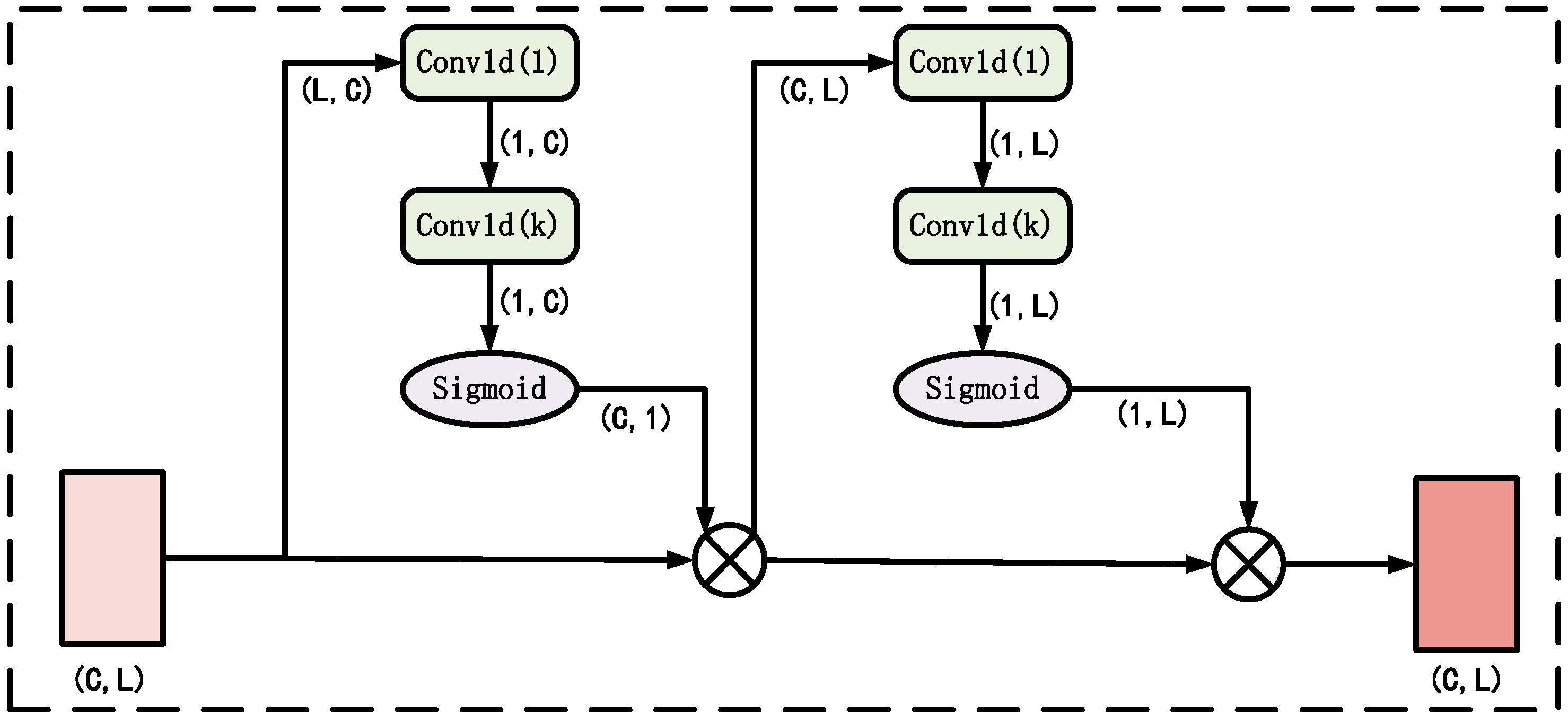
To enhance the model’s adaptive perception of critical features, a CBAM was incorporated into the network. This module comprises two components: Channel Attention (CA) and Spatial Attention (SA), which adaptively weight features along the channel and spatial dimensions, respectively, thereby improving feature representation, as illustrated in Figure 5.
Channel Attention (CA). The objective of the CA module is to adaptively recalibrate channel-wise feature importance. Given an input feature tensor: X R B × C × L , where B denotes batch size, C the number of channels, and L the feature length, the channel attention is computed as follows:
Channel Compression: The input is compressed along the channel dimension via a 1 × 1 convolution, yielding a single-channel representation:
X c = C o n v 1 d 1 × 1 X T
where X T R B × L × C denotes the transposed input tensor along the channel dimension.
Local Interaction Convolution: A 1D convolution is applied on the compressed single-channel feature to capture local inter-channel dependencies:
M c = C o n v 1 d k X c
The kernel size k is dynamically determined according to the number of input channels C:
t = log 2 C + 1 2 ,             k = t + 1 t m o d 2
where denotes the floor operation. This design ensures the convolution kernel adapts to the channel scale, remains odd-sized for symmetry in 1D convolution, and enlarges the attention receptive field.
Channel Attention Mapping: A Sigmoid activation generates the channel attention weights:
A c = σ M c 0,1 B × C × 1
Channel-Weighted Output: The input features are reweighted by the attention map:
X = X A c
Spatial Attention (SA). The SA module adaptively highlights the importance of features at specific positions in the sequence or spatial domain. Its computation proceeds as follows:
Channel Compression: Input features are compressed along the channel dimension to produce a single-channel spatial representation:
X s = C o n v 1 d 1 × 1 X
Local Spatial Convolution: A 1D convolution is applied on the compressed feature:
M s = C o n v 1 d k X s
Here, the kernel size k matches that of the CA module to maintain a consistent local receptive field.
Spatial Attention Mapping: A Sigmoid activation generates the spatial attention weights:
A s = σ M s 0,1 B × 1 × L
Spatial-Weighted Output: The final spatially reweighted output is obtained as:
X = X A s
The CBAM enhances feature representation through dual-dimensional attention, simultaneously considering channel-wise and spatial-wise importance to achieve multi-level feature weighting. By leveraging sigmoid-based weight mapping, it adaptively emphasizes critical features while suppressing redundancy, ensuring more informative representations. Its efficient and lightweight design, which relies solely on 1 × 1 and local convolutions without introducing additional fully connected parameters, makes it highly suitable for integration into deep convolutional networks. Overall, CBAM strengthens the model’s ability to focus on essential channels and spatial positions, thereby improving the accuracy of sequential feature extraction and representation.

2.3.6. Haar Wavelet Decomposition Module

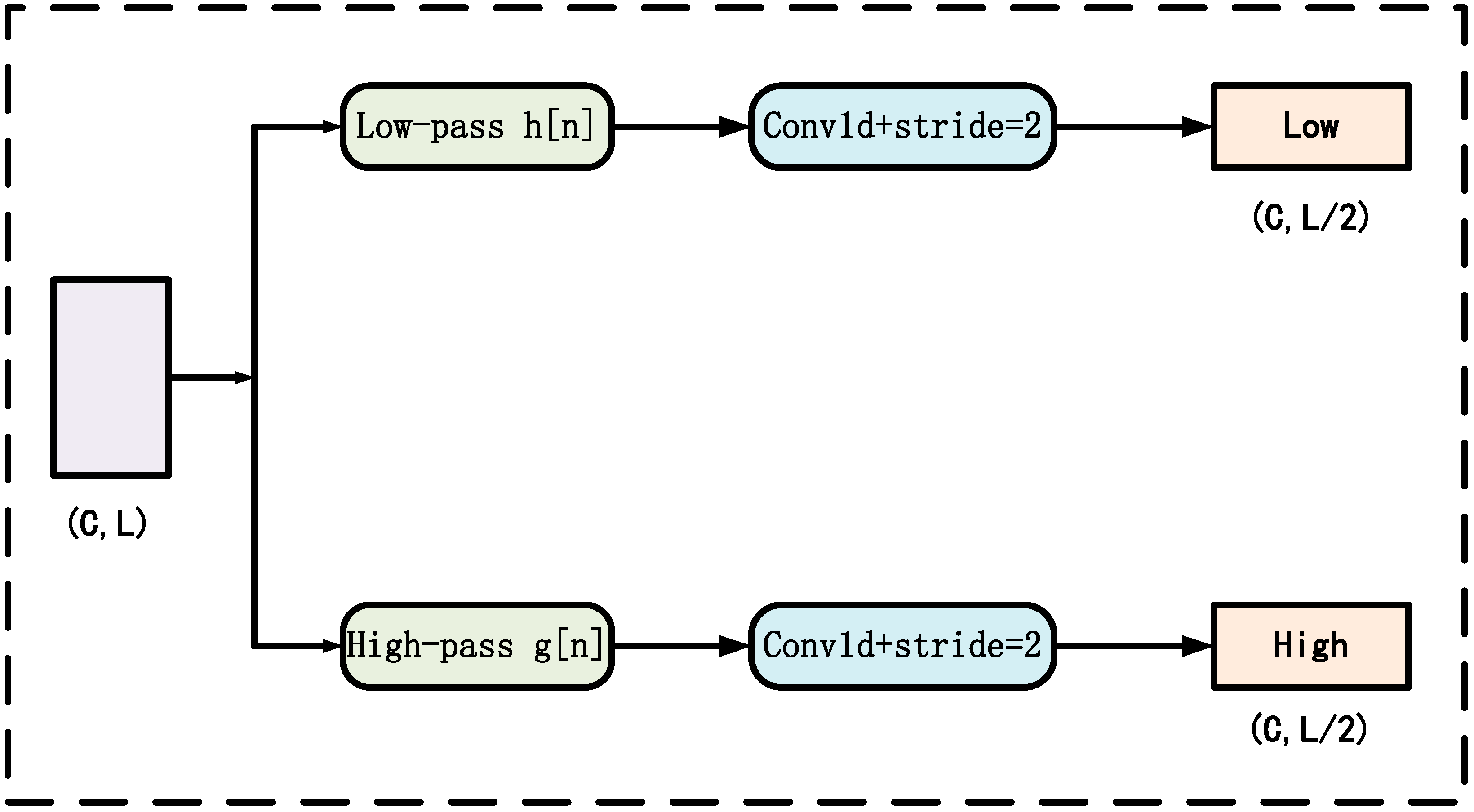
To simultaneously extract both low- and high-frequency information from sequential features, this study introduces a HWDM for multi-scale decomposition and feature enhancement. The module decomposes the input sequence into low-frequency approximation components and high-frequency detail components, thereby providing rich frequency-domain features for subsequent network processing, as illustrated in Figure 6.
Haar wavelet filter design. The Haar wavelet is one of the simplest and most widely used wavelets. Its one-dimensional discrete filters are defined as follows:
Low-pass filter (approximation component):
h [ n ] = 1 2 [ 1,1 ] ,             n = 0,1
High-pass filter (detail component):
g [ n ] = 1 2 [ 1 , 1 ] ,             n = 0,1
where 1 2 is the normalization factor that ensures energy preservation during the transform. The low-pass filter extracts smooth approximation features of the signal, while the high-pass filter captures rapid variations and detailed features.
Module implementation via convolution. Given an input feature tensor X R B × C × L , where B denotes the batch size, C the number of channels, and L the sequence length, the standard Haar wavelet decomposition module applies convolution independently to each channel:
X l o w = X h [ n ] ,             X h i g h = X g [ n ]
Here, denotes the convolution operation, and the stride is set to 2 to achieve downsampling, reducing the output sequence length by half. Since convolution is performed in a channel-wise manner (groups = C), each channel independently obtains its low- and high-frequency components.
Output feature representation. The module produces two components: X l o w , X h i g h R B × C × L 2 , X l o w is low-frequency approximation component, containing global trend information of the signal. X h i g h is high-frequency detail component, capturing rapid variations and edge features.
This decomposition not only facilitates the extraction of multi-scale features but also suppresses noise through the separation of low- and high-frequency components, thereby enhancing subsequent feature extraction and modeling.
The proposed HWDM exhibits several advantages. By decomposing the input into both low- and high-frequency components, it effectively captures multi-scale features, simultaneously providing global trend information and local detail representation. Its lightweight design relies solely on two-point convolutions with stride-based downsampling, avoiding additional parameters and maintaining low computational cost. Furthermore, channel-wise convolution ensures that features are independently extracted from each channel, making the module well-suited for multi-channel sequential inputs. Overall, this component offers an efficient way to extract frequency-domain decomposition features for deep neural networks and markedly improves their capacity to recognize multi-scale patterns in one-dimensional signals and temporal data.

2.4. Evaluation Metrics

To rigorously evaluate both the fitting accuracy and the generalization capacity of the soil spectral regression models, this study adopts six complementary statistical measures: the coefficient of determination (R2), root mean squared error (RMSE), mean absolute error (MAE), interquartile range (IQR), residual prediction deviation (RPD), and concordance correlation coefficient (CCC).
Together, these indicators describe goodness-of-fit, predictive precision, and stability from multiple viewpoints, thereby avoiding the bias that can arise when relying on a single metric.
The coefficient of determination (R2) expresses the proportion of variance in the observations explained by the model and is calculated as:
R 2 = 1 i = 1 n ( y i y ^ i ) 2 i = 1 n ( y i y ¯ ) 2
where y i is the measured value, y ^ i the predicted value, and y ¯ the sample mean. Values nearer to 1 reflect stronger explanatory power.
RMSE captures the overall deviation between predictions and measurements:
R M S E = 1 n i = 1 n ( y i y ^ i ) 2
Its unit matches that of the original data; smaller values correspond to higher predictive accuracy.
MAE quantifies the mean absolute discrepancy between predictions and observations:
M A E = 1 n i = 1 n | y i y ^ i |
Because it is less sensitive to extreme values, MAE provides a robust measure of average error.
The dispersion of prediction errors is summarized by the interquartile range:
I Q R = Q 3 Q 1
where Q 1 and Q 3 represent the 25th and 75th percentiles of the residuals. A smaller IQR indicates that errors are more tightly clustered.
Robustness is further examined with the residual prediction deviation:
R P D = S D R M S E
where S D is the standard deviation of the observed data. In spectral modeling, an RPD exceeding 2 typically signals good predictive ability.
Finally, the concordance correlation coefficient accounts for both correlation strength and systematic bias:
C C C = 2 ρ σ y σ y ^ σ y 2 + σ y ^ 2 + ( μ y μ y ^ ) 2
Here, ρ is the Pearson correlation coefficient, σ y and σ y ^ are the standard deviations of the observed and predicted values, and μ y and μ y ^ are their means. CCC values close to 1 denote stronger agreement.
By combining R2, RMSE, MAE, IQR, RPD and CCC, this analysis evaluates model performance from several perspectives (explanatory strength, error magnitude, error spread, robustness, and concordance), ensuring a thorough and scientifically rigorous assessment.

2.5. Experimental Setup

The experiments in this study were conducted on a workstation equipped with a 13th-generation Intel Core i7-13620H processor (10 cores/16 threads, base frequency 2.40 GHz; Intel, Santa Clara, CA, USA) and an NVIDIA GeForce RTX 4060 GPU (8 GB memory; NVIDIA, Santa Clara, CA, USA), with 16 GB of system RAM.
The software environment consisted of the Windows 11 operating system, the Python 3.12 programming language, and the PyTorch 2.6.0+cu124 deep learning framework. Under this configuration, each training epoch required approximately 1.21 s and consumed about 3.6 GB of GPU memory.
MAWC-Net contains 8,599,657 trainable parameters (approximately 32.8 MB), representing a moderately sized deep learning model suitable for efficient training on standard GPU hardware. Hyperparameters were selected through a grid search strategy, in which learning rate, batch size, and convolutional kernel settings were systematically explored based on validation performance.
For model training, the Adam optimizer was employed together with a cosine-annealing learning-rate scheduler. The initial learning rate was set to 7 × 10 5 , the batch size was 112, and the total number of training epochs was 500.

3. Results

3.1. Ablation Experiment

To evaluate the effectiveness of each key component in the proposed model, ablation experiments were conducted by progressively incorporating different structural units into the base network (BaseBlock). The added modules included the MSBCM, PAM, MSCDM, CBAM, and HWDM. Comparative experiments were performed on both the pH(CaCl2) and pH(H2O) datasets, and the results are summarized in Table 3 and Table 4.
As shown in Table 3, for the pH(CaCl2) prediction task, the BaseBlock alone achieved R2 = 0.940 with an RMSE of 0.346. Introducing the multi-scale convolution module (BaseBlock + MSBCM) significantly improved performance, increasing R2 to 0.944 and reducing RMSE to 0.335, demonstrating the effectiveness of the parallel multi-scale convolution structure in enhancing spectral feature extraction. Adding the path attention module (BaseBlock + MSBCM + PAM) further boosted discriminative ability, achieving R2 = 0.946 and RMSE = 0.329, which verifies the benefit of path-level feature weighting. The inclusion of the MSCDM and CBAM also yielded additional gains, with the combination of BaseBlock + MSCDM + CBAM reaching R2 = 0.947 and RMSE = 0.328. Ultimately, the proposed MAWC-Net, which integrates all modules, achieved the best results (R2 = 0.953, RMSE = 0.307, MAE = 0.214, RPD = 4.61, and CCC = 0.976), representing a substantial improvement over the base network.
A similar trend was observed for the pH(H2O) prediction task in Table 4. The BaseBlock achieved R2 = 0.929 and RMSE = 0.359. Incorporating the multi-scale convolution module raised R2 to 0.935 and reduced RMSE to 0.343, while adding PAM further enhanced performance to R2 = 0.938 and RMSE = 0.334. The MSCDM and CBAM combination also provided additional benefits, and the final MAWC-Net attained the best predictive performance (R2 = 0.945, RMSE = 0.315, MAE = 0.231, RPD = 4.28, and CCC = 0.972). These results confirm the effectiveness and robustness of the multi-module integration strategy for modeling soil pH.
In summary, the ablation experiments clearly demonstrate that the MSBCM strengthens spectral feature representation, the PAM effectively emphasizes critical information, and the MSCDM, CBAM, and HWDM each provide auxiliary improvements. The fully integrated MAWC-Net consistently delivers the best performance across different soil pH prediction tasks, validating both the rationality and superiority of the proposed network architecture.

3.2. Comparative Experiment

To further demonstrate the superiority of the proposed model, we compared MAWC-Net with several traditional machine learning algorithms and representative deep learning architectures. The baseline methods included Partial Least Squares Regression (PLSR), Ridge Regression (Ridge), Support Vector Regression (SVR), and XGBoost as traditional regression approaches, as well as VGG16, ResNet18, and CNN-Transformer as deep learning models. Experiments were conducted separately on the pH(CaCl2) and pH(H2O) datasets, and the results are summarized in Table 5 and Table 6. For deep learning models, we used grid search for hyperparameter tuning, while for traditional machine learning methods, we performed five-fold cross-validation-based hyperparameter optimization. All baseline models were trained using the same preprocessing pipeline to ensure a fair evaluation.
As shown in Table 5 (pH in CaCl2), traditional machine learning methods (PLSR, Ridge, and SVR) exhibited relatively weak performance, with R2 values around 0.87, RMSE values exceeding 0.50, and RPD values below 3, indicating their limited ability to capture the complex nonlinear characteristics of soil spectral sequences. XGBoost performed even worse, achieving only R2 = 0.722 and an RMSE as high as 0.752, suggesting difficulty in modeling high-dimensional spectral features. Deep learning models achieved clearly better results than traditional methods: among them, the CNN-Transformer reached R2 = 0.940 and RMSE = 0.346, representing a relatively strong baseline. The proposed MAWC-Net achieved the best overall performance, with R2 = 0.953, RMSE = 0.307, MAE = 0.214, RPD = 4.61, and CCC = 0.976, surpassing all comparison models.
A similar trend was observed for the pH(H2O) dataset in Table 6. Traditional methods (PLSR, Ridge, SVR) delivered limited predictive accuracy, with the highest R2 reaching only 0.877 and RMSE around 0.474. XGBoost again performed poorly (R2 = 0.723, RMSE = 0.713). Deep learning models outperformed traditional approaches overall, with CNN-Transformer showing the best performance among them (R2 = 0.932, RMSE = 0.352). MAWC-Net once again achieved the most accurate results, obtaining R2 = 0.945, RMSE = 0.315, MAE = 0.231, RPD = 4.28, and CCC = 0.972, demonstrating its robustness and strong generalization capability for spectral modeling tasks.
In summary, these comparative experiments reveal that traditional statistical modeling methods have limited predictive power due to their inability to capture the nonlinear and multi-scale characteristics of soil spectra. Classic deep learning networks improve performance to some extent but still struggle with sufficient feature extraction. By integrating multi-scale convolution and attention mechanisms, the proposed MAWC-Net effectively enhances spectral feature representation and key-channel modeling, achieving consistently superior results on both datasets and fully validating the rationality and advanced nature of its architectural design. In addition, we provide a comparison of model sizes to further ensure fairness in evaluation: VGG16 contains 138,357,544 parameters (528 MB), ResNet18 contains 11,689,512 parameters (44.6 MB), CNN-Transformer contains 11,708,481 parameters (44.7 MB), whereas the proposed MAWC-Net contains only 8,599,657 parameters (32.8 MB). This demonstrates that the superior performance of MAWC-Net is not attributable to a larger parameter count but rather to its efficient and well-designed multi-scale and attention-based architecture.

3.3. Robustness and Reproducibility Verification

During the training of deep learning models, variations in random seeds can affect parameter initialization, sample partitioning, and optimization paths, potentially leading to differences in model outcomes. To evaluate the robustness and reproducibility of the proposed model under different random seeds, thirty seeds were randomly selected from the range 0–1000. The model’s performance was then assessed on the pH(CaCl2) and pH(H2O) prediction tasks, and the root mean square error (RMSE) on the test sets was recorded.
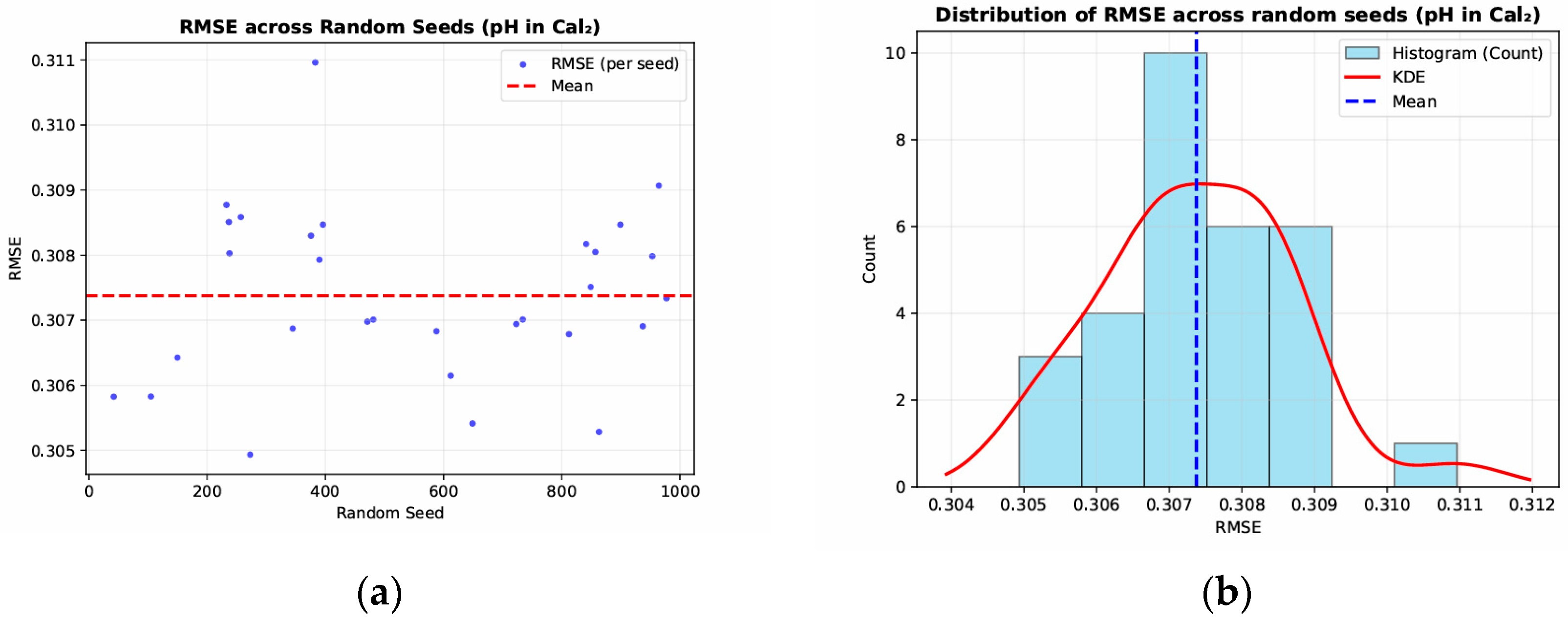
The variations and distributions of RMSE across different random seeds are presented in Figure 7. The results indicate that:
  • Overall Stability: For pH(CaCl2), the average RMSE was approximately 0.307, with values ranging roughly from 0.305 to 0.311. For pH(H2O), the mean RMSE was around 0.315, fluctuating between approximately 0.311 and 0.316. The minimal variation across different random seeds indicates that the model maintains consistent performance in repeated trials.
  • Distribution Concentration: The RMSE histograms and kernel density estimation (KDE) curves exhibit an approximately normal shape, with the mean closely matching the mode. This pattern further supports that the model’s predictive accuracy is largely independent of the choice of random seed.
  • Robustness Assessment: Across repeated experiments for both pH(CaCl2) and pH(H2O), no extreme outliers or abrupt deviations were observed. This demonstrates that the model remains stable and robust under varying initialization conditions, highlighting its strong generalization ability and minimizing the influence of random factors on predictive outcomes.
In summary, the repeated experiments confirm that the proposed model exhibits excellent robustness and reproducibility in soil pH prediction tasks, providing a solid foundation for subsequent practical applications and broader deployment.

4. Discussion

4.1. Further Analysis and Evaluation of Experimental Results

The experimental findings, as shown in Figure 8, demonstrate that the proposed model achieved excellent performance in predicting soil pH. Under the CaCl2 extract condition, the predicted values exhibited a high correlation with the measured values, yielding a coefficient of determination (R2) of 0.953 and a root mean square error (RMSE) of only 0.307. Under the H2O extract condition, the model also performed exceptionally well, with R2 reaching 0.945 and RMSE at 0.315. Scatter plots clearly show that the predicted and measured values are closely distributed along the y = x diagonal, and the fitted regression line is nearly identical to the ideal fit line, indicating strong fitting capability and robust generalization.
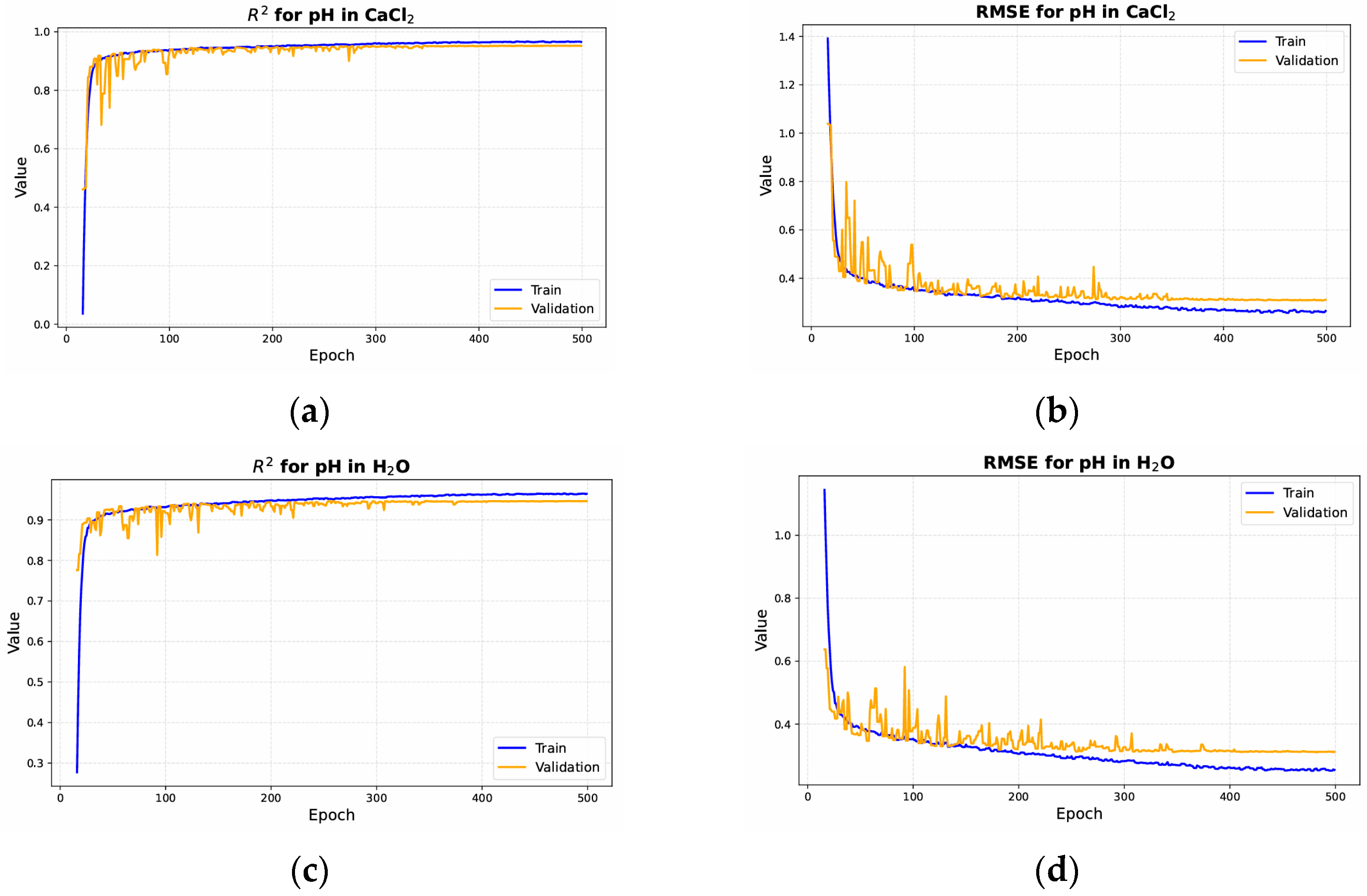
The training process, as illustrated in Figure 9, further confirmed the model’s effectiveness. From the R2 curves of the training and validation sets, both rapidly increased and stabilized as the number of epochs grew, maintaining high levels after approximately 100 epochs. This indicates that the model converges quickly while sustaining stable predictive accuracy. Meanwhile, the RMSE curves exhibited a rapid decline before stabilizing, showing only minor fluctuations on the validation set and no evidence of overfitting. This behavior further confirms the model’s stable performance and robustness across different datasets.
Overall, the experimental outcomes demonstrate that the proposed model achieves high accuracy and stability in predicting soil pH. Compared with conventional approaches, the deep learning framework more effectively captures the complex nonlinear relationships present in spectral data, leading to substantial improvements in predictive performance. In addition, the minimal differences observed between predictions under CaCl2 and H2O extraction conditions indicate that the model exhibits strong adaptability and generalization across different measurement protocols. These results offer a reliable technical basis for soil nutrient assessment and support large-scale soil monitoring efforts.

4.2. Method Advantages and Limitations

The proposed MAWC-Net model exhibits notable advantages in soil spectral modeling, owing to the complementary effects of its specialized modules:
  • Multi-scale Feature Extraction: The multi-scale convolution strategy is well suited for one-dimensional spectral data without an explicit temporal dimension. Parallel convolutions with different kernel sizes (e.g., 3, 5, 7, 9) allow the network to extract features at multiple receptive fields, capturing both narrow absorption peaks and broader spectral patterns. In contrast, Transformer architectures are primarily designed for sequential data with temporal dependencies, where self-attention mechanisms dynamically model long-range interactions. In the attention-based study [32], the core architecture relies on heavy self-attention mechanisms. In the Transformer-based study [33], the primary modeling component is again the Transformer with multi-head self-attention. When using a Transformer architecture, the multi-head self-attention mechanism is an essential component. In self-attention, the input features must be projected into query (Q), key (K), and value (V) matrices through separate learned linear transformations. The attention operation then computes QKT followed by a softmax normalization and a weighted multiplication with V. These steps involve multiple large matrix multiplications, and in the multi-head setting, they are repeated across several attention heads. As a result, the computational cost grows significantly, leading to substantial memory usage and increased runtime complexity. During our preliminary experiments, we also evaluated self-attention modules, but the computational overhead was prohibitive given the limitations of our hardware. Therefore, we focused on computationally efficient alternatives that still retain strong representational capacity.
  • Attention Mechanisms: The network employs PAM and CBAM to perform adaptive feature weighting across multiple layers. PAM selectively emphasizes informative feature paths, while CBAM adaptively reweights feature channels and spatial locations. These attention mechanisms help the model focus on relevant spectral and spatial information, thereby enhancing feature representation and supporting improved predictive accuracy and generalization.
  • Frequency-Domain Information Enhancement: The model incorporates a HWDM to project time-domain features into low- and high-frequency sub-bands. By processing these sub-bands separately, the model captures fine-grained frequency-domain variations, enhancing feature representation and supporting more robust and reliable predictions.
  • Practical Implications: In practical soil-sensing scenarios, MAWC-Net demonstrates strong potential for rapid and accurate pH estimation, which is valuable for precision agriculture, soil fertility assessment, and field-scale monitoring. These findings suggest that MAWC-Net can serve as a promising tool for real-time or near-real-time soil analysis, although future lightweighting or model compression may be required for deployment on portable spectrometers.
Despite these advantages, MAWC-Net also has certain limitations:
  • Interpretability: Although multiple attention mechanisms enhance critical spectral regions, the overall decision-making process remains difficult to interpret due to the network’s structural complexity. The coupling of different modules (e.g., the combined effects of CBAM and PAM) improves performance but makes it challenging to explicitly identify which spectral bands play a dominant role in prediction. In soil spectral modeling, this reduced interpretability may limit the model’s ability to provide mechanistic insights.
  • Model Lightweighting: While the design partially addresses model efficiency through MSCDM, MAWC-Net still integrates multi-scale convolutions, attention mechanisms, and wavelet decomposition. In resource-constrained scenarios (e.g., portable spectrometers or real-time analysis on mobile devices), model deployment may therefore be restricted. Future work should explore model compression and lightweight strategies to enhance applicability while maintaining predictive accuracy.
  • Prediction biases: Some prediction biases were observed for soils with extreme pH values or atypical spectral characteristics. These deviations may arise from multiple factors, including the intrinsic difficulty of modeling extreme chemical conditions, variations introduced during hyperspectral acquisition (e.g., illumination, soil moisture, sample heterogeneity), or occasional measurement noise caused by instrument calibration and sample preparation. Understanding these failure patterns provides useful guidance for improving dataset diversity, refining preprocessing procedures, and enhancing the robustness of future model designs.

5. Conclusions

In response to the challenges of insufficient multi-scale feature extraction, limited effective feature selection, and suboptimal generalization in soil spectral modeling, this study proposes a Multi-Scale Attention Wavelet Convolutional Neural Network (MAWC-Net). The model integrates multi-scale convolution modules, PAM, CBAM, and HWDM to achieve hierarchical spectral feature modeling and efficient feature selection.
Experiments conducted on the LUCAS2009 dataset lead to the following main conclusions:
  • Superior predictive accuracy: The proposed MAWC-Net significantly outperforms both traditional statistical approaches and existing deep learning models in soil pH prediction, achieving higher coefficients of determination (R2) and lower root mean squared errors (RMSEs). These results confirm the effectiveness of combining multi-scale convolution with attention mechanisms.
  • Necessity of each module: Ablation studies demonstrate that removing key components—such as the multi-scale convolution, attention mechanisms, or wavelet decomposition—consistently degrades model performance. This finding highlights the synergistic contribution of the overall network architecture to feature extraction and enhancement.
  • Strong generalization and robustness: Comparative experiments and robustness tests show that MAWC-Net maintains stable predictive performance across different dataset partitions and random seed settings, indicating high reliability and robustness for soil spectral modeling.
  • Areas for improvement in interpretability and lightweight design: Despite its superior accuracy, the model’s structural complexity limits mechanistic interpretability and deployment in resource-constrained environments. Future work should incorporate explainable-AI methods and model compression techniques to enhance the scientific interpretability and practical applicability of MAWC-Net.
In summary, the proposed MAWC-Net demonstrates high predictive accuracy and robustness for soil spectral modeling, offering a new approach for rapid and accurate prediction of soil physicochemical properties and providing a foundation for future applications in agriculture, environmental monitoring, and related fields.

Author Contributions

Conceptualization, X.C., Z.L., X.X. and Y.D.; methodology, X.C. and Z.L.; software, X.C. and Z.L.; validation, X.C., Z.L., Q.L. and Y.K.; formal analysis, X.C., Z.L., J.T., Y.S. and J.Z.; investigation, Z.L. and Y.D.; resources, X.C., X.X. and Y.D.; data curation, Z.L. and J.T.; writing—original draft preparation, X.C. and Z.L.; writing—review and editing, X.C., Z.L., X.X., Y.D., Q.L., Y.K., J.T., Y.S. and J.Z.; supervision, X.C.; project administration, X.C.; funding acquisition, X.C. All authors have read and agreed to the published version of the manuscript.

Funding

This research work was supported by Key R & D projects of Guangxi Science and Technology Program (Guike.AB24010338), The central government guides local science and technology development fund projects (GuikeZY22096012), National natural science foundation of China (32360374), and Independent research project (GXRDCF202307-01).

Institutional Review Board Statement

Not applicable.

Informed Consent Statement

Not applicable.

Data Availability Statement

Data and access to the public dataset LUCAS are available at the following link: https://esdac.jrc.ec.europa.eu/projects/lucas (accessed on 29 July 2025).

Acknowledgments

The authors sincerely thank all the researchers who participated in the experiments for their valuable efforts and contributions. The financial support from the relevant institutions is gratefully acknowledged. The authors also declare that no artificial intelligence tools were used to fabricate, manipulate, or generate any experimental data or results presented in this study.

Conflicts of Interest

The authors declare no conflicts of interest.

References

  1. Yunta, F.; Schillaci, C.; Panagos, P.; Van Eynde, E.; Wojda, P.; Jones, A. Quantitative analysis of the compliance of EU Sewage Sludge Directive by using the heavy metal concentrations from LUCAS topsoil database. Environ. Sci. Pollut. Res. 2025, 32, 16554–16569. [Google Scholar] [CrossRef] [PubMed]
  2. Zamanian, K.; Taghizadeh-Mehrjardi, R.; Tao, J.; Fan, L.; Raza, S.; Guggenberger, G.; Kuzyakov, Y. Acidification of European croplands by nitrogen fertilization: Consequences for carbonate losses, and soil health. Sci. Total Environ. 2024, 924, 171631. [Google Scholar] [CrossRef]
  3. Geng, Y.; Zhou, T.; Zhang, Z.; Cui, B.; Sun, J.; Zeng, L.; Yang, R.; Wu, N.; Liu, T.; Pan, J.; et al. Continental-scale mapping of soil pH with SAR-optical fusion based on long-term earth observation data in google earth engine. Ecol. Indic. 2024, 165, 112246. [Google Scholar] [CrossRef]
  4. Park, S.; Jeon, S.; Kwon, N.H.; Kwon, M.; Shin, J.H.; Kim, W.C.; Lee, J.G. Application of near-infrared spectroscopy to predict chemical properties in clay rich soil: A review. Eur. J. Agron. 2024, 159, 127228. [Google Scholar] [CrossRef]
  5. Piccini, C.; Metzger, K.; Debaene, G.; Stenberg, B.; Götzinger, S.; Boruvka, L.; Sandén, T.; Bragazza, L.; Liebisch, F. In-field soil spectroscopy in Vis–NIR range for fast and reliable soil analysis: A review. Eur. J. Soil Sci. 2024, 75, e13481. [Google Scholar] [CrossRef]
  6. Sun, W.; Liu, S.; Jiang, L.; Zhou, B.; Zhang, X.; Shang, K.; Jiang, W.; Jiang, Z. Prediction and monitoring of soil pH using field reflectance spectroscopy and time-series Sentinel-2 remote sensing imagery. Geomatica 2025, 77, 100053. [Google Scholar] [CrossRef]
  7. Gözükara, G. Vis-NIR ve pXRF Spektrometrelerinin Toprak Biliminde Kullanımı. Türkiye Tarımsal Araştırmalar Derg. 2021, 8, 125–132. [Google Scholar] [CrossRef]
  8. Wang, Z.; Chen, S.; Lu, R.; Zhang, X.; Ma, Y.; Shi, Z. Non-linear memory-based learning for predicting soil properties using a regional vis-NIR spectral library. Geoderma 2024, 441, 116752. [Google Scholar] [CrossRef]
  9. Hosseinpour-Zarnaq, M.; Omid, M.; Sarmadian, F.; Ghasemi-Mobtaker, H. A CNN model for predicting soil properties using VIS–NIR spectral data. Environ. Earth Sci. 2023, 82, 382. [Google Scholar] [CrossRef]
  10. Zhang, Y.; Cheng, G.; He, L. Convolutional Neural networks based on parallel multi-scale pooling branch: A transfer diagnosis method for mechanical vibrational signal with less computational cost. Measurement 2022, 192, 110905. [Google Scholar] [CrossRef]
  11. Lei, T.; Sun, D.W. Achieving joint calibration of soil Vis-NIR spectra across instruments, soil types and properties by an attention-based spectra encoding-spectra/property decoding architecture. Geoderma 2022, 405, 115449. [Google Scholar] [CrossRef]
  12. Jin, X.; Zhou, J.; Rao, Y.; Zhang, X.; Zhang, W.; Ba, W.; Zhou, X.; Zhang, T. An innovative approach for integrating two-dimensional conversion of Vis-NIR spectra with the Swin Transformer model to leverage deep learning for predicting soil properties. Geoderma 2023, 436, 116555. [Google Scholar] [CrossRef]
  13. Feng, G.; Li, Z.; Zhang, J.; Wang, M. Multi-Scale Spatial Attention-Based Multi-Channel 2D Convolutional Network for Soil Property Prediction. Sensors 2024, 24, 4728. [Google Scholar] [CrossRef]
  14. Saberioon, M.; Gholizadeh, A.; Ghaznavi, A.; Chabrillat, S.; Khosravi, V. Enhancing soil organic carbon prediction of LUCAS soil database using deep learning and deep feature selection. Comput. Electron. Agric. 2024, 227, 109494. [Google Scholar] [CrossRef]
  15. Liu, Y.; Shen, L.; Zhu, X.; Xie, Y.; He, S. Spectral data-driven prediction of soil properties using LSTM-CNN-attention model. Appl. Sci. 2024, 14, 11687. [Google Scholar] [CrossRef]
  16. Fu, X.; Leng, G.; Zhang, Z.; Huang, J.; Xu, W.; Xie, Z.; Wang, Y. Enhancing soil nitrogen measurement via visible-near infrared spectroscopy: Integrating soil particle size distribution with long short-term memory models. Spectrochim. Acta Part A Mol. Biomol. Spectrosc. 2025, 327, 125317. [Google Scholar] [CrossRef] [PubMed]
  17. Zhu, J.; Wang, W.; Tian, P. Spectroscopic measurement of near-infrared soil pH parameters based on GhostNet-CBAM. PLoS ONE 2025, 20, e0325426. [Google Scholar] [CrossRef]
  18. Cao, L.; Yin, D.; Sun, M.; Yang, Y.; Hassan, M.; Duan, Y. ResHAN-GAM: A novel model for the inversion and prediction of soil organic matter content. Ecol. Inform. 2025, 90, 103192. [Google Scholar] [CrossRef]
  19. Deng, Y.; Cao, Y.; Chen, S.; Cheng, X. Residual Attention Network with Atrous Spatial Pyramid Pooling for Soil Element Estimation in LUCAS Hyperspectral Data. Appl. Sci. 2025, 15, 7457. [Google Scholar] [CrossRef]
  20. Wang, X.; Zhang, M.W.; Zhou, Y.N.; Wang, L.; Zeng, L.T.; Cui, Y.P.; Sun, X.L. Simultaneous estimation of multiple soil properties from vis-NIR spectra using a multi-gate mixture-of-experts with data augmentation. Geoderma 2025, 453, 117127. [Google Scholar] [CrossRef]
  21. Tong, Z.; Liu, L. SpatialFormer: A Model to Estimate Soil Organic Carbon Content Using Spectral and Spatial Information. J. Soil Sci. Plant Nutr. 2025, 25, 3259–3271. [Google Scholar] [CrossRef]
  22. Li, C.; Song, L.; Zheng, L.; Ji, R. DSCformer: Lightweight model for predicting soil nitrogen content using VNIR-SWIR spectroscopy. Comput. Electron. Agric. 2025, 230, 109761. [Google Scholar] [CrossRef]
  23. Leenen, M.; Pätzold, S.; Tóth, G.; Welp, G. A LUCAS-based mid-infrared soil spectral library: Its usefulness for soil survey and precision agriculture. J. Plant Nutr. Soil Sci. 2022, 185, 370–383. [Google Scholar] [CrossRef]
  24. Clingensmith, C.M.; Grunwald, S. Predicting soil properties and interpreting Vis-NIR models from across continental United States. Sensors 2022, 22, 3187. [Google Scholar] [CrossRef] [PubMed]
  25. Paheding, S.; Reyes, A.A.; Kasaragod, A.; Oommen, T. GAF-NAU: Gramian Angular Field encoded Neighborhood Attention U-Net for Pixel-Wise Hyperspectral Image Classification. In Proceedings of the 2022 IEEE/CVF Conference on Computer Vision and Pattern Recognition Workshops (CVPRW), New Orleans, LA, USA, 19–20 June 2022; pp. 408–416. [Google Scholar]
  26. Nai, H.; Zhang, C.; Hu, X. Enhancing the Distinguishability of Minor Fluctuations in Time Series Classification Using Graph Representation: The MFSI-TSC Framework. Sensors 2025, 25, 4672. [Google Scholar] [CrossRef]
  27. Thomas, F.; Petzold, R.; Landmark, S.; Mollenhauer, H.; Becker, C.; Werban, U. Estimating Forest Soil Properties for Humus Assessment—Is Vis-NIR the Way to Go? Remote Sens. 2022, 14, 1368. [Google Scholar] [CrossRef]
  28. Javadi, S.H.; Mouazen, A.M. Data fusion of XRF and Vis-nir using outer product analysis, granger–Ramanathan, and least squares for prediction of key soil attributes. Remote Sens. 2021, 13, 2023. [Google Scholar] [CrossRef]
  29. Rendleman, M.C.; Smith, B.J.; Canahuate, G.; Braun, T.A.; Buatti, J.M.; Casavant, T.L. Representative random sampling: An empirical evaluation of a novel bin stratification method for model performance estimation. Stat. Comput. 2022, 32, 101. [Google Scholar] [CrossRef]
  30. Wilimitis, D.; Walsh, C.G. Practical considerations and applied examples of cross-validation for model development and evaluation in health care: Tutorial. JMIR AI 2023, 2, e49023. [Google Scholar] [CrossRef]
  31. Szeghalmy, S.; Fazekas, A. A comparative study of the use of stratified cross-validation and distribution-balanced stratified cross-validation in imbalanced learning. Sensors 2023, 23, 2333. [Google Scholar] [CrossRef]
  32. Wang, S. Evaluating cross-building transferability of attention-based automated fault detection and diagnosis for air handling units: Auditorium and hospital case study. Build. Environ. 2025, 287, 113889. [Google Scholar] [CrossRef]
  33. Wang, S. A hybrid SMOTE and Trans-CWGAN for data imbalance in real operational AHU AFDD: A case study of an auditorium building. Energy Build. 2025, 348, 116447. [Google Scholar] [CrossRef]
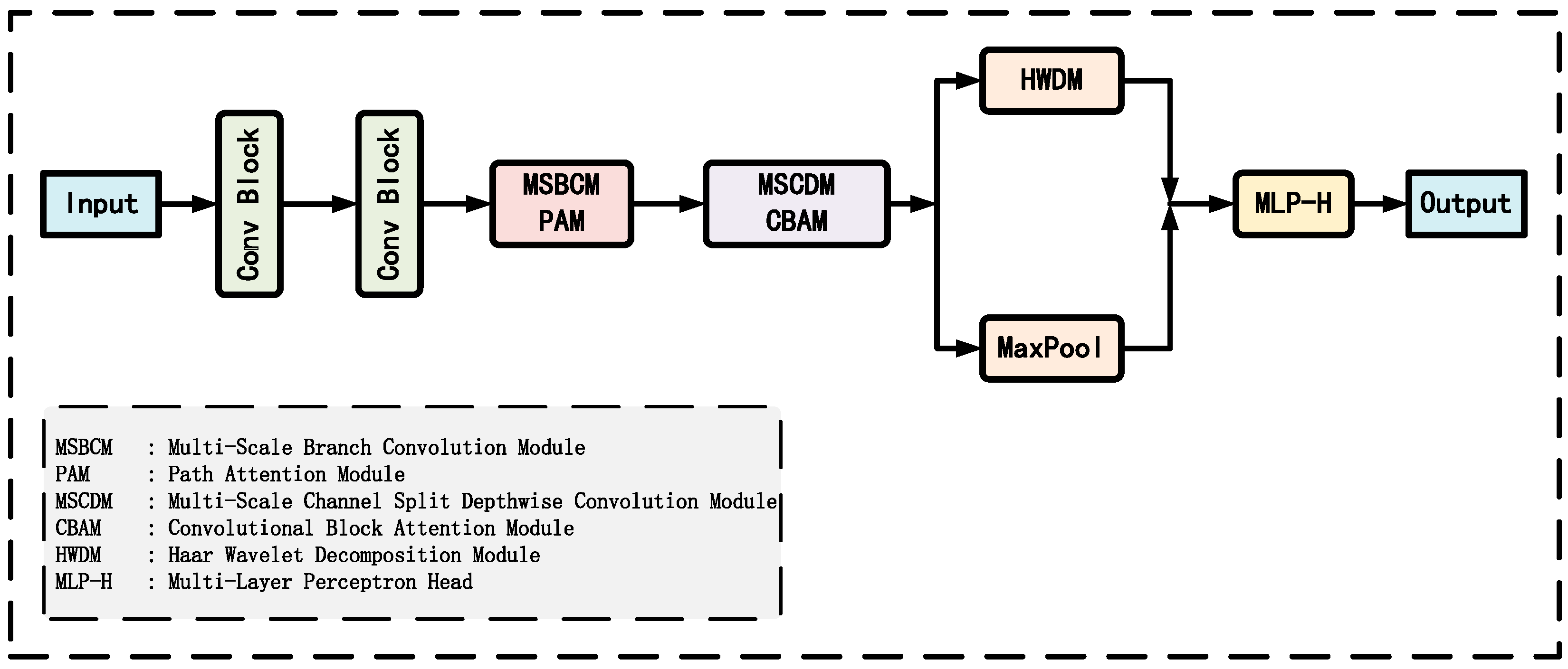
Figure 1. Overall Model Architecture.
Applsci 16 00054 g001
Figure 2. Multi-Scale Branch Convolution Module.
Applsci 16 00054 g002
Figure 3. Path Attention Module.
Applsci 16 00054 g003
Figure 4. Multi-Scale Channel Split Depthwise Convolution Module.
Applsci 16 00054 g004
Figure 5. Convolutional Block Attention Module.
Applsci 16 00054 g005
Figure 6. Haar Wavelet Decomposition Module.
Applsci 16 00054 g006
Figure 7. RMSE results across different random seeds for soil pH: (a) pH in CaCl2, RMSE values per seed; (b) corresponding RMSE distribution (pH in CaCl2); (c) pH in H2O, RMSE values per seed; (d) corresponding RMSE distribution (pH in H2O).
Applsci 16 00054 g007aApplsci 16 00054 g007b
Figure 8. (a) Scatter plot of observed vs. predicted values for pH in CaCl2. (b) Scatter plot of observed vs. predicted values for pH in H2O.
Applsci 16 00054 g008
Figure 9. Training performance metrics across epochs for soil pH: (a) R2 for pH in CaCl2; (b) RMSE for pH in CaCl2; (c) R2 for pH in H2O; (d) RMSE for pH in H2O.
Applsci 16 00054 g009
Table 1. Statistical characteristics of soil pH datasets.
ElementSetSizeMeanStdIQRMedianKurtosis
pH in CaCl2Complete19,0365.591.432.685.64−1.30
SG19,0365.591.432.685.64−1.30
PAA19,0365.591.432.685.64−1.30
Mahalanobis18,0845.601.422.675.65−1.30
Train96445.601.422.675.64−1.30
Val24125.601.412.665.66−1.30
Test60285.601.422.675.65−1.30
pH in H2OComplete19,0366.201.352.456.21−1.24
SG19,0366.201.352.456.21−1.24
PAA19,0366.201.352.456.21−1.24
Mahalanobis18,0846.201.352.446.21−1.23
Train96446.201.352.446.20−1.23
Val24126.211.352.456.22−1.24
Test60286.201.352.446.21−1.23
Table 2. Network configuration of the MAWC-Net.
Module/BlockTypeOutputParameter Setting
InputInput[BS, 1, 128]
ConvConv1d[BS, 32, 128]kernel_size = 3, filters = 32
BatchNorm1d[BS, 32, 128]
Sigmoid[BS, 32, 128]
ConvConv1d[BS, 32, 128]kernel_size = 3, filters = 32
BatchNorm1d[BS, 32, 128]
Sigmoid[BS, 32, 128]
MSBCM (k = 3,5,7,9)4 parallel branches
Per-branchConv1d[BS, 64, 128]kernel_size∈{3,5,7,9}, filters = 64, padding = ⌊k/2⌋
BatchNorm1d[BS, 64, 128]
Sigmoid[BS, 64, 128]
PAM [BS, 64, 128]Path Attention Module
MSCDM (k = 3,5,7,9)4 parallel branches
Per-branchConv1d[BS, 32, 128]kernel_size∈{3,5,7,9}, filters = 32, padding = ⌊k/2⌋, group = 16
BatchNorm1d[BS, 32, 128]
CBAM[BS, 32, 128]
Conv1d[BS, 32, 128]kernel_size = 1, filters = 32
BatchNorm1d[BS, 32, 128]
Fusion LayerConv1d[BS, 128, 128]kernel_size = 1, filters = 128
BatchNorm1d[BS, 128, 128]
Sigmoid[BS, 128, 128]
MaxPoolMaxPool1d[BS, 128, 64]kernel_size = 2, stride = 2
HWDM [BS, 128, 64]×2Low-frequency + High-frequency
MLP-HLinear[BS, 1024]
BatchNorm1d[BS, 1024]
Sigmoid[BS, 1024]
Dropout[BS, 1024]dropout = 0.2
Linear[BS, 128]
BatchNorm1d[BS, 128]
Sigmoid[BS, 128]
Linear[BS, 1]
Table 3. Results of Ablation Studies for pH in CaCl2.
ModelR2RMSEMAEIQRRPDCCC
BaseBlock0.9400.3460.2420.2514.100.970
BaseBlock + MSBCM0.9440.3350.2330.2394.230.972
BaseBlock + MSBCM + PAM0.9460.3290.2300.2394.310.973
BaseBlock + MSCDM0.9430.3370.2300.2394.210.971
BaseBlock + MSCDM + CBAM0.9470.3280.2270.2314.330.973
BaseBlock + HWDM0.9430.3370.2360.2484.200.971
MAWC-Net0.9530.3070.2140.2184.610.976
Table 4. Results of Ablation Studies for pH in H2O.
ModelR2RMSEMAEIQRRPDCCC
BaseBlock0.9290.3590.2650.2683.750.964
BaseBlock + MSBCM0.9350.3430.2520.2553.920.967
BaseBlock + MSBCM + PAM0.9380.3340.2460.2534.030.969
BaseBlock + MSCDM0.9350.3440.2540.2603.920.967
BaseBlock + MSCDM + CBAM0.9380.3360.2470.2494.010.968
BaseBlock + HWDM0.9330.3480.2580.2633.870.966
MAWC-Net0.9450.3150.2310.2354.280.972
Table 5. pH in CaCl2 comparison table.
ModelR2RMSEMAEIQRRPDCCC
PLSR0.8710.5120.3940.4082.780.932
Ridge0.8700.5130.3940.4062.780.931
SVR0.8710.5110.3560.3722.790.934
XGBoost0.7220.7520.5860.6141.900.836
VGG160.9350.3600.2540.2623.930.967
ResNet180.9270.3820.2700.2873.710.963
CNN-Transformer0.9400.3460.2440.2524.090.969
MAWC-Net0.9530.3070.2140.2184.610.976
Table 6. pH in H2O comparison table.
ModelR2RMSEMAEIQRRPDCCC
PLSR0.8610.5040.3910.3992.690.927
Ridge0.8610.5050.3920.3982.680.926
SVR0.8770.4740.3600.3732.860.936
XGBoost0.7230.7130.5570.5781.900.837
VGG160.9260.3670.2730.2853.670.962
ResNet180.9180.3860.2850.2973.490.958
CNN-Transformer0.9320.3520.2610.2673.830.965
MAWC-Net0.9450.3150.2310.2354.280.972
Disclaimer/Publisher’s Note: The statements, opinions and data contained in all publications are solely those of the individual author(s) and contributor(s) and not of MDPI and/or the editor(s). MDPI and/or the editor(s) disclaim responsibility for any injury to people or property resulting from any ideas, methods, instructions or products referred to in the content.