Laplacian Manifold Learning Based Vibro-Acoustic Feature Fusion for Rail Corrugation Condition Characterization

Featured Application

The method proposed in this study is designed for rail corrugation monitoring under small-sample and weak-label conditions, and it can be directly applied to onboard real-time monitoring systems. While it is practically applicable to urban rail transit, the method can also be extended to rail corrugation monitoring in high-speed and heavy-haul railways, enabling generalized monitoring capability across different lines and scenarios.

Abstract

Accurate characterization of rail corrugation is essential for the operation and maintenance of urban rail transit. To enhance the representation capability for rail corrugation, this study proposes a sound–vibration feature fusion method based on Laplacian manifold learning. The method constructs a multidimensional feature space using real-world acoustic and vibration signals measured from metro vehicles, introduces a Laplacian manifold structure to capture local geometric relationships among samples, and incorporates inter-class separability into traditional intra-class compactness metrics. Based on this, a comprehensive feature evaluation index L_r is developed to achieve adaptive feature ranking. The final fusion indicator, LWVAF, is generated through weighted feature integration and used for rail corrugation characterization. Validation on in-service metro line data demonstrates that, after rail grinding, LWVAF exhibits a more pronounced reduction and higher sensitivity to changes compared with individual acoustic or vibration features, reliably reflecting improvements in rail corrugation. The results confirm that the proposed method maintains strong robustness and physical interpretability even under small-sample and weak-label conditions, offering a new approach for sound–vibration fusion analysis and corrugation evolution studies.

1. Introduction

Rail corrugation is a common wheel–rail contact fatigue and uneven wear defect in urban rail transit [1,2,3,4]. It not only increases vehicle noise, reduces ride comfort, and generates more passenger complaints, but also induces high-frequency vibrations in the vehicle–track system [5,6,7], accelerating fatigue damage of critical wheel–rail components and increasing maintenance costs and frequency [8,9,10]. With the continuous expansion of urban rail networks and the increasing service life of lines, noise and vibration issues have received growing attention. Therefore, monitoring rail corrugation and evaluating grinding effectiveness have become essential tasks in rail maintenance and operation.

Currently, rail corrugation detection mainly relies on two approaches: (1) contact-based measurement methods, such as track inspection trolleys [11,12,13], which can obtain high-precision geometric features of corrugation, including wavelength and depth. However, these methods have long inspection cycles, are labor-intensive, costly, and often require nighttime operation, making them unsuitable for high-frequency monitoring. (2) Online monitoring based on vehicle vibration signals [14,15,16], which infer track irregularities from acceleration responses during train operation. This approach offers real-time capability and convenient data acquisition, but vibration responses are sensitive to vehicle structure, suspension system, and operating speed. Consequently, response variations under different vehicle types or track conditions limit the stability of detection results.

Beyond vibration signals, recent studies have explored the sensitivity of acoustic signals to high-frequency vehicle–track responses and their potential application in onboard real-time monitoring. Zhang [17] analyzed the correlation between high-speed rail rail roughness and in-train noise, showing that corrugation features are prominently reflected in operational noise. Wei [18] utilized onboard noise collected during train operation to diagnose rail corrugation in high-speed railways. Liu [19] applied a wavelet packet-based feature extraction method on wheel–rail noise for rapid evaluation of corrugation amplitude. Han [20] constructed diagnostic indices based on the energy ratio of intrinsic mode components in acoustic signals, effectively identifying corrugation conditions. These studies indicate that acoustic signals, as a physical quantity directly accessible in a “vehicle–onboard platform–real-time acquisition–online analysis” framework, possess unique advantages in rail condition characterization. However, acoustic signals are also prone to environmental noise interference, limiting the stability of characterization when used alone.

To overcome the limitations of single acoustic or vibration signals, sound–vibration fusion has gradually become an important research direction in rail structural health monitoring. By integrating complementary information from acoustic and vibration signals, more robust rail condition recognition can be achieved at the feature, decision, or model level. Wang [21] proposed a rail corrugation characterization index based on sound–vibration fusion for metro tracks. Huang [22] and Cong [23] designed corrugation identification methods based on combined acoustic–vibration features. Cai [24] and Li [25] further introduced machine learning and multi-task learning frameworks to achieve intelligent detection of rail corrugation.

However, existing sound–vibration fusion methods in rail monitoring have several limitations:

a.

Limitations of empirical and statistical fusion methods

These methods typically assume feature independence and use global energy or variance indicators for weighting. Although computationally simple, they fail to capture sample distribution structures and cannot reflect nonlinear coupling among features under different operating conditions. When acoustic and vibration signals are affected by operational disturbances or background noise, the weighted results may be distorted, reducing robustness.

b.

Limitations of traditional machine learning methods

Linear dimensionality reduction techniques such as PCA and PLS determine main directions based on global variance or covariance, focusing on overall information retention while neglecting local geometric relationships among samples. Supervised learning methods such as SVM can distinguish classes in high-dimensional space but rely on sufficient labels and hyperparameter tuning, which are constrained in rail monitoring by label scarcity and data imbalance. Moreover, these methods emphasize feature “discrimination” rather than “continuity” or “neighborhood preservation,” making it difficult to reflect the gradual evolution of corrugation.

c.

Limitations of deep learning methods

Deep models can achieve nonlinear feature fusion in an end-to-end manner but heavily depend on large-scale samples and sufficient training. In metro onboard sound–vibration monitoring, limited sample size, variable operating conditions, and scarce labels restrict generalization. Additionally, the “black-box” nature of deep models reduces interpretability, hindering understanding of the physical relationship between sound–vibration features and rail conditions.

Therefore, for rail corrugation detection scenarios with small samples, weak labels, and complex noise, there is an urgent need for a feature-weighted fusion method that preserves local geometric structures under limited data, with good interpretability and robustness.

This study introduces the concept of manifold learning [26,27,28] and proposes a Laplacian manifold learning-based sound–vibration feature weighted fusion method, constructing a comprehensive indicator, the Laplacian-Weighted Vibro-Acoustic Feature (LWVAF), for rail condition characterization.

The remainder of this paper is organized as follows: Section 2 presents the research background and the idea of sound–vibration feature fusion from a manifold learning perspective; Section 3 details the proposed method; Section 4 describes the experimental setup; Section 5 presents experimental results and comparative analysis; Section 6 concludes the paper and summarizes the main findings.

2. Problem Statement

Manifold learning provides a new perspective for feature fusion. This theory assumes that high-dimensional observed data lie on an underlying low-dimensional manifold. If two data points are close in the high-dimensional space, they should also remain proximate in the low-dimensional space. This “local preservation assumption” aligns with the physical characteristics of rail corrugation evolution: the generation and development of corrugation exhibit gradual, continuous changes, meaning that features from adjacent segments or nearby time points vary slowly, and the rail condition shows locally similar and globally smooth distribution patterns. Therefore, analyzing the neighborhood relationships of samples within the manifold structure can help understand the correlations among features.

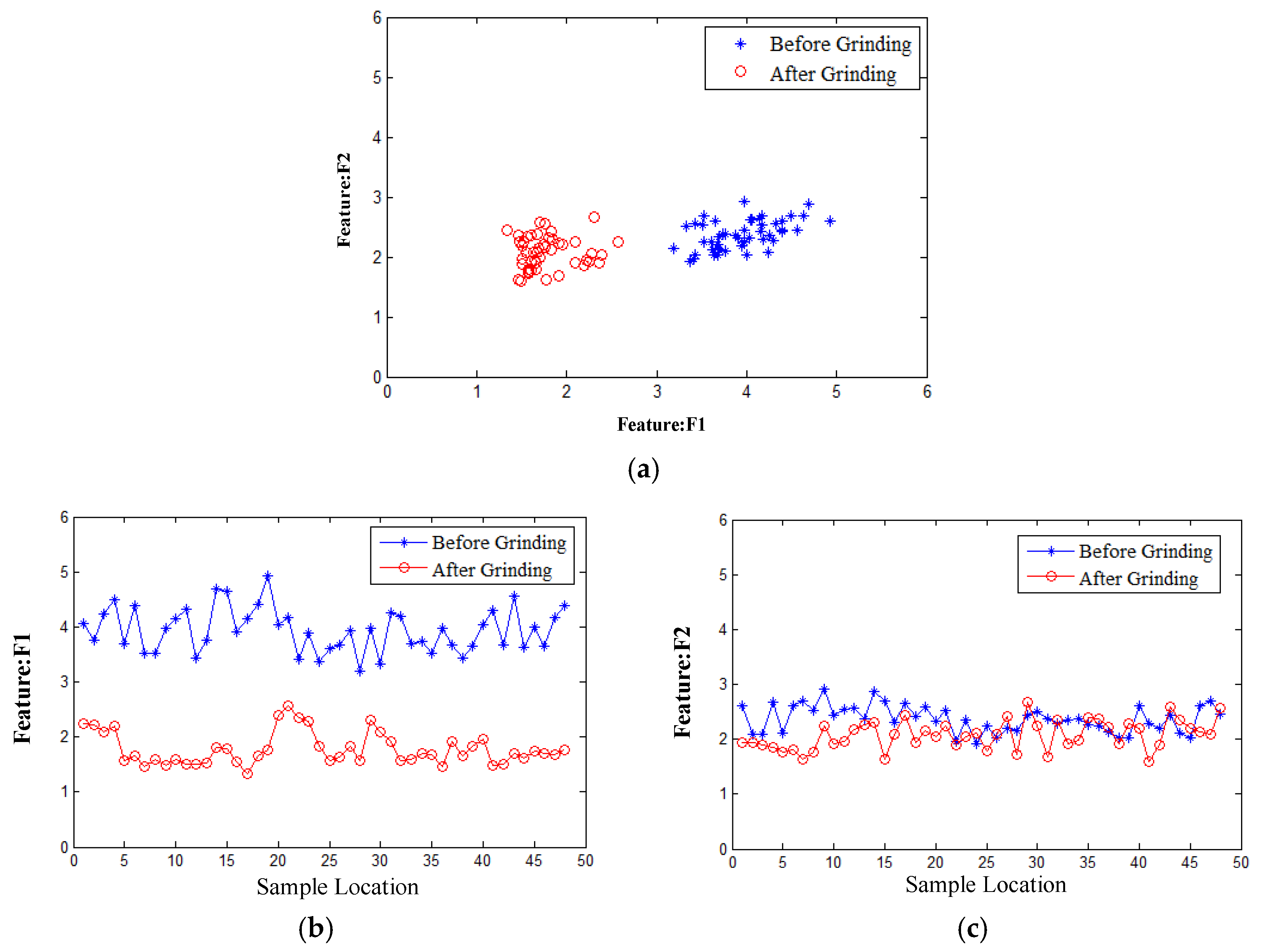
Figure 1 illustrates the manifold structure of samples before and after rail grinding in a low-dimensional space, showing good preservation of neighborhood relationships. However, in the task of state characterization, the effectiveness of feature fusion depends not only on intra-class compactness but also on inter-class separability. Figure 1a shows the projection distribution of features F1 and F2 (the distribution patterns do not represent the joint discriminative ability of the two features in 2D space, but reflect the distribution of each feature along its respective axis). Along the F1 dimension, the two states can be clearly distinguished, but the intra-class dispersion is large, indicating weak clustering. Correspondingly, in Figure 1b, the trend curves of F1 before and after grinding show noticeable differences, effectively reflecting changes in rail condition, but the curves themselves fluctuate considerably, indicating insufficient stability. In contrast, the F2 dimension exhibits good intra-class clustering, but the coordinate values of the two classes heavily overlap, reflecting poor separability. Correspondingly, Figure 1c shows the F2 trend curves before and after grinding, which fluctuate a little but almost completely overlap, indicating that while this feature is stable, it lacks the ability to characterize state changes.

In summary, clustering reflects the consistency of sample distribution under the same state and forms the basis for stable characterization of rail health. Separability reflects the degree of difference between distinct states and is a key indicator for detecting rail changes, such as grinding effects. Only by considering both clustering and separability can features maintain reliability and discriminative power in rail state recognition. To obtain indicators that preserve the internal structure of a state while remaining sensitive to rail changes, it is necessary to develop a feature fusion method that leverages the advantages of multiple features, enabling a more robust characterization of rail corrugation.

The feature distributions illustrated in this section serve as conceptual examples to motivate the manifold-based fusion perspective rather than to present actual measured data. The real vibro-acoustic measurements, data-acquisition procedures, and the computation of the six features—

• Sound-pressure RMS
• Vibration RMS
• Sound-pressure standard deviation
• Vibration standard deviation
• Sound spectral energy
• Vibration spectral energy

—are comprehensively detailed in Section 3 and Section 5.1 These later sections, based on real collected data, provide the full feature definitions and preprocessing workflow that form the experimental foundation of this study.

3. Experimental Design

3.1. Data Acquisition

Experimental data were collected from eight typical sections of a metro line in a city. These sections were selected to cover various rail corrugation conditions across different track systems, reflecting multiple typical features of corrugation.

Table 1. Experimental Information.

Section ID	Kilometer Mark	Direction	Data Acquisition & Rail Grinding Schedule
			Jan	Feb	Mar	Apr	May
S01	K10 + 200~K10 + 870	Upbound	●	★●	●	●	●
S02	K37 + 600~K38 + 200	Upbound	●★	●	●	●	●
S03	K44 + 200~K44 + 700	Upbound	●★	●	●	●	●
S04	K49 + 900~K50 + 400	Downbound	●★	●	●	●	●
S05	K40 + 800~K40 + 200	Downbound	●★	●	●	●	●
S06	K22 + 500~K23 + 000	Downbound	●	●	★●	●	●
S07	K12 + 600~K12 + 900	Upbound	●	●	●★	●	●
S08	K24 + 700~K25 + 400	Downbound	●	●	●★	●	●

Note: ● indicates data acquisition; ★ indicates rail grinding.

summarizes the experimental information. From January 2024 to May 2024, experiments were conducted once per month, resulting in a total of five experimental sessions.

Rail grinding on this metro line is performed using a dedicated rail-maintenance vehicle operated by the infrastructure department. The grinding adopts a preventive-maintenance mode, in which the rail surface is machined with multiple grinding stones to remove a thin layer of surface material, typically on the order of tenths of a millimeter. The operation targets localized corrugation segments identified by routine inspection, and the grinding length and timing follow the maintenance plan determined by the operator.

Since the grinding schedule is independent of our experiment arrangement, the grinding events (marked by ★ in Table 1) occurred naturally during the long-term monitoring period. The observed before- and after-grinding data therefore reflect the real rail-condition evolution under actual operation.

3.2. Experimental Setup

The experiments were conducted on in-service metro trains running on mainline tracks. Four sensors were installed under the train: two acoustic sensors and two vibration sensors. As shown in Figure 2, the sensors were symmetrically mounted near the axle boxes of the two wheelsets on a single bogie, with one acoustic sensor and one vibration sensor installed at each side of the axle box. This arrangement enables synchronous acquisition of vibration signals induced by rail corrugation and the sound field beneath the vehicle body.

The onboard system synchronously recorded vibration and acoustic signals at a unified sampling rate of 51.2 kHz. The acoustic sensors used were MPA201 (BSWA, Beijing, China), with a sensitivity of 50 mV/Pa and a frequency response range of 20 Hz to 20 kHz, for measuring the sound field beneath the vehicle body. The vibration sensors were JKS02J (Beijing Tangzhi Science & Technology Development Co., Ltd., Beijing, China), with a sensitivity of 40 mV/g and a frequency response range of 1 Hz to 5 kHz, mounted on the axle boxes to measure vertical accelerations induced by track excitations.

3.3. Signal Analysis

Figure 3 shows the time-domain acoustic and vibration signals for Section S01, with the horizontal axis representing the kilometer mark (km) and the vertical axes representing sound pressure (Pa) and vibration acceleration (g), respectively. It can be observed that the signal amplitudes exhibit significant differences within the 10.17–10.19 km range, while differences in other ranges are negligible. This observation aligns with the rail grinding range, as only the 10.17–10.19 km segment was subjected to grinding. Within this segment, the amplitude of the blue curve is significantly reduced compared to the red curve, indicating effective improvement in rail surface irregularity. In the unground sections, the signal amplitudes remain unchanged, maintaining similar dynamic response characteristics. Therefore, changes in rail surface condition can be directly reflected in the raw sound–vibration responses.

Short-time Fourier transform (STFT) analysis was performed on the signals in Figure 3, with the results shown in Figure 4. The horizontal axis represents kilometer marks (km), the vertical axis represents frequency (Hz), and color intensity indicates signal energy. Before grinding, both acoustic and vibration responses exhibit significant energy concentration in the 400–600 Hz frequency band, with energy peaks corresponding to the 10.17–10.19 km grinding location. After grinding, energy in this frequency band is significantly attenuated, while energy distribution in other frequency bands remains largely unchanged. This indicates that the dominant frequency of rail corrugation excitation is concentrated in the 400–600 Hz range.

4. Methodology

4.1. Theoretical Basis

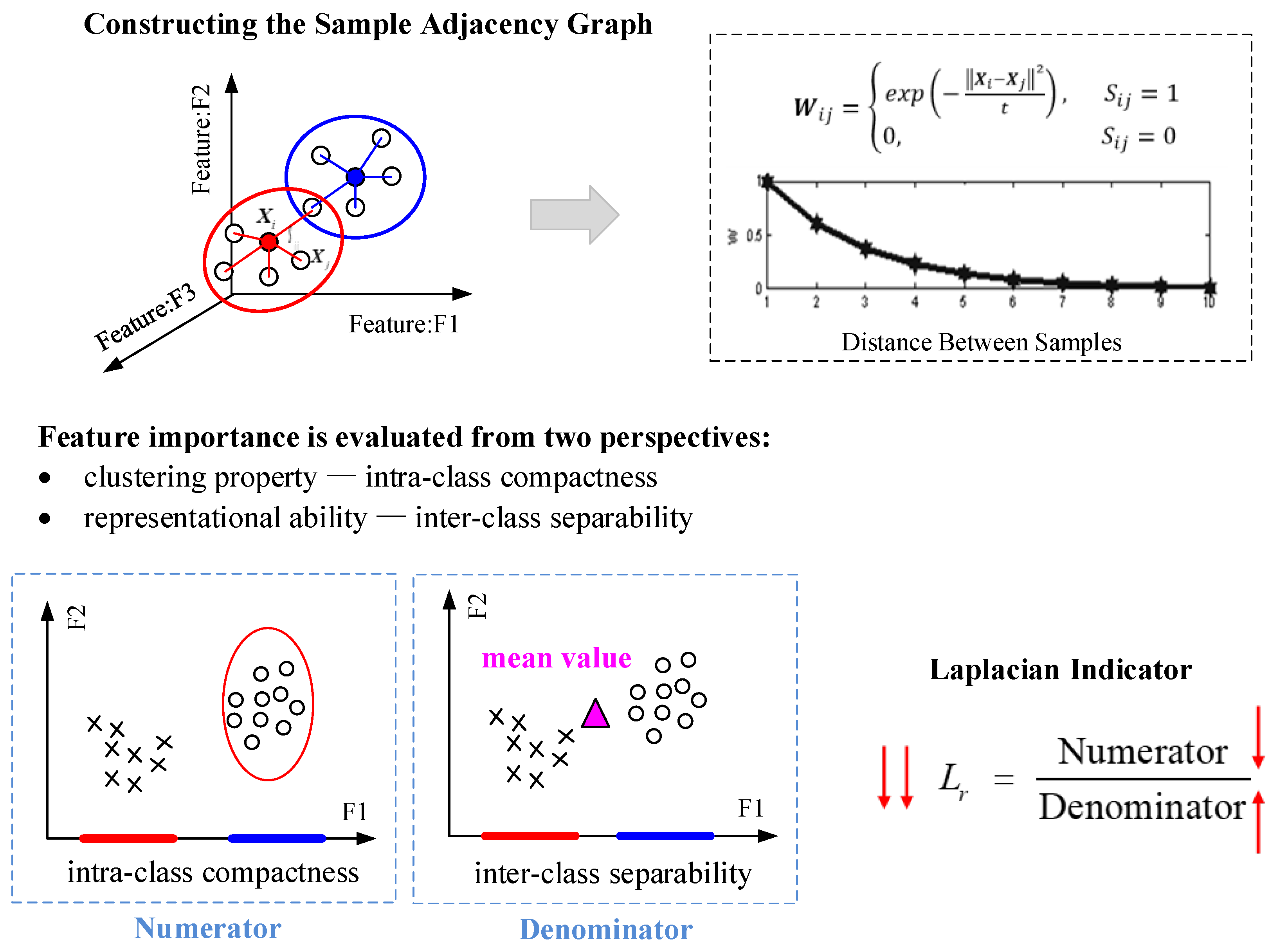
This study introduces the concept of manifold learning and extends it to construct a new feature evaluation metric: the Laplacian-based indicator L_r, as shown in Figure 5. Traditional Laplacian approaches focus on the local similarity among data points, assessing a feature’s ability to preserve these relationships, typically used to characterize intra-class compactness. However, focusing solely on intra-class compactness is insufficient to fully capture differences in rail conditions. Therefore, this study further incorporates an evaluation dimension of feature separability, comprehensively assessing feature importance from both intra-class compactness and inter-class separability perspectives.

Specifically, the proposed method measures a feature’s similarity within local neighborhoods and the overall state distribution’s dispersion to achieve a balanced assessment of clustering and separability. A smaller L_r value indicates that the feature can effectively distinguish different states while preserving local similarity. Therefore, features with smaller L_r values are more important and better reflect the evolution of rail condition.

The “manifold preservation” theory posits that points close to each other in high-dimensional space remain proximate in a low-dimensional space, and any point can be linearly represented by other points in its neighborhood, meaning that the local geometric structure of samples is preserved under dimensionality reduction.

For example, a data point in low-dimensional space can be represented as:

$$X_i={\sum }_{j=1}^k{W}_{ij}{X}_j$$

(1)

Here, X_i is expressed as a linear combination of its k nearest neighbors, and W_ij denotes the weight between X_i and its neighbors, usually related to Euclidean distance or similarity. Equation (1) reveals the local linear structure of the data: each point can be viewed as a linear combination of its neighbors, forming a locally linear approximation of the manifold.

Based on Equation (1), a kernel function is applied to map the low-dimensional points into a high-dimensional space. Let the kernel function be (⋅), then the linear relationship in high-dimensional space can be expressed as:

$$\mathrm{\varnothing }\left(X_i\right)={\sum }_{j=1}^k{W}_{ij}\mathrm{\varnothing }\left(X_j\right)$$

(2)

Equation (2) indicates that in the high-dimensional feature space after nonlinear mapping, the neighborhood relationships among data points should still be preserved. The Laplacian approach quantifies a feature’s ability to maintain local structure by constructing adjacency relationships among samples and defining a weight matrix.

4.2. Construction of Data Adjacency Graph

To characterize the local manifold structure of the data, a data adjacency graph $\mathcal{G}=\left(\mathcal{V},\mathcal{E}\right)$ is first constructed, where the vertex set $\mathcal{V}=\left\{X_1,X_2,\cdots ,X_n\right\}$, and the edge set $\mathcal{E}\subseteq \mathcal{V}\times \mathcal{V}$. The Euclidean distance between each data point and all other points is calculated. If X_j is one of the k nearest neighbors of X_i, an edge exists between X_i and X_j in the adjacency graph $\mathcal{G}$, and S_ij = 1; otherwise, if X_j is not a neighbor of X_i, then S_ij = 0.

The adjacency matrix S is defined as:

$$S_{ij}=\left\{\begin{array}{c}1,\hspace{1em}\hspace{1em}\hspace{1em}\hspace{1em}\mathrm{i}\mathrm{f} X_j\in {\mathcal{N}}_k\left(X_i\right) \mathrm{o}\mathrm{r} X_i\in {\mathcal{N}}_k\left(X_j\right)\\ 0,\hspace{1em}\hspace{1em}\hspace{1em}\hspace{1em}\mathrm{o}\mathrm{t}\mathrm{h}\mathrm{e}\mathrm{r}\mathrm{w}\mathrm{i}\mathrm{s}\mathrm{e}\hfill \end{array}\right.$$

(3)

where ${\mathcal{N}}_k\left(X_i\right)$ denotes the k-nearest neighbor set of X_i. This adjacency graph captures the neighborhood relationships between data points in the dataset. Once adjacency is established, a weight is assigned to each edge to reflect the similarity between neighboring data points.

When S_ij = 1, the edge weight is determined using a heat kernel function. The scale parameter (a constant) controls the decay of similarity. The weight W_ij is an exponentially decaying function that represents the closeness between points: the closer two points are, the larger the value of W_ij, which ranges from 0 < W_ij ≤ 1. When S_ij = 0, the weight W_ij = 0.

$$W_{ij}=\left\{\begin{array}{c}exp\left(-{\displaystyle \frac{{‖X_i-X_j‖}^2}{t}}\right),\hspace{1em}{S}_{ij}=1\\ 0, \hspace{1em}\hspace{1em}\hspace{1em}\hspace{1em}\hspace{1em}\hspace{1em}{S}_{ij}=0\hfill \end{array}\right.$$

(4)

The adjacency weight between two points acts as a penalty factor, assigning greater weight to points that are closer and smaller weight to points that are farther apart.

4.3. Determination of Feature Evaluation Indicator

Based on the established adjacency graph, the Laplacian-based indicator L_r is defined for each feature to achieve a balanced assessment of clustering and separability:

$$L_r={\displaystyle \frac{{\sum }_{i,j}{\left(f_{ri}-f_{rj}\right)}^2{W}_{ij}}{Var\left(f_r\right)}}$$

(5)

where f_ri denotes the r-th feature value of the i-th sample, f_rj denotes the r-th feature value of the j-th sample, and Var(fr) represents the global variance of the r-th feature f_r. A larger variance indicates stronger separability among feature values.

Equation (5) embodies the concept of “local clustering–global separability”: a small numerator indicates strong local clustering of the feature within neighborhoods, while a large denominator indicates a dispersed global distribution, reflecting good separability. A smaller L_r value implies that the feature performs better in maintaining local consistency while distinguishing global states, and is therefore more representative of the underlying data structure.

4.4. Sound–Vibration Feature Weighted Fusion

In this study, six basic acoustic and vibration features are extracted from sound–vibration samples (see Section 5.2 for details). The Laplacian indicator L_r of each feature is calculated according to Equation (5), and its reciprocal is used as the feature weighting coefficient:

$$A_r=1/L_r$$

(6)

where A_r represents the weighting coefficient of the r-th feature. Based on these coefficients, the sound–vibration fusion indicator is defined as:

$$LWVAF(i)={\sum }_{r=1}^R{A}_r{f}_{ri}$$

(7)

where LWVAF(i) denotes the LWVAF value of the i-th sample, and R is the total number of features. Equation (7) achieves weighted fusion under the manifold-preserving constraint, ensuring that the fused feature both reflects the continuous evolution of rail conditions and maintains good discriminative ability.

4.5. Method Workflow and Implementation

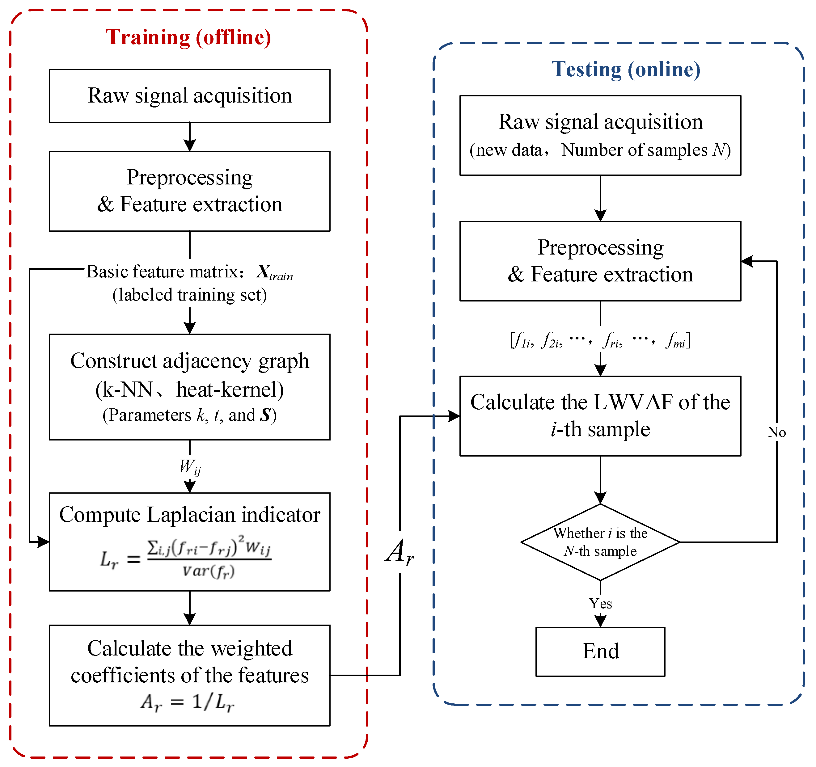
To illustrate the overall framework of the proposed method, Figure 6 presents the workflow of the sound–vibration fusion approach based on Laplacian manifold learning, which constitutes the implementation process of the sound–vibration fusion indicator LWVAF.

To ensure that the choice of neighborhood size k and kernel scale t does not bias the Laplacian-based LWVAF computation, we performed a full sensitivity analysis covering k ∈ {5, 8, 10, 12, 15, 20} and t ∈ {0.2, 0.5, 1.0, 2.0}σ². As detailed in Appendix A, both the between-section standard deviation of LWVAF and the mean reduction rate after grinding exhibit extremely small numerical variations across the k × t grid. For over 90% of the parameter combinations, the relative deviation from the baseline setting (k = 8, t = 0.5σ²) stays within ±2%. This confirms that LWVAF is robust with respect to graph-construction hyperparameters, and validates the use of the baseline setting in all experiments of this study.

5. Results Analysis and Discussion

5.1. Selection of Basic Features

Feature extraction is a key step to mine state information from raw acoustic and vibration signals. Since rail corrugation affects both the structural vibration of wheel–rail contact and acoustic radiation, six basic features are extracted separately from the acoustic and vibration signals to describe rail conditions across different physical dimensions. These six features include: root mean square (RMS) of sound pressure, RMS of vibration, standard deviation of sound pressure, standard deviation of vibration, spectral energy of sound pressure, and spectral energy of vibration.

Let the raw acoustic signal be (t) and the vibration signal be (t). The signals are first processed by band-pass filtering, with a passband of 20–20 kHz for acoustic signals and 1–5 kHz for vibration signals. The continuous acoustic and vibration signals are then sampled at 51.2 kHz and segmented using a 1 s time window. Each window is considered as an independent data sample. After discrete sampling, the acoustic and vibration data are represented as p = [p(1), p(2), …, p(k), …,p(K)]^T, a = [a(1), a(2), …, a(k), …, a(K)]^T, where K is the sample length of each data window.

The six basic features are defined as follows:

• Root Mean Square (RMS), measures the overall energy level of the signal, defined as:

$$R=\sqrt{{\displaystyle \frac{1}{K}}{\sum }_{k=1}^K{x}^2\left(k\right)}$$

(8)

where x(k) represents either p(k) or a(k), R_p denotes the RMS of the acoustic signal, and R_a denotes the RMS of the vibration signal. This metric reflects the average signal energy and characterizes the overall amplitude variation induced by rail corrugation.

• Standard Deviation (SD), describes the stability and non-stationarity of the signal, defined as:

$$D=\sqrt{{\displaystyle \frac{1}{K}}{\sum }_{k=1}^K{\left[x\left(k\right)-\overline{x}\right]}^2}$$

(9)

where x(k) represents p(k) or a(k), $\overline{x}$ is the mean of x(k), D_p denotes the standard deviation of the acoustic signal, and D_a denotes the standard deviation of the vibration signal. This metric characterizes signal dispersion, reflecting the random or periodic fluctuations of rail conditions. The acoustic SD represents the variations in the sound field, while the vibration SD reflects the fluctuation of the track structure response.

• Spectral Energy (SE), analyzes energy distribution within the dominant frequency band of rail corrugation, defined as:

$$E={\sum }_{f=f_1}^{f_2}{\left|X\left(f\right)\right|}^2$$

(10)

where X(f) is the Fourier spectrum of x(k), and f corresponds to the dominant frequency range of corrugation. Based on the analysis in Section 5.1, the range is 400–600 Hz. E_p denotes the spectral energy of the acoustic signal, and E_a denotes that of the vibration signal. Spectral energy reflects the concentration of energy in the corrugation frequency band, which is an important indicator for characterizing the strength of rail surface excitation.

The six extracted features form the feature vector for the i-th sample F_i= [R_p, R_a, D_p, D_a, E_p, E_a], and the feature matrix for all samples is F = [F₁, F₂, …, F_I]^T, where I is the total number of samples. The first four features are general indicators based on signal energy and variability, not specifically designed for corrugation, and they reflect overall signal intensity and fluctuation in the time domain, forming the basis for studying the internal manifold structure of the data. The last two features are selected based on the physical mechanism of rail corrugation. Since rail corrugation exhibits a distinct dominant frequency range and measured results show a significant energy decrease after grinding, using the energy in this frequency band as a feature effectively enhances the model’s sensitivity to rail condition changes.

5.2. Feature Weight Analysis

Although five experimental sessions were conducted, only the two sets of data corresponding to the rail conditions before and after grinding for each section were selected for manifold learning analysis, as shown in

Table 2. Experimental Data Used for Manifold Learning.

Section ID	Kilometer Mark	Direction	Data Acquisition & Rail Grinding Schedule
			Jan	Feb	Mar	Apr	May
S01	K10 + 200~K10 + 870	Upbound	●	★●	●	●	●
S02	K37 + 600~K38 + 200	Upbound	●★	●	●	●	●
S03	K44 + 200~K44 + 700	Upbound	●★	●	●	●	●
S04	K49 + 900~K50 + 400	Downbound	●★	●	●	●	●
S05	K40 + 800~K40 + 200	Downbound	●★	●	●	●	●
S06	K22 + 500~K23 + 000	Downbound	●	●	★●	●	●
S07	K12 + 600~K12 + 900	Upbound	●	●	●★	●	●
S08	K24 + 700~K25 + 400	Downbound	●	●	●★	●	●

Note: ● indicates data acquisition; ★ indicates rail grinding; ■ indicates the data used for manifold learning.

. Manifold learning assumes that, to a certain extent, the proximity between samples determines their distribution in the low-dimensional space. Therefore, by selecting the data before and after rail grinding, it is possible to effectively evaluate whether the features can reflect the continuous changes in rail conditions in a targeted manner.

A total of 790 samples were selected from Table 2 to construct the feature matrix F_6×790. Based on the theoretical method in Section 3 and Equation (5), the feature evaluation results are summarized in

Table 3. Feature Evaluation Results.

Feature	Rp	Ra	Dp	Da	Ep	Ea
Lr	0.86	0.84	4.2	2.8	2.1	0.13
Importance	3	2	6	5	4	1

:

According to the feature evaluation results in Table 3, the spectral energy of vibration (E_a) has the smallest Laplacian indicator, indicating that it contributes the most to the manifold structure of the samples and is the most discriminative for states before and after grinding. From a physical perspective, this result aligns with the excitation mechanism of rail corrugation. Rail corrugation is a typical structural irregularity, primarily causing high-frequency vibration excitation through the wheel–rail contact interface. This excitation propagates along the rail and wheel structure, significantly enhancing the vibration spectrum energy within the characteristic frequency band of 400–600 Hz. After grinding, due to the reduction in rail surface irregularity, the energy in this band decreases significantly, making the vibration spectral energy the most direct and sensitive indicator of rail surface corrugation.

In contrast, the RMS of vibration (R_a) also reflects the overall structural vibration intensity, but its time-domain averaging property reduces sensitivity to local frequency band variations. The spectral energy of sound (E_p) and RMS of sound (R_p) reflect the acoustic radiation effect of corrugation, but their stability and representativeness are slightly lower than the vibration response due to the influence of vehicle structure, carbody acoustic coupling, and environmental noise.

The standard deviations of sound and vibration (D_p and D_a) mainly characterize signal fluctuation and non-stationarity, responding relatively indirectly to rail condition changes; hence, their importance in the feature weight analysis is lower.

5.3. Trend Analysis of LWVAF

According to Equation (7), the LWVAF for each month is calculated as:

$$LWVAF={\displaystyle \frac{1}{0.86}}{R}_p+{\displaystyle \frac{1}{0.84}}{R}_a+{\displaystyle \frac{1}{4.2}}{D}_p+{\displaystyle \frac{1}{2.8}}{D}_a+{\displaystyle \frac{1}{2.1}}{E}_p+{\displaystyle \frac{1}{0.13}}{E}_a$$

(11)

Figure 7 shows the LWVAF trends from January to May for the eight sections. In the figure, the temporal variations of LWVAF values for different sections can be observed. Specifically, the rise or fall of the LWVAF reflects the improvement or deterioration of rail conditions, thereby indicating the state changes before and after grinding. Analysis of the trend plots reveals several key points:

• Significant changes after rail grinding: After grinding, the LWVAF values of all eight sections show a noticeable decrease, which is consistent with expectations and indicates that the grinding treatment significantly improved the rail surface corrugation conditions.
• Different trends across sections: Some sections exhibit relatively mild LWVAF trends reflecting slower rail degradation (e.g., S03, S04, S05), while other sections show more pronounced LWVAF variations indicating more significant rail condition changes (e.g., S01, S02, S06, S07, S08).

The LWVAF trend changes shown in Figure 7 not only reflect the temporal evolution of rail conditions but also validate the effectiveness of the Laplacian manifold learning–based feature fusion in characterizing rail corrugation. In particular, after corrugation maintenance, observing the LWVAF changes for each section allows one to relate the corrugation evolution to grinding operations, providing an important basis for dynamic monitoring and assessment of rail conditions.

5.4. Comparative Analysis

To further verify the advantage of the vibro-acoustic fusion indicator LWVAF over single acoustic or vibration indicators in rail condition characterization, this section presents both trend visualization and quantitative comparison of the three types of indicators.

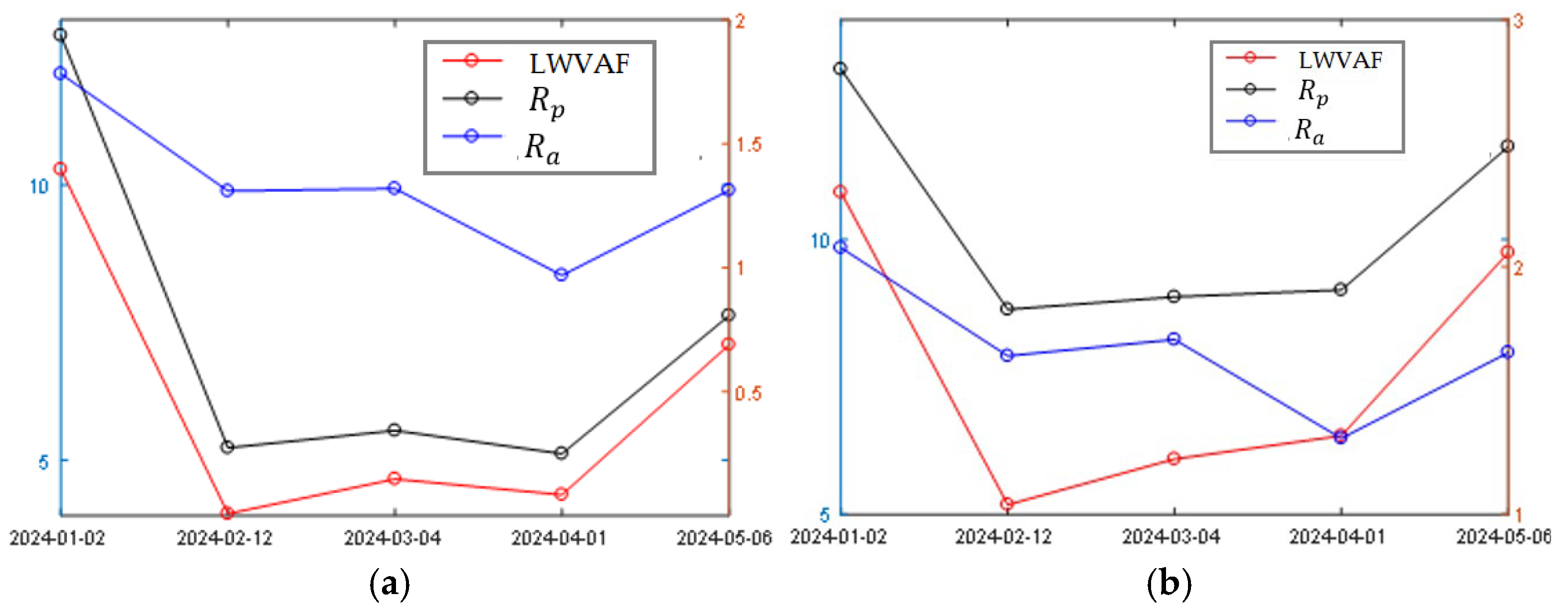
First, from the perspective of trend changes, Figure 8 shows the variations of the RMS of sound pressure, RMS of vibration, and the LWVAF for the typical Section S01 before and after rail grinding. It can be clearly observed that both the sound and vibration RMS indicators decrease to some extent after grinding, but their changes differ; in contrast, the LWVAF shows a more pronounced downward trend with smaller fluctuations.

To quantitatively compare the sensitivity of each indicator to rail condition changes, the indicator change rate is defined as:

$$\Delta r={\displaystyle \frac{{ID}_{before}-{ID}_{after}}{{ID}_{before}}}$$

(12)

where ID_before and ID_after denote the indicator values before and after grinding, respectively. A negative Δr indicates that the indicator value decreases after grinding, reflecting improvement in the rail surface condition. The larger the absolute value of Δr, the higher the indicator’s sensitivity to rail condition changes and, therefore, its characterization capability. Conversely, a smaller absolute Δr indicates lower sensitivity and weaker representation of rail condition changes.

From

Table 4. Quantitative Comparison of Trend Changes for Each Indicator.

Section ID		LWVAF Change Rate $\mathbf{\Delta }\mathit{r}$	Rp Change Rate $\mathbf{\Delta }\mathit{r}$	Ra Change Rate $\mathbf{\Delta }\mathit{r}$
S01	Left Rail	−60.81%	−58.89%	−26.53%
	Right Rail	−52.30%	−33.35%	−21.04%
S02	Left Rail	−55.66%	−48.75%	−13.77%
	Right Rail	−55.41%	−22.47%	−0.79%
S03	Left Rail	−67.37%	−59.01%	−29.94%
	Right Rail	−71.51%	−19.82%	−25.92%
S04	Left Rail	−53.21%	−28.04%	−9.62%
	Right Rail	−62.48%	−38.31%	−16.95%
S05	Left Rail	−62.58%	−58.17%	−52.46%
	Right Rail	−71.82%	−62.52%	−60.87%
S06	Left Rail	−50.67%	−53.37%	−69.54%
	Right Rail	−55.78%	−57.58%	−71.86%
S07	Left Rail	−52.90%	−42.25%	−61.59%
	Right Rail	−61.42%	−34.35%	−73.66%
S08	Left Rail	−64.73%	−54.31%	−56.58%
	Right Rail	−66.99%	−58.02%	−55.52%

, it can be observed that all three types of indicators across the sections show negative changes after grinding, indicating that the rail grinding operation generally reduces the signal energy features. Among them, the change rate of the vibration RMS indicator is relatively unstable, ranging from a minimum of 0.79% to a maximum of 73.6%. The sound RMS indicator is comparatively more stable than vibration, but in some sections the absolute change rate is relatively small; for example, the right rail of S03 shows a change rate of 19.8%, failing to exhibit a pronounced variation. In contrast, the absolute change rates of the LWVAF indicator exceed 50% across all sections, significantly higher than those of the individual sound or vibration indicators, demonstrating that the fused feature is more sensitive in capturing changes in rail conditions.

Its superior performance essentially arises from two key reasons. First, acoustic signals represent the radiated response of rail corrugation excitation in the air medium, while vibration signals directly reflect the structural response of the wheel–rail system and are therefore more sensitive to track surface irregularities. The LWVAF indicator integrates energy-related features from both acoustic and vibration domains, capturing complementary information from the two physical channels. Second, the fusion process leverages manifold learning theory to exploit the intrinsic geometric relationships within the data. Through data-driven weight learning, feature dimensions that are strongly correlated with track-state variations are amplified, whereas noise-related dimensions are suppressed. As a result, LWVAF enhances state-discrimination capability while preserving the intrinsic consistency of the samples.

5.5. Feasibility of Incremental or Adaptive Manifold Updating

The graph used in this study is constructed by k-nearest neighbors and heat-kernel weights, both of which are inherently local operators. For a newly acquired sample, only its own neighborhood relations—and the relations of a small set of points that include it in their kNN list—need to be updated. The rest of the graph remains unchanged. This locality property implies that the underlying neighborhood graph can be maintained in an incremental manner without rebuilding the entire structure.

Since the LWVAF indicator depends only on local feature differences weighted by the current graph structure, its value can be updated by refreshing the local neighborhoods and their associated weights. No global recomputation of all pairwise relations is required. This property makes the LWVAF framework naturally compatible with adaptive or streaming data settings.

Depending on the continuity and rate of incoming data, several practical updating strategies are feasible:

• Incremental updates: update graph and LWVAF only when new samples arrive.
• Mini-batch updates: process data in short windows (e.g., 5–10 min).

These schemes require minimal computational overhead because only local modifications are made.

While the locality of the graph structure enables incremental updates, several engineering considerations remain:

• Drift in long-term data distributions may require occasional reinitialization of the neighborhood graph.
• Extreme outlier samples may distort local neighborhoods and should be detected prior to updating.
• Computation on edge devices may restrict update frequency, requiring simplified neighborhood search.

Overall, the graph structure and LWVAF formulation used in this study possess natural mathematical and computational properties that make them suitable for incremental or adaptive manifold updating in long-term monitoring systems.

6. Conclusions

A manifold-learning-based acoustic–vibration fusion method for track-state representation was developed. By applying Laplacian manifold analysis, the adjacency relationships among acoustic–vibration samples were constructed, enabling the characterization of their distribution in a low-dimensional manifold space. From the perspective of feature-space locality, the method reveals the latent clustering properties of track-state features. This framework provides theoretical support for multimodal feature fusion, allowing acoustic and vibration information to be represented within a unified manifold space.

An acoustic–vibration fusion index, LWVAF, based on Laplacian weighting was proposed. Six fundamental features—acoustic RMS, vibration RMS, acoustic standard deviation, vibration standard deviation, acoustic spectral energy, and vibration spectral energy—were adaptively weighted through the Laplacian weighting mechanism to form the fusion index LWVAF. The results demonstrate that Laplacian weights effectively reflect the importance of each feature within the manifold structure, enabling adaptive feature-level fusion and overcoming the limitations of conventional subjective weighting approaches.

The superiority of the fusion index in track-state representation was validated. Trend analysis and change-rate evaluation across eight experimental sections show that LWVAF exhibits more pronounced trend variations and consistently larger absolute change rates before and after rail grinding. Compared with using acoustic or vibration indicators alone, LWVAF is more sensitive and stable in capturing changes in track condition. This confirms the robustness and enhanced representational capability of the proposed fusion method.

This study establishes a quantitative evaluation method for track condition characterization. By constructing a quantitative mapping between acoustic–vibration features and track states based on the LWVAF index, the proposed approach provides a measurable basis for assessing rail grinding effectiveness. The method exhibits strong robustness and engineering applicability under diverse operating conditions, and it holds promising potential for integration into onboard real-time diagnostic systems. It can also be extended to long-term track health monitoring, offering particular advantages in scenarios with limited prior knowledge. Leveraging its unified acoustic–vibration characterization framework and adaptive fusion capability, the method can further be applied to localized track defect detection. In addition to urban rail systems, the approach is equally applicable to more complex railway networks such as high-speed and heavy-haul railways.