Application Exploration of Flow Field Prediction in Free Jet Tests Based on Proper Orthogonal Decomposition Method

Abstract

This study focuses on the demand for rapid prediction of the flow field of aero-engine inlet free jet tests and explores the application of radial basis function interpolation (RBF) and backpropagation neural network (BPNN) methods. The proper orthogonal decomposition (POD) method was used for model order reduction of the full-order flow field results from numerical simulations. Two rapid prediction methods, namely POD-RBF and POD-BPNN, were constructed by utilizing radial basis function interpolation and a backpropagation neural network. These methods successfully achieved rapid prediction of the test flow field under different Mach numbers and angles of attack. To verify the accuracy of the numerical simulation and rapid prediction methods, a free jet test of the jet inlet was conducted under the same conditions. The test results show good agreement with both the CFD calculation results and the rapid prediction results. The research results show that the ninth-order mode can accurately reconstruct the flow field structure with a reconstruction error of 1.83%. Both methods can quickly and accurately predict the flow field under different conditions, and the prediction results are in good agreement with the numerical simulation results. Generally speaking, the prediction error of the POD-BPNN method is smaller than that of the POD-RBF method.

1. Introduction

The free jet test mainly conducts a joint test on the inlet-engine [1]. It requires placing the air inlet-engine in the free jet flow and demands that the inlet reference plane (IRP) in front of the inlet entrance has similarity to the real working environment [2,3,4]. The free jet Mach number, flow angle, outlet area of the free jet nozzle, and relative position between the nozzle outlet and the test object, which are associated with this requirement, are all factors affecting the similarity of this section [5].

To ensure the success of the test on the first attempt, it is necessary to conduct flow prediction under test conditions and verification of test similarity before the test is carried out. However, for a long time, there has been an irreconcilable contradiction between calculation speed and calculation accuracy. Numerical simulation has high accuracy and can predict high-dimensional flow field structures, but it is slow and thus difficult to use for rapid prediction; simple zero-dimensional or one-dimensional analytical models are fast in speed but low in accuracy and cannot accurately characterize the flow field quality and two-dimensional/three-dimensional distribution of key parts, such as the IRP section, in the test.

In recent years, with the development of artificial intelligence technology, intelligent algorithms have been gradually applied to flow prediction. This method boasts high accuracy, and most importantly, it can achieve second-level flow field structure prediction and output results quickly [6]. Therefore, exploration of the application of intelligent flow field prediction methods in free jet tests is necessary [7,8,9].

In terms of rapid flow field prediction, model order reduction is a type of method that reduces the system dimension, improves calculation speed, and shortens calculation time [10,11]. In the free jet tests, model order reduction can extract the main features of the system under the premise of retaining the main dynamic characteristics of computational fluid dynamics numerical simulation. Therefore, building a rapid prediction model on the basis of feature extraction through model order reduction is a very important method.

Model order reduction includes methods such as proper orthogonal decomposition (POD) [11], flow pattern learning, and autoencoder (AE) of neural networks [12,13]. Among them, although the POD method is a dimensionality reduction method based on linear theory, numerous studies have confirmed that the POD method still has good dimensionality reduction capabilities when dealing with nonlinear and complex problems such as turbulence and shock wave separation vortices in air inlets [14,15,16,17,18,19].

After model order reduction, it is necessary to build a rapid prediction model based on the main features extracted through model order reduction. At present, methods such as radial basis function (RBF) [20,21] and backpropagation neural network (BPNN) [22,23,24] have been widely applied in various prediction models. Among them, the radial basis interpolation function method has advantages such as a simple function form, fast interpolation speed, and independence from grid topology. In essence, it addresses the problem of surface fitting or approximation in high-dimensional space, and it has been widely applied in fields such as computational fluid dynamic grid processing and fluid–structure interaction [25]. However, in the field of free jet tests, there has been no publicly published literature that comprehensively adopts model order reduction and radial basis interpolation for flow prediction so far.

This paper mainly focuses on free jet inlet tests and explores a rapid prediction method for the evolution of test flow fields under different conditions based on proper orthogonal decomposition (POD) model order reduction and radial basis function interpolation. It lays a technical foundation for the digital twin of such tests.

2. Physical Model and Numerical Simulation Method

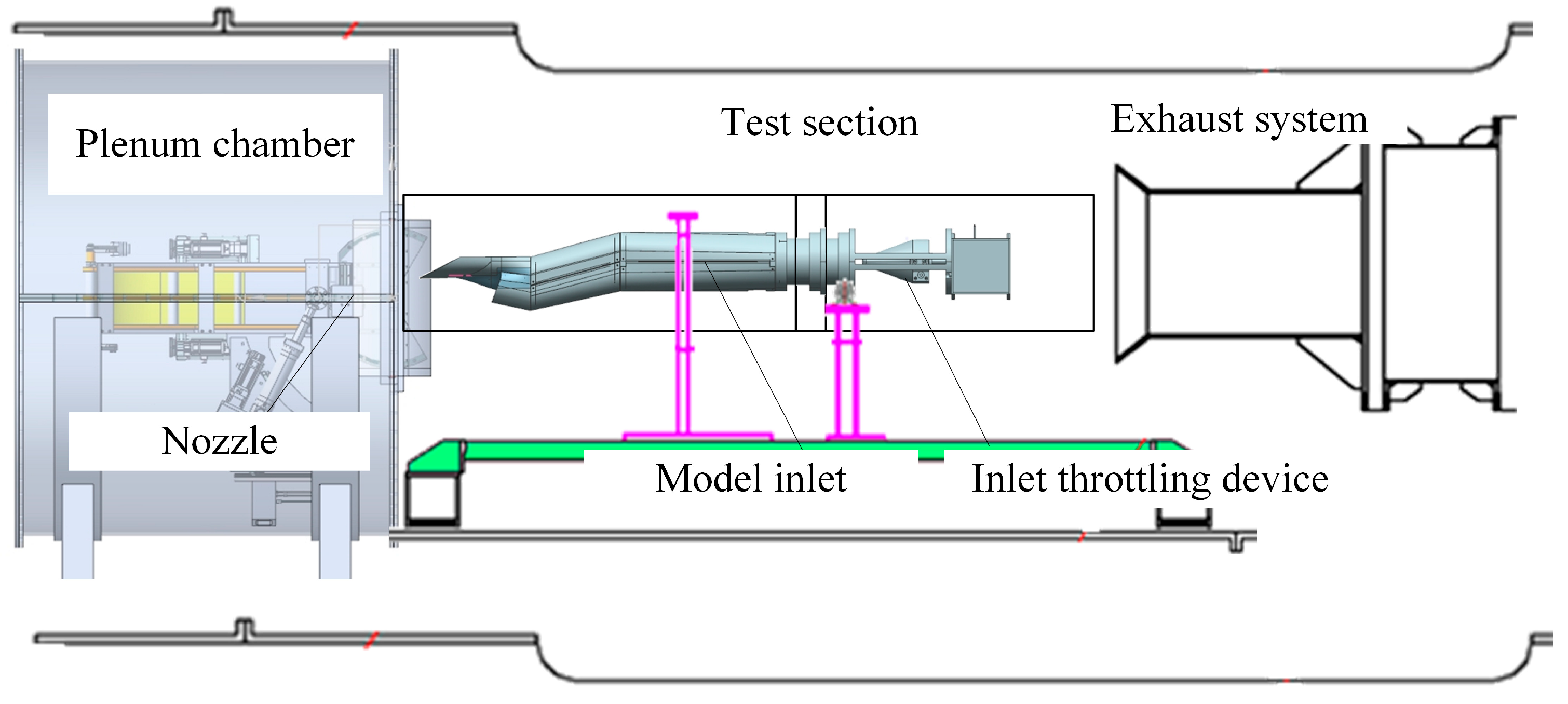
The physical model studied in this paper is shown in Figure 1. A variable Mach number nozzle is installed in the plenum chamber, enabling tests with an incoming flow Mach number ranging from 0 to 2.5. The pitch angle can be continuously adjusted within the range of −8° to 22°, and the yaw angle can be continuously adjusted within the range of −20° to 20°. A model inlet and a throttling device are installed in the test section.

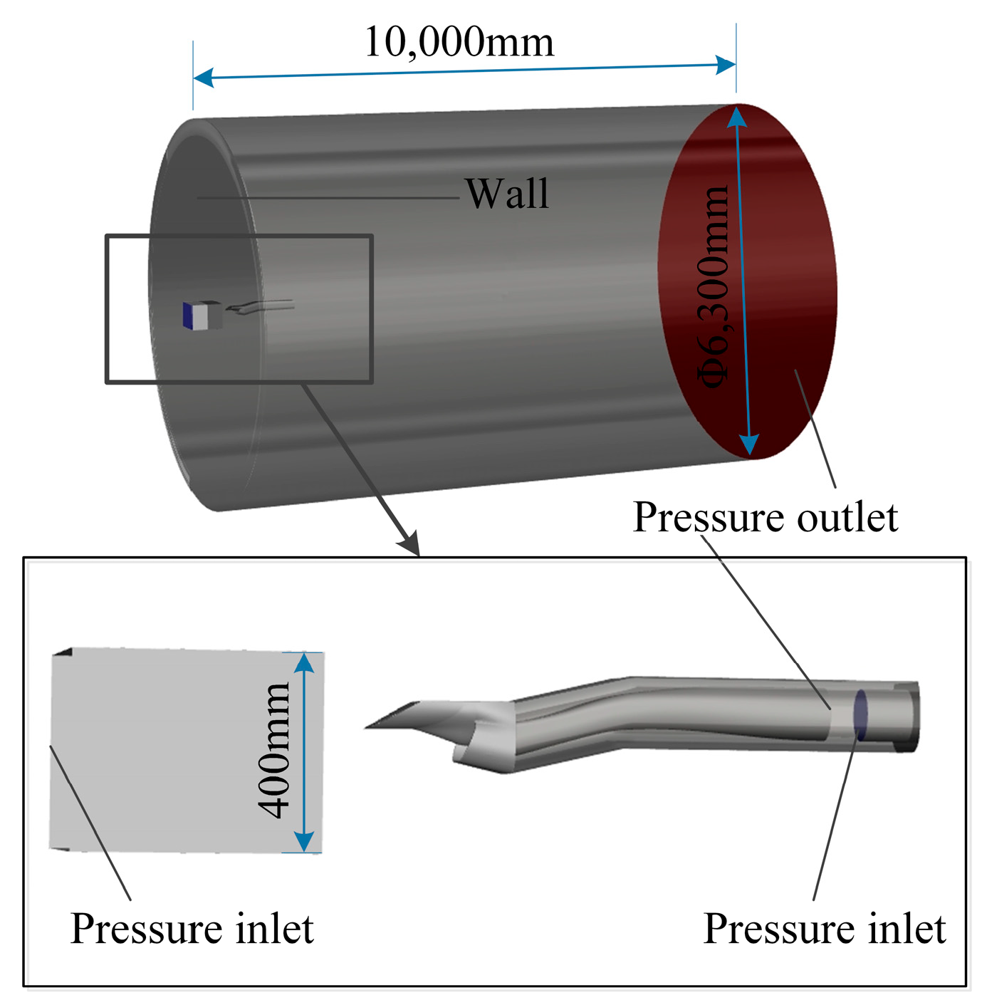
Some simplifications have been made to the simulation model established in this study. The acceleration process of the airflow in the free jet nozzle is ignored, and only the flow between the jet nozzle and the model inlet field is considered, simplifying the profile of the jet nozzle to a straight section. In general, the static pressure in the test section can fully reach the target simulated nozzle exit back pressure during the test; to reduce the computational load, the exhaust system has been omitted and the target static pressure values in the test section have been set. The exit of the inlet is set as a pressure outlet to reflect the engine’s influence on the inlet. To simulate engine exhaust, a section after the inlet is set as a pressure inlet. In the test, the method of moving throttling is adopted to simulate the back pressure of the inlet.

After the above simplifications, the computational domain of the numerical simulation is shown in Figure 2. The computational domain consists of a cylindrical test chamber and a nozzle. The cylindrical test chamber has a diameter of 6300 mm and a length of 10,000 mm, while the width and height of the nozzle’s exit cross-section are 500 mm and 400 mm, respectively. In this study, we assume a cuboid with length, width, and height of 500 mm, 500 mm, and 400 mm to represent the equipment nozzle, and half of the nozzle’s length extends out of the test chamber. The forebody-inlet duct has a length of 1182 mm, and the exit diameter of the inlet duct is 110 mm. The distance between the nozzle exit and the inlet model is 120 mm, and the free jet nozzle exit extends into the interior of the test chamber.

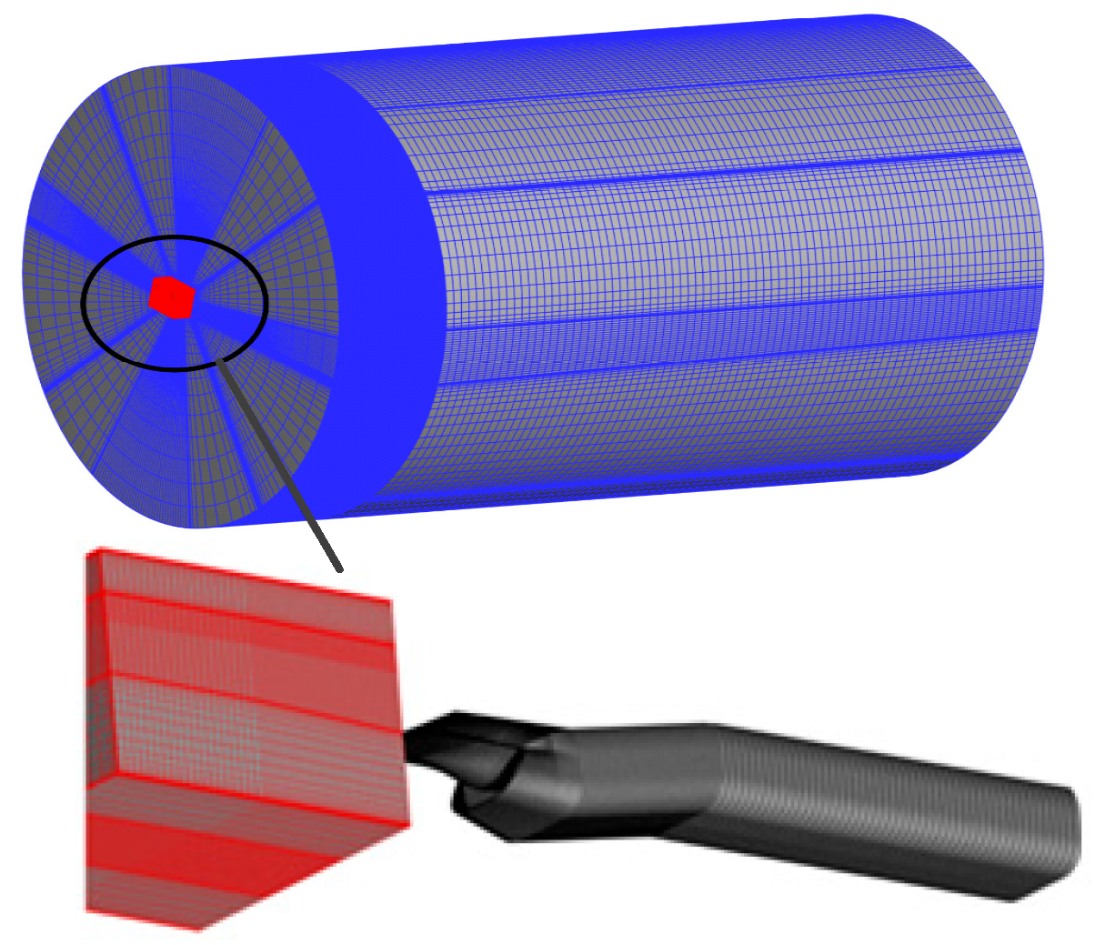
During mesh generation, mesh refinement is applied to the wall surface. The height of the first mesh layer is set to 0.003 mm so that the y+ is 0.9 as the unit Reynolds number is 8,100,000, the mesh growth rate is 1.1, and the total number of meshes is 7.1 million. In this paper, the Fluent 16.0 solver is used to solve the Reynolds-averaged conservative governing equations. Air is assumed to be an ideal gas, and unsteady effects are neglected; the flow field is assumed to be three-dimensional and steady. The Shear Stress Transport (SST) k-ω model is adopted as the turbulence model, the second-order accurate AUSM+ scheme is used for convective fluxes, and the viscous terms are obtained via the central difference scheme. The molecular viscosity coefficient is calculated using the Sutherland formula, while the turbulent viscosity coefficient is computed through the turbulence model. A convergence criterion of a five-order-of-magnitude reduction in residuals is employed.

The inlet of the jet nozzle is set as a pressure inlet boundary with the total pressure and total temperature inlet conditions specified. At a Mach number of 2.0, the altitude is 15 km, and the altitudes for other Mach numbers are determined based on the constant dynamic pressure condition. Once the altitude and Mach number are confirmed, the other inlet boundary flow field parameters can be derived, with the turbulence intensity set to 5%. The outlet of the test chamber is configured as a pressure outlet boundary, where pressure conditions simulating the flight altitude are applied. Its flow field parameters such as pressure and temperature are consistent with the boundary values of the test chamber nozzle. The outlet of the air inlet (or inlet duct) is set as a pressure outlet boundary, with pressure conditions simulating the established back pressure. In this study, the inlet exit back pressure is the same as the nozzle of test chamber. All other boundaries are defined as no-slip adiabatic walls. The specific settings are shown in Figure 3.

3. Method for Rapid Prediction of Flow Field

3.1. General Research Protocol

The overall plan of the fast flow field prediction algorithm is presented in Figure 4, and the details are as follows:

(1)

Determine the variables for flow prediction

In this paper, the free stream Mach number and angle of attack are selected as the prediction variables.

(2)

Design of experiments

An experimental design (design of experiments, DOE) is conducted for the variables to obtain a series of sample operating conditions. Based on the actual conditions of the test, this paper considers the flow field prediction of a single variable. To ensure the uniform distribution of samples, the uniform sampling method is selected.

(3)

Create data samples

This paper adopts computational fluid dynamics (CFD) methods to create data samples. The simulation results form a data sample set, namely the flow field “snapshots”.

(4)

POD decomposition

The three-dimensional flow field sample set is subjected to POD decomposition to obtain basis modes and basis coefficients, thereby achieving model order reduction, which will be described in detail in the following text.

(5)

Flow field prediction

It is assumed that the modes of the flow system under the free jet test condition to be predicted are consistent with those during model order reduction. Therefore, the focus is on developing a prediction algorithm to obtain the basis coefficients of the flow system. In this paper, two rapid prediction methods—namely the RBF interpolation method and the BP neural network—are established to predict the basis coefficients of the complex flow system in the test section, thereby realizing flow field prediction.

To reflect the degree of deviation between the predicted values and the CFD calculation results and to measure the accuracy of the prediction model, the prediction error $E_{\mathrm{r}}$ is defined based on the grid nodes as follows:

$$E_{\mathrm{r}}=\sqrt{{\displaystyle \frac{{\displaystyle \sum _{i=1}^M{({u_i}^{\mathrm{CFD}}-u_i^{\mathrm{POD}})}^2}}{{\displaystyle \sum _{i=1}^M{u}_i^{{\mathrm{CFD}}^2}}}}}$$

(1)

In the formula, $M$ is the number of grid nodes, and $u$ represents an arbitrary flow field variable.

3.2. Rapid Prediction Algorithm

3.2.1. POD Model Order Reduction Method

POD is a mathematical method for extracting system characteristics. Before model order reduction, it is necessary to obtain flow field data samples under different operating conditions and, on this basis, construct a sample matrix:

$$\mathit{u}=\left[\begin{array}{cccc}{u}_{11}& u_{12}& \cdots & u_{1N}\\ u_{21}& u_{22}& \cdots & u_{2N}\\ ⋮& ⋮& \ddots & ⋮\\ u_{M1}& u_{M2}& \cdots & u_{MN}\end{array}\right]=\left[\begin{array}{cccc}{\mathit{u}}_1& {\mathit{u}}_2& \cdots & {\mathit{u}}_N\end{array}\right],$$

(2)

where $N$ represents the number of sample operating conditions. To prevent a single singular value from being significantly larger than the others during the decomposition process, the sample matrix is processed to obtain its fluctuation matrix:

$${\mathit{u}}^{\mathit{\prime }}=[\begin{array}{cccc}{\mathit{u}}_1-\overline{\mathit{u}}& {\mathit{u}}_2-\overline{\mathit{u}}& \cdots & {\mathit{u}}_N-\overline{\mathit{u}}\end{array}].$$

(3)

In the formula, $\overline{\mathit{u}}={\displaystyle \frac{1}{N}}{\displaystyle \sum _{i=1}^N{\mathit{u}}_i}$ represents the average value of the flow field data.

The essence of the proper orthogonal decomposition (POD) method is to find a set of optimal orthogonal bases $\mathit{\Phi }$ (referred to as POD modes). This ensures that the projection of ${\mathit{u}}^{\mathit{\prime }}$ onto these orthogonal bases yields the optimal solution in the sense of least squares—specifically, the 2-norm (or L₂-norm) of the difference between the projected values and the true values is minimized:

$$\underset{\mathit{\Phi }}{\min }{\displaystyle \sum _{i=1}^N‖{\mathit{u}}_i^{\mathit{\prime }}-\mathit{\Phi }{\mathit{\Phi }}^{\mathrm{T}}{\mathit{u}}_i^{\mathit{\prime }}‖},{\mathit{\Phi }}^{\mathrm{T}}\mathit{\Phi }=\mathit{I}.$$

(4)

This minimum value can be solved using the Singular Value Decomposition (SVD) method. By mapping the flow field data ${\mathit{u}}_i^{\mathit{\prime }}$ of each operating condition onto $\mathit{\Phi }$, the corresponding basis coefficient $\mathit{a}$ is obtained.

$$\mathit{a}=[\begin{array}{cccc}{\mathit{a}}_1& {\mathit{a}}_2& \cdots & {\mathit{a}}_N\end{array}].$$

(5)

POD performs modal truncation based on the “energy” proportion [10]. By solving the eigenvalues ${\lambda }_i$ of the sample matrix and retaining the first k-order modes with a relatively high energy proportion (usually reaching approximately 99% of the “energy”), the main features of the flow field can be preserved, thereby improving computational efficiency. The “energy” of the first k-order modes is defined as

$$E(k)={\displaystyle \frac{{\displaystyle \sum _{i=1}^k{\lambda }_i}}{{\displaystyle \sum _{i=1}^N{\lambda }_i}}}.$$

(6)

In the equation, ${\lambda }_i$ represents the i-th eigenvalue of the correlation matrix $\mathit{R}={{\mathit{u}}^{\mathit{\prime }}}^{\mathrm{T}}{\mathit{u}}^{\mathit{\prime }}$, and the superscript “$T$” denotes transposition. In this way, when any i-th sample is selected, the flow field of this sample in the low-dimensional space can be described as

$${\mathit{u}}_i={\displaystyle \sum _{\mathit{j}=1}^{\mathit{k}}{a}_{ij}{\mathit{\Phi }}_j}+\overline{\mathit{u}}.$$

(7)

Thus, the order reduction in the flow field is successfully achieved, simplifying the original flow field with multiple degrees of freedom into a linear superposition of k modes for characterization. In the field of computing, computers operate extremely fast while performing addition. Therefore, in principle, POD lays a mathematical foundation for the high-speed characteristic of prediction methods.

3.2.2. Interpolation Prediction Method

Solving the basis coefficients is the key to predicting the flow field under unknown operating conditions. Interpolation is a classic mathematical calculation method, while RBF interpolation is an interpolation method that uses radial basis functions as templates and takes the Euclidean distance between unknown points and known points as the independent variable. It is widely used in various fields such as aeroelasticity, dynamic grids, and meshless methods. Using the RBF interpolation method, the basis coefficient $\mathit{a}$ can be expressed as

$${\mathit{a}}^{\mathrm{T}}=\mathit{r}\mathit{w}.$$

(8)

In the formula, $\mathit{w}$ is the weight coefficient matrix, and $\mathit{r}$ is the radial basis function value matrix.

$$r_{ij}=\phi ({‖X_i-X_j‖}_2)\hspace{1em}i,j=1,2,\cdots \cdots ,N$$

(9)

In the formula, ${‖•‖}_2$ is the Euclidean norm, $X$ is the independent variable vector, and $\phi$ is the radial basis function. Radial basis functions have various expression forms, such as the multiquadric radial basis function, the inverse quadratic radial basis function, and the Gaussian radial basis function. Among them, the Gaussian radial basis function is the most commonly used one. In the formula, $c$ is the shape parameter. In this paper, the Gaussian radial basis function interpolation method is selected for prediction, where the shape parameter c is set as 0.3.

$$\phi ({‖X_i-X_j‖}_2)=e^{-c^2{‖X_i-X_j‖}_2^2}$$

(10)

3.2.3. BP Neural Network

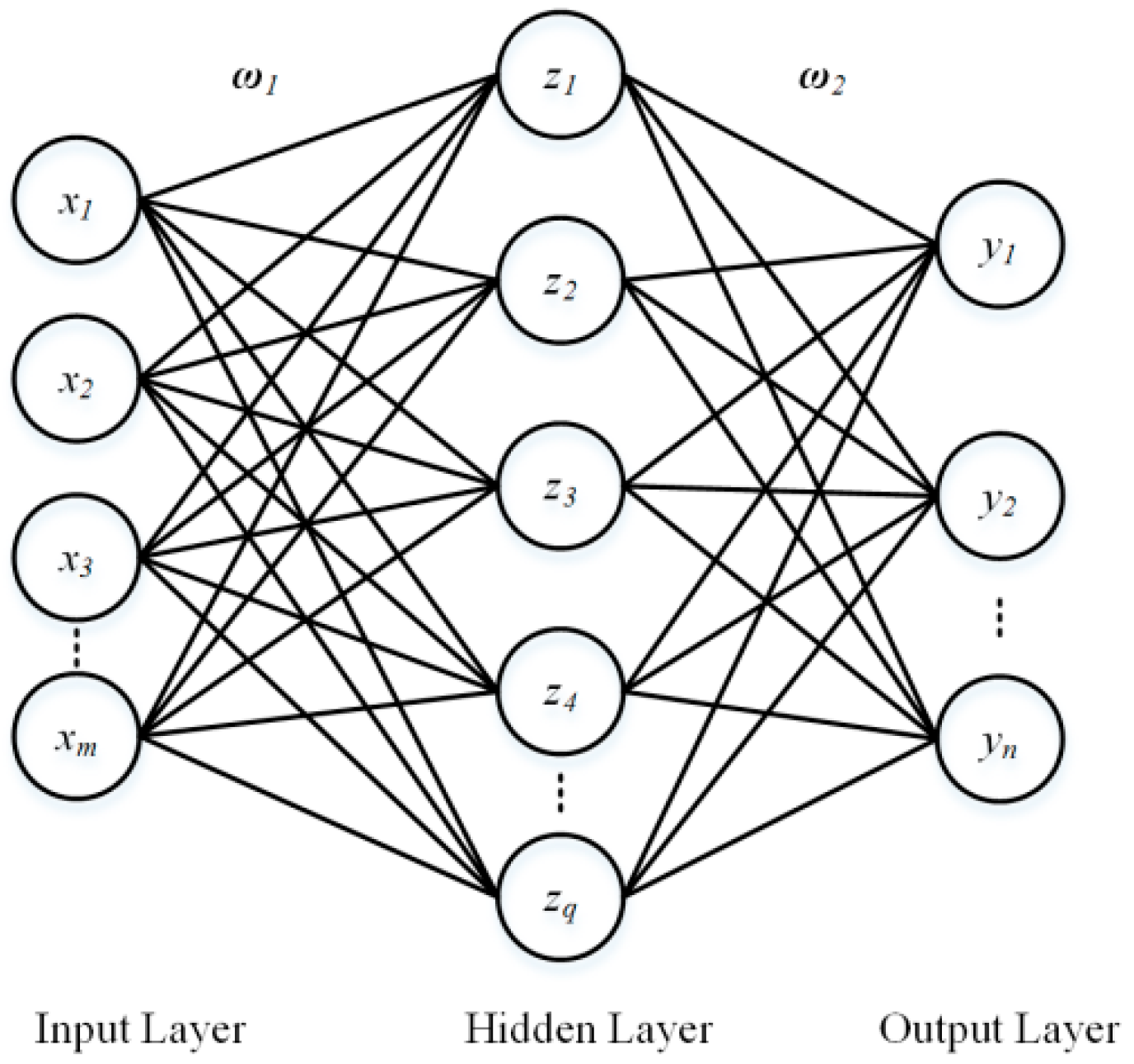
The backpropagation (BP) neural network is a feed-forward multi-layer network based on the error backpropagation algorithm, and it is one of the most widely used neural network models. In this paper, the BP neural network is adopted to establish the mapping relationship between the input parameters of sample operating conditions and their corresponding basis coefficients. A basic BP network consists of three layers: the input layer, the hidden layer, and the output layer. It processes the weighted input through an activation function to obtain the output.

This paper selects a single hidden layer network as the prediction model, as shown in Figure 5. This network establishes a mapping relationship from m-dimensional input to n-dimensional output. In this network $x$ represents the input layer parameters, i.e., the input parameters of sample operating conditions; y denotes the output layer results, i.e., the corresponding basis coefficients; $z$ stands for the hidden layer parameters; and $\omega$ is the weight matrix.

The activation function uses the classic tanh function:

$$\tanh x={\displaystyle \frac{e^x-e^{-x}}{e^x+e^{-x}}}.$$

(11)

The Levenberg–Marquardt (LM) algorithm is adopted for the BP neural network in this paper, which avoids the defects of the traditional BP neural network algorithm, such as slow iteration speed and a strong tendency to fall into local minima. The LM algorithm is an improved form of the Gauss–Newton method, possessing both the local characteristics of the Gauss–Newton method and the global characteristics of the gradient method. The principle of the LM algorithm is as follows: assuming that $\mathit{W}(\mathit{k})$ is the network weight vector of the $\mathit{k}$-th iteration, $\mathit{W}(\mathit{k}+1)$ can be obtained by the following formula,

$$\mathit{W}(\mathit{k}+1)=\mathit{W}(\mathit{k})+\Delta \mathit{W}(\mathit{k}).$$

(12)

Regarding the Levenberg–Marquardt (LM) algorithm,

$$\Delta \mathit{W}=-{\left[{\mathit{J}}^{\mathrm{T}}(\mathit{W})\mathit{J}(\mathit{W})+\mathit{\mu }\mathit{I}\right]}^{-1}\mathit{J}(\mathit{W})\mathit{e}(\mathit{W}).$$

(13)

In the equation, $\mathit{\mu }>0$ is a constant, I is the identity matrix, and $\mathit{J}(\mathit{W})$ is the Jacobian matrix. The matrix $\mathit{e}(\mathit{W})$ is expressed as follows:

$$\mathit{e}(\mathit{W})={\left[{\mathit{e}}_1(\mathit{W}),{\mathit{e}}_2(\mathit{W}),\dots ,{\mathit{e}}_{\mathit{N}}(\mathit{W})\right]}^{\mathrm{T}}.$$

(14)

Any column vector of the matrix is

$${\mathit{e}}_{\mathit{i}}\left(\mathit{W}\right)={\mathit{u}}_{\mathit{i}}-{\mathit{v}}_{\mathit{i}}.$$

(15)

In the equation, ${\mathit{u}}_{\mathit{i}}$, ${\mathit{v}}_{\mathit{i}}$ are the errors between the expected output and the actual output. The mean squared error (MSE) is used as the loss function in the training process, which is expressed as follows:

$$\mathrm{MSE}={\displaystyle \frac{1}{\mathit{N}}}{\displaystyle \sum _{\mathit{i}=1}^N(\mathit{y}-\widehat{\mathit{y}}}{)}^2.$$

(16)

In the formula, $\mathit{y}$ represents the true value, and $\widehat{\mathit{y}}$ denotes the predicted value. In this research, the neural network architecture consists of one hidden layer with 15 neurons predicting the flow field. The training process employs the following stopping criteria: a maximum number of iterations of 1000, a mean squared error below 1 × 10⁻⁷, and an error gradient magnitude smaller than 1 × 10⁻⁷.

3.3. Regional Difference Method for Motion Boundaries

Different angles of attack are simulated by rotating the free jet nozzle, which makes the boundaries of the flow prediction region dynamically changing. The traditional POD method is difficult to use to solve such problems. To this end, this paper develops a method to interpolate and project the flow fields in the region in front of the inlet under different nozzle rotation angles onto an invariant background grid. The interpolation method is implemented using the radial basis function (RBF) interpolation:

$$\begin{array}{l}{\mathit{y}}_j={\displaystyle \sum _{\mathit{i}=1}^N{\lambda }_i\phi }({‖{\mathit{X}}_{\mathit{i}}-{\mathit{X}}_{\mathit{j}}‖}_2).\end{array}$$

(17)

The coefficients in Equation (17) are obtained by solving a system of $N$ equations, where $i$ denotes the index of any arbitrary point in the grid under different angles of attack, and j denotes the corresponding index in the fixed background grid.

3.4. Sample Generation Method

The sample data in this paper are mainly derived from the numerical calculation results of flow fields obtained from tests under different flight Mach numbers and different flight angles of attack. The variation ranges of the Mach numbers and angles of attack are presented in

Table 1. The variation ranges of the parameters.

Variable	Lower Limit	Upper Limit	Sampling Interval
Mach number	0.4	2.5	0.1
Angle of attack	−10°	10°	1°

; the Mach number ranges from 0.4 to 2.5, the angle of attack ranges from −10° to +10°, and the simulated altitude is 15 km. Among these parameters, the sampling interval calculated based on the Mach number is 0.1, and the sampling interval for the angle of attack is 1.

When the Mach number is used as the predictive variable, the angle of attack is 0°; when the angle of attack is used as the predictive variable, the Mach number is 2.0. In principle, the multi-variable prediction is similar to the single-variable prediction, and it will not be repeated in this paper.

4. Test Verification of Simulation and Prediction Results

The test scenario is shown in Figure 1 in the above text. The cross-sectional dimensions of the free jet nozzle exit are 400 mm (height) × 500 mm (width). The test incoming flow Mach number is continuously variable within the range of 0–2.5, and the model inlet used in the test is consistent with the model inlet used in the aforementioned flow prediction.

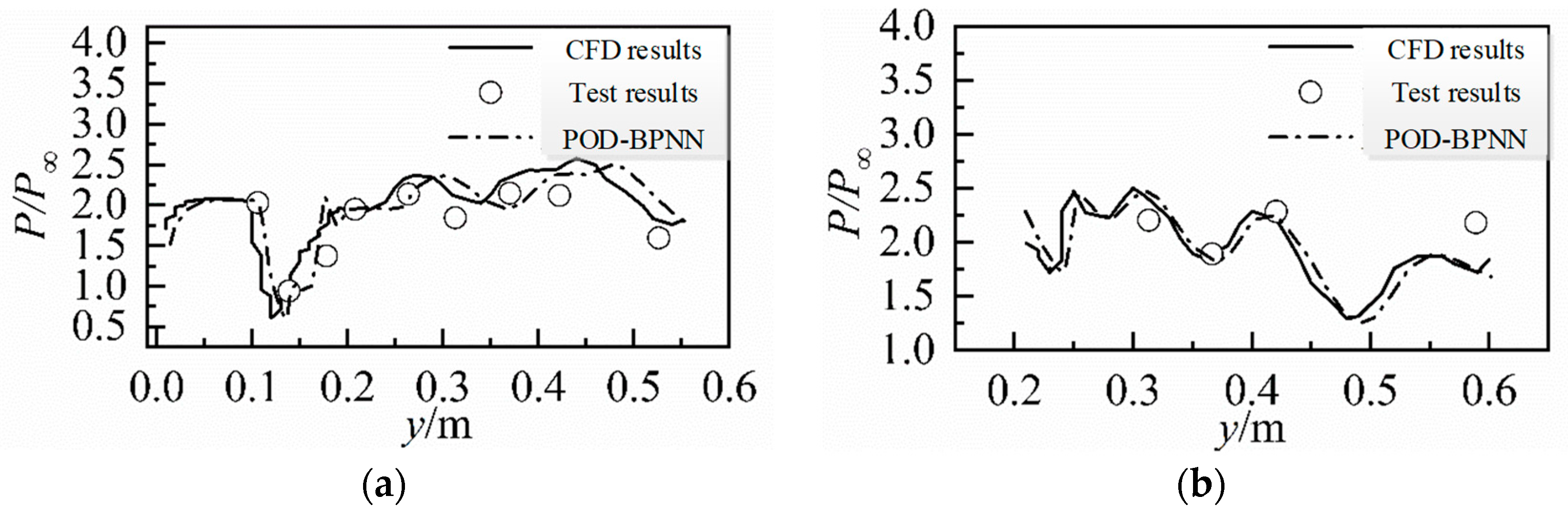
The test was conducted under the conditions of a simulated flight altitude of 15 km, a flight Mach number (Ma) of 2.0, and an angle of attack of 0°, with all tests performed in the flow-through state of the inlet. The comparison between the test results of the static pressure along the inlet wall, the CFD calculation results, and the POD-BPNN prediction results is presented in Figure 6. The predicted pressure results along the upper and lower walls of the inlet show good agreement with both the CFD calculation results and the test data, which further confirms the reliability and operability of the results in this paper.

5. Research Results

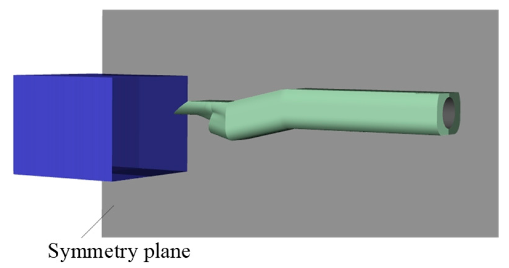
The test equipment studied in this paper and the inlet of its model feature a complex three-dimensional configuration. Therefore, it is necessary to select specific cross-sections to present the reconstruction/prediction results. For the convenience of comparing the wave system structure of the compression surface and the flow field changes along the entire path, the model’s symmetry plane at x = 0 mm is selected as the prediction location. The model’s symmetry plane is shown in Figure 7.

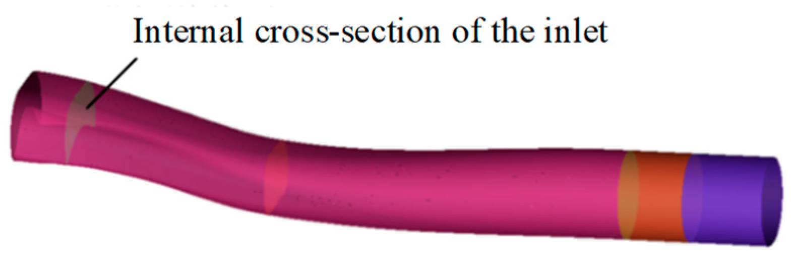
Meanwhile, the along-the-path cross-sections of the inlet at y = 607.56 mm are selected to display the cross-sectional flow of the inlet, with their specific positions shown in Figure 8 below. It should be noted that these cross-sections are chosen arbitrarily, and the prediction method and conclusions of this paper are also applicable to other cross-sections.

5.1. POD Modal Selection and Flow Field Reduced-Order Reconstruction

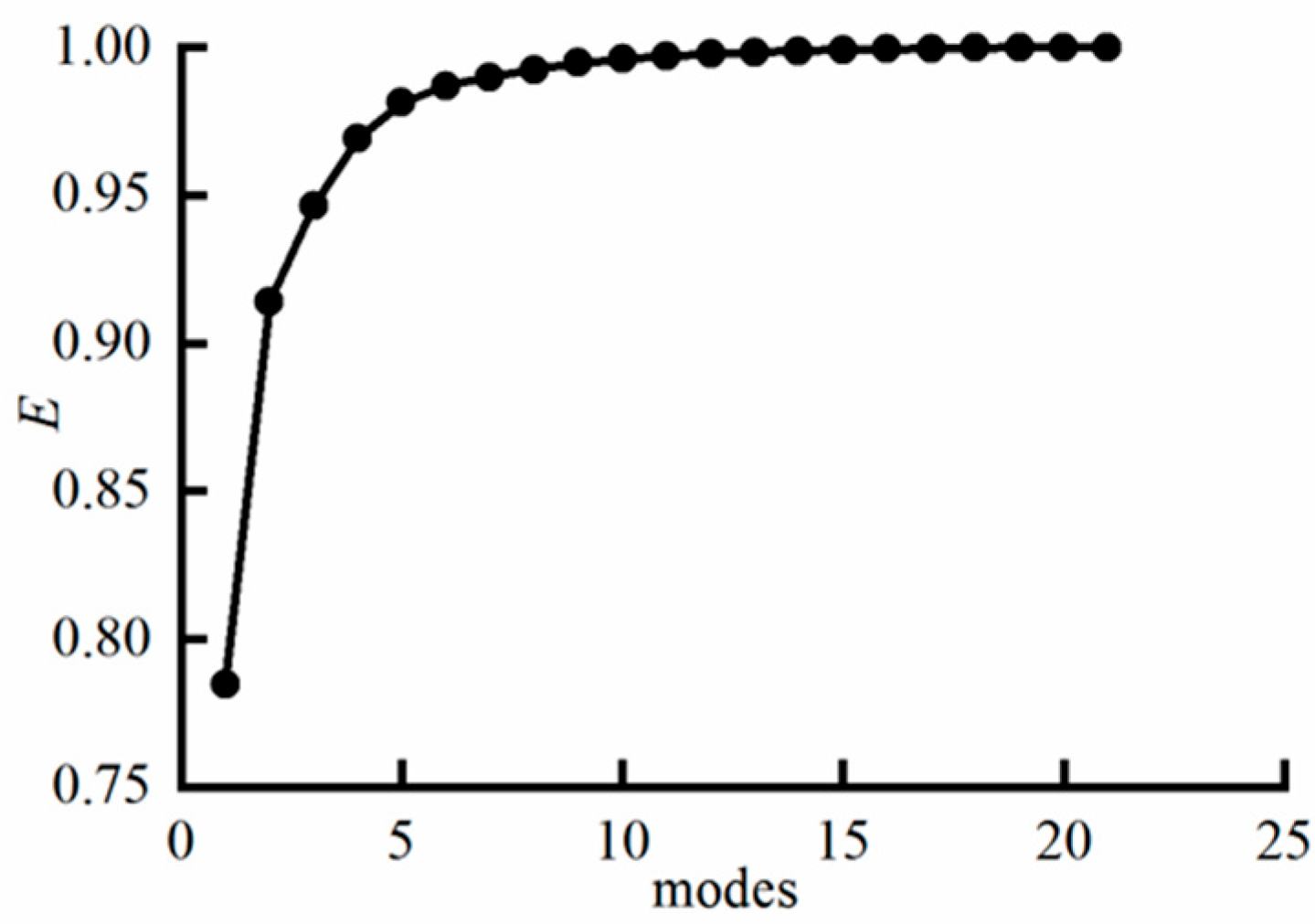
First, a reduced-order study on the Mach number distribution model of the test section under different angles of attack was conducted. Figure 9 shows the energy distribution of each POD mode in the central plane. Among them, the first-order POD mode contains approximately 78% of the total energy, while the energy proportion of the second-order POD mode drops rapidly to about 13%; the total energy proportion of the first two POD modes reaches more than 90%. When the number of POD modes is nine, the total energy proportion of the first nine POD modes exceeds 99%.

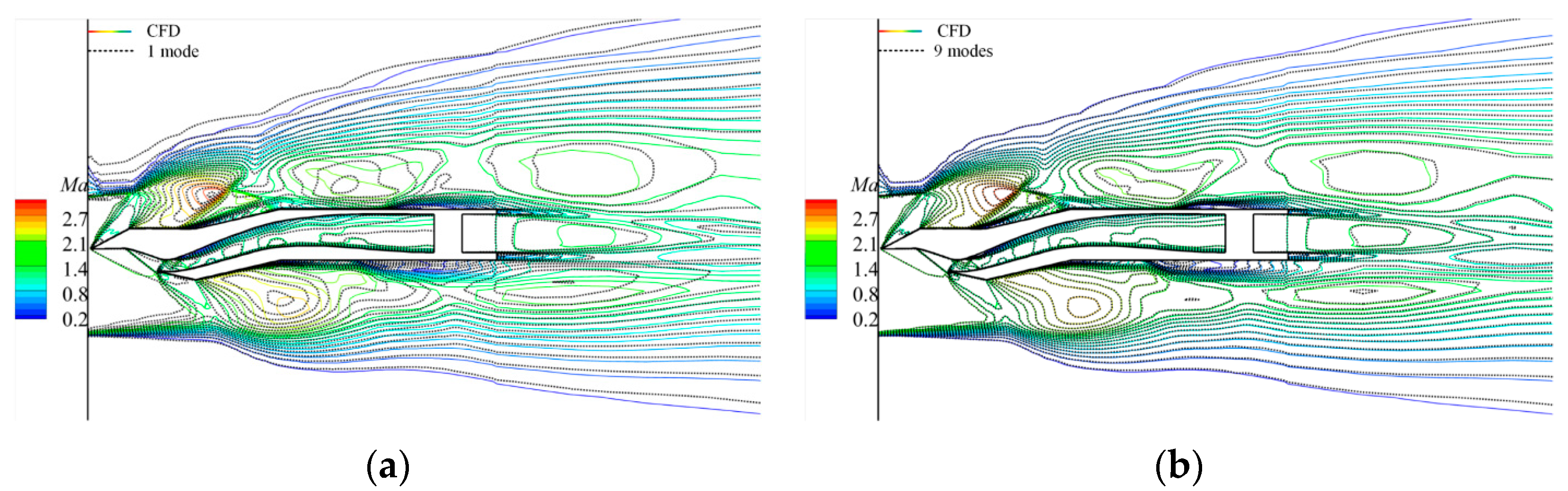
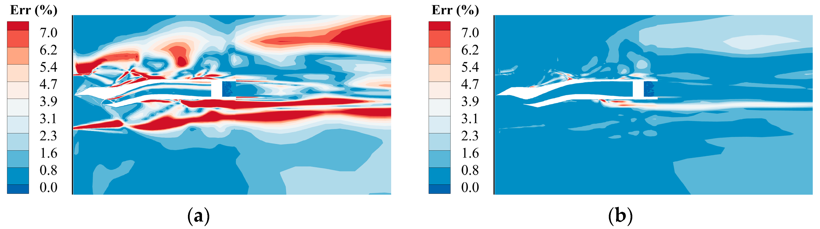
Figure 10 and Figure 11 present the reduced-order reconstruction results and the relative error Err, which is defined as the difference between the reconstructed value and the CFD result divided by the CFD result for the Mach number in the symmetry plane when the angle of attack is +4°. It can be observed that the first-order POD mode can accurately characterize the flow field structure in some regions, but there is a significant discrepancy between this result and the CFD calculation result, with a reconstruction error of 9.16% at this point. When the number of modes increases to nine, the reconstruction result almost completely overlaps with the CFD calculation result. The relative error Err decreases significantly; the reconstruction error is 1.83%, indicating high accuracy of the reduced-order reconstruction. Therefore, this paper selects the first nine POD modes for the study of flow field prediction/reconstruction.

5.2. Rapid Prediction of Flow Field Under Different Angles of Attack

Based on the POD model reduction, studies on the rapid prediction methods of POD-RBF and POD-BPNN were conducted, and the flow field structure of the test under different angles of attack was predicted.

Two operating conditions with angles of attack (AOAs) of −2.5° and +2.5° were selected to verify the prediction capability of this method. Under both conditions, the incoming flow Mach number is 2.0, and the simulated altitude is 15 km. Neither of these two operating conditions is a sample point operating condition.

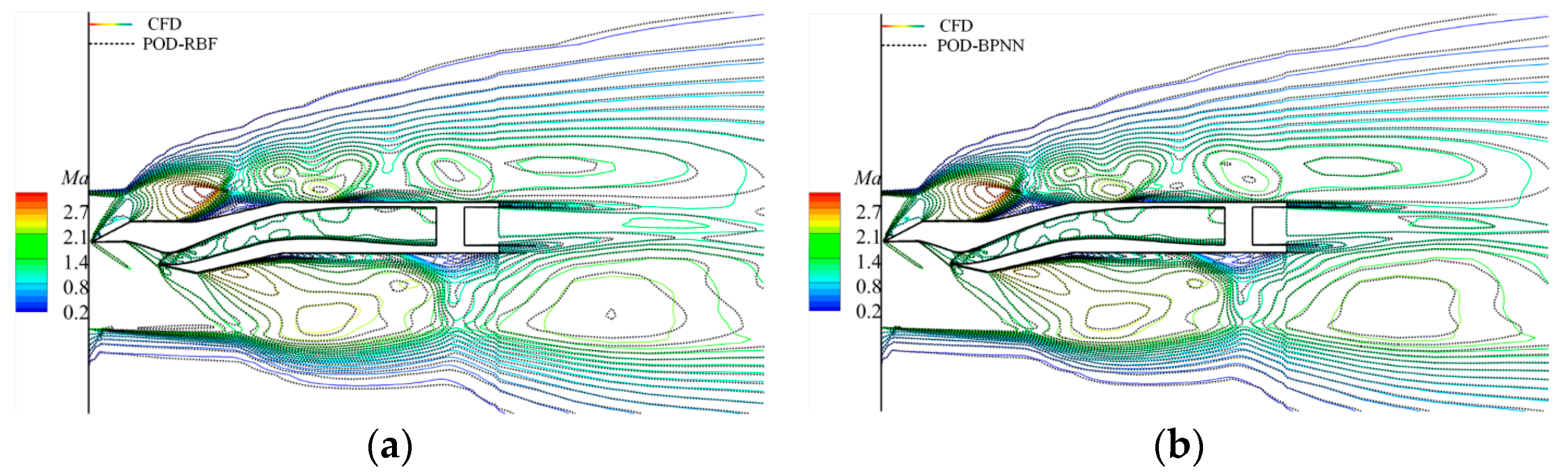
Figure 12 presents the comparison diagram between the prediction results and the Mach number distribution obtained by CFD in the symmetry plane when the AOA = −2.5°. For the prediction, the number of POD modes was set to nine. In the figure, the colored solid lines represent the CFD numerical calculation results, and the black dotted lines represent the prediction results of POD-RBF or POD-BPNN. It can be observed that both rapid prediction methods can accurately characterize the wave system structure of the internal and external flows of the inlet as well as the contour distribution of the external flow field around the inlet. The prediction errors of POD-RBF and POD-BPNN are 4.18% and 3.07%, respectively, with POD-BPNN showing slightly better accuracy. On a personal computer, the time required for flow field prediction is 0.04 s, which meets the real-time requirement for online prediction. By contrast, the CFD takes 43,200 s when using 40 cores for parallel computing using the High-Performance Computing Center of Nanjing University of Aeronautics and Astronautics.

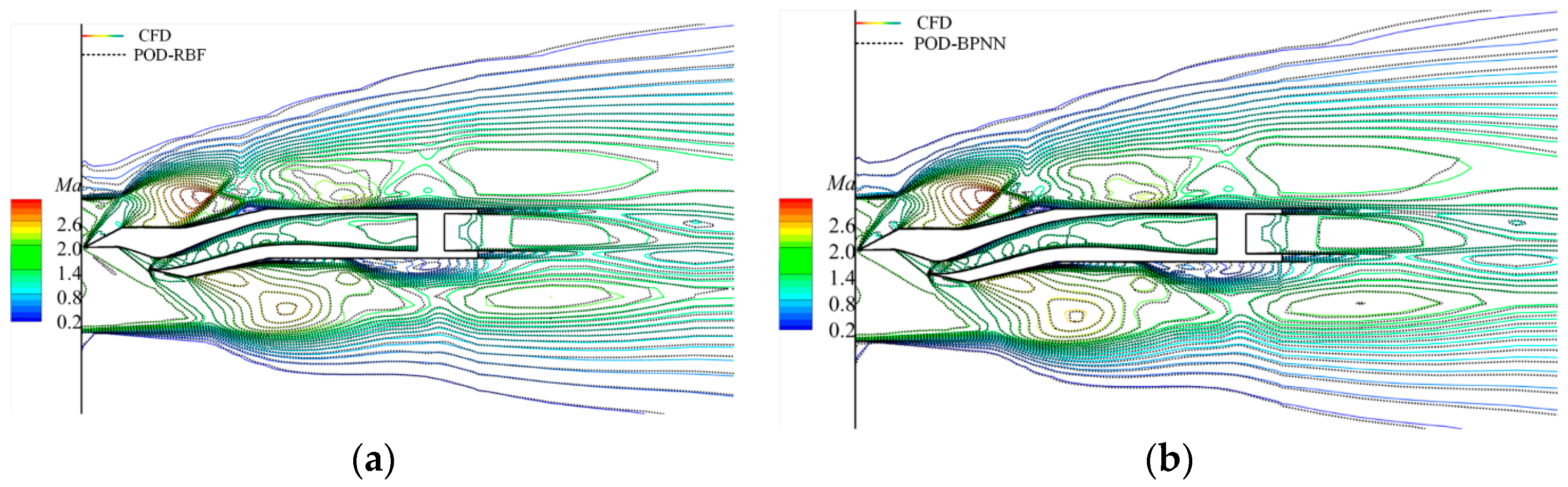
Figure 13 presents the comparison diagram between the Mach number distributions obtained by the rapid prediction methods and CFD in the symmetry plane when the AOA = +2.5°. Similarly, it can be observed that the prediction results almost coincide with the CFD results, with the prediction errors of POD-RBF and POD-BPNN being 4.19% and 3.42%, respectively. On a personal computer, the time required for flow field prediction is only 0.05 s. It can be seen that the rapid prediction methods are accurate and fast.

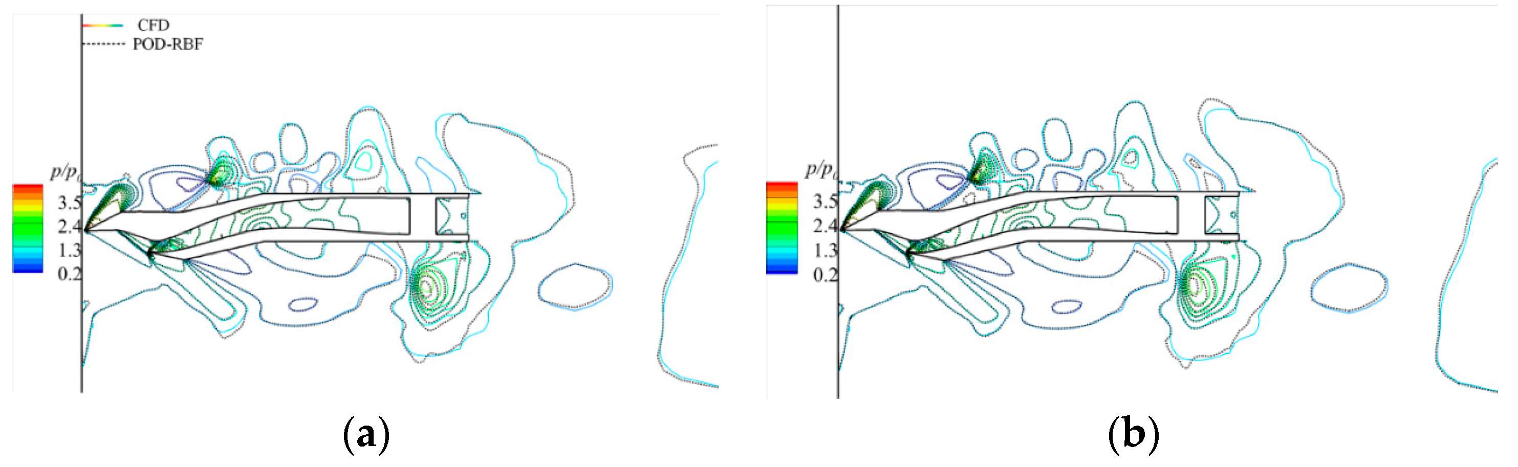
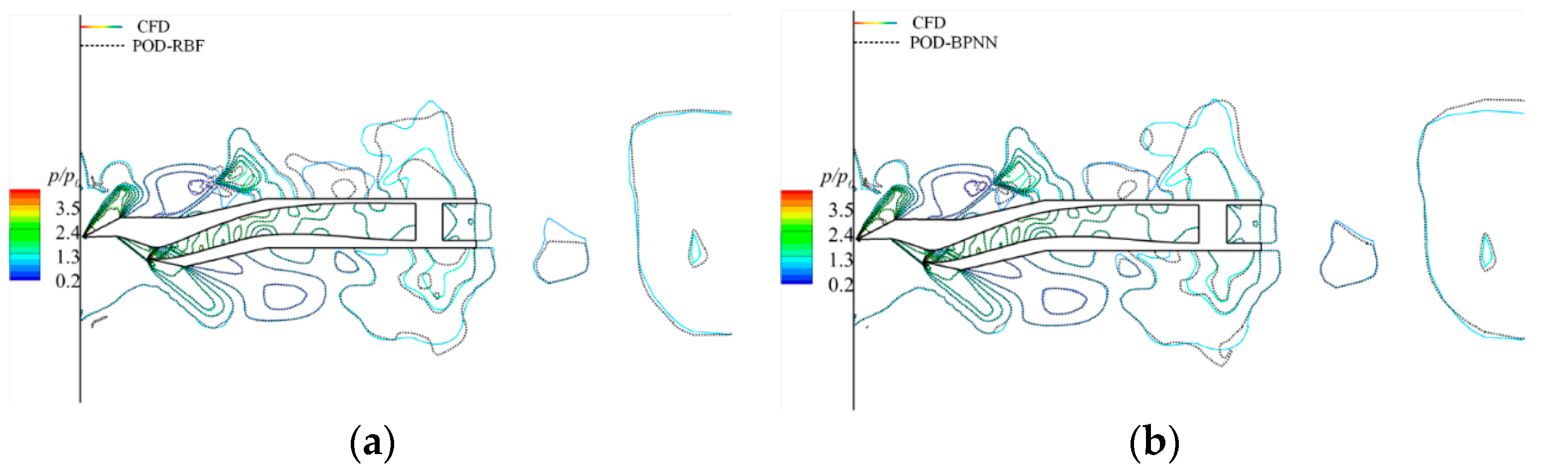
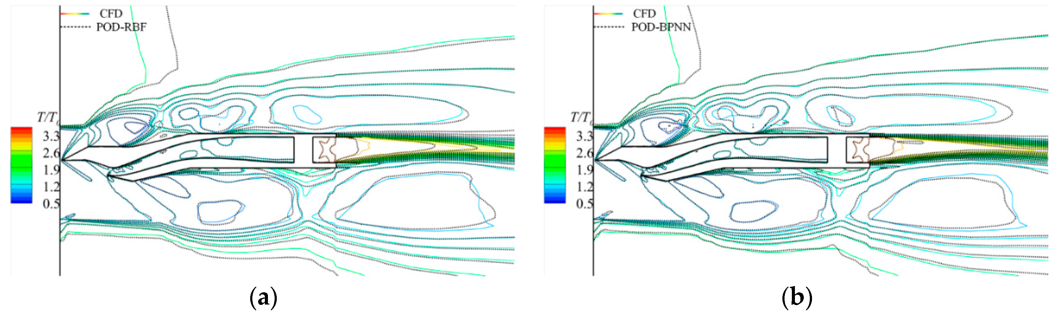
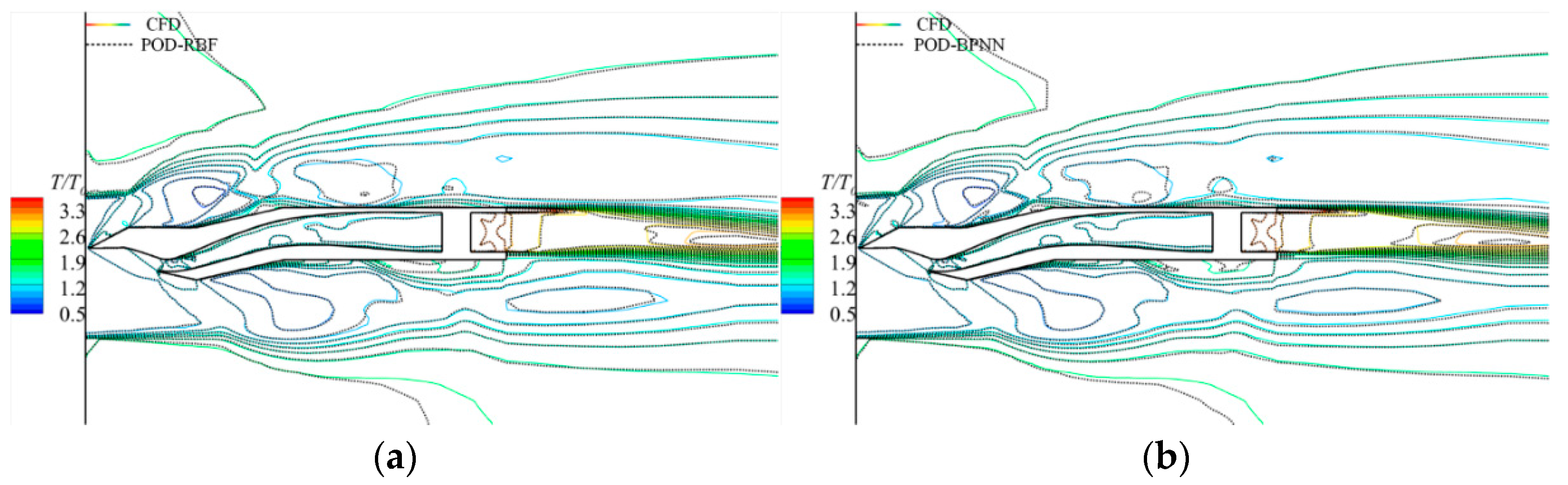
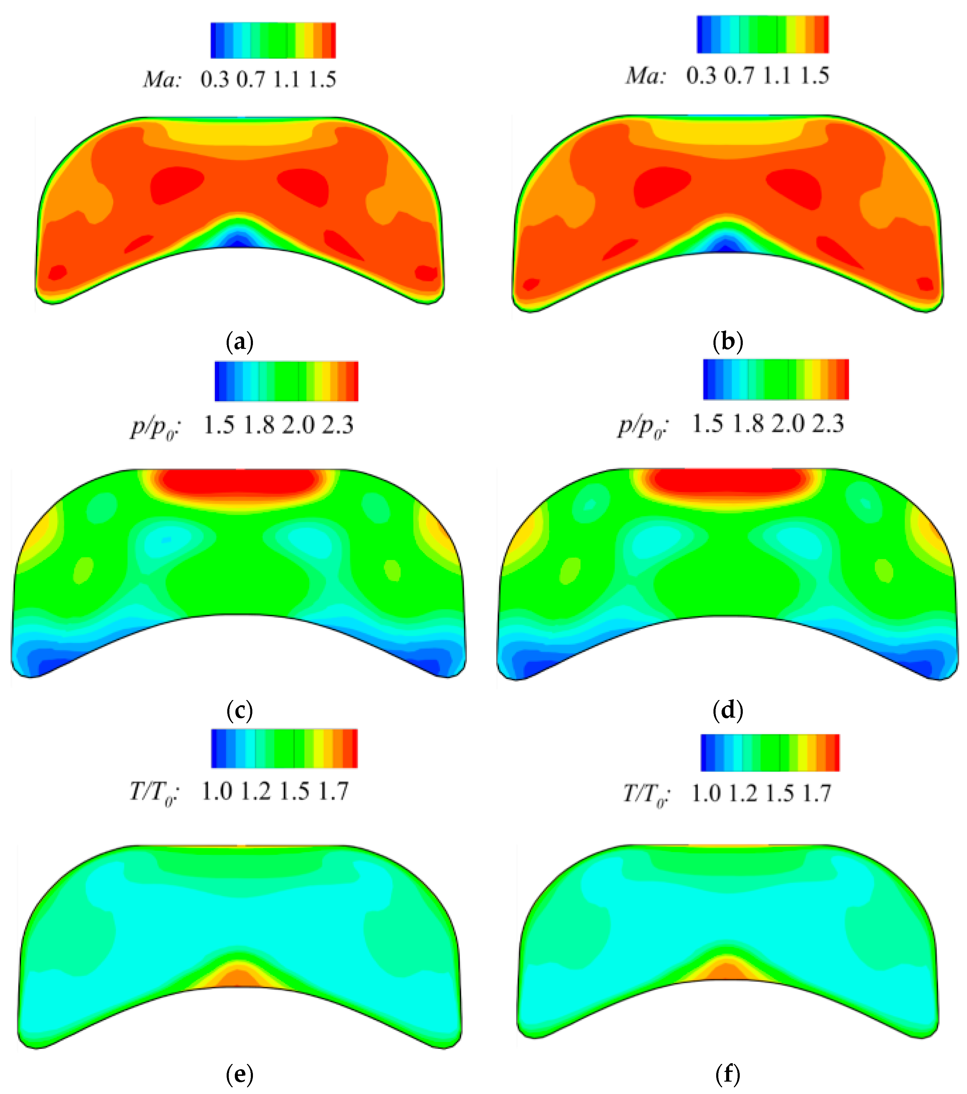
Meanwhile, the study further indicates that these two prediction methods can also very accurately predict the distributions of pressure fields and temperature fields under different angles of attack. In Figure 14, Figure 15, Figure 16 and Figure 17, both the pressure fields and temperature fields are non-dimensionalized using incoming flow parameters. Overall, both methods can accurately predict the wave system structures of the internal flow in the test section and the internal and external flows of the inlet, with the prediction results showing good agreement with the CFD simulation results. Generally speaking, POD-BPNN performs better than POD-RBF in predicting pressure fields. Under the two operating conditions, the average error of POD-RBF is 2.56%, while that of POD-BPNN is 1.52%; the latter has an error 40.63% lower than the former. In terms of temperature field prediction, the average prediction error of POD-BPNN under the two operating conditions is 1.93%, and that of POD-RBF is 2.58%. The average error of POD-BPNN is 25.19% lower than that of POD-RBF. From the perspective of spatial distribution, the regions with the largest differences between the prediction results and the CFD results are mainly concentrated in the external flow of the inlet and the wake region.

The central cross-section of the overall flow can well demonstrate the inlet wave system structure and the internal flow characteristics of the inlet in the overall test flow. However, in such tests, the flow characteristics at the inlet entrance are also a region of concern. Therefore, predicting the flow field distribution at the inlet entrance has very practical significance.

Figure 18 shows the prediction results of Mach number, pressure, and temperature distributions in the inlet cross-section when the angle of attack is +2.5°. In the figure, the contour plots on the left are the CFD numerical calculation results, and the contour plots on the right are the POD-RBF prediction results. It can be observed that at an angle of attack of +2.5°, a relatively large low-Mach-number region is generated behind the central bump, and POD-RBF can still accurately predict the distributions of Mach number, static pressure, and static temperature at this cross-section. The prediction error of each parameter is less than 3.8%, and the prediction time is less than 0.02 s.

5.3. Rapid Prediction of Flow Field Under Different Mach Numbers

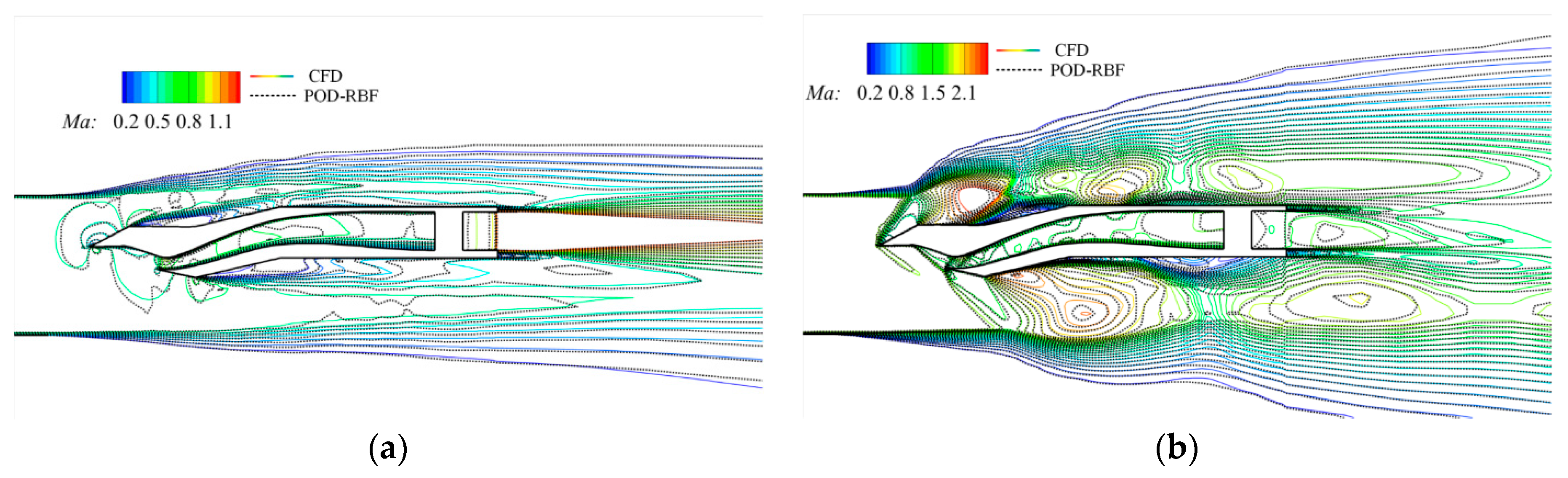
Taking the incoming flow Mach number as the prediction variable, this study assesses the prediction of complex flow fields under different Mach numbers in experiments. Meanwhile, two operating conditions with Mach numbers of 0.65 and 1.85 are selected to verify the prediction capability of the fast method, which basically represents the ability of the fast method to characterize and predict flows under subsonic and supersonic operating conditions. The flight altitude is set to 15 km, and the angle of attack is set to 0 degrees.

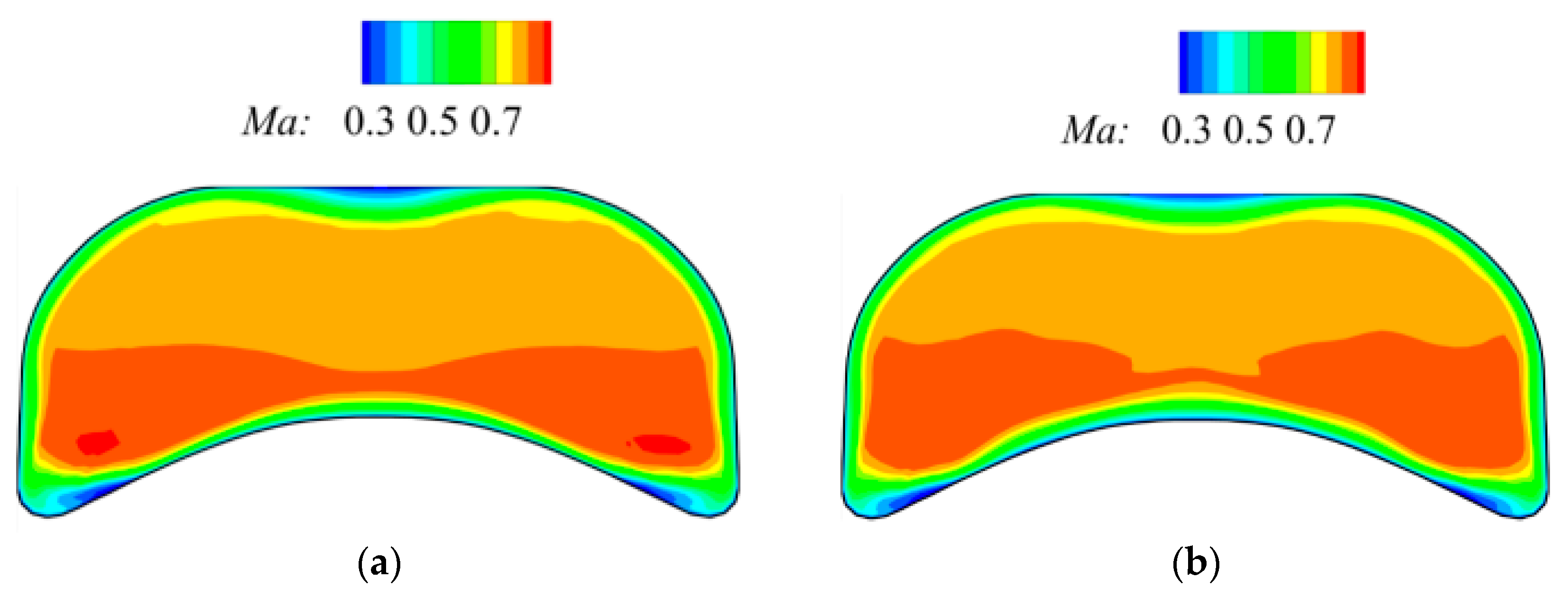
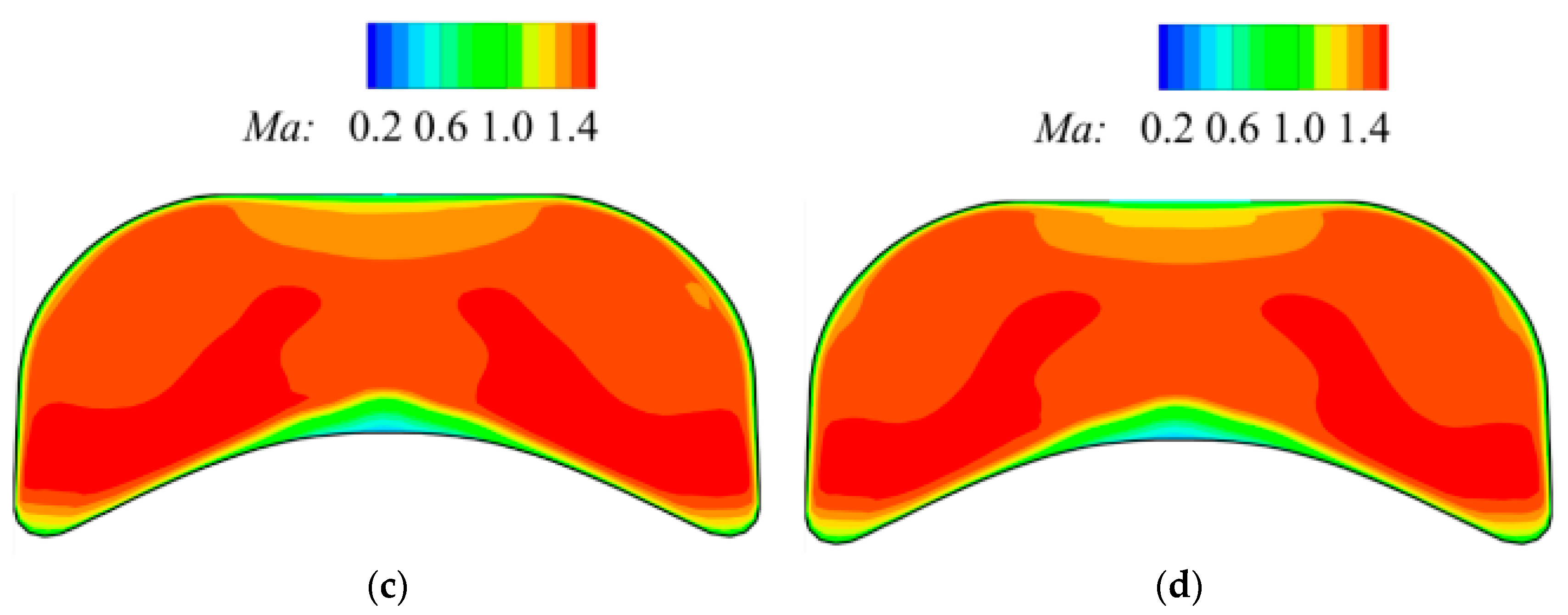
Figure 19 presents a comparison chart of the Mach number distribution on the model’s symmetry plane under the incoming flow Mach numbers of the two operating conditions. In the figure, the colored solid lines represent the CFD numerical calculation results, and the black dotted lines represent the POD-RBF prediction results. It can be seen that under the supersonic condition of Operating Condition 2, the fast method can not only accurately predict the shock wave system structure of the inlet but can also accurately predict the external flow field distribution around the integrated model, including the top separation zone. The prediction results are highly consistent with the CFD results. In addition, the study found that the prediction error of Operating Condition 1 is 5.31%, while that of Operating Condition 2 is 4.55%; the POD-RBF method shows a smaller error under supersonic conditions. A similar pattern is also observed in the prediction of the cross-sectional Mach number distribution in Figure 20. Under the two operating conditions of Ma = 0.65 and Ma = 1.85, the prediction errors of the inlet cross-section are 3.87% and 1.57%, respectively, with a smaller prediction error in the supersonic case. However, in general, the POD-RBF method can still relatively accurately predict the subsonic or supersonic flow fields inside the test section.

6. Conclusions

In this paper, POD model order reduction is adopted, and combined with RBF and BPNN methods, the POD-RBF and POD-BPNN rapid prediction methods are established, respectively. Moreover, rapid prediction research under different angles of attack and incoming flow Mach numbers is carried out for the free jet test. The main conclusions are as follows:

(1)

The model order reduction results show that truncating the POD at the ninth mode can characterize the structure of the sample flow field. The reconstruction result of the ninth mode almost coincides with the result of the CFD full-order model, with a small error of 1.83%, which has reference value for this type of flow prediction.

(2)

In terms of predicting Mach number, static pressure, and temperature, both methods can relatively accurately predict the flow characteristics under different flow conditions. On the basis of the same model order reduction and number of modes, POD-BPNN generally has lower errors than POD-RBF, showing superior prediction performance.

(3)

When the POD-RBF method is used to predict the flow field structure under different Mach numbers, the error in the subsonic regime is larger than that in the supersonic regime. In the supersonic case, both methods can accurately predict the wave system structure and separation zone of the flow field.

(4)

In addition to the central cross-section, both POD-RBF and POD-BPNN can accurately predict the flow field parameter distribution in any cross-section of the inlet, which provides an idea for the real-time monitoring of inlet flow field distortion. In terms of prediction time, the prediction times of all results in this paper are less than 1.0 s, meeting the requirements of accurate and rapid prediction. Therefore, this method can lay an important foundation for the physical “twin” of future free jet tests.