Article

Observer-Based Remote Conductivity Variable-Parameter Sliding Mode Control for Water–Fertilizer Integration Machines Using Recursive Least Squares Adaptive Estimation

1
College of Mechanical and Electrical Engineering, Shihezi University, Shihezi 832003, China
2
College of Information Science and Technology, Shihezi University, Shihezi 832003, China
3
Xinjiang Production and Construction Corps Key Laboratory of Modern Agricultural Machinery, Shihezi 832003, China
4
Key Laboratory of Northwest Agricultural Equipment, Ministry of Agriculture and Rural Affairs, Shihezi 832003, China
5
Corps Energy Development Research Institute, Shihezi University, Shihezi 832003, China
*
Author to whom correspondence should be addressed.
Appl. Sci. 2025, 15(9), 4993; https://doi.org/10.3390/app15094993
Submission received: 17 March 2025 / Revised: 23 April 2025 / Accepted: 28 April 2025 / Published: 30 April 2025
(This article belongs to the Collection Agriculture 4.0: From Precision Agriculture to Smart Agriculture)

Abstract

:
In remote conductivity control for water–fertilizer integration systems, challenges such as long-distance nonlinearities and variable parameters can lead to fertilization inaccuracies, including over-irrigation and uneven distribution, affecting both productivity and environmental sustainability. To mitigate these issues, this study proposes a variable-parameter sliding mode control (VSMC) strategy, combined with an adaptive observer based on Recursive Least Squares (RLS) to estimate system inertia and load torque in real time. This allows for dynamic adjustment of the sliding surface parameters, ensuring robust control even under varying operating conditions. Two parameter derivation approaches—analytical modeling and data-driven fitting—are evaluated. Field tests demonstrate that VSMC outperforms the Proportional–Integral (PI) and conventional sliding mode control (SMC) methods in maintaining target electrical conductivity (EC) levels. Specifically, for a target EC of 1.4 mS/cm, VSMC stabilizes the system to within 1.18–1.60 mS/cm in 95 s, with a 14.3% overshoot, well within agronomic tolerance. In regional irrigation trials, VSMC significantly improves fertilizer uniformity, reducing the standard deviation of potassium nitrate distribution from 2.14 (PI) to 0.59. The simulation and experimental results validate the effectiveness and robustness of the proposed method, highlighting its potential to enhance agronomic efficiency and reduce environmental impact.

1. Introduction

1.1. Remote Conductivity Control in Water–Fertilizer Integration

The remote conductivity control system for water and fertilizer integration machines has garnered significant attention due to its application in various fields such as agriculture and horticulture [1,2]. This system plays a crucial role in optimizing water and fertilizer management, thereby enhancing crop yield and quality while conserving resources [3,4]. Comprising water supply, fertilization, drip irrigation, and monitoring components, this integrated system offers precise control over water and nutrient delivery, ensuring optimal plant growth [5,6].

1.2. Challenges in PMSM Servo Systems

The permanent magnet synchronous motor servo system (PMSM) has been widely applied in many fields such as control systems, agriculture, and engineering, and has attracted widespread attention from both industrial and academic communities [7,8]. The performance requirements for this system are becoming increasingly stringent [9,10]. Traditional PI control relies on precise mathematical models, and changes in operating conditions or motor parameters significantly affect its performance [11,12]. To enhance the robustness of servo systems, many modern control algorithms have been applied, such as adaptive control, fuzzy logic control (FLC), and sliding mode control (SMC) [13,14]. Recent studies comparing these techniques in PMSM applications show that while adaptive control improves parameter tuning under dynamic loads, FLC enhances nonlinear decision making, and SMC remains superior in terms of disturbance rejection and robustness under parameter uncertainties [15,16].

1.3. Advancements in Sliding Mode Control

In recent years, numerous scholars have combined observers with SMC to further enhance the performance of sliding mode controllers by observing disturbances [17,18]. For instance, some scholars have proposed methods to enhance the robustness of sliding mode controllers applied to permanent magnet linear synchronous motor servo systems [19]. Truong et al. designed an adaptive backstepping complementary sliding mode controller based on a disturbance observer to reduce the impact of parameter or load variations on system control performance [20]. Xu H. et al. used internal model control to achieve a fast and overshoot-free step velocity response for linear motors and combined a disturbance observer with a sliding mode controller to improve system robustness, though this method was structurally complex [21]. Xu B.L. et al. employed adaptive control to estimate the upper bound of uncertain system parameters, designing an adaptive non-singular fast terminal sliding mode to enhance system robustness, with a step position response able to quickly follow the set value in an overshoot-free manner [22].
In PMSM control systems, step-type or sinusoidal speed commands, or sinusoidal position commands, are typically used to verify control performance [23]. Numerous scholars have extensively studied enhancing the robustness of SMC under such conditions [24,25]. However, there is less research on step-type position response, and most studies have not verified the robustness of SMC against changes in rotational inertia [26]. For example, one study [27] used the disturbance estimates observed by a state observer as a feedforward compensation term to correct the output of SMC, improving the sliding mode control’s robustness against internal parameter perturbations. This enabled the PMSM servo system’s position response to better follow sinusoidal command signals even when rotational inertia varied, but there was often overshoot when following step command signals [28]. Another study employed the real-time adjustment of SMC’s output based on observed load torque values to enhance its robustness [29]. This method achieved good results in suppressing speed step response overshoot and speeding up response time, but it did not specify whether control performance would be affected by changes in rotational inertia [30,31].

1.4. Research Gap and Proposed Solution

Despite advancements in sliding mode control (SMC) for step-type position responses, a significant gap remains in addressing the robustness of SMC under varying rotational inertia conditions. Specifically, current research lacks comprehensive methodologies to ensure the consistent and reliable performance of SMC algorithms when applied to systems with dynamically changing rotational inertia. This paper aims to fill this gap by proposing a variable-parameter sliding mode control (VSMC) method that integrates inertia and load torque observations using a least squares observer. This approach allows for the adaptive adjustment of control parameters, enhancing the robustness of position control in systems where rotational inertia fluctuates.
Based on the above analysis, a variable-parameter sliding mode controller (VSMC) based on a recursive least squares (RLS) observer is designed to enhance the robustness of PMSM servo systems, ensuring that these systems maintain an optimal step position response performance even when parameters such as rotational inertia change. VSMC uses the rotational inertia and load torque values observed by the RLS observer to adjust its sliding mode surface parameters, achieving variable parameter control. Simulations and experiments indicate that this method effectively improves the step position response performance of PMSM servo systems and is insensitive to changes in rotational inertia, demonstrating a strong robustness.

1.5. Objectives

To address the limitations of conventional PI and fixed-parameter sliding mode controllers under dynamic system conditions, this study aims to achieve the following:
  • Develop a VSMC strategy to enhance the robustness of PMSM servo systems used in water–fertilizer integration equipment.
  • Design a recursive least squares (RLS)-based observer to estimate real-time system parameters, including rotational inertia and load torque.
  • Adaptively adjust the sliding surface parameters in the VSMC using the observer’s output to maintain control accuracy under varying operating conditions.
  • Compare two parameter derivation strategies—analytical modeling and data-driven fitting—for determining sliding mode parameters.
  • Validate the proposed method through simulations and field experiments by assessing its performance in maintaining target conductivity and improving fertilizer distribution uniformity.

2. Materials and Methods

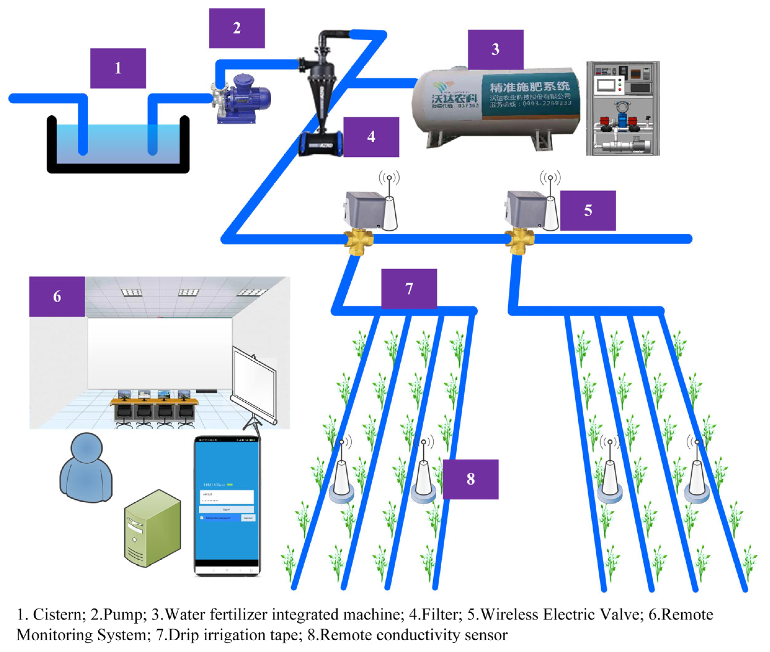
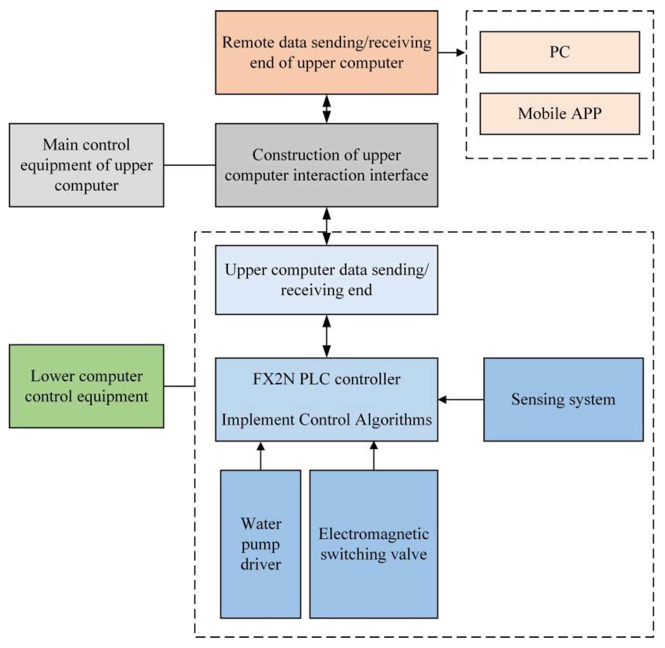
2.1. Remote Conductivity Control System for Water and Fertilizer Integration Machine

The remote conductivity control system for a water and fertilizer integration machine is shown in Figure 1. The system consists of a control section and a monitoring section. The control section includes water supply components and fertilization components, equipped with response facilities such as filters, fertilizer storage tanks, pumps, pipelines, drip irrigation belts, and wireless electric control valves. The monitoring section includes remote conductivity sensors, pressure sensors, flow sensors, and others. Data transmission between the control and monitoring sections is realized through the LoRa wireless communication protocol, which provides long-distance, low-power, and stable data exchange capabilities, suitable for agricultural field environments.
The water and fertilizer integration system consists of multiple coordinated subsystems. The pumping unit uses a hose pump with a starting torque of 230 N·m, a maximum flow rate of 5310 L/h, and a maximum operating pressure of 0.8 MPa. The pump is driven by a frequency converter, enabling variable flow control according to real-time demands.
The fertilizer supply unit is designed for the proportional mixing and delivery of fertilizers such as urea, monoammonium phosphate, and potassium phosphate. It features a paddle stirring mechanism, driven by a three-phase asynchronous motor with a rated power of 0.75 kW. The stirring rod has a shaft diameter of 1 m and is equipped with two straight blades, ensuring an adequate mixing efficiency. Fertilizer is transported using a single-phase screw self-priming pump rated at 1.8 kW, with a suction range of 10–25 m and a flow rate of 9 m3/h. The unit supports a maximum stirring volume of 1.5 m3.
For flow measurement, an electromagnetic flow sensor with a measurement accuracy of ±0.5% is integrated into the system, ensuring precise fertilizer dosing.
The power supply unit converts on-site three-phase power into 220 V, 24 V, and 12 V outputs, providing stable power to the control, monitoring, and actuation components throughout the system.
An implementation diagram of the remote conductivity control system for the water and fertilizer integration machine is shown in Figure 2. The lower computer, based on a programmable logic controller (PLC), is responsible for monitoring sensor signals such as flow rate, pressure, and pipeline EC values, as well as controlling the water pump, fertilizer pump, and solenoid valves. The upper computer, developed using a combination of Python 3.8 and LabVIEW 2020 64-bit, communicates wirelessly with the cloud platform via the LoRa protocol, sends control signals to the lower computer, and uploads sensor data and component status in real time. The communication between the upper and lower computers adopts the Modbus RTU protocol, ensuring reliable and standardized data exchange.

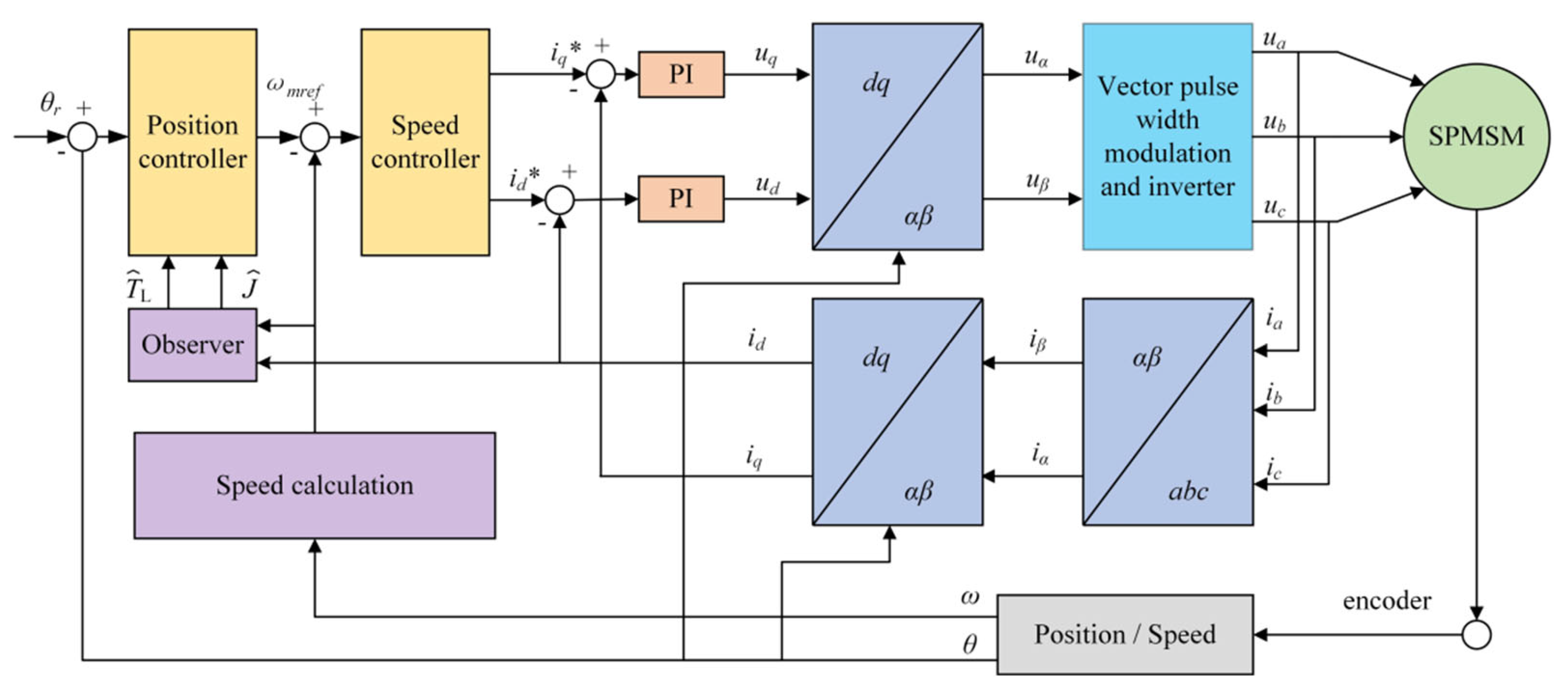
2.2. Design of the Variable-Parameter Sliding Mode Position Controller

A control block diagram of the position, speed, and current three-loop control system is shown in Figure 3. Taking the PMSM as an example, the id = 0 control strategy is adopted. The main purpose of this paper is to investigate the robustness of the sliding mode position controller (outer loop) to parameter variations. To achieve this, it is necessary to ensure that the inner loops are minimally affected by parameter changes, thereby eliminating their influence on the robustness of the system’s position control. Therefore, a fuzzy logic controller, known for its strong robustness and fast dynamic response, is employed in the speed loop.
In the dq coordinate system, the mathematical model of the PMSM is shown in Equation (1), which describes the dynamic behavior of the motor in terms of stator voltages, currents, and rotor position. This model is based on the commonly adopted formulation presented in [32], which provides a detailed derivation of PMSM dynamics under field-oriented control assumptions.
u d = R s ( i d i d ) + L d d ( i d i d ) d t ω r L q ( i q i q ) u q = R s ( i q i q ) + L q d ( i q i q ) d t + ω r L d ( i d i d ) + ω r ψ f T e = 3 2 p [ ψ f i q + ( L d L q ) i d i q ] J d ω m d t = T e T L B m ω m T f sgn ( ω m ) ω e = d θ / d t
In the equation, uq and ud represent the quadrature and direct-axis components of the stator voltage, respectively; iq and id represent the quadrature and direct-axis components of the stator current, respectively; iq* and id* represent the reference values of the d-axis and q-axis currents, respectively; Ld and Lq represent the direct and quadrature synchronous inductances, respectively; Rs is the stator winding resistance; ωr is the electrical angular velocity; ωm is the mechanical angular velocity, where ωr = p*ωm and p is the pole pair number; ψf is the excitation flux of the permanent magnet; Bm is the viscous friction coefficient; θ is the mechanical position angle of the motor rotor; J is the system’s moment of inertia; Te is the electromagnetic torque; TL is the load torque; and Tf is the friction torque.
The state variables of the PMSM system are selected as follows:
x 1 = θ ref θ x 2 = x ˙ 1 = θ ˙ ini ω m
In the equation, θref is the position reference value and θini is the instantaneous position error, which is the difference between θref and θ at the instant when the reference undergoes a step change.
The sliding mode surface of the system is designed as follows:
s = c x 1 + x 2 = 0
In the equation, c is the sliding mode surface parameter, which is a positive constant.
To enhance the quality of the reaching phase in sliding mode control, this paper adopts exponential reaching law, as follows:
s ˙ = ε sgn ( s ) q s
In the equation, ε and q are positive constants. Sliding mode control may exhibit a chattering phenomenon, and in general, reducing the value of ε appropriately can mitigate chattering.
According to Equations (2) and (3), the expansion of s ˙ is as follows:
s ˙ = c x ˙ 1 + x ˙ 2 = c x 2 + θ ˙ ini ω ˙ m
Substituting Equation (5) into Equation (4) yields the output of the fixed-parameter sliding mode position controller, i.e., the speed reference value is as follows:
ω mref = θ ˙ ini + ( c x 2 + ε sgn ( s ) + q s ) d t
Because θ ˙ ini is an impulse function, it becomes zero after the initial moment, thus, Equation (6) can be simplified.
ω mref = ( c x 2 + ε sgn ( s ) + q s ) d t
Clearly, ω mref is generated by the output of the integrator. The integrator acts as a filter to smooth the alternating signal, thus suppressing the chattering of SMC.
The above is the basic principle of fixed-parameter sliding mode position control. Next, the design idea of variable-parameter sliding mode control (VSMC) will be introduced.
Following this, the design concept of the system phase point (x1, x2) lies on the positive half-axis of x1. Under sliding mode control, its trajectory is shown as the red line in Figure 4.
Let x1(t0) denote the value of the state variable x1 when the phase point first reaches the sliding mode surface (corresponding to point A in Figure 2). From Equations (2) and (3), we can infer the trend of the changes in x1 and x2 during the sliding mode motion process as follows:
x 1 ( t ) = x 1 ( t 0 ) e c t x 2 ( t ) = c x 1 ( t 0 ) e c t
From Equation (8), it can be observed that, by adjusting the parameter c, the speed at which x1 approaches zero can be controlled. The larger the c, the faster the approach speed, meaning that the speed of the position response increases with the increase in c.
During the position step response process, the approximate variation trend of the given speed ωmref and the actual speed ωm is shown in Figure 5. Segment OB represents the approaching movement, and segment BC represents the sliding mode motion. Point B corresponds to point A in Figure 4. Usually, the stage where the actual speed decreases at the end (segment BC) is referred to as the positioning stage. The motion equation during the positioning stage is given by Equation (9), where the acceleration dωm/dt is negative.
d ω m d t = T e T L B m ω m T f sgn ( ω m ) J
The maximum rate of change in speed during this stage is given by Equation (10).
d ω m d t max = T e max + T L max + B m ω m + T f J min
For typical motors, the comprehensive friction torque is much smaller compared to the maximum value of electromagnetic torque, so Equation (10) can be further simplified to the following:
| d ω m d t | max = T emax + T L J
As observed, it is limited by the maximum value of electromagnetic torque Temax, the load torque TL, and the system inertia J, and cannot increase indefinitely.
Analyzing Figure 4 and Figure 5, point B in Figure 5 corresponds to point A in Figure 4, i.e., during the positioning stage, the phase point undergoes sliding mode motion. Combining Equations (2) and (8), let the average rate of decrease in the given speed during the positioning stage be as follows:
| d ω mref d t | avg = c 2 x 1 ( t 0 ) 2
From Equation (12), it is evident that, the larger the sliding mode surface parameter c, the greater the average rate of decrease in the given speed. When this rate exceeds the maximum rate of change in speed, the actual speed cannot follow the given speed, resulting in overshoot in the position response when the given speed is equal to zero ( ω mref = 0).
The objective of servo system control is to achieve a fast and overshoot-free position response to the given value. From the previous analysis, it is clear that a larger c leads to a faster response, but excessively large c values can cause overshoot. The optimal value of c is the maximum value that ensures no overshoot in the position response, and this optimal value is constrained by the maximum rate of change in speed, which is positively correlated with it. Additionally, Equation (11) indicates that, under constant conditions, the maximum rate of change in speed during the positioning stage is related to TL and J, so the optimal value of parameter c is also related to them.
In a system using fixed-parameter SMC, the value of c remains constant (i.e., the average rate of decrease in the given speed remains constant). When variations in TL and J lead to a maximum rate of change in speed smaller than this average rate, overshoot occurs in the position response. Conversely, the position response cannot follow the given value at the fastest rate. Therefore, fixed-parameter SMC cannot achieve optimal control under any operating conditions; its performance is significantly affected by TL and J, and its robustness is poor. Therefore, this paper proposes a variable-parameter sliding mode position controller, in which the parameter c is dynamically adjusted according to TL, J, and θini. Additionally, when the position reference undergoes a step change, the smaller the θini, the smaller the value of x1(t0). From Equation (12), it is apparent that under constant average rate conditions, reducing x1(t0) allows the value of c to be appropriately increased. Thus, the parameter c should also vary with changes in θini.
In summary, the VSMC proposed in this paper dynamically adjusts its sliding mode surface parameter c according to the values of TL, J, and θini to achieve optimal control under any operating conditions. Clearly, θini can be directly calculated, while TL and J are unknown quantities. Therefore, this paper designs a recursive least squares observer to observe them. The following section will briefly introduce how to utilize this method to obtain their observed values.

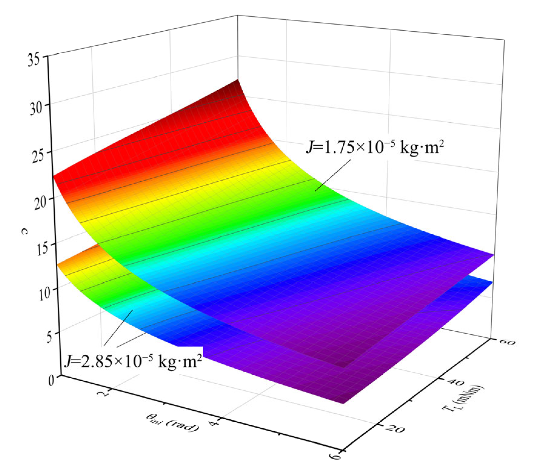
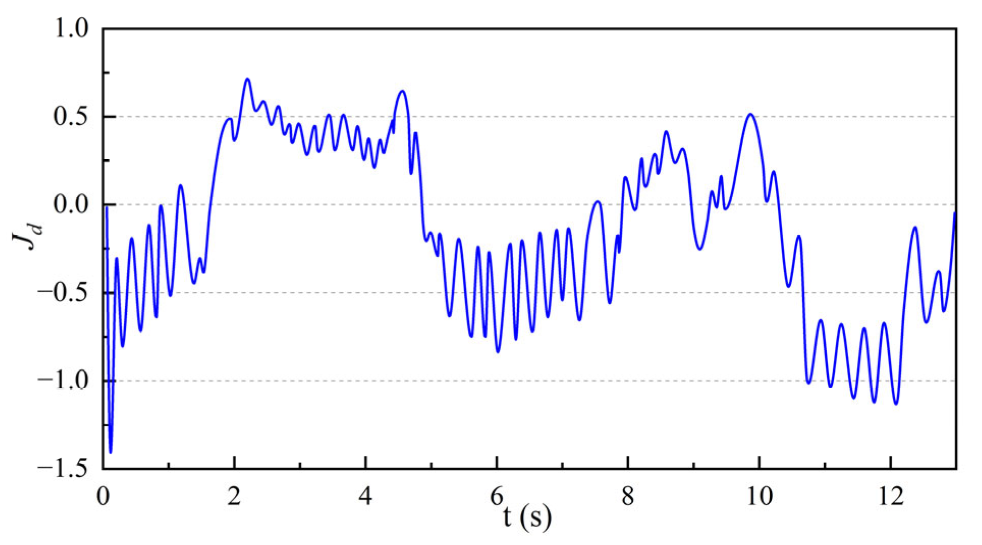
2.3. Design of the Recursive Least Squares Observer

Incorporating the mathematical model of the motor, let us briefly introduce the principle of the recursive least squares (RLS) observer. By performing the Laplace transform on the motion equation of the motor, the motion equation of the motor in the frequency domain can be obtained as follows:
ω m ( s ) = 1 J s + B m ( T e ( s ) T L ( s ) h T f ( s ) )
In the equation, h = s g n ( ω m ) .
After introducing the zero-order hold element, performing the Z-transform on the motion equation of the motor yields its expression, as shown in Equation (14) as follows:
A = 1 e B m T s / J B m B = e B m T s / J C = 1 e B m T s / J B m T L D = 1 e B m T s / J B m T f
The above equation can be solved to obtain the following:
ω m ( z ) = z 1 ( 1 e B m T s / J ) B m ( 1 z 1 e B m T s / J ) × ( T e ( z ) T L ( z ) h T f ( z ) )
where Ts represents the sampling period of the identification algorithm, assuming that within one sampling period, the values of ωm and Te remain constant.
ω m ( k ) = A T e ( k 1 ) B ω m ( k 1 ) C h D
We define the output variable y(k), input column vector x(k), and parameter column vector λ as expressed in Equation (16).
y ( k ) = ω m ( k ) x ( k ) = T e ( k 1 ) , ω m ( k 1 ) , 1 , h T λ = [ A , B , C , D ] T
The relationship between them can be derived from Equation (15), as follows:
y ( k ) = x ( k ) T λ
According to the recursive least squares principle, the identification formula for the observer is given by the following:
K ( N ) = P ( N 1 ) x ( N ) 1 + x ( N ) T P ( N 1 ) x ( N ) y ^ ( N ) = x ( N ) T λ ^ ( N 1 ) e ( N ) = y ( N ) y ^ ( N ) λ ^ ( N ) = λ ^ ( N 1 ) + K ( N ) e ( N ) P ( N ) = P ( N 1 ) K ( N ) x ( N ) T P ( N 1 )
In the equation, K(N) is a 4-dimensional column vector; P(N) is a 4 × 4 covariance matrix; y ^ N is the N-th estimate of the output variable; λ ^ N is the N-th estimate of the parameter column vector; and e(N) represents the deviation caused by using the parameter vector from the previous time step for prediction at the current time step.
During the identification process, the correction value K(N)e(N) is continuously used to adjust the parameter vector estimate. The error between the estimated value and the actual value of parameter vector λ ^ N gradually converges to zero. Eventually, using Equation (19), parameters T ^ L and J ^ can be inversely solved from A ^ , B ^ , and C ^ .
J ^ = ( 1 + B ^ ) T s A ^ ln ( B ^ ) T ^ L = C ^ / A ^
Using the observed values T ^ L and J ^ , combined with θini, the sliding mode control (VSMC) parameter c can be dynamically adjusted. A fitting method is employed to establish the relationship between the three values ( T ^ L , J ^ , and θini), and the parameter c. The fitting process involves conducting a series of simulations under different conditions of TL, J, and θini to obtain the optimal value of c, where the position response does not exhibit overshoot (i.e., the system’s position response can quickly follow the reference value without overshooting).
Once the optimal value is determined, curve fitting is performed using existing data to derive the relationship between TL, J, θini, and c. To simplify the fitting process, θini is initially kept constant to obtain the relationship between c and J under different inertia conditions. Then, keeping J constant, the relationship between c and θini under different inertia conditions is determined. Finally, the two relationships are combined to derive the overall fitting equation.
When θini rad and J are 1.75 × 10⁻⁵ kg·m2 and 2.85 × 10⁻⁵ kg·m2, respectively, the relationship between c and θini determined by the fitting method is shown in Table 1. The relationship between c and TL, J can be expressed as Equation (21).
c = 100000 ( T L ) 3 9400 ( T L ) 2 + 1240 T L + 242 ( J = 1.75 × 10 5 kg m 2 ) c = 100000 ( T L ) 3 + ( 100 T L ) 2 + 550 ( T L ) + 200 ( J = 2.85 × 10 5 kg m 2 )
At different moments of inertia, when TL = 0 N·m and J is constant, the relationship between c and θini is expressed as Equation (22).
c = c 0 2 / θ ini
When J = 1.75 × 10⁻⁵ kg·m2, c0 = 245, and when J = 2.85 × 10⁻⁵ kg·m2, c0 = 200. Combining Equations (21) and (22), the overall relationship between parameter c and TL, J, θini can be obtained.
J = 1.75 × 10 5 kg m 2 c 0 2 / θ ini = 100000 ( T L ) 3 9400 ( T L ) 2 + 1240 T L + 242
J = 2.85 × 10 5 kg m 2 c 0 2 / θ ini = 100000 ( T L ) 3 + ( 100 T L ) 2 + 550 ( T L ) + 200
Under different moments of inertia conditions, the relationship surface between c, TL, and θini determined by the fitting method or analytical analysis is shown in Figure 6.

2.4. Software and Versions

All numerical simulations and control algorithm implementations were performed using MATLAB (version R2021a, MathWorks Inc., Natick, MA, USA). Figures were generated using MATLAB’s built-in plotting functions.

3. Results and Discussion

3.1. Simulation Analysis

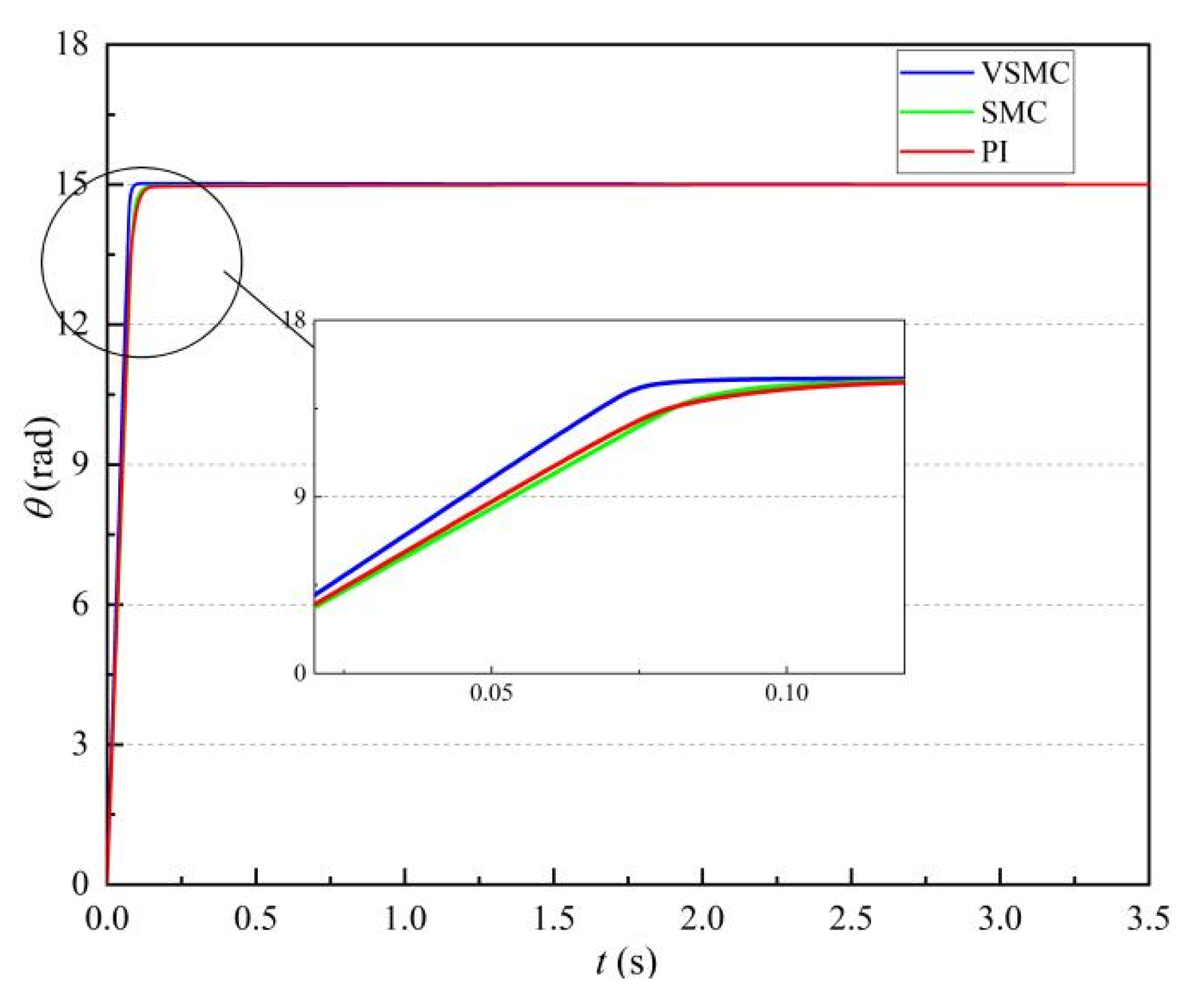
3.1.1. Response Speed Simulation Analysis

In this study, Matlab was utilized to simulate the position servo system, aiming to validate the effectiveness of both the recursive least squares (RLS) observer and the variable-parameter sliding mode control (VSMC). To showcase the efficiency of the designed controllers, a step position of 15 radians was initiated, with the motor operating under no-load conditions. Figure 7 illustrates the position tracking curves for the three control methods, along with an enlarged view spanning from 0.05 to 0.10 s. Upon closer examination, it is evident that the time required for the Proportional–Integral (PI) control to achieve the desired position was approximately 0.14 s, while for SMC, it was 0.12 s, and for VSMC, it was 0.07 s.
While the VSMC strategy demonstrated a superior response speed and shorter settling time compared to the other control methods, it is important to note that the simulation was conducted under no-load conditions. In real applications, external disturbances and varying load conditions can affect the performance of the VSMC strategy. This limitation should be considered, as the control system might need further tuning or compensation mechanisms when applied in real-world scenarios. The impact of load variations on the response speed and accuracy of VSMC in practical applications is an area for future research.
Furthermore, the stability and robustness of the VSMC strategy were examined in this study. The VSMC controller, due to its sliding mode nature, offers robustness against parameter variations and external disturbances. This is because the sliding mode control inherently drives the system to the sliding surface, where the system’s behavior is less sensitive to changes in the system’s parameters. However, while the simulation results demonstrated a good robustness under ideal conditions, the real-world implementation of VSMC may require further validation, particularly under conditions with more significant parameter uncertainties and external disturbances.

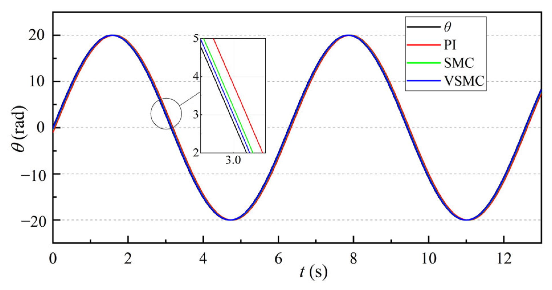
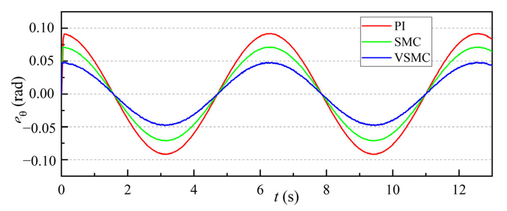
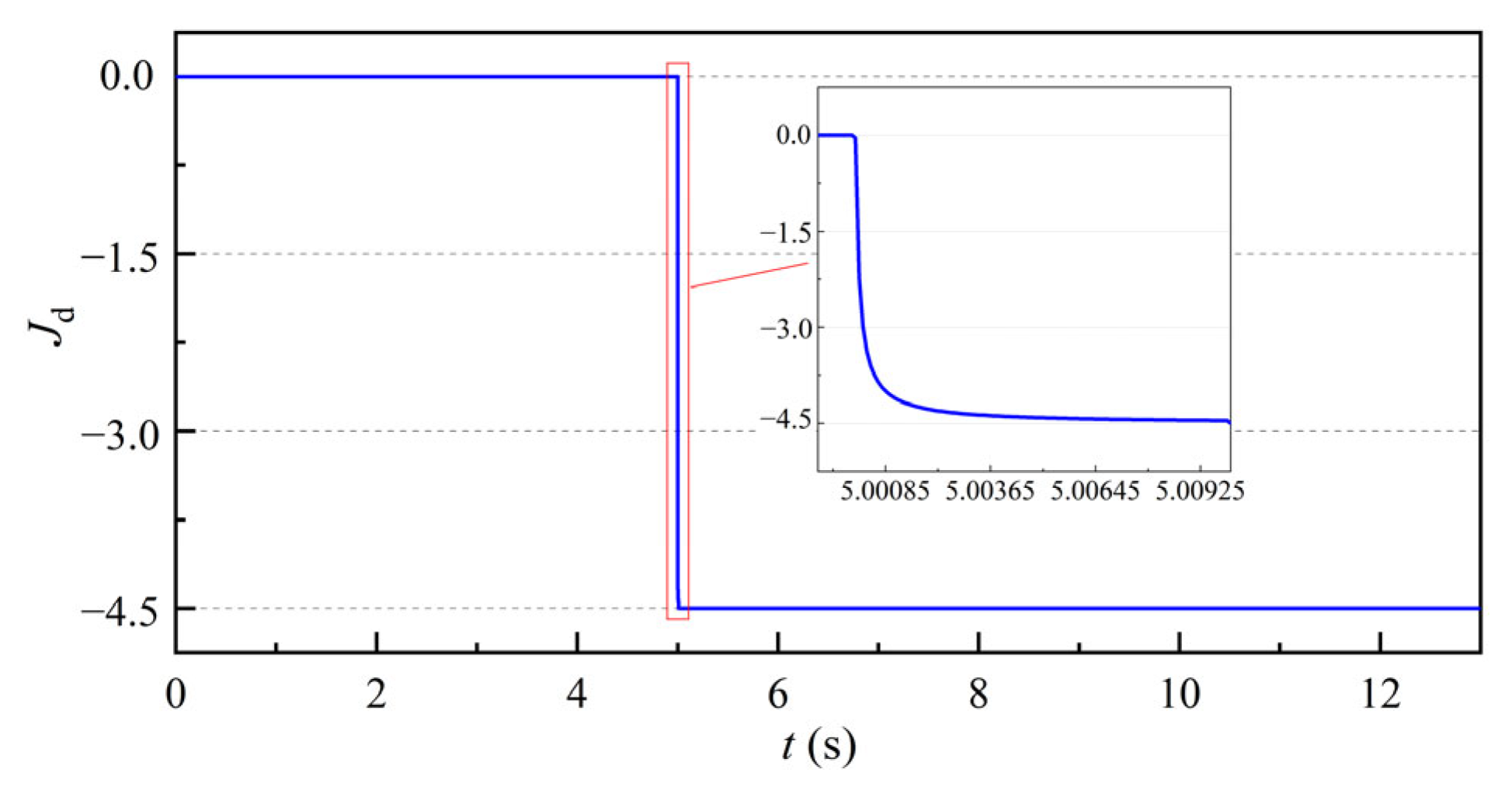
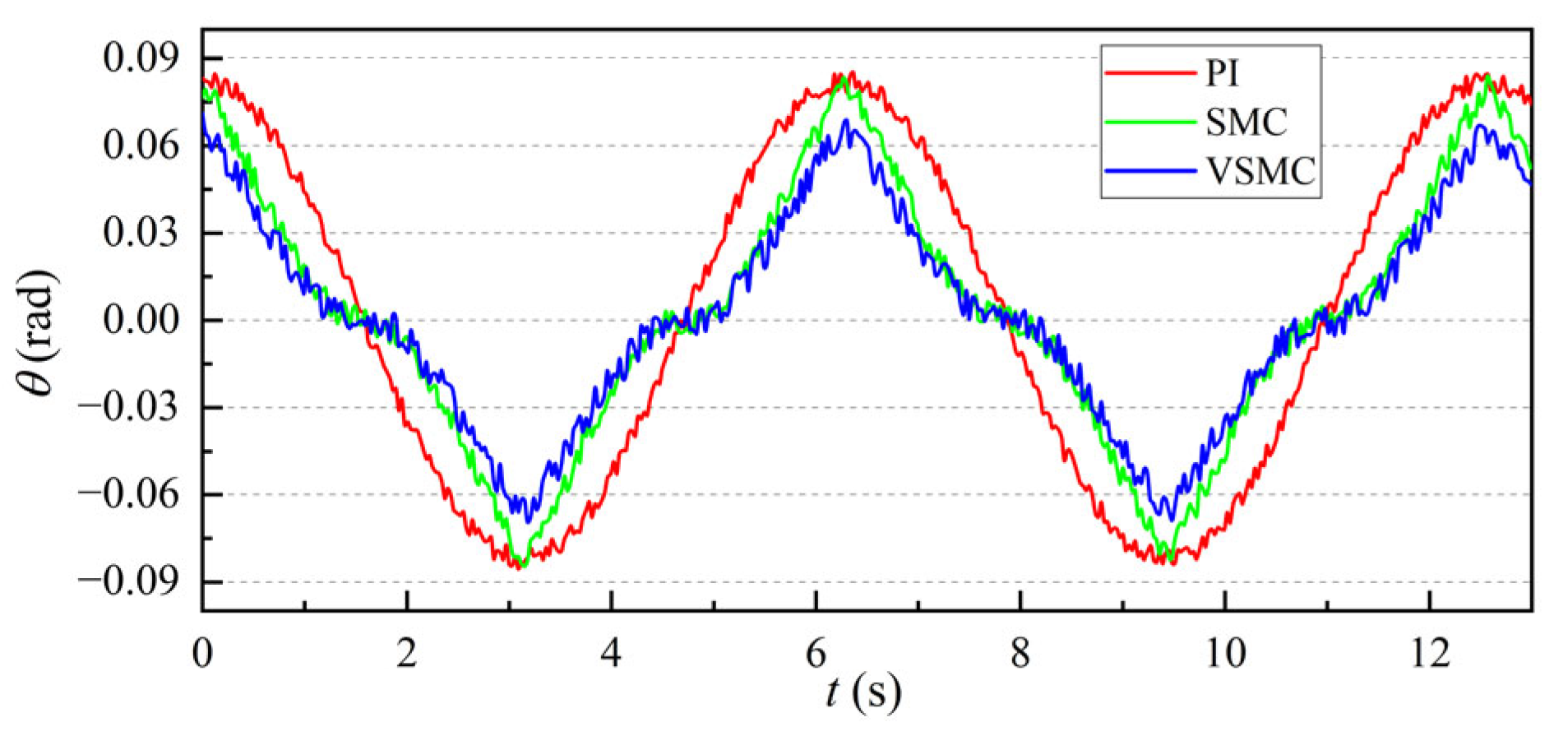
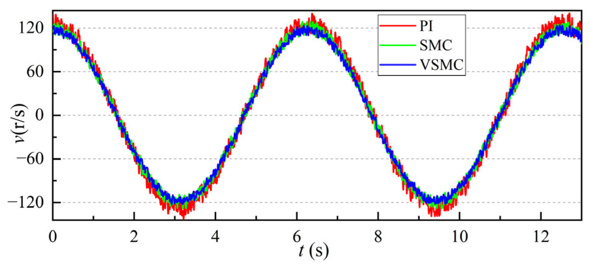
3.1.2. Motor Rotation Response Simulation Analysis

Given the rotational angle as θr = 20 × sin(t) rad/s, the load torque changes from 0 N·m to 4 N·m at 5 s. Figure 8 shows the simulation curves of the rotational angle response for each control method, with an enlarged view demonstrating the motor’s rotational angle response around 5 s. It can be observed from Figure 8 that after adding the load disturbance, the VSMC method exhibits the response that is closest to the reference θr curve compared to the PI and SMC methods.
Figure 9 displays the simulation curves of position response errors for each control method. The initial response error of PI control is approximately 0.18 rad, with a tracking error range from approximately −0.09 to 0.09 rad; the initial response error of SMC is 0.15 rad, with a response error range from approximately −0.075 to 0.075 rad. The initial response error of VSMC is 0.1 rad, with a tracking error range from approximately −0.05 to 0.05 rad. These results show that VSMC reduces both the initial response error and the error range compared to the PI and SMC methods.
Figure 10 shows the disturbance simulation curve, where the observer can rapidly estimate the change in disturbance. From the enlarged view, it can be observed that the response time of the observer to the load change at 5 s is 0.0085 s.
Given the rotational angle as θr = 20×sint rad, as shown in Figure 11, the load torque changes from 0.5 N·m to 1 N·m at 10 s. The motor’s position response, shown in Figure 12, indicates that the initial tracking error of PI control is approximately 0.08 rad, with a response error range from approximately −0.08 to 0.08 rad. The initial response error of SMC is 0.075 rad, with a response error range from approximately −0.08 to 0.08 rad. The initial response error of VSMC is 0.07 rad, with a response error range from approximately −0.07 to 0.07 rad. Adopting the VSMC strategy yields a more accurate rotational response precision and stronger disturbance rejection capability. Figure 13 depicts the angle response curve, indicating that after the load increases, the speed curve of the control strategy proposed in this paper is smoother. Figure 14 illustrates the timely estimation of load changes using the variable-parameter sliding mode control strategy based on the recursive least squares observer when the load changes. Comparing Figure 7, Figure 8 and Figure 9, it can be seen that the experimental results are consistent with the simulation results, which proves the feasibility of the proposed MTPA-ESO control strategy.

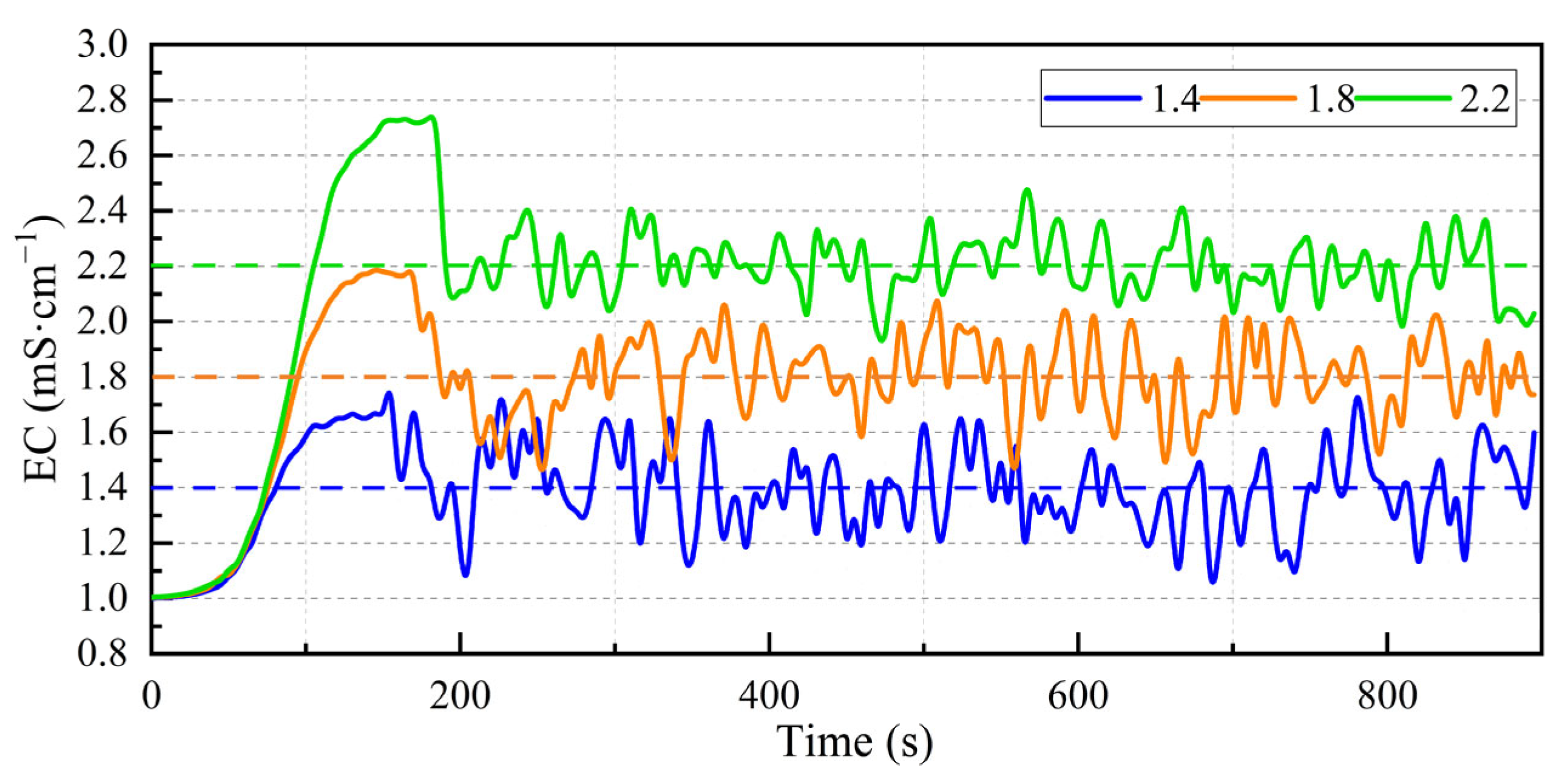
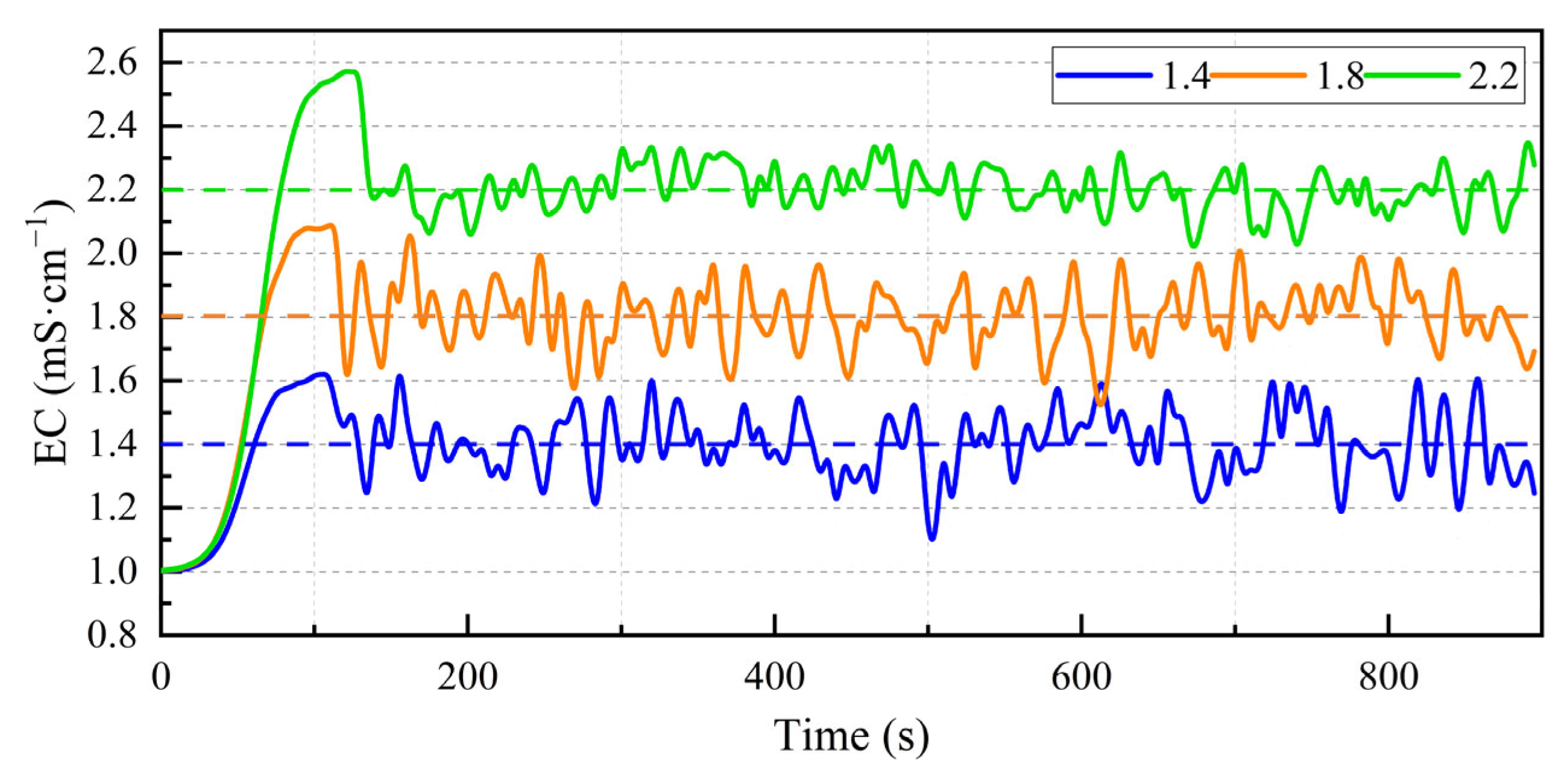
3.2. Experimental Validation

To test the control performance of various methods for remote conductivity control in a water and fertilizer integration machine, a potassium nitrate fertilizer solution was used. The testing device was positioned approximately 110 m from the field sensor section, with sensor sampling every 5 s, resulting in 180 sampling points over a total of 15 min. The EC target values were set at 1.4 mS/cm, 1.8 mS/cm, and 2.2 mS/cm in three separate groups. The control algorithms tested were PI, SMC, and VSMC. The initial EC value was approximately 1.0 mS/cm. Statistical analysis was performed using MATLAB to calculate steady-state EC ranges, settling times, and overshoot.
The comprehensive experimental data (Table 2) shows that in terms of remote conductivity control in water and fertilizer integration systems, the VSMC method performed the best. At a target electrical conductivity (EC) of 1.4 mS/cm, it achieved the smallest EC fluctuation range (0.204 mS/cm), shortest steady-state time (95 s), and lowest overshoot (14.3%). The SMC method exhibited an intermediate performance, with better results than PI but not as good as VSMC. For example, at a target EC of 1.4 mS/cm, the SMC method achieved an EC fluctuation range of 0.181 mS/cm, a steady-state time of 130 s, and an overshoot of 15.6%. These results suggest that SMC offers a balanced trade-off between the higher steady-state time and larger fluctuation observed with PI and the better performance seen with VSMC. In contrast, the PI control method performed the worst, exhibiting the largest EC fluctuation range (0.543 mS/cm), longest steady-state time (190 s), and highest overshoot (25.1%) at a target EC of 2.2 mS/cm.
The experimental results of the control performance for the PI, SMC, and VSMC methods are shown in Figure 15, Figure 16 and Figure 17, respectively.
The PI control method demonstrated a varied performance across different target EC values. For a target EC of 1.4 mS/cm, the system achieved a steady-state EC range from 1.25 to 1.56 mS/cm, with a steady-state time of 160 s and an overshoot of 19.3%. When the target EC was set to 1.8 mS/cm, the steady-state EC ranged from 1.65 to 1.93 mS/cm, the steady-state time increased to 175 s, and the overshoot was 22.2%. At the highest target EC of 2.2 mS/cm, the steady-state EC varied from 2.10 to 2.30 mS/cm, with a steady-state time of 190 s and an overshoot of 25.1%.
The SMC method showed an improved performance compared to the PI control method. For a target EC of 1.4 mS/cm, the steady-state EC ranged from 1.30 to 1.50 mS/cm, with a steady-state time of 130 s and an overshoot of 15.6%. When the target EC was 1.8 mS/cm, the steady-state EC ranged from 1.67 to 1.90 mS/cm, with a reduced steady-state time of 120 s and an overshoot of 16.7%. At the highest target EC of 2.2 mS/cm, the steady-state EC ranged from 2.12 to 2.28 mS/cm, the steady-state time was 130 s, and the overshoot was 17.2%.
The VSMC method demonstrated the best overall performance among the three control algorithms. At a target EC of 1.4 mS/cm, the system reached a steady-state EC range from 1.18 to 1.60 mS/cm, with a steady-state time of 95 s and an overshoot of 14.3%. For a target EC of 1.8 mS/cm, the steady-state EC varied from 1.60 to 1.98 mS/cm, with a steady-state time of 100 s and an overshoot of 15.5%. At the highest target EC of 2.2 mS/cm, the steady-state EC ranged from 2.06 to 2.35 mS/cm, with a steady-state time of 120 s and an overshoot of 16.1%.
Analyzing the results, it is evident that the VSMC method outperformed both the PI and SMC methods in terms of response speed, steady-state time, and overshoot across all tested target EC values. The improved performance of the VSMC method can be attributed to its ability to dynamically adjust the sliding mode surface parameters based on observed values of rotational inertia and load torque. This adaptive capability allows the VSMC method to handle disturbances and changes in system parameters more effectively, leading to more accurate and stable control.
The field experiments further validate these findings, demonstrating that the VSMC method consistently achieved faster steady-state times, lower overshoot percentages, and smaller EC fluctuation ranges. This enhanced performance is particularly significant for practical agricultural applications, where the precise and stable control of water and fertilizer integration is crucial for optimizing crop yields and conserving resources.
The superior performance of the VSMC method highlights its potential as a robust and efficient solution for managing the dynamic and nonlinear characteristics inherent in water and fertilizer integration systems. Its ability to achieve rapid convergence to set points, minimal overshoot, and effective disturbance rejection makes it an ideal choice for improving the efficiency and effectiveness of agricultural irrigation and fertilization processes.
To further validate the effectiveness of the VSMC method in regional irrigation applications, a comparative experiment was conducted between the conventional PI control method and the proposed VSMC-based remote conductivity method. The experiments were performed on the same plot, with a one-month interval between two operations. To minimize external disturbances, artificial irrigation and natural rainfall were avoided for three days prior to each trial. The experimental field was divided into 45 subplots, labeled using a combination of letters (A–E) and numbers (1–9). The deviations between the target and actual applied potassium nitrate fertilizer content across different regions were analyzed (as shown in Figure 18).
The distribution of soil potassium nitrate fertilizer content before and after irrigation was compared to assess the performance of both methods in controlling irrigation uniformity. As illustrated in Figure 5, Figure 6, Figure 7, Figure 8, Figure 9, Figure 10, Figure 11, Figure 12, Figure 13, Figure 14, Figure 15, Figure 16, Figure 17 and Figure 18a, the conventional PI control method exhibited the largest over-application in subplot B8, where 7.48 kg/ha of excess potassium nitrate was applied. The most under-applied region was B2, with a deficit of 6.52 kg/ha. The overall standard deviation of the PI control method was 2.14. In contrast, as shown in Figure 5, Figure 6, Figure 7, Figure 8, Figure 9, Figure 10, Figure 11, Figure 12, Figure 13, Figure 14, Figure 15, Figure 16, Figure 17 and Figure 18b, the VSMC method exhibited a significantly improved uniformity. The largest over-application occurred in subplot C4, with an excess of 1.06 kg/ha, while the most under-applied region was A4, with a deficit of 2.01 kg/ha. The overall standard deviation of the VSMC method was reduced to 0.59, demonstrating its superior precision in achieving the desired fertilizer distribution.

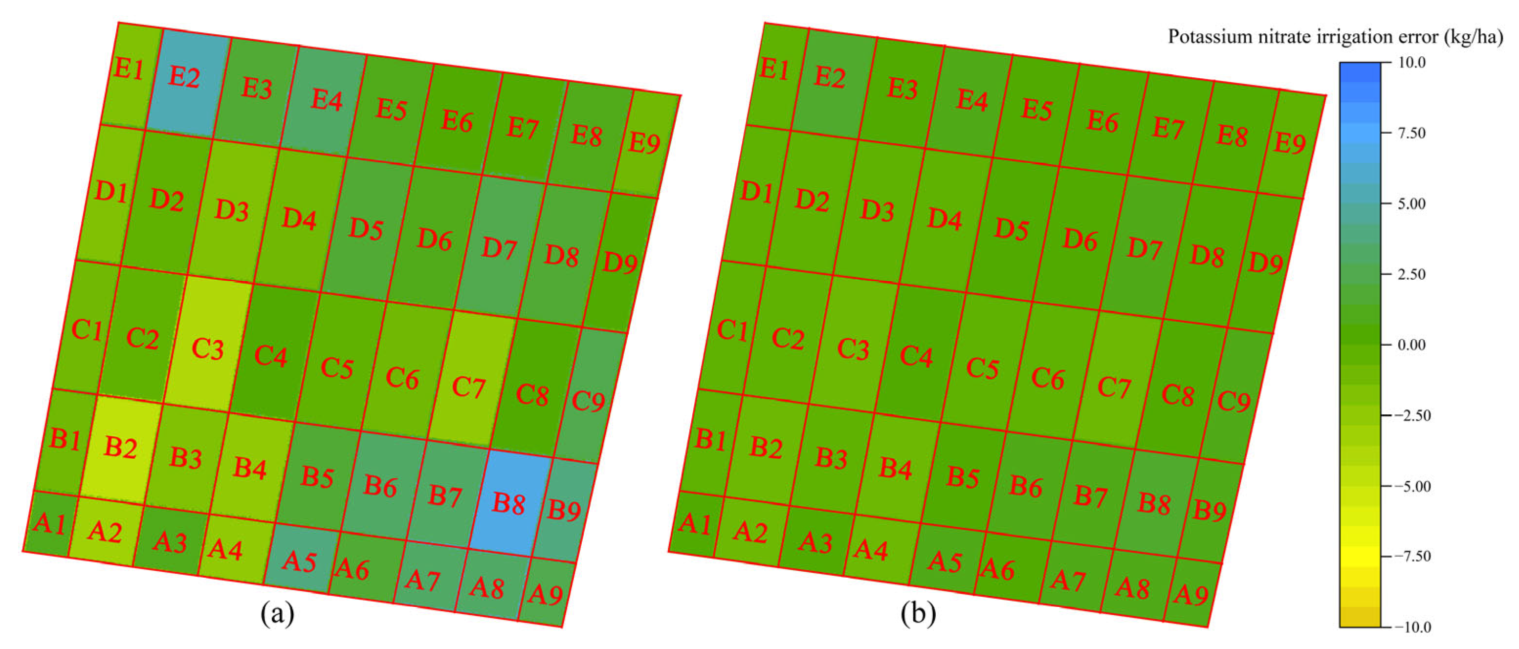
3.3. Field Performance and Adaptive Control Challenges

The experimental and simulation results demonstrate the superiority of the proposed VSMC method with RLS-based adaptive estimation over PI and conventional SMC in terms of response speed, steady-state accuracy, and robustness to load disturbances. However, several practical limitations and uncertainties should be acknowledged.
The control performance relies on the accuracy of the system model, particularly the relationship between motor dynamics and fertilizer flow. While the RLS observer effectively estimates inertia and load torque, unmodeled nonlinearities (e.g., hydraulic resistance, pump wear, or sensor drift) may degrade performance over time. Future work could integrate hybrid modeling (e.g., physics-based and data-driven) to improve adaptability.
The RLS algorithm assumes quasi-static parameter variations, making it less effective under highly dynamic conditions (e.g., sudden pipe blockages or rapid EC fluctuations). In such cases, the observer’s convergence time (0.0085 s in simulations) may lag behind real-world disturbances. Combining RLS with robust filtering (e.g., Kalman or H∞) could mitigate this issue.
The experiments were conducted under controlled disturbances (step torque changes), but actual field conditions involve stochastic factors (e.g., soil heterogeneity and varying water pressure). While VSMC reduced potassium nitrate deviation (SD: 0.59 vs. PI’s 2.14), long-term validation across diverse terrains is needed.
VSMC’s adaptive gains improve responsiveness but may amplify noise in low-signal environments (e.g., noisy EC sensors). A sensitivity analysis of observer tuning parameters (forgetting factor and covariance matrix) would help to balance robustness and noise immunity.
Despite these limitations, the VSMC method significantly advances precision in water–fertilizer integration by dynamically adjusting to operational changes. Its real-time adaptability makes it a promising solution for sustainable agriculture, though further field trials are recommended to refine robustness under extreme conditions.

4. Conclusions

This study developed and validated a variable-structure model control (VSMC) method for water and fertilizer integration systems, effectively addressing nonlinear remote conductivity disturbances and system parameter variability. By incorporating a recursive least squares observer, the proposed system dynamically adjusts electrical conductivity (EC) control, significantly improving the precision of irrigation and fertilization processes.
Simulations revealed that VSMC outperformed the conventional PI and standard SMC methods in response speed, settling time, and disturbance rejection. In step response tests, VSMC achieved the target EC in 0.07 s, compared to 0.14 and 0.12 s for PI and SMC, respectively. VSMC also showed a higher tracking accuracy and better robustness under variable load conditions, markedly reducing steady-state errors.
Field experiments further confirmed these findings. When tested at target EC values of 1.4, 1.8, and 2.2 mS/cm, VSMC consistently achieved more stable and accurate EC regulation than PI and SMC. Regional irrigation trials demonstrated that VSMC significantly improved fertilizer distribution uniformity, lowering the standard deviation of EC from 2.14 (PI control) to 0.59. This mitigated fertilizer over- and under-application across subplots, supporting more sustainable crop management.
Regarding practical implementation, large-scale deployment of the VSMC system requires several prerequisites, as follows: (1) integration with high-precision EC sensors and stable actuator systems, (2) real-time communication infrastructure for feedback control, and (3) adaptive parameter tuning tools for varying soil and environmental conditions. Furthermore, the modularization of control units and compatibility with existing irrigation infrastructure will be key to scalability.
Beyond demonstrating a superior control performance, this research offers valuable insights for designing advanced adaptive control strategies in precision agriculture. Future studies will focus on multi-zone irrigation applications, real-time soil moisture integration, energy optimization, and the application of machine learning to enhance sliding surface parameter adaptation.
In conclusion, the VSMC approach will significantly enhance EC regulation in integrated water and fertilizer systems. It presents a scalable and adaptive solution with a high potential for real-world agricultural deployment, aiming to improve crop productivity, optimize input usage, and reduce environmental footprint.

Author Contributions

Conceptualization, P.Z. and L.Z.; methodology, P.Z.; software, L.Z.; validation, P.Z., Z.L., and L.Z.; formal analysis, L.Z. and X.H.; investigation, L.Z. and X.H.; resources, L.Z. and X.H.; data curation, P.Z.; writing—original draft preparation, P.Z. and L.Z.; writing—review and editing, P.Z. and L.Z.; visualization, P.Z.; supervision, P.Z.; project administration, L.Z.; funding acquisition, L.Z. and X.H. All authors have read and agreed to the published version of the manuscript.

Funding

This research was funded by the Major Science and Technology Special Project of Xinjiang Uygur Autonomous Region, No. 2022A02012-4. This research was funded also by the Corps Science and Technology Plan Project, No. 2023AB005. This research was funded also by the XPCC Science and Technology Plan Project, No. 2022BC004.

Informed Consent Statement

Not applicable.

Data Availability Statement

All relevant data presented in the article are stored according to institutional requirements and, as such, are not available online. However, all data used in this manuscript can be made available upon request to the authors.

Conflicts of Interest

The authors declare no conflicts of interest.

References

  1. Liao, Q.; Nie, J.; Yin, H.; Luo, Y.; Shu, C.; Cheng, Q.; Fu, H.; Li, B.; Li, L.; Sun, Y.; et al. Can the Integration of Water and Fertilizer Promote the Sustainable Development of Rice Production in China? Agriculture 2024, 14, 585. [Google Scholar] [CrossRef]
  2. Souto, A.; Carriquiry, M.; Rosas, F. An integrated assessment model of the impacts of agricultural intensification: Trade-offs between economic benefits and water quality under uncertainty. Aust. J. Agric. Resour. Econ. 2024, 68, 315–334. [Google Scholar] [CrossRef]
  3. Zhong, T.; Zhang, J.; Du, L.; Ding, L.; Zhang, R.; Liu, X.; Ren, F.; Yin, M.; Yang, R.; Tian, P.; et al. Comprehensive evaluation of the water-fertilizer coupling effects on pumpkin under different irrigation volumes. Front. Plant Sci. 2024, 15, 1386109. [Google Scholar] [CrossRef] [PubMed]
  4. Glaser, D.R.; Barrowes, B.E.; Shubitidze, F.; Slater, L.D. Laboratory investigation of high-frequency electromagnetic induction measurements for macro-scale relaxation signatures. Geophys. J. Int. 2023, 235, 1274–1291. [Google Scholar] [CrossRef]
  5. Liu, D.; Li, W.; Gao, H.; Huang, C.; Xu, S.; Liu, W. Organic Water-Soluble Fertilizers Enhance Pesticide Degradation: Towards Reduced Residues. J. Agric. Sci. 2024, 30, 179–192. [Google Scholar]
  6. Kang, Z.J.; Sun, Y.S.; Liu, J.X. An Integrated Parameter Identification Method of Asynchronous Motor Combined with Adaptive Load Characteristics. J. Electr. Eng. Technol. 2023, 18, 1041–1051. [Google Scholar] [CrossRef]
  7. Gan, H.; Cao, Z.; Chen, P.; Luo, Y.; Luo, X. Fractional-order electromagnetic modeling and identification for PMSM servo system. ISA Trans. 2024, 147, 527–539. [Google Scholar] [CrossRef]
  8. Sun, S.; Zhen, S.; Liu, X.; Zhong, H.; Chen, Y.H. Model-based robust servo control for permanent magnet synchronous motor with inequality constraint. Meas. Sci. Technol. 2024, 35, 017002. [Google Scholar] [CrossRef]
  9. Kökçam, E.; Tan, N.S. Comparison of Adaptation Mechanisms on MRAC. IEEE Access 2024, 12, 31862–31874. [Google Scholar] [CrossRef]
  10. Wang, H.; Zhang, L.; Zhao, J.; Hu, X.; Ma, X. Application of Hyperspectral Technology Combined with Genetic Algorithm to Optimize Convolution Long- and Short-Memory Hybrid Neural Network Model in Soil Moisture and Organic Matter. Appl. Sci. 2022, 12, 10333. [Google Scholar] [CrossRef]
  11. Zuo, Y.; Zhu, S.; Cui, Y.; Liu, C.; Lin, X. Adaptive PI Controller for Speed Control of Electric Drives Based on Model Reference Adaptive Identification. Electronics 2024, 13, 1067. [Google Scholar] [CrossRef]
  12. Moreno, J.C.; González, J.; Navarro, A.; Guzmán, J.L. New Tuning Rules of PI+CI Controllers for First-Order Systems. Actuators 2024, 13, 67. [Google Scholar] [CrossRef]
  13. Ji, Y.; Ma, J.; Zhou, Z.; Li, J.; Song, L. Dynamic Yarn-Tension Detection Using Machine Vision Combined with a Tension Observer. Sensors 2023, 23, 3800. [Google Scholar] [CrossRef]
  14. Maraveas, C.; Karavas, C.-S.; Loukatos, D.; Bartzanas, T.; Arvanitis, K.G.; Symeonaki, E. Agricultural Greenhouses: Resource Management Technologies and Perspectives for Zero Greenhouse Gas Emissions. Agriculture 2023, 13, 1464. [Google Scholar] [CrossRef]
  15. Yao, G.; Wang, X.; Wang, Z.; Xiao, Y. Senseless Control of Permanent Magnet Synchronous Motors Based on New Fuzzy Adaptive Sliding Mode Observer. Electronics 2023, 12, 3266. [Google Scholar] [CrossRef]
  16. Li, S.; Li, H.; Wang, H.; Yang, C.; Gui, J.; Fu, R. Sliding Mode Active Disturbance Rejection Control of Permanent Magnet Synchronous Motor Based on Improved Genetic Algorithm. Actuators 2023, 12, 209. [Google Scholar] [CrossRef]
  17. Ahn, Y.-S.; Kim, J.-Y.; Song, K.-Y.; Cho, K.-Y.; Kim, H.-W. Slip prevention algorithm for dual-rotor PM synchronous motor. J. Power Electron. 2024, 24, 382–390. [Google Scholar] [CrossRef]
  18. Ali, K.; Cao, Z.; Rsetam, K.; Man, Z. Practical Adaptive Fast Terminal Sliding Mode Control for Servo Motors. Actuators 2023, 12, 433. [Google Scholar] [CrossRef]
  19. Fadiji, A.E.; Yadav, A.N.; Santoyo, G.; Babalola, O.O. Understanding the plant-microbe interactions in environments exposed to abiotic stresses: An overview. Microbiol. Res. 2023, 271, 127368. [Google Scholar] [CrossRef]
  20. Truong, H.V.A.; Nam, S.; Kim, S.; Kim, Y.; Chung, W.K. Backstepping-Sliding-Mode-Based Neural Network Control for Electro-Hydraulic Actuator Subject to Completely Unknown System Dynamics. IEEE Trans. Autom. Sci. Eng. 2024, 21, 6202–6216. [Google Scholar] [CrossRef]
  21. Xu, H.; Zhou, S.-Z.; Li, X.; Chen, H.; Hu, S. Fast Transient Modulation of a Dual-Bridge Series Resonant Converter. In Proceedings of the IECON 2021—47th Annual Conference of the IEEE Industrial Electronics Society, Toronto, ON, Canada, 13–16 October 2021. [Google Scholar]
  22. Xu, B.L.; Zhang, X.H.; Liu, S.Y. Design method of improved non-singulars terminal sliding mode control systems. In Proceedings of the 2007 Chinese Control and Decision Conference; Northeastern University Press: Shenyang, China, 2007. [Google Scholar]
  23. Nippatla, V.R.; Mandava, S. Comparative vector control study on speed of PMSM drive using sensorless and machine learning techniques: Review. J. Intell. Fuzzy Syst. 2024, 46, 4381–4395. [Google Scholar] [CrossRef]
  24. Rodriguez, J.; Mesny, L.; Chesné, S. Sliding Mode Control for Hybrid Mass Dampers: Experimental analysis on robustness. J. Sound Vib. 2024, 575, 118241. [Google Scholar] [CrossRef]
  25. Zhang, X.; Mao, J.; Zhao, F.; Wang, W.; Jia, R. Speed-current composite loop SPMSM control based on ADR-SMC. IEICE Electron. Express 2024, 21, 20240088. [Google Scholar] [CrossRef]
  26. Su, G.; Guo, Y.; Wang, P.; Cheng, G.; Zhao, D. Research on Control Method of the Power System of Stepping-Type Anchoring Equipment. Sensors 2021, 21, 7123. [Google Scholar] [CrossRef]
  27. Chen, D.H.; Zhang, J.X.; Zhang, T. Sliding mode sensorless control of wind turbine pitch motor with ESO feedforward compensation in the offshore wind power system. Sci. Technol. Energy Transit. 2024, 79, 20. [Google Scholar] [CrossRef]
  28. Wang, H.; Zhao, J.; Zhang, L.; Yu, S. Application of Disturbance Observer-Based Fast Terminal Sliding Mode Control for Asynchronous Motors in Remote Electrical Conductivity Control of Fertigation Systems. Agriculture 2024, 14, 168. [Google Scholar] [CrossRef]
  29. Xu, L.M.; Tippur, H.V.; Rousseau, C.E. Measurement of contact stresses using real-time shearing interferometry. Opt. Eng. 1999, 38, 1932–1937. [Google Scholar] [CrossRef]
  30. Jonker, J.; Doorenbos, C.S.E.; Kremer, D.; Gore, E.J.; Niesters, H.G.M.; van Leer-Buter, C.; Bourgeois, P.; Connelly, M.A.; Dullaart, R.P.F.; Berger, S.P.; et al. High-Density Lipoprotein Particles and Torque Teno Virus in Stable Outpatient Kidney Transplant Recipients. Viruses 2024, 16, 143. [Google Scholar] [CrossRef]
  31. Zhu, F.; Zhang, L.; Hu, X.; Zhao, J.; Meng, Z.; Zheng, Y. Research and Design of Hybrid Optimized Backpropagation (BP) Neural Network PID Algorithm for Integrated Water and Fertilizer Precision Fertilization Control System for Field Crops. Agronomy 2023, 13, 1423. [Google Scholar] [CrossRef]
  32. Huang, A.; Chen, Z.; Wang, J. Research on the dq-Axis Current Reaction Time of an Interior Permanent Magnet Synchronous Motor for Electric Vehicle. World Electr. Veh. J. 2023, 14, 196. [Google Scholar] [CrossRef]
Figure 1. The remote conductivity control system of the fertigation machine.
Applsci 15 04993 g001
Figure 2. Implementation diagram of remote conductivity control system for integrated water and fertilizer machine (APP: mobile application and PLC: programmable logic controller).
Applsci 15 04993 g002
Figure 3. The closed-loop control system diagram. (SPMSM: surface permanent magnet synchronous motor). Note: id and iq* denote the reference (command) values for d-axis and q-axis currents, generated by outer-loop controllers (e.g., speed loop), to regulate motor torque and field orientation.
Applsci 15 04993 g003
Figure 4. Sliding mode control schematic diagram.
Applsci 15 04993 g004
Figure 5. Rotation speed change trend diagram during the position response process.
Applsci 15 04993 g005
Figure 6. The relationship surface between c, TL, and θini.
Applsci 15 04993 g006
Figure 7. Simulation curve of step position response speed for each control method.
Applsci 15 04993 g007
Figure 8. Rotation response simulation curves for each control method.
Applsci 15 04993 g008
Figure 9. Rotation response error simulation curves for each control method.
Applsci 15 04993 g009
Figure 10. Disturbance simulation curve.
Applsci 15 04993 g010
Figure 11. Given angle curve.
Applsci 15 04993 g011
Figure 12. Rotation angle error simulation curves for each control method.
Applsci 15 04993 g012
Figure 13. Speed response simulation curves of each control method.
Applsci 15 04993 g013
Figure 14. The variable-parameter sliding mode control (VSMC) strategy estimates the load simulation curve in time when the load changes.
Applsci 15 04993 g014
Figure 15. The control performance of the Proportional–Integral (PI) control method.
Applsci 15 04993 g015
Figure 16. The control performance of the sliding mode control (SMC) method.
Applsci 15 04993 g016
Figure 17. The control performance of the variable-parameter sliding mode control (VSMC) method.
Applsci 15 04993 g017
Figure 18. Compares the potassium nitrate fertilizer distribution deviation between the Proportional–Integral (PI) control method and the variable-parameter sliding mode control (VSMC) method: (a) PI control method and (b) VSMC method.
Applsci 15 04993 g018
Table 1. Relationship between parameter c and load T.
TL/Nmc
J = 1.75 × 10⁻⁵ kg·m2J = 2.85 × 10⁻⁵ kg·m2
0242198
0.01255206
0.02268212
0.03282222
0.04286232
0.05305240
0.06318249
Table 2. Performance metrics of control algorithms for EC regulation.
Control AlgorithmSet EC
(mS/cm)
Steady-State EC (mS/cm)Steady-State Time (s)Overshoot (%)
PI1.41.25~1.5616019.3
1.81.65~1.9317522.2
2.22.10~2.3019025.1
SMC1.41.30~1.5013015.6
1.81.67~1.9012016.7
2.22.12~2.2813017.2
VSMC1.41.18~1.609514.3
1.81.60~1.9810015.5
2.22.06~2.3512016.1
Disclaimer/Publisher’s Note: The statements, opinions and data contained in all publications are solely those of the individual author(s) and contributor(s) and not of MDPI and/or the editor(s). MDPI and/or the editor(s) disclaim responsibility for any injury to people or property resulting from any ideas, methods, instructions or products referred to in the content.

