Abstract
Flower collection constitutes a critical segment of the flower logistics chain, and its efficiency significantly influences the industry. However, the energy consumption and carbon emissions that occur in the flower collection process present a great challenge for realizing efficient flower collection. To this end, this study proposes a green vehicle routing planning model that incorporates multiple factors, such as fixed costs, refrigeration costs, transportation costs, and so on, to minimize the total costs under hard time window constraints. Moreover, a Genetic Neighborhood Comprehensive Spider Wasp Algorithm (GN_CSWA) is proposed to find the solution to this problem. The random generation and the nearest neighbor algorithms are employed to construct the initial solution, followed by roulette selection, elite selection, and a best individual retention strategy to refine the population for the next iteration. A crossover operator is applied to facilitate global exploration, while six neighborhood search operators are applied to further enhance the quality of the solution. Moreover, to prevent the algorithm from converging to a local optimum, two mutation operators are introduced to generate new solutions. The effectiveness of the proposed optimizer is validated through extensive experimental results.
1. Introduction
Under general logistics transportation conditions, the damage rate for fresh flowers can reach as high as 30% [1]. Consequently, freshly harvested flowers must be immediately transported to refrigerated warehouses using refrigerated vehicles. This requirement arises due to the delicate nature of flowers, which are highly perishable and sensitive to environmental factors such as temperature and humidity. The use of refrigerated vehicles is therefore crucial to maintaining their quality during transit. Although cold chain logistics can effectively preserve the quality of perishable products such as flowers, it is associated with higher energy consumption and carbon emissions compared to conventional logistics [2]. Therefore, cold chain logistics enterprises need to accelerate their transition to a low-carbon economy while exploring sustainable development pathways [3]. This requires innovations in technology and the optimization of logistics processes to reduce the carbon footprint of these operations. This imposes higher requirements on route planning in cold chain logistics, mandating not only stringent control over total transportation costs but also the effective minimization of carbon emissions.
An increasing number of scholars are incorporating environmental factors, such as carbon emissions, into the study of cold chain vehicle routing planning, thereby giving rise to the concept of green cold chain vehicle routing planning [4,5]. This approach aims to reduce the environmental impact of cold chain logistics while maintaining operational efficiency. Green cold chain vehicle routing planning is a variant of the Vehicle Routing Problem (VRP) [6]. The VRP was first introduced by George Dantzig and John Ramser in 1959 [7] and has since become a widely studied combinatorial optimization problem in the fields of operations research and optimization. Designing optimization models that can be applied in real-world scenarios has long been a key focus for scholars. Similarly, developing highly efficient algorithms has also been a major emphasis. Regarding algorithms, exact algorithms invariably encounter the challenge of exponential complexity, whereas classical heuristic algorithms frequently become trapped in local optima [8]. Consequently, many researchers now prefer to use metaheuristic algorithms to solve the VRP [9,10], as these algorithms not only generate high-quality solutions but also offer faster solution times when dealing with complex and large-scale problems.
The contributions of this study are as follows:
- (1)
- For the flower collection problem, a green cold chain vehicle routing planning model incorporating hard time window constraints was developed. This model considers fixed costs, refrigeration costs, transportation costs, carbon emissions costs, flower damage costs, and time penalty costs. It addresses the practical aspects of flower collection by introducing a new method for calculating refrigeration costs. The model strictly adheres to customer-specified collection times to optimize customer satisfaction.
- (2)
- To address the challenges of complex optimization objectives and extensive solution spaces, a novel Genetic Neighborhood Comprehensive Spider Wasp Algorithm (GN_CSWA) is proposed. The algorithm combines random generation with the nearest neighbor algorithm to generate diverse and high-quality initial solutions. It employs three selection strategies—roulette wheel selection, elite selection, and best individual retention strategy—to select individuals for the next iteration, ensuring that the selected population has good genetic material and sufficient diversity. The initial search is conducted using the Partial Mapping Crossover (PMX) operator. Based on the time–distance matrix and elite chromosome information, two new search operators are designed. Meanwhile, in-route and out-route search operators, as well as two mutation operators, are introduced to conduct further searches.
- (3)
- Through extensive simulation experiments utilizing real-world traffic network data and Solomon benchmark datasets [11], the effectiveness of the proposed model and algorithms was validated. The experimental results demonstrated that the model can significantly reduce total transportation costs and carbon emissions. Additionally, the proposed algorithm demonstrated superior solution quality and convergence speed, yielding more cost-effective delivery path solutions.
The remainder of this paper is structured as follows: Section 2 provides an overview of the advancements in related research; Section 3 presents a detailed problem analysis; Section 4 introduces the proposed solution; Section 5 validates the effectiveness of the proposed model and algorithms through simulation experiments; and Section 6 provides a summary and outlines future work plans.
2. Literature Review
We review previous studies on vehicle routing planning in cold chains for fresh agricultural products, pharmaceuticals, and other relevant areas. Table 1 and Table 2 present a comparative analysis between the work in the existing literature and the approach proposed in this study.

Table 1.
Comparison of solutions from the existing literature with the solution proposed in this paper.

Table 2.
Comparison of models from the existing literature with the model proposed in this paper.
Hou et al. [12] incorporated time window constraints and the spoilage costs of perishable goods into their research, developing an optimization model for fresh food cold chain delivery routes to minimize total costs. They proposed an improved genetic algorithm (GA) to solve this model. Qi et al. [13] extended the application scope of cold chain distribution route planning, particularly in emergency cold chain logistics, and proposed an improved ant colony algorithm to solve these problems. Song et al. [14] conducted research aimed at improving customer satisfaction without increasing energy consumption and proposed an improved artificial fish swarm algorithm to solve this problem. The study differs from previous work in that it focuses on improving customer satisfaction and controlling energy consumption rather than merely minimizing costs. Du et al. [15] considered factors like customer satisfaction, vehicle fuel consumption, refrigeration costs, and cargo damage costs, proposing an improved simulated annealing algorithm with a neighborhood solution generation strategy. Ji et al. [16] proposed a bi-objective optimization model for fruit cold chain distribution aimed at minimizing total costs and maximizing customer satisfaction. They combined genetic algorithms with the acceptance mechanism of simulated annealing and periodically updated the population by randomly selecting one of three neighborhood searches to solve the problem. Wu et al. [17] introduced the concept of time tolerance, establishing an optimization model that balances time tolerance and total costs to meet high customer time requirements. They improved the multi-objective simulated annealing algorithm by combining hybrid stochastic–fixed step sizes with elite strategies to solve the problem. The work highlighted the time sensitivity in cold chain logistics during optimization.
In the following studies, the optimization objectives of cold chain vehicle route planning aimed to minimize total costs while simultaneously reducing carbon emissions. Chen et al. [18] considered factors such as the damage costs of fresh agricultural products and carbon emissions costs, and they proposed an optimization model aimed at minimizing the total costs. They solved it using an improved ant colony algorithm combined with tabu search. The study focused on the issue of carbon emissions. Zhang et al. [19] considered various costs involved in cold chain distribution, including fixed costs, transportation costs, refrigeration costs, damage costs, and carbon emissions costs, establishing a cold chain route optimization model. They proposed a solution that combines ribonucleic acid computation with ant colony optimization (ACO). Ning et al. [20] developed a cold chain distribution model that incorporates transportation, refrigeration, carbon emissions, and time penalties to minimize total costs, solved by an improved quantum ant colony algorithm based on adaptive rotation angles. Yao et al. [21] considered logistics costs in the cold chain distribution of fresh agricultural products from two aspects: carbon tax and preservation investment. They developed a green vehicle routing optimization model for fresh agricultural products aimed at minimizing total costs, which was solved using an improved ant colony algorithm. Fang et al. [22] developed a long-distance cold chain logistics route optimization model that incorporates the damage costs due to distribution vibration and the carbon emissions costs from refrigerants. They proposed an improved ant colony algorithm to solve this model. Compared with previous studies, they paid more attention to the details of the actual transportation process. Shao et al. [23] investigated the optimization model for pharmaceutical cold chain logistics. They improved the Grey Wolf Optimizer by incorporating large neighborhood search (LNS) and utilized a greedy algorithm along with enhanced nonlinear factors to improve convergence speed. Although the study primarily focused on pharmaceutical cold chain distribution, its optimization methods provided a valuable reference for cold chain vehicle routing planning.
Many scholars have conducted in-depth research on cold chain vehicle routing problems, but their focuses differ. Current studies primarily concentrate on vehicle routing for fresh produce distribution under soft time window constraints, with less attention given to vehicle routing for flower collection under hard time window constraints. Some studies consider only one or more of the following factors: customer satisfaction, transportation costs, and carbon emissions costs. It is observed that most research employs improved genetic algorithms or ant colony optimization algorithms to solve these problems. However, the Spider Wasp Optimizer (SWO) has been proven suitable for solving complex optimization problems, and few studies have applied the SWO algorithm to VRP problems. Therefore, this paper integrates existing optimization approaches and targets practical collection scenarios to propose a more comprehensive and efficient low-carbon cold chain routing planning model for flower collection. Furthermore, this paper also designs an improved SWO algorithm to address low-carbon cold chain routing planning problems.
3. Problem Analysis and Mathematical Model
3.1. Problem Description
As shown in Figure 1, a fleet of homogeneous refrigerated vehicles is stationed at a central warehouse and tasked with collecting flowers from various customer-designated locations before returning to the warehouse. The locations of customers, the required flower collection weight at each site, the time windows, and the service durations are all predetermined before vehicle departure. Each flower collection point can be visited by only one vehicle, and the total weight of flowers collected along a vehicle’s route must not exceed its maximum loading capacity.
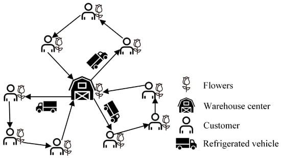
Figure 1.
Vehicle routing model for flower collection.
To define the application scenario of the model, the following assumptions are established:
- (1)
- The number of available vehicles in the warehouse, the maximum load capacity of each vehicle, each vehicle’s speed, and a predefined set of customers with collection locations, required weights, time windows, and service durations are known.
- (2)
- The vehicle consumes fuel and generates carbon emissions while driving. However, during flower collection, the engine is turned off, and there is no fuel consumption or carbon emissions.
- (3)
- The customer’s time window is a hard constraint. The vehicle may arrive earlier than the earliest service time but must wait until the service window opens to collect flowers. If the vehicle arrives later than the latest allowable time, the customer will reject the service.
- (4)
- Only one type of flower needs to be collected, and the collection method, carriage temperature, and other related conditions are all the same.
3.2. Model Parameters
To better represent the green cold chain vehicle routing planning model for flower collection, the parameters and variables as shown in Table 3 and Table 4.

Table 3.
Parameters and variable symbol description table.

Table 4.
Decision variables table.
3.3. Costs Variables Analysis
3.3.1. Fixed Costs
The fixed costs consist of vehicle wear costs and labor costs. Vehicle wear costs refer to the depreciation and maintenance expenses incurred due to the vehicle undergoing wear and tear. Labor costs represent the wages paid to the drivers. Therefore, the total fixed costs can be calculated using Equation (1).
3.3.2. Refrigeration Costs
When collecting flowers, opening the vehicle door allows warm external air to enter, causing a significant change in the internal temperature. This differs from the scenario where the doors remain closed. Consequently, the fuel consumption during the refrigeration process consists of two components: the fuel consumed while the vehicle is driving or possibly waiting with the doors closed, and the fuel consumed when the doors are opened for flower collection. It is important to note that before the vehicle departs from the warehouse and arrives at the first customer for collection, no flowers are onboard requiring refrigeration, and thus no fuel consumption is incurred. The total fuel consumption during the refrigeration process can be calculated using Equation (2).
Therefore, the total refrigeration costs can be calculated using Equation (3), which is expressed as follows:
3.3.3. Transportation Costs
Transportation costs refer to the fuel consumption incurred by the engine while the vehicle is driving. To analyze fuel consumption during vehicle operation, the load estimation method is used to calculate fuel usage while driving [24]. The total engine fuel consumption during the vehicle’s flower collection process can be calculated using Equation (4).
Therefore, the total transportation costs can be calculated using Equation (5).
3.3.4. Costs of Carbon Emissions Associated with Flower Collection
CO2 is produced both when the refrigeration system consumes fuel to maintain low temperatures and when the vehicle is in motion. Therefore, the total carbon emission costs can be calculated using Equation (6).
3.3.5. Costs of Flower Damage
During the flower collection process, opening the vehicle door causes a rise in temperature due to air convection, which exacerbates damage to the flowers. Therefore, the damage coefficient for flowers differs when the vehicle is in motion or waiting to serve a customer with the doors closed compared to when the doors are open during the flower collection process. It is assumed that the flower damage coefficient when the refrigerated vehicle’s door is closed is smaller than when the door is open, with . Vehicle k travels from customer i to customer j, and before it begins serving customer j, the duration for which the door remains closed is given by . The costs of flower damage can be calculated using Equation (7).
3.3.6. Time Penalty Costs
To address solutions generated during the search process that violate time window constraints, the model introduces time penalty costs to improve solution quality through a penalty mechanism. If the vehicle arrives before the earliest time window, it incurs a penalty due to the required waiting time; if the vehicle arrives after the latest time window, it also incurs a penalty. The time penalty costs can be calculated using Equation (8).
3.4. Mathematical Model
Based on the analysis above, the flower collection vehicle routing model, with the objective of minimizing the total cost, can be expressed as follows:
Equation (9) represents the optimization objective function of this paper, which consists of fixed costs, refrigeration costs, transportation costs, carbon emission costs, flower damage costs, and time penalty costs; Equation (10) indicates that each customer can only be visited by one vehicle once; Equation (11) indicates that each vehicle can only be used once; Equation (12) indicates that the vehicle arrives at and leaves from the same customer node; Equation (13) indicates that the total demand of all customers served by a vehicle must not exceed its maximum load capacity; Equation (14) indicates that the vehicle starts from the warehouse, completes the flower collection tasks, and then returns to the warehouse; Equation (15) indicates the constraint that relates the vehicle’s arrival time, waiting time, service time, and departure time; and Equation (16) indicates the relationship between the road segment distance and travel time.
4. Algorithm Design
4.1. Traditional Spider Wasp Optimizer
SWO is a nature-inspired metaheuristic algorithm introduced by Mohamed Abdel-Basset et al. [25] in 2023. The algorithm is inspired by the hunting, nesting, and mating behaviors of female spider wasps in nature. The hunting behavior of female wasps consists of two distinct phases: the search phase and the follow-and-escape phase. SWO has proven to be particularly effective in solving complex optimization problems, especially those characterized by nonlinearity and high dimensionality [26,27,28].
4.2. GN_CSW Algorithm Design
VRP is an NP-hard problem, with a vast solution space [29]. The green cold chain path optimization problem not only requires cost minimization but also needs to consider the reduction of energy consumption and carbon emissions, making the optimization objective more complex [30]. To solve this problem, this paper proposes a new GN_CSWA, which combines the advantages of GA, LNS, and SWO. GA has strong global search capabilities [31], LNS offers higher flexibility [32], while SWO effectively integrates both global and local search strategies [33]. However, SWO is mainly applicable to continuous optimization problems and cannot directly solve discrete problems. To reduce the complexity of SWO and achieve discretization, GN_CSWA makes adjustments to the initial solution generation method and population update strategy rather than directly adopting the original SWO method. Additionally, some parameters from the original SWO are not incorporated. The choice of using SWO is due to its ability to effectively integrate the advantages of both global and local search strategies, particularly in solving complex high-dimensional optimization problems. By combining the strengths of GA, LNS, and SWO, GN_CSWA significantly enhances algorithm performance during the optimization process, making it particularly suitable for solving problems like green cold chain path optimization, which requires efficient exploration of the solution space.
The basic steps of the GN_CSWA are outlined as follows:
- (1)
- Initial solutions that are both diverse and of high quality are generated using a combination of random methods and the nearest neighbor algorithm.
- (2)
- Three selection strategies, including roulette wheel selection, elitism, and best individual retention, are used to select individuals for the next iteration, allowing for the inheritance of high-quality genes while maintaining population diversity.
- (3)
- A global search is performed by utilizing the PMX operation to broaden the search space.
- (4)
- A further localized search of the solution space is performed by carefully balancing the use of six search operators across three phases: the discretized SWO search phase, the discretized SWO follow-and-escape phase, and the discretized SWO nesting behavior phase.
- (5)
- New solutions are generated by applying discrete SWO mating operations and inverse mutation operations, preventing population homogenization and avoiding convergence to local optima.
The flowchart of GN_CSWA is shown in Figure 2, where the parameter represents random number, where . , , , , and are constants. The specific roles of each parameter are shown in Table 5.
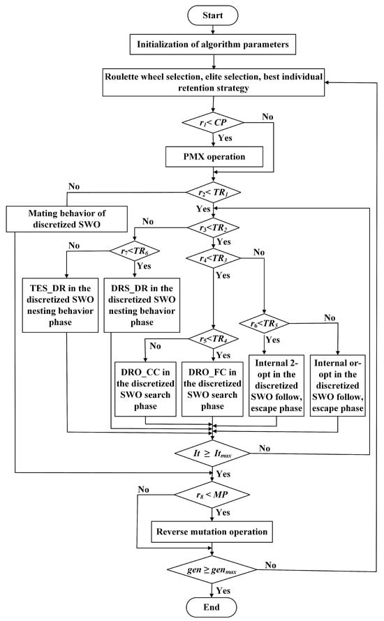
Figure 2.
Flowchart of GN_CSWA.

Table 5.
Algorithm parameters description table.
4.3. Encoding and Decoding
- (1)
- Encoding method: A chromosome is composed of a sequence of integers, where the arrangement of the sequence represents the order in which vehicles visit customers. This encoding method does not contain specific path segmentation information but only describes the overall access order of all customers.
- (2)
- Decoding method: During the decoding process, the integer zero, which represents the warehouse center, is inserted into the customer sequence based on the vehicles’ maximum load capacities and the customers’ time window constraints. This insertion effectively divides the sequence into multiple subroutes, each delimited by two zeros, which represent the sequence of customers served by a single vehicle. When the load of a vehicle exceeds its capacity, a zero is inserted to indicate a new route, and a new vehicle is assigned to continue the deliveries. This ensures that no vehicle exceeds its capacity while respecting the time window constraints for each customer. Each chromosome corresponds to a complete routing plan, and this encoding method guarantees that every chromosome can be successfully decoded into a feasible solution. This process is illustrated in Figure 3.
 Figure 3. Example of chromosome encoding and decoding.
4.4. Generating Initial Solutions
To ensure both the quality and diversity of the initial solutions, random generation and the nearest neighbor algorithm are employed to generate the initial solutions.
- (1)
- Random generation method: A sequence of integers is randomly generated, ensuring no duplicate numbers.
- (2)
- Nearest neighbor algorithm method: First, a customer is randomly selected. Then, the nearest unvisited customer that satisfies both the load and time window constraints is chosen. This process is repeated until all customers have been visited.
4.5. Fitness Function
The derivative of the objective function in the optimization model is used as the fitness function for the algorithm, where a higher fitness value indicates a better solution.
4.6. Select Operation
Before each iteration of GN_CSWA, three selection mechanisms are employed: (1) Roulette wheel selection: This strategy randomly selects 90% of the individuals from the parent generation, minus one. The selection probability of each individual is determined by its fitness value, with higher fitness values increasing the likelihood of being selected for crossover and mutation. (2) Elite selection: The top 10% of individuals with the highest fitness values from the parent generation are directly selected for crossover and mutation. (3) Best individual retention: The individual with the highest fitness value is retained for the next generation without undergoing crossover or mutation.
4.7. Global Search Based on PMX
PMX is a widely used genetic operator in combinatorial optimization, recognized for its ability to preserve partial genetic structures from parent solutions while generating new offspring. In the GN_CSWA, PMX is applied during the global search phase to enhance diversity and improve solution quality. Individuals are paired from the population selected by the three selection mechanisms described in the previous section, and each pair is traversed sequentially. For each pair, if a randomly generated number is less than the predefined crossover probability, the crossover operation is performed to generate new offspring; otherwise, the pair remains unchanged. The process is illustrated in Figure 4 and follows these steps: (1) Two crossover points are randomly selected to determine the crossover interval, and the gene sequence within this interval is mapped to the offspring as a retained fragment. (2) Two offspring individuals are produced by exchanging the retained gene segments between parent 1 and parent 2 within the crossover interval. (3) After exchanging gene segments, duplicate or missing genes may appear. To address this, the offspring must be repaired by correcting any duplicates or omissions, ensuring that each generated offspring is a valid solution.
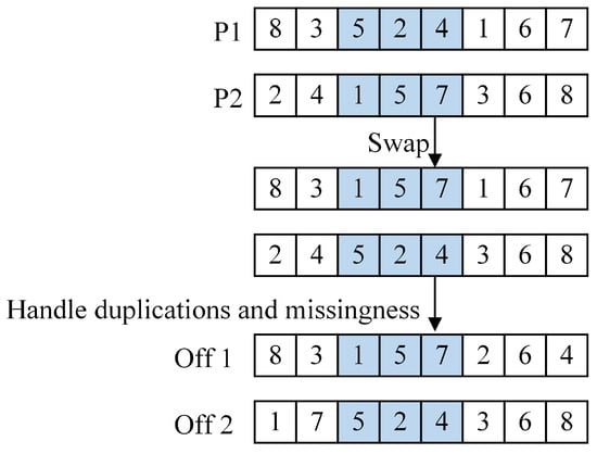
Figure 4.
The PMX procedure.
4.8. Local Search Based on Six Neighborhood Search Operators in Discrete SWO
In the GN_CSWA, local search is performed by making a trade-off between the use of six neighborhood search operators across three phases: the discretized SWO search phase, the discretized SWO follow-and-escape phase, and the discretized SWO nesting behavior phase.
4.8.1. The Discretized SWO Search Phase
When the distance between two customers is short but their time windows differ significantly, serving them consecutively with the same vehicle may lead to increased waiting time. Conversely, if two customers have similar time windows but are geographically far apart, assigning them to the same vehicle may violate the hard time window constraint. Therefore, both temporal and spatial factors should be considered when designing the neighborhood search operator. Additionally, chromosomes with higher fitness values typically contain gene segments similar to those in the optimal solution. Preserving these high-quality gene segments and passing them to the next generation helps propagate superior genes throughout the population, accelerating the algorithm’s convergence.
- (1)
- Damage Repair Operators Based on Frequency of Occurrence and Connectivity Probability(DRO_FC): The top 10% of chromosomes with the highest fitness in the population are selected to form the elite population. The most frequently occurring customers at each position within the chromosomes of the elite population are then counted to construct temporary routes. Customers matching the temporary routes are retained, while the remaining ones are removed. The connection probability between nodes is calculated using the spatio-temporal distance matrix [34] and common information from the elite population. This probability represents the likelihood that two nodes will be visited consecutively by the same vehicle. Deleted customers are then reinserted into the route based on this probability; in this case, a higher connection probability indicates a lower incremental routing cost when reinserting the node. Based on the spatial–temporal distance matrix and the common information of the elite population, the connection probability between nodes i and j can be computed using the following formula:where is the weighting factor in the formula that regulates the balance between spatial-temporal distance and adjacency information of nodes within the elite population. denotes the spatial-temporal distance between nodes i and j, while denotes the total number of times nodes i and j are adjacent in the elite population. The spatial-temporal distance between nodes i and j is determined by the following formula.denotes the weighting factor that balances spatial and temporal distances. denotes the time distance between customers i and j.
- (2)
- Damage Repair Operators Based on Common Subsequence and Connectivity Probability(DRO_CC): The longest common subsequence [35] with the elite individual is retained, and the remaining customers are subsequently removed. The connection probability between each customer is then calculated using the aforementioned Equations (17) and (18), and the removed customers are reinserted into the route based on their connection probabilities.
4.8.2. The Discretized SWO Follow-and-Escape Phase
- (1)
- Internal 2-opt: Two edges within the same route are randomly selected, disconnected, and then reconnected in a different order. If the total costs after reconnection are lower, the exchange is accepted; otherwise, the original configuration is retained. This process is illustrated in Figure 5a.
- (2)
- Internal or-opt: A segment within the same route, consisting of two consecutive nodes, is selected and relocated to a different position within the route. If the total route costs decrease after the relocation, the move is accepted; otherwise, the original configuration is retained. This process is illustrated in Figure 5b.
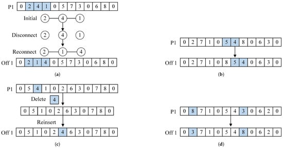
Figure 5.
The four types of search operator procedures: (a) The 2-opt procedure. (b) The or-opt procedure. (c) The deletion and reinsertion procedure outside the route. (d) The swap procedure outside the route.
4.8.3. The Discretized SWO Nesting Behavior Phase
- (1)
- Deletion Reinsertion Search Operator Based on Different Routes (DRS_DR): A randomly selected customer is removed from the current route and inserted into a different route. The operation is executed if the total costs of the newly formed path are lower than that of the original path; otherwise, no changes are made. This process is illustrated in Figure 5c.
- (2)
- Two-Point Exchange Search Operator Based on Different Routes (TES_DR): Two different routes are randomly selected from the path, and a node from each route is swapped. If the total costs of the newly formed path are lower than that of the original path, the swap operation is executed; otherwise, no changes are made. This process is illustrated in Figure 5d.
4.9. Mutation Operators
4.9.1. Discretized SWO Mating Behavior
Based on the research of Qi et al. [36], a temporary set consisting of the three most frequently occurring consecutive customers is constructed based on the elite population. Two parent individuals, parent 1 and parent 2, are randomly selected, and gene segments in the parents that match the temporary set are preserved in offspring 1 and offspring 2. The vacant positions in offspring 1 are filled with nonduplicate genes from parent 2, while those in offspring 2 are filled with nonduplicate genes from parent 1. This process is illustrated in Figure 6. The application of this mutation operation is controlled by the parameters described in Section 4.2.
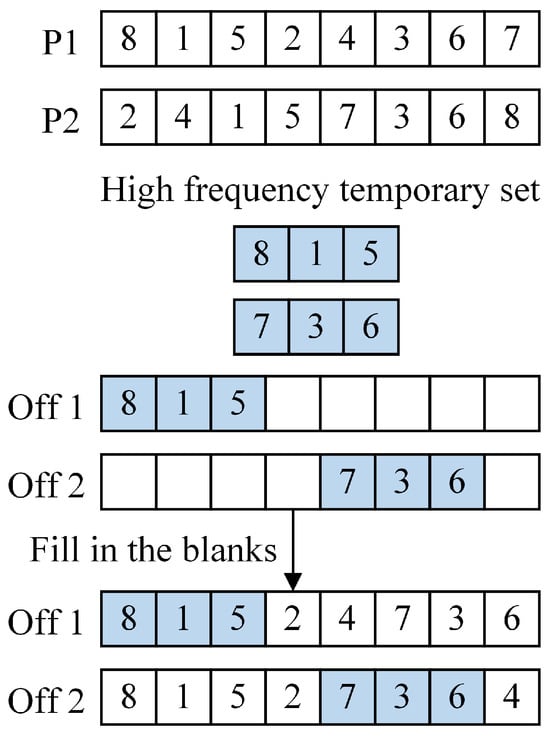
Figure 6.
The discretized SWO mating behavior procedure.
4.9.2. Reverse Mutation
Reverse mutation: Two positions within the path are randomly selected to determine the reverse operation interval, after which the genes within this interval are reversed. This process is illustrated in Figure 7. The application of this mutation operation is controlled by the reverse mutation probability.
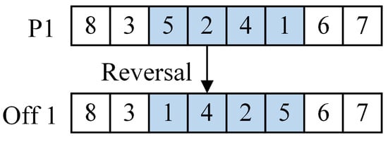
Figure 7.
The reverse mutation procedure.
4.10. Complexity Analysis of the GN_CSW Algorithm
In analyzing the time and space complexity of the GN_CSWA, we consider various steps of the algorithm, including initial solution generation, fitness function calculation, selection operations, PMX operation in the global search phase, six neighborhood search operators in the local search phase, and mutation operations. The complexity analysis for each step is detailed below:
- (1)
- The initial solution generation employs both the random method and the nearest neighbor algorithm. The random method involves simply sorting the customers randomly, so its time complexity is . The nearest neighbor algorithm requires traversing each customer and calculating the distance to the unvisited customers. For each customer, selecting the nearest unvisited customer requires traversing n customers, resulting in a time complexity of . Therefore, the overall time complexity is dominated by the nearest neighbor algorithm, which is . The space complexity is .
- (2)
- The calculation of the fitness function involves summing multiple cost components and performing numerical computations, which require traversing customers or edges. The time complexity is , where is the population size and n is the number of customers. The space complexity is .
- (3)
- The selection operation includes roulette wheel selection, elite selection, and best individual retention strategy. Each selection mechanism requires only a single traversal of the parent population, resulting in a time complexity of and a space complexity of .
- (4)
- The time complexity of the PMX operation in the global search phase is , involving gene exchange and repair. The space complexity for storing the offspring is .
- (5)
- The time complexity of the six search operators involved in the local search is as follows: For DRO_FC, the time complexity for counting the frequency of each gene in the elite population is , and the time complexity for calculating the connection probability is also , resulting in a total time complexity of . Similarly, for DRO_CC, the time complexity for calculating the longest common subsequence and the connection probability are both , leading to a total time complexity of . For the Internal 2-opt operator, which involves selecting two edges and reconnecting them, the time complexity is . The Internal or-opt operator, which functions similarly to the 2-opt operator, also has a time complexity of . Both DRS_DR and TES_DR operators, which involve delete–insert operations and node swapping between two routes, respectively, have time complexities of . Since only one search operator is executed at a time during each local search, the overall time complexity is dominated by DRO_FC and DRO_CC, resulting in a total time complexity of . In terms of space complexity, it is , as it is primarily used for storing paths and intermediate results.
- (6)
- The mutation operations consist of two components: the discretized SWO crossover operation and the reverse mutation operation. The time complexity of the discretized SWO crossover operation is , as it generates offspring by exchanging genes between parent individuals, and the process is linear. The space complexity of this operation is , which is used to store the paths and intermediate results. The time complexity of the reverse mutation operation is , where is the length of the reversal interval, typically at most n, so its time complexity is . The space complexity of this operation is also , used for storing paths and intermediate results.
Based on the above analysis, the time complexity of the GN_CSWA is primarily dominated by the fitness function calculation and the DRO_FC and DRO_CC search operators in the local search phase, with a total time complexity of . The space complexity is mainly used to store paths, individuals, and intermediate results, resulting in a total space complexity of .
5. Numerical Experiments
5.1. Parameter Setting
Drawing upon insights from the existing literature, the parameter values in the model are set as shown in Table 6.

Table 6.
Values of relevant parameters in the model.
The algorithm parameters in this study are set based on the existing literature and experimental results, with reasonable adjustments made according to the specific characteristics of the problem. The following provides a brief discussion of the rationale behind the parameter settings for each algorithm.
GA: The algorithm parameters are primarily based on reference [37], combined with experimental results. The population size is set to 40, and the number of iterations is set to 200. The crossover operator used is PMX, with a crossover probability of 0.85. The mutation operator is the inversion mutation, with a mutation probability of 0.1. A higher crossover probability helps maintain the diversity of the population, while a lower mutation probability introduces randomness while maintaining the stability of the population.
ACO: In this study, the number of ants is set to 50 and the number of iterations is set to 200 based on existing literature and experimental results. These settings ensure that the algorithm can thoroughly explore the solution space within a reasonable computation time. The pheromone evaporation rate is set to 0.1, and the importance coefficient of the heuristic information is set to 2 to balance exploration and exploitation. The initial pheromone level is set to the reciprocal of the objective function value of the initial solution, ensuring that the algorithm can obtain reasonable heuristic information in the early stages.
Hybrid Simulated Annealing and Tempering Algorithm (HSATA): The parameters of this algorithm are set based on reference [38]. The initial temperature is set to 1000, and the termination temperature is set to 0.05. The number of iterations at each temperature is set to 250, and the cooling rate is set to 0.95. The probabilities for the exchange operator, inversion operator, and insertion operator are 0.2, 0.5, and 0.3, respectively. The iteration termination count is set to 1500. A higher initial temperature and a moderate cooling rate help the algorithm perform an extensive search in the early stages and make fine adjustments as it approaches convergence.
Genetic Algorithm Combined with Grey Wolf Optimizer (GA_GWO): Based on the existing literature and experimental results, the population size of the algorithm is set to 40, and the number of iterations is set to 200. The global search follows the settings of the aforementioned GA, while the local search is implemented using the improved Grey Wolf Optimizer combined with the LNS algorithm. The LNS algorithm utilizes a combination of random deletion and greedy insertion operators, which effectively explore the solution space while maintaining the quality of the solutions.
GN_CSWA: The parameters of this algorithm are set based on the existing literature and experimental experience, fully considering the limitations of computational resources and the adaptability to problem scale. The population size is set to 10, and the number of iterations is set to 200. The PMX crossover probability () is 0.85, and the inversion mutation probability () is 0.1. To further enhance the algorithm’s search capability, the local search parameters were fine-tuned through experiments, with reasonable parameters selected. The specific parameter settings are as follows: = 0.95, = 0.8, = 0.85, = 0.8, = 0.5, = 0.5, = 6.
5.2. Basic Data
This study uses two types of benchmark datasets. The first type is from the Solomon dataset, which includes three instances: R101, C101, and RC101. Each instance contains 100 customers and one warehouse center. In R101, the customer locations are randomly distributed; in C101, the customer locations are clustered; and RC101 is a combination of random and clustered distributions. The second type of dataset is generated based on real map data. First, a random area is selected from Chenggong District, Kunming, and the road network data for the area is downloaded from OpenStreetMap. Then, 100 customer nodes are randomly selected, and the shortest travel distances between the nodes are calculated using the Floyd algorithm based on motor vehicle road information. The customer demands and time windows are referenced from the data in references [38,39] and the data settings from the SF Express logistics park. Detailed information for some customers is shown in Table 7.

Table 7.
Warehouse center and customer information.
5.3. Experimental Analysis to Verify the Effectiveness of the Proposed Model
To demonstrate that the proposed model can effectively reduce the total transportation costs and carbon emissions, optimization is performed using distance, (excluding carbon emissions costs), and as the objective functions, respectively. The experimental results are shown in Table 8, and the parameters in the table are explained as follows: VN is the total number of vehicles used; TC is the total transportation cost; TD is the total transportation distance; CF is the total fuel cost; CE is the total carbon emission cost; CD is the total flower loss cost; and PC is the total penalty cost for violating time windows.

Table 8.
Analysis of experimental results of different optimization objectives.
(1) When the optimization objective is distance, although the total travel distance of the vehicles is minimized, the number of vehicles used is maximized, leading to an increase of CNY 781.5 in total cost compared to the results with as the optimization objective. This experiment indicates that the relationship between vehicle travel distance and total cost is not linear. Optimizing travel distance alone may lead to an increase in other costs. Therefore, it is unreasonable to consider vehicle travel distance in isolation during the route optimization process.
(2) When the optimization objective is (excluding carbon emissions costs), the transportation distance, carbon emissions, fuel costs, and flower loss costs all increase. In addition, under carbon tax policies, carbon emission costs have become a significant operational expense for businesses. Ignoring this factor may lead to an increase in the overall total cost. Therefore, carbon emission costs should be included in the optimization objective when planning vehicle routes.
(3) When the optimization objective is , the total cost (TC) is minimized, and the number of vehicles used is lower compared to the distance-based optimization objective. The other parameters are also lower than those obtained with the optimization objective. These experimental results confirm the effectiveness of the proposed optimization model in reducing both total transportation costs and carbon emissions.
5.4. Experimental Analysis to Verify the Effectiveness of Solutions Generated by Random Generation and Nearest Neighbor Algorithms
To test whether the initial populations generated by random generation and nearest neighbor algorithms can improve the algorithm’s performance, this paper compares the Random Genetic Neighborhood Comprehensive Spider Wasp Algorithm (RGN_CSWA), which uses randomly generated initial solutions, with the GN_CSWA. The average total cost reported in Table 9 represents the mean value obtained from 10 independent runs of each algorithm on real map instances. Compared with the RGN_CSWA, the GN_CSWA achieves a 1.3% reduction in average total cost.

Table 9.
Comparison of experimental results of two algorithms.
To verify the significance of the experimental results, a significance test was conducted on all total cost data, with the significance level set to . Before performing the significance test, a normality test was conducted on all total cost data using the Shapiro–Wilk test, with the null hypothesis stating that the data follow a normal distribution. The normality test results for the first and second datasets were and , both greater than the significance level of 0.05, indicating that both datasets conform to the normality assumption. Therefore, the data meet the prerequisites for subsequent analysis of variance. Following this, the significance test was performed, and the variance analysis result was , which is less than 0.05. This indicates that the GN_CSWA significantly outperforms the RGN_CSWA in the experimental results, and this difference is statistically significant. Figure 8 shows the convergence curves of the optimal solutions for both algorithms. As can be seen from the figure, the GN_CSWA not only converges faster but also finds better solutions. Therefore, combining random generation and nearest neighbor algorithms to generate diverse and high-quality initial solutions helps the algorithm find better solutions.
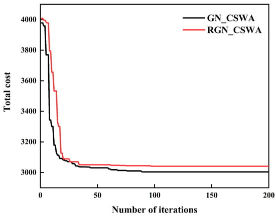
Figure 8.
Convergence curves of two algorithms.
5.5. Experimental Analysis Based on Different Parameter Settings
Based on the scale of the problem instances, the population sizes were set to 10, 20, 30, 40, and 50. The GN_CSWA, GA, ACO, and GA_GWO algorithms were independently run 10 times for each population size based on the C101 instance to ensure the statistical reliability of the experimental results, as shown in Table 10. The table lists the average total cost of each algorithm from the 10 independent runs. The experimental results indicate that GA performs best with a population size of 40; ACO yields better results with a population size of 50; and GA_GWO performs better with a population size of 40. Therefore, the population sizes for GA, ACO, and GA_GWO were set to 40, 50, and 40, respectively. Based on the experimental results, the population size had little impact on the performance of the GN_CSWA. However, considering the limited computational resources, the population size for GN_CSWA was set to 10 to balance algorithm performance and computational overhead. To more clearly illustrate the differences in total cost for the four algorithms at different population sizes, the average total cost of each algorithm at various population sizes is plotted in Figure 9, providing a more intuitive comparison of their performance across different population sizes.

Table 10.
Analysis of experimental results for four algorithms based on different population sizes.
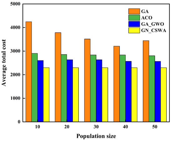
Figure 9.
Comparison graph of average total costs of four algorithms based on different population sizes.
To evaluate the impact of different parameter settings on the performance of the GN_CSWA, this study designed eight groups of comparative experiments with varying parameter combinations. Each key parameter was set at two levels (high and low) to systematically examine how changes in parameters affect algorithm performance. Each group of experiments was independently run 10 times based on the benchmark instance C101, and the results are presented in Table 11. The average total cost shown in the table represents the mean value obtained from 10 independent runs for each parameter group. The experimental results indicate that the algorithm exhibits relatively small performance fluctuations under different parameter combinations, suggesting that GN_CSWA has good stability. Since the parameter configuration in Group 8 achieved the best performance in terms of total cost, it was selected as the final parameter setting for GN_CSWA in this study. The optimal vehicle collecting routes obtained under this configuration are illustrated in Figure 10, where different colors represent the collecting routes of different vehicles.

Table 11.
Analysis of experimental results of GN_CSWA under different parameter settings.
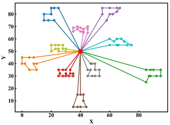
Figure 10.
Collection path graph with different colors representing different vehicles.
5.6. Comparative Experimental Analysis of Algorithms Based on Solomon Classic Datasets
To verify the effectiveness of the proposed GN_CSWA, this study employs five algorithms (GA, ACO, HSATA, GA_GWO, and GN_CSWA) as well as the commercial optimization solver Gurobi to solve benchmark instances R101, C101, and RC101. The experimental results of the six methods are compared and analyzed, as shown in Table 12. In the table, the average total cost refers to the average value obtained from ten independent runs of each heuristic algorithm on each instance. Since Gurobi, as a commercial solver, has deterministic characteristics and produces consistent results under the same problem settings, its result from a single run is used as a reference. The experimental results show that GN_CSWA achieves the lowest total cost in all three instances (R101, C101, and RC101), indicating better solution performance. In addition, based on the variance values of the results from each algorithm, GN_CSWA demonstrates higher stability.

Table 12.
Experimental results from different instances.
To verify the reliability of the experimental results obtained by the five algorithms, statistical significance tests were conducted on the total cost data of all algorithms across each instance. Before performing the significance tests, a normality test was first carried out. The results indicated that some of the data did not satisfy the assumption of normal distribution; therefore, the Kruskal–Wallis H test was employed. With a significance level set at , the p-values obtained from the nonparametric test were , , and , all of which are less than 0.05. This indicates that the GN_CSWA significantly outperforms the other four algorithms regarding experimental results, and the differences are statistically significant. To provide a more intuitive comparison of the performance differences among the six methods on different problem instances, the optimal total costs obtained from 10 independent runs of the five algorithms, along with the optimal result of the Gurobi commercial solver, are plotted in Figure 11. This figure demonstrates the solution performance of each method across various problem instances.
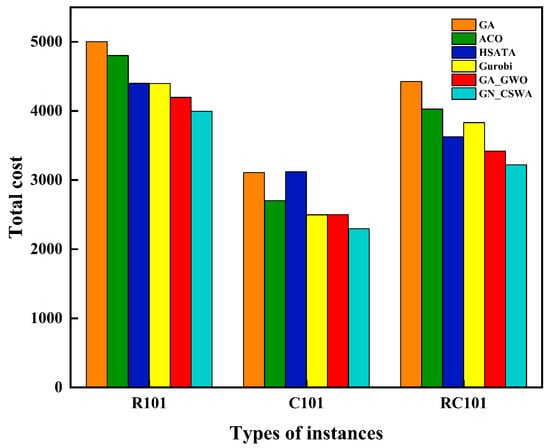
Figure 11.
Total cost comparison based on different instances.
5.7. Comparative Experimental Analysis of Algorithms Based on Real Map Dataset
To verify the effectiveness of GN_CSWA in real-world applications, this study applies five algorithms (GA, ACO, HSATA, GA_GWO, and GN_CSWA) and one commercial solver, Gurobi, to solve and analyze a real-map-based instance. The experimental results are presented in Table 13. In the table, the last row “TR” indicates the solution time required by each algorithm, measured in hours; the definitions of the other parameters are consistent with those in Table 8. The “Optimal” value represents the best solution obtained from 10 independent runs of each algorithm, while the “Average” value refers to the average of the 10 results. Since Gurobi is a deterministic solver, it produces consistent results under the same problem settings; thus, only a single run result is used for analysis. The experimental results show that compared with the four other algorithms and the commercial solver Gurobi, GN_CSWA achieves the best performance in terms of the number of vehicles used, total transportation cost, total travel distance, total fuel consumption, total carbon emission cost, and total time penalty cost. The only exception is the flower deterioration cost (CD), which is slightly higher than that of the other methods. This is because increasing the number of vehicles can reduce the number of customers served by each vehicle, thereby shortening customer waiting time and reducing flower deterioration. However, more vehicles also lead to increased transportation costs and carbon emissions. Therefore, GN_CSWA considers multiple factors during the solution process and identifies better solutions by balancing flower deterioration cost and overall operational cost. In addition to its strong performance in cost optimization, GN_CSWA also demonstrates good computational efficiency. Although all six methods require a relatively long runtime due to the complexity of the optimization objectives and limitations of the computing environment, GN_CSWA achieves significantly better efficiency compared to the other methods. It is capable of generating higher-quality routing solutions in a shorter time. These solutions not only require fewer vehicles and shorter travel distances but also effectively reduce fuel consumption and carbon emission costs.

Table 13.
Parameter analysis of experimental results for different algorithms.
Figure 12 shows the convergence curves of the optimal solutions obtained by running five algorithms independently 10 times on real map instances. As seen from the figure, GA performs poorly because its search operators only use PMX crossover and inversion mutation operations, leading to high randomness. Next is ACO, where the traditional ACO algorithm has a slow convergence speed and is prone to getting trapped in local optima. In contrast, HSATA and GA_GWO show improved performance over GA and ACO by utilizing large neighborhood search operators. However, although the operators of HSATA and GA_GWO consider spatial distance, they do not fully account for other factors, such as time distance, that impact the optimization results. GN_CSWA significantly improves both convergence speed and solution quality by integrating search operators that consider multiple factors, including spatial, temporal, and intra- and inter-subroute elements. Moreover, GN_CSWA generates initial solutions using both random and nearest neighbor algorithms, which results in an initial solution that is clearly better than those of the other four algorithms. With this better starting point, GN_CSWA can converge more quickly and obtain better solutions, thereby significantly reducing the total cost.
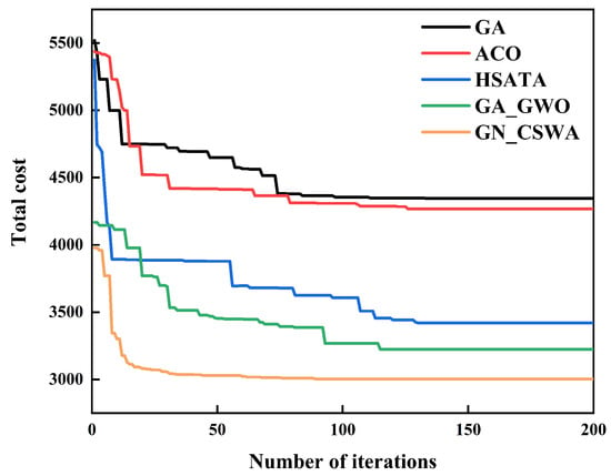
Figure 12.
Convergence curves of five algorithms based on real instances.
6. Conclusions and Future Works
Cold chain logistics generally faces the challenges of high energy consumption and emissions. With the establishment of China’s “dual carbon goals,” the national advocacy for green and sustainable development has been increasingly strengthened, and the transformation of logistics enterprises toward a low-carbon economy has become an inevitable trend. Against this background, this study addresses the existing limitations in cold chain logistics and proposes corresponding solutions from multiple perspectives, including the environment, enterprises, customers, and real-map scenarios. The specific research contents are as follows:
(1) A green cold chain routing planning model is constructed, which comprehensively considers multiple factors such as fixed cost, refrigeration cost, transportation cost, carbon emission cost, flower deterioration cost, and time penalty cost. A hard time window constraint is introduced to strictly comply with customers’ service time requirements, thereby maximizing customer satisfaction.
(2) Regarding algorithm improvement, this study proposes the GN_CSWA, which combines random generation with the nearest neighbor algorithm to generate diverse and high-quality initial solutions. Under the conditions of considering time and distance factors, the algorithm integrates GA, LNS, and SWO to enhance both global search capability and local optimization performance. The algorithm demonstrates superior solving performance in the routing optimization problem.
(3) For algorithm performance verification, the GN_CSWA is compared with GA, ACO, HSATA, GA_GWO, and the commercial solver Gurobi, based on Solomon benchmark instances and real map instances. The experimental results show that the GN_CSWA not only effectively reduces the total cost and carbon emissions of flower transportation but also performs well in terms of convergence speed and stability.
Although this paper has achieved certain results in cold chain logistics routing and algorithm optimization, there is still room for further improvement. Future research will focus on the following directions: First, the algorithm will undergo systematic testing on the original benchmark problem and be compared with known optimal solutions to further verify its effectiveness. Second, dynamic factors such as customer demand and time variations will be introduced into the model and the test instances will be expanded to include more than 1000 customers in order to enhance the model’s and algorithm’s adaptability and practical application value. Through these studies, this paper aims to provide more systematic and effective theoretical and methodological support for the development of low-carbon logistics and promote continuous innovation and intelligent transformation in the cold chain logistics field.
Author Contributions
M.L. writing—review and editing, data curation, writing—original draft preparation, visualization; S.W. conceptualization, methodology, supervision. All authors have read and agreed to the published version of the manuscript.
Funding
This research was funded by Yunnan Provincial Department of Science and Technology (Grant No. 202302AD080006, 202302AQ370003-4).
Data Availability Statement
The data come from the Solomon Benchmark Dataset and the OpenStreetMap website. The datasets used during the current study are available from the corresponding author upon reasonable request.
Conflicts of Interest
The authors declare no conflicts of interest.
References
- Su, Y.; Ye, Y.; Li, R.; Bai, J.; Ji, X.; Zhao, Y.; Wang, J.; He, G. Analysis of the Current Situation and Development Strategies of the Flower Industry in Kunming. Agric. Sci. Technol. Commun. 2023, 4, 18–22. [Google Scholar]
- Wu, J.; Liu, G.; Marson, A.; Fedele, A.; Scipioni, A.; Manzardo, A. Mitigating Environmental Burden of the Refrigerated Transportation Sector: Carbon Footprint Comparisons of Commonly Used Refrigeration Systems and Alternative Cold Storage Systems. J. Clean. Prod. 2022, 372, 133514. [Google Scholar] [CrossRef]
- Han, J.W.; Zuo, M.; Zhu, W.Y.; Zuo, J.H.; Lü, E.L.; Yang, X.T. A Comprehensive Review of Cold Chain Logistics for Fresh Agricultural Products: Current Status, Challenges, and Future Trends. Trends Food Sci. Technol. 2021, 109, 536–551. [Google Scholar] [CrossRef]
- Garside, A.K.; Ahmad, R.; Muhtazaruddin, M.N.B. A Recent Review of Solution Approaches for Green Vehicle Routing Problem and Its Variants. Oper. Res. Perspect. 2024, 12, 100303. [Google Scholar] [CrossRef]
- Gülmez, B.; Emmerich, M.; Fan, Y. Multi-Objective Optimization for Green Delivery Routing Problems with Flexible Time Windows. Appl. Artif. Intell. 2024, 38, 2325302. [Google Scholar] [CrossRef]
- Awad, M.; Ndiaye, M.; Osman, A. Vehicle Routing in Cold Food Supply Chain Logistics: A Literature Review. Int. J. Logist. Manag. 2021, 32, 592–617. [Google Scholar] [CrossRef]
- Dantzig, G.B.; Ramser, J.H. The Truck Dispatching Problem. Manag. Sci. 1959, 6, 80–91. [Google Scholar] [CrossRef]
- Beheshti, Z.; Shamsuddin, S.M.H. A Review of Population-Based Meta-Heuristic Algorithms. Int. J. Adv. Soft Comput. Appl. 2013, 5, 1–35. [Google Scholar]
- Salehi Sarbijan, M.; Behnamian, J. Emerging Research Fields in Vehicle Routing Problem: A Short Review. Arch. Comput. Methods Eng. 2022, 30, 2473–2491. [Google Scholar]
- Ngoo, C.M.; Goh, S.L.; Sabar, N.R.; Hijazi, M.H.A.; Kendall, G. A Survey of Mat-Heuristics for Combinatorial Optimisation Problems: Variants, Trends and Opportunities. Appl. Soft Comput. 2024, 164, 111947. [Google Scholar] [CrossRef]
- Solomon, M.M. VRPTW Benchmark Problems. Available online: https://www.sintef.no/projectweb/top/vrptw/solomon-benchmark/ (accessed on 20 April 2025).
- Hou, L.; Zhang, Z.; Xu, Y. Cold Chain Product Distribution Route Optimization Considering Time Windows Based on Genetic Algorithm. Logist. Technol. 2020, 39, 72–78. [Google Scholar]
- Qi, C.; Hu, L. Optimization of Vehicle Routing Problem for Emergency Cold Chain Logistics Based on Minimum Loss. Phys. Commun. 2020, 40, 101085. [Google Scholar] [CrossRef]
- Song, M.-X.; Li, J.-Q.; Han, Y.-Q.; Han, Y.-Y.; Liu, L.-L.; Sun, Q. Metaheuristics for Solving the Vehicle Routing Problem with Time Windows and Energy Consumption in Cold Chain Logistics. Appl. Soft Comput. 2020, 95, 106561. [Google Scholar]
- Du, C.; Li, Y. Research on Cold Chain Distribution Routing Problem Based on Customer Satisfaction and Minimum Loss. Ind. Eng. Manag. 2020, 25, 163–171. [Google Scholar]
- Ji, L.; Wang, Q.; Zhou, H.; Zheng, M. Cold Chain Fruit Routing Optimization Considering Customer Satisfaction. J. Zhejiang Univ. Sci. A 2021, 55, 307–317. [Google Scholar]
- Wu, N.; Dai, H.; Li, J.; Jiang, Q. Multi-Objective Optimization of Cold Chain Logistics Distribution Routing Considering Time Tolerance. J. Traffic Transp. Eng. 2023, 23, 275–284. [Google Scholar]
- Chen, J.; Gui, P.; Ding, T.; Na, S.; Zhou, Y. Optimization of Transportation Routing Problem for Fresh Food by Improved Ant Colony Algorithm Based on Tabu Search. Sustainability. 2019, 11, 6584. [Google Scholar] [CrossRef]
- Zhang, L.-Y.; Tseng, M.-L.; Wang, C.-H.; Xiao, C.; Fei, T. Low-Carbon Cold Chain Logistics Using Ribonucleic Acid-Ant Colony Optimization Algorithm. J. Clean. Prod. 2019, 233, 169–180. [Google Scholar]
- Ning, T.; Gou, T.; Liu, X. Simulation Study on Fresh Agricultural Products Cold Chain Logistics Strategy Considering Low-Carbon Constraints. J. Syst. Simul. 2022, 34, 797–805. [Google Scholar]
- Yao, Q.; Zhu, S.; Li, Y. Green Vehicle-Routing Problem of Fresh Agricultural Products Considering Carbon Emission. Int. J. Environ. Res. Public Health. 2022, 19, 8675. [Google Scholar] [CrossRef]
- Fang, C.; Gu, X.; Cheng, S.; Wu, D. Research on Long-Distance Cold Chain Logistics Route Optimization Considering Transport Vibration and Refrigerant Carbon Emission. Procedia Comput. Sci. 2022, 214, 1262–1269. [Google Scholar] [CrossRef]
- Shao, X.; Lu, S. Optimizing Dual Distribution Scheme in Pharmaceutical Cold Chain for Cost and Carbon Emissions Reduction. Appl. Sci. 2023, 13, 5524. [Google Scholar] [CrossRef]
- Xiao, Y.; Zhao, Q.; Kaku, I.; Xu, Y. Development of a Fuel Consumption Optimization Model for the Capacitated Vehicle Routing Problem. Comput. Oper. Res. 2012, 39, 1419–1431. [Google Scholar] [CrossRef]
- Abdel-Basset, M.; Mohamed, R.; Jameel, M.; Abouhawwash, M. Spider Wasp Optimizer: A Novel Meta-Heuristic Optimization Algorithm. Artif. Intell. Rev. 2023, 56, 11675–11738. [Google Scholar] [CrossRef]
- Mohamed, E.A.; Braik, M.S.; Al-Betar, M.A.; Awadallah, M.A. Boosted Spider Wasp Optimizer for High-Dimensional Feature Selection. J. Bionic Eng. 2024, 21, 2424–2459. [Google Scholar] [CrossRef]
- Sui, J.; Tian, Z.; Wang, Z. Multiple Strategies Improved Spider Wasp Optimization for Engineering Optimization Problem Solving. Sci. Rep. 2024, 14, 29048. [Google Scholar] [CrossRef]
- Ekinci, S.; Izci, D.; Turkeri, C.; Ahmad, M.A. Spider Wasp Optimizer-Optimized Cascaded Fractional-Order Controller for Load Frequency Control in a Photovoltaic-Integrated Two-Area System. Mathematics 2024, 12, 3076. [Google Scholar] [CrossRef]
- Qi, Y.; Cai, Y.; Cai, H.; Huang, H. Discrete Bat Algorithm for Vehicle Routing Problem with Time Windows. J. Electron. 2018, 46, 672–679. [Google Scholar]
- Li, Y.; Lim, M.K.; Tseng, M.L. A Green Vehicle Routing Model Based on Modified Particle Swarm Optimization for Cold Chain Logistics. Ind. Manag. Data Syst. 2019, 119, 473–494. [Google Scholar] [CrossRef]
- Alam, T.; Qamar, S.; Dixit, A.; Benaida, M. Genetic Algorithm: Reviews, Implementations, and Applications. arXiv 2020, 12673. [Google Scholar] [CrossRef]
- Sze, J.F.; Salhi, S.; Wassan, N. A Hybridisation of Adaptive Variable Neighbourhood Search and Large Neighbourhood Search: Application to the Vehicle Routing Problem. Expert Syst. Appl. 2016, 65, 383–397. [Google Scholar] [CrossRef]
- Gao, Y.; Li, Z.; Wang, H.; Hu, Y.; Jiang, H.; Jiang, X.; Chen, D. An Improved Spider-Wasp Optimizer for Obstacle Avoidance Path Planning in Mobile Robots. Mathematics 2024, 12, 2604. [Google Scholar] [CrossRef]
- Qi, M.; Lin, W.-H.; Li, N.; Miao, L. A Spatiotemporal Partitioning Approach for Large-Scale Vehicle Routing Problems with Time Windows. Transp. Res. Part E 2011, 48, 248–257. [Google Scholar] [CrossRef]
- Xia, X.; Qiu, H.; Xu, X.; Zhang, Y. Multi-Objective Workflow Scheduling Based on Genetic Algorithm in Cloud Environment. Inf. Sci. 2022, 606, 38–59. [Google Scholar] [CrossRef]
- Qi, R.; Li, J.; Wang, J.; Jin, H.; Han, Y. QMOEA: A Q-Learning-Based Multiobjective Evolutionary Algorithm for Solving Time-Dependent Green Vehicle Routing Problems with Time Windows. Inf. Sci. 2022, 608, 178–201. [Google Scholar] [CrossRef]
- Maroof, A.; Ayvaz, B.; Naeem, K. Logistics Optimization Using Hybrid Genetic Algorithm (HGA): A Solution to the Vehicle Routing Problem with Time Windows (VRPTW). IEEE Access. 2024, 12, 36974–36989. [Google Scholar] [CrossRef]
- Chen, J.; Liao, W.; Yu, C. Route Optimization for Cold Chain Logistics of Front Warehouses Based on Traffic Congestion and Carbon Emission. Comput. Ind. Eng. 2021, 161, 107663. [Google Scholar] [CrossRef]
- Liu, G.; Hu, J.; Yang, Y.; Xia, S.; Lim, M.K. Vehicle Routing Problem in Cold Chain Logistics: A Joint Distribution Model with Carbon Trading Mechanisms. Resour. Conserv. Recycl. 2020, 156, 104715. [Google Scholar] [CrossRef]
Disclaimer/Publisher’s Note: The statements, opinions and data contained in all publications are solely those of the individual author(s) and contributor(s) and not of MDPI and/or the editor(s). MDPI and/or the editor(s) disclaim responsibility for any injury to people or property resulting from any ideas, methods, instructions or products referred to in the content. |
© 2025 by the authors. Licensee MDPI, Basel, Switzerland. This article is an open access article distributed under the terms and conditions of the Creative Commons Attribution (CC BY) license (https://creativecommons.org/licenses/by/4.0/).