Article

Research on Stochastic Evolutionary Game and Simulation of Carbon Emission Reduction Among Participants in Prefabricated Building Supply Chains

1
School of Management, Shenyang Jianzhu University, Shenyang 110168, China
2
School of Civil Engineering, Shenyang Jianzhu University, Shenyang 110168, China
3
School of Business Administration, Liaoning Technical University, Huludao 125105, China
*
Author to whom correspondence should be addressed.
Appl. Sci. 2025, 15(9), 4982; https://doi.org/10.3390/app15094982
Submission received: 13 March 2025 / Revised: 26 April 2025 / Accepted: 28 April 2025 / Published: 30 April 2025

Abstract

:
Developing prefabricated buildings (PBs) and optimizing the construction supply chain represent effective strategies for reducing carbon emissions in the construction industry. Prefabricated building supply chain (PBSC) carbon reduction suffers from synergistic difficulties, limited rationality, and environmental complexity. Therefore, investigating carbon emission reduction in PBSC is essential. In this study, PBSC participants are divided into four categories according to the operation process. Gaussian white noise is introduced to simulate the random perturbation factors, and a four-way stochastic evolutionary game model is constructed and numerically simulated. The study found the following: Stochastic perturbation factors play a prominent role in the evolution speed of the agent; the emission reduction benefit and cost of the participant significantly affect the strategy selection; the operation status of the PBSC is the key to strategy selection, and it is important to pay attention to the synergy of the participants at the first and the last end of the PBSC; the influence of the external environment on strategies is mainly manifested in the loss caused and the assistance provided; and the information on emission reduction is an important factor influencing strategies. Finally, we provide suggestions for promoting carbon emission reduction by participants in the PBSC from the perspective of resisting stochastic perturbation, enhancing participants’ ability, and strengthening PBSC management; external punishment and establishing a cross-industry information sharing platform is more important than the reward.

1. Introduction

The current global climate situation is dire and demands urgent attention and governance [1]. China has placed great emphasis on carbon emission reduction, signing the Paris Agreement in 2016 and pledging a “dual-carbon” goal at the 75th United Nations General Assembly [2]. As a key pillar and high-energy-consuming sector of the national economy, the construction industry is a primary target for carbon emission reduction [3]. It actively promotes the development of prefabricated buildings and supply chain construction to meet industry requirements for reducing carbon emissions. However, PBSC carbon reduction still faces numerous challenges.
Firstly, PBSC coordination difficulties. PBSC faces problems due to the large number of participants and the complex coordination process of each link [4]. For example, suppliers and contractors struggle with variable transportation distances and component sizes [5]. Insufficient on-site inventory and unchangeable assembly processes cause stagnation in the construction process [6]. These difficulties result in uncertainty in PBSC participants’ various links, leading to progress, material and energy waste, and an inevitable increase in carbon emissions. The participants involved in the prefabricated building supply chain (PBSC) operation are the basic units to achieve carbon emission reduction [7]. Coordination within PBSC plays a vital role in its carbon reduction [8].
In addition, PBSC participants at all stages have limited rationality and different interests. In actual decision-making, PBSC participants have problems with insufficient information sharing and insufficient data utilization [9]. This leads them to make decisions based on limited resources, which increases the complexity of making decisions. PBSCs have different demands for benefit distribution [10], and all want to benefit more from carbon emission reduction. For example, prefabricated component suppliers aim to increase profits from raw materials, while constructors seek to reduce construction costs to boost revenue. This results in inconsistent emission reduction goals and benefit disputes among PBSC participants, hindering cooperation.
Finally, with regard to the complexity of the environment outside PBSC, policies, technologies, and markets all impact PBSC carbon reduction [8,11]. For example, carbon prices and subsidy imperfections create uncertainty about carbon reduction effects [11]. The uncertainty of market fluctuations and technological changes [12] make it difficult for participants to predict the future benefits of emission reduction, affecting emission reduction decisions.
To address the above issues, this paper develops a stochastic evolutionary game model to explore how PBSC participants interact under numerous challenges to achieve carbon reduction goals. The model parameters include supply chain coordination, participants’ interests, and interventions from external entities. This study aims to provide a decision-making basis for PBSC practitioners and suggest how external entities, such as governments, financial institutions, and research institutes, can support PBSC carbon emission reduction. This study enriches the scope of PBSC research and is significant for the long-term development of carbon emission reduction in the construction industry.
The structure of the rest of this study is as follows: Section 2 summarizes the literature on PBSC, carbon reduction in PBSC, and evolutionary games. Section 3 illustrates the game relationship between the agents in PBSC. An evolutionary game model is established, then Gaussian white noise is introduced to construct a stochastic evolutionary game model, and finally, the model is analyzed. In Section 4, numerical simulation experiments are performed to model the strategy evolution of the agents under different conditions. Section 5 summarizes and analyzes the simulation results and makes recommendations. Finally, Section 6 concludes this study.

2. Literature Review

2.1. PBSC

The PBSC encompasses all participants and links throughout the process of PB projects, from project approval, feasibility demonstration, and design; to procurement, processing, and manufacturing of raw materials; to production, transportation, and storage of prefabricated components; to on-site assembly and construction management; and finally to delivery, use, end-of-life dismantling, and recycling [13]. It is a functional network structure that connects project owners, general contractors, construction units, and others through capital flow, logistics, and information flow [14,15,16,17]. Based on scholars’ definitions of the PBSC, its basic framework is established, and participants are categorized into four types of agents according to the supply chain operation process [18,19], as shown in Figure 1.

2.2. Carbon Reduction in PBSC

Prefabricated buildings reduce carbon emissions at all stages, driven by the roles of PBSC participants. Prefabricated buildings aid in decarbonizing the construction industry and enhancing productivity and sustainability [20]. In 2024, China took the development of PBs as one of the measures to save energy and reduce carbon emissions in buildings [21]. PBs can save building materials [22], reducing greenhouse gas emissions during materialization. PBs can effectively reduce the operational energy consumption of buildings [23]. Prefabrication has advantages in reducing construction waste and waste recycling [24]. The composition of carbon emissions in the life cycle of PBs is complex [25,26], involving multiple segments and participants with complex mechanisms of collaboration and action [27].
Scholars have conducted a lot of research on the factors influencing carbon emission reduction within the supply chain, which provides the research basis for this paper. External regulations significantly affect low-carbon technology co-innovation [28]. Information disclosure and sharing substantially impact carbon emissions within the supply chain [29,30,31]. Financial institutions improve the enthusiasm of supply chain members to reduce emissions by influencing their abatement costs [32,33]. Government subsidies promote technological innovation, thus effectively promoting emission reduction by supply chain members [34,35]. Supply chain information synergy can effectively reduce carbon emissions [36]. Internal coordination and external supply chain intervention jointly affect emission reduction capacity and targets [28].
However, current research primarily focuses on the emission reduction decision-making of enterprises such as precast manufacturers and contractors. They focus more on the role of external governments on individual PBSC participants. Few studies examine the interactions among PBSC participants’ emission-reduction decisions, with a lack of research on participants’ decisions across the entire PBSC. Regarding influencing factors, current studies focus more on governmental and market factors, while fewer scholars consider the impact of emission reduction information and PBSC synergy on carbon emission reduction. Wang et al. used an evolutionary game to study the low-carbon decision-making of precast manufacturers, and pointed out that cost—less than—and government incentives are the main influences on the adoption of low-carbon technologies [37]. Liu et al. used SEM to study the drivers of carbon emission reduction in PBSC, finding that technological factors significantly impact emission reduction, followed by economic and social factors [38]. Wang, D. and Wang, X. examined the effects of government subsidies on the low-carbon decisions of project contractors and precast manufacturers, and found that unit cost subsidies help reduce carbon emissions, while volume rate subsidies help reduce carbon emission intensity [39]. Du et al. analyzed the impact of environmental policies on PBSC carbon emission reduction using the SD model, and found that subsidies play a leading role in carbon emission reduction, while investment in technology and carbon pricing can also increase benefits [11]. Sun et al. developed a Stackelberg model to analyze PB manufacturers and retailers’ carbon emission reduction decisions, focusing on the effects of carbon quotas and government subsidies [40].

2.3. Evolutionary Game Theory

Currently, game theory is widely used to study the interaction mechanisms of strategies among supply chain participants and has applications in carbon emission reduction. Lin and Liu explored the strategic choices and evolutionary stabilization paths of carbon emission reduction inputs of supply chain agents by establishing an evolutionary game model [41]. Zhang and Liang constructed a supply chain game model of suppliers, manufacturers, and retailers to study the factors affecting low-carbon production [42]. Wang and Li established an evolutionary game model between manufacturers and suppliers to explore how to promote corporate green innovation to improve their willingness to cooperate in carbon emission reduction [43]. Wang and Wang considered the issues of bounded rationality and fairness and established an evolutionary game model for manufacturers and retailers to analyze their low-carbon effort decisions [44]. The evolutionary game is an effective method for studying how to implement emission reduction decisions among supply chain participants.
PBSC is challenging to coordinate [4,5,6], and each participant has uncertainty [9,10]. Policies, markets, and technological changes [8,11,12] will all interfere with decision-making as external uncertainties. These stochastic factors are long-standing and unavoidable, requiring participants to make decisions based on their judgment amidst these disturbances. In the ideal deterministic evolutionary game model, it is difficult to consider these random factors. Therefore, we introduce random perturbation factors into the game system to construct a more realistic stochastic evolutionary game. This approach has been applied by many scholars [45,46,47,48,49,50]. Wang and Tai constructed a stochastic evolutionary game model to address uncertainty in the live broadcasting environment [47]. Gao et al. introduced stochastic factors for model optimization to overcome sudden natural events and policy mutations [48]. This method has been applied in studies of carbon reduction [49,50], supply chains [46], and the construction industry [45]. In conclusion, the stochastic evolution game is applicable to analyzing the participants’ carbon emission reduction in PBSC.

2.4. Research Gap

Scholars have conducted some research on PBSC carbon emission reduction, providing a sufficient research basis, but there are still the following shortcomings:
  • Current research demonstrates that participants in each link of the PBSC, from design to dismantling, can reduce carbon emissions. Still, there is less research on how the emission reduction strategies of these participants interact with each other. Compared with studies on secondary and tertiary supply chains, the model constructed in this paper covers the entire PBSC, rather than only partial links or conceptualized upstream and downstream enterprises. This paper’s four-way evolutionary game model reflects participants’ emission reduction strategy choices in the whole PBSC, which is more comprehensive.
  • Besides the impact of PBSC participants and external institutions on carbon emission reduction, emission reduction information and PBSC synergy also have a significant effect. Most current studies consider the impact of policy and social factors, such as subsidies, taxes, carbon trading, etc., on carbon emission reduction in PBSC, ignoring the effect of emission reduction information. In addition, current research exists on how synergies and free-rider effects in the supply chain play a role in carbon emission reduction, but there are fewer studies for PBSCs.
  • Most studies recognize the impact of stochastic disturbances on carbon emission reduction in PBSCs. Still, few scholars have included them in a systematic analysis to explore the interaction of players’ emission reduction strategies. Most of the existing studies construct evolutionary game models in an ideal state, which lacks authenticity. In addition, there are still fewer methods to study PBSC carbon emission reduction using stochastic evolutionary game models.
This study introduces a four-level stochastic evolutionary game model of PBSC, which is innovative in its completeness, comprehensiveness, and realism. Unlike two-level and three-level models, this four-level model encompasses a broader range of PBSC segments and scopes. It considers the impact of both internal and external factors on carbon emission reduction, offering a more comprehensive analysis. The incorporation of Gaussian white noise to simulate disturbances endows the model with practicality by reflecting real-world uncertainties in enterprise decision-making, thus transcending the idealized assumptions in traditional game models.

3. Model and Analysis

3.1. Problem Raising and Basic Assumptions

PBSCs contain many participants, which are categorized into four types based on their roles in the supply chain operation process: the Planning and Designing Party (X), Production and Construction Party (Y), Operation and Maintenance Party (Z), and Dismantling and Recycling Party (U) [14,15,16,17]. The Planning and Designing Party (X) comprises enterprises that organize, plan, finance, and design the PB construction process, including owners, design institutes, and consultants. The Production and Construction Party (Y) includes PB component manufacturers, transporters, and contractors involved in the physicalization phase of PBs, responsible for production, transportation, and assembly. The Operation and Maintenance Party (Z) comprises enterprises responsible for PB operation and maintenance after delivery, such as property and maintenance companies. The Dismantling and Recycling Party (U) is accountable for breaking down the PB at the end of its life and recycling construction waste, including dismantlers and recyclers. Their relationships are complex, and they face the dilemma of interest disputes in PBSC carbon reduction. Each agent’s costs, benefits, and ability to implement emission reductions [50,51], as well as external incentives, support, and environmental regulation, all impact the agent [51,52,53]. In addition, there is an interaction of interests in the implementation of emission reduction strategies: The contractual relationship between X and the other three includes penalties for non-compliance, which influences the approach of the participant from within the PBSC; the simultaneous implementation of carbon emission reduction by multiple parties enhances synergies and generates joint benefits [54]; the upstream party’s implementation of carbon emission reduction has a spillover effect, from which the downstream party benefits through the “free-riding” effect [23,55]. Based on the above analysis, the following basic assumptions are established, and parameters are set:
Hypothesis 1. 
Agents of the evolutionary game are the Planning and Designing Party (X), the Production and Construction Party (Y), the Operation and Maintenance Party (Z), and the Dismantling and Recycling Party (U), all of which are bounded rationally. They will choose their own strategies, evolving into the optimal strategy over time.
Hypothesis 2. 
Each agent has either an abatement strategy or no abatement strategy. The probability that X, Y, Z, and U implement the “abatement” strategy is   x , y , z , u , respectively, and  x , y , z , u [ 0 , 1 ] . The probability that they implement the “no-abatement” strategy is  1 x , 1 y , 1 z , 1 u , respectively.
The parameters, definitions, and detailed explanations are presented in Table 1.

3.2. Construction of a Four-Way Evolutionary Game Model

3.2.1. Construction of the Payoff Matrix

Based on the basic assumptions and parameters in the previous section, the following assumptions are made to establish a four-way evolutionary game model:
H1. 
When the agent implements the “abatement” strategy, the support it receives from the external environment is  Π i = J i + Δ C i + D γ i λ i . When the agent reduces emissions, the government provides green subsidies, and industry bodies offer reputational incentives, which can enhance economic or reputational strength. When the agent reduces emissions, it inevitably generates financing, purchases of equipment, and trades in environmentally friendly materials. Financial institutions streamline processes to cut costs, research bodies reduce equipment costs via joint R&D, and suppliers offer long-term deals for mutual benefits. These measures reduce the abatement cost to the agent. When an agent reduces emissions, it must acquire information on technologies, prices, and policies. The agent’s information acquisition is bounded by availability and gathering ability. Post-acquisition, the agent analyzes it to make decisions, with the benefit being  D γ i λ i [56]. When the agent implements the “abatement” strategy, the cost it pays is  C i , and the benefit it obtains is  E i , where  i { X , Y , Z , U } . These are the direct costs and benefits associated with implementing emission reduction. Costs include using eco-friendly materials, acquiring raw resources, and introducing advanced technology. Benefits are direct gains from emission reductions, such as energy savings, efficiency improvements, and enhanced market popularity.
H2. 
If any two agents in PBSC implement the “abatement” strategy, the value-added benefit to agent  i  who implements the “abatement” strategy is  β i j E i , where  i { X , Y , Z , U } , j { X , Y , Z , U } , i j   [41]. The value-added benefits accumulate if multiple agents implement the “abatement” strategy. When two agents reduce emissions simultaneously, they form an alliance, share information, and collaborate on construction plans. This optimizes PBSC operation efficiency, reduces communication costs, and yields joint emission reduction benefits.
H3. 
When upstream party  j  implements an “abatement” strategy and downstream party  i  implements a “no-abatement” strategy, downstream party  i  receives a free-rider benefit of  α i j E i , where  i { Y , Z , U } , j { X , Y , Z } , i j   [41]. For example, green design on the design side reduces PB energy consumption and operating costs, while green construction by the construction side eases demolition difficulties and indirectly boosts revenue. For downstream parties, free-rider benefits from different upstream parties can accumulate.
H4. 
When a party implements a “no-abatement” strategy, it incurs a loss of  G i ( i { X , Y , Z , U } ) , e.g., a fine from the regulator due to actions taken by organizations external to the PBSC [28]. Specifically, contractors not implementing abatement strategies will pollute the environment during construction, endangering neighboring residents’ health and leading to complaints. Excessive contractor contamination can lead to fines or corrective action deadlines from regulators, causing financial losses. High energy consumption during operation and maintenance can reduce consumer willingness to buy, affecting revenue.
H5. 
When X implements an “abatement” strategy, the downstream party will be contractually obligated to pay a penalty of  N i ( i { Y , Z , U } )  when it implements a “no-abatement” strategy. If the builder decides to reduce emissions, the contract will include relevant agreements, such as using environmentally friendly materials and specifying work quality requirements. The contractor must pay liquidated damages under the contract if it fails to perform.
Figure 2 depicts the framework for constructing a model payoff matrix based on parameters and assumptions. Each agent of the game has two strategies: “abatement” and “no-abatement”. The four agents form 16 strategy sets. The payoff of each agent in each strategy set is  L n i ( n [ 1 , 16 ] ; i { X , Y , Z , U } ) . Each strategy set, denoted by (x, y, z, u), comprises four strategies, where 0 signifies “no-abatement” and 1 signifies “abatement”. The mapping of strategy sets to payoffs is presented in Table 2. The payoff matrix is shown in Table 3 and Table 4. Consider the strategy set (1, 1, 1, 1) in Table 3, where all four players implement abatement measures. The corresponding payoffs for the four parties are  L 1 X , L 1 Y , L 1 Z , and  L 1 U , respectively. All agents incur the cost  C i  and receive the benefit  E i . All agents receive incentives  J i , assistance  Δ C i , and process emission reduction information to gain benefits  D γ i λ i . The total external benefits are  Π i = J i + Δ C i + D γ i λ i . Since all four agents choose to reduce emissions, each agent can obtain value-added benefits from the other three agents. For instance, the value-added benefits of collaborative emission reduction obtained by X are  ( β X Y + β X Z + β X U ) E X . The payoff of X is  L 1 X = E X C X + Π X + ( β X Y + β X Z + β X U ) E X . The detailed composition of the payoffs is presented in Table 3.

3.2.2. Replicator Dynamics Equation

Based on the payoff matrix in Table 3 and Table 4, the expected payoffs of X for choosing the “abatement” and “no-abatement” strategies are  E x 1  and  E x 2 , respectively, and the average payoff of the strategy choices is  E x . The replicator dynamic equation for X is  F ( x ) .
E x 1 = y z u L 1 x + y z ( 1 u ) L 2 x + y ( 1 z ) u L 3 x + y ( 1 z ) ( 1 u ) L 4 x + ( 1 y ) z u L 5 x + ( 1 y ) z ( 1 u ) L 6 x + ( 1 y ) ( 1 z ) u L 7 x + ( 1 y ) ( 1 z ) ( 1 u ) L 8 x
E x 2 = y z u L 9 x + y z ( 1 u ) L 10 x + y ( 1 z ) u L 11 x + y ( 1 z ) ( 1 u ) L 12 x + ( 1 y ) z u L 13 x + ( 1 y ) z ( 1 u ) L 14 x + ( 1 y ) ( 1 z ) u L 15 x + ( 1 y ) ( 1 z ) ( 1 u ) L 16 x
E x = x E x 1 + ( 1 x ) E x 2
F ( x ) = d x d t = x E x 1 E x = x ( 1 x ) [ ( 1 + y β X Y + z β X Z + u β X U ) E X C X + Π X + ( 1 y ) N Y + ( 1 z ) N Z + ( 1 u ) N U + G X ]
Similarly, the replicator dynamic equations for Y, Z, and U strategy choices are  F ( y ) F ( z ) , and  F ( u ) , respectively.
F ( y ) = d y d t = y E y 1 E y = y ( 1 y ) [ ( 1 + x β Y X + z β Y Z + u β Y U ) E Y C Y + Π Y + G Y + x N Y x α Y X E Y ]
F ( z ) = d z d t = z E z 1 E z = z ( 1 z ) [ ( 1 + x β Z X + y β Z Y + u β Z U ) E Z C Z + Π Z + G Z + x N Z ( x α Z X + y α Z Y ) E Z ]
F ( u ) = d u d t = u E u 1 E u = u ( 1 u ) [ ( 1 + x β U X + y β U Y + z β U Z ) E U C U + Π U + G U + x N U ( x α U X + y α U Y + z α U Z ) E U ]

3.3. Construction and Analysis of Stochastic Evolutionary Game Model

3.3.1. Game Model Establishment

The extended supply chain and long PB operation time introduce multiple interferences in decision-making: the government’s allocation of carbon subsidies and quotas [59], carbon taxes settings [60,61] subsidies and tax incentives [61,62], low-interest loans from financial institutions to PC manufacturers [62], labor quantity and quality [62,63], advanced construction technology applications [62], and market fluctuations [12]. In addition, participants in PBSC have subjective uncertainties, such as developers’ environmental awareness [60], additional costs of seeking partners [63], and suppliers’ strategic preference [64], which are random disturbance factors. For PBSC, these random disturbance factors are long-term and unavoidable and cannot be ignored in practice. Gaussian white noise is a zero-mean, constant-variance random noise with independent, identical distribution at each time and a flat spectrum [65]. Gaussian white noise’s simplicity and various features make it suitable for modeling random perturbation factors [66]. The randomness and uncertainty of white Gaussian noise correspond to the unpredictability of disturbance factors; its stable statistical properties reflect the long-term existence of random factors; and spectral flatness allows adjustment of noise intensity to simulate the game system under different random disturbances. Therefore, Gaussian white noise is applied to simulate random perturbation factors to construct a stochastic evolutionary game model [45,46,47,48]. Referring to Sun et al. [67], since  x , y , z , u [ 0 , 1 ] , terms like 1 − x in replicator dynamic equations do not affect the evolutionary process, and are omitted. The replicator dynamic equations for X, Y, Z, and U, after being affected by random perturbations, are shown in Equations (8)–(11):
d x t = x ( t ) [ ( 1 + y β X Y + z β X Z + u β X U ) E X C X + Π X + ( 1 y ) N Y + ( 1 z ) N Z + ( 1 u ) N U + G X ] d t + σ x t d w t
d y t = y ( t ) [ ( 1 + x β Y X + z β Y Z + u β Y U x α Y X ) E Y C Y + Π Y + G Y + x N Y ] d t + σ y t d w t
d z t = z ( t ) [ ( 1 + x β Z X + y β Z Y + u β Z U x α Z X y α Z Y ) E Z C Z + Π Z + G Z + x N Z ] d t + σ z t d w t
d u t = u ( t ) [ ( 1 + x β U X + y β U Y + z β U Z x α U X y α U Y z α U Z ) E U C U + Π U + G U + x N U ] d t + σ u t d w t
σ  in the above equation denotes the random perturbation intensity.  w t  follows a one-dimensional Brownian motion and reflects the effect of the random disturbance factor.  d w t  denotes Gaussian white noise, and the increment  Δ w t = w t + h w t  follows a normal distribution when  t > 0  and the step size  h > 0 .

3.3.2. Game Model Analysis

Model stability analysis is based on the existence and uniqueness of solutions. The existence and uniqueness of solutions to Equations (8)–(11) are proved using the local Lipschitz condition and the linear growth condition [68], and the proof procedure is shown in Appendix A. Thus, stability analysis can be performed.
For Equations (8)–(11), when  t = 0 , it results in  x ( t ) = y ( t ) = z ( t ) = u ( t ) = 0 . This shows that the zero solution is the equilibrium solution of the equation when there is no perturbation in the gaming system [67].
In practice, Gaussian white noise is bound to disturb the gaming system, which is therefore judged based on the stability theorem for stochastic differential equations [69,70,71].
Firstly, given the stochastic differential equation as shown in Equation (12)
d x t = f ( t , x ( t ) ) d t + g ( t , x ( t ) ) d w t , x t 0 = x 0
Let there exist a function  V ( t , x )  and positive constants  v 1 , v 2  such that  v 1 x p V ( t , x ) v 2 x p , t 0 .
Theorem 1. 
If there exists a positive constant  μ , such that  L V ( t , x ) μ V ( t , x ) , t 0 , then the zero solution of Equation (12) is a P-order moment exponentially stable, and  E x ( t , x 0 ) p < ( v 1 v 2 ) x 0 p e μ t , t 0  holds.
Theorem 2. 
If there exists a positive constant  μ , such that  L V ( t , x ) μ V ( t , x ) , t 0 , then the zero solution of Equation (12) is a P-order moment exponentially unstable, and  E x ( t , x 0 ) p ( v 1 v 2 ) x 0 p e μ t , t 0  holds.
According to the above theorem, taking  V t ( t , x ) = x , V t ( t , y ) = y , V t ( t , z ) = z , V t ( t , u ) = u ;   x , y , z , u [ 0 , 1 ] , v 1 = v 2 = 1 , p = 1  for Equations (8)–(11) yields Equations (13)–(16):
L V ( t , x ) = [ ( 1 + y β X Y + z β X Z + u β X U ) E X C X + Π X + ( 1 y ) N Y + ( 1 z ) N Z + ( 1 u ) N U + G X ] x
L V ( t , y ) = [ ( 1 + x β Y X + z β Y Z + u β Y U x α Y X ) E Y C Y + Π Y + G Y + x N Y ] y
L V ( t , z ) = [ ( 1 + x β Z X + y β Z Y + u β Z U x α Z X y α Z Y ) E Z C Z + Π Z + G Z + x N Z ] z
L V ( t , u ) = [ ( 1 + x β U X + y β U Y + z β U Z x α U X y α U Y z α U Z ) E U C U + Π U + G U + x N U ] u
If the P-order moment exponents of the zero solutions of Equations (13)–(16) are stable, then Equations (8) and (9) are satisfied. A more detailed demonstration process can be found in Appendix A.
x [ ( 1 + y β X Y + z β X Z + u β X U ) E X C X + Π X + ( 1 y ) N Y + ( 1 z ) N Z + ( 1 u ) N U + G X ] x
y [ ( 1 + x β Y X + z β Y Z + u β Y U x α Y X ) E Y C Y + Π Y + G Y + x N Y ] y
z [ ( 1 + x β Z X + y β Z Y + u β Z U x α Z X y α Z Y ) E Z C Z + Π Z + G Z + x N Z ] z
u [ ( 1 + x β U X + y β U Y + z β U Z x α U X y α U Y z α U Z ) E U C U + Π U + G U + x N U ] u
The condition satisfying Equation (17) is derived as X1 or X2 by performing the reduction computation. The derivation is shown in Appendix A.
X1. 
When  x ( 0 , 1 ]    and  β X Y E X N Y > 0  ,  y 1 ( 1 + z β X Z + u β X U ) E X + C X Π X N Y ( 1 z ) N Z ( 1 u ) N U G X / ( β X Y E X N Y ) and  0 1 ( 1 + z β X Z + u β X U ) E X + C X Π X N Y ( 1 z ) N Z ( 1 u ) N U G X   should be satisfied.
X2. 
When  x ( 0 , 1 ]  and  β X Y E X N Y < 0 y [ 1 ( 1 + z β X Z + u β X U ) E X + C X Π X N Y ( 1 z ) N Z ( 1 u ) N U G X ] / ( β X Y E X N Y ) and  1 ( 1 + z β X Z + u β X U ) E X + C X Π X N Y ( 1 z ) N Z ( 1 u ) N U G X 0  should be satisfied.
Similarly, the conditions for satisfying Equations (18)–(20) are Y1, Z1, and U1, respectively:
Y1. 
It should satisfy  z [ 1 ( 1 + x β Y X + u β Y U x α Y X ) E Y + C Y Π Y G Y x N Y ] / β Y Z E Y   and  0 1 ( 1 + x β Y X + u β Y U x α Y X ) E Y + C Y Π Y G Y x N Y .
Z1. 
It should satisfy   u [ 1 ( 1 + x β Z X + y β Z Y x α Z X y α Z Y ) E Z + C Z Π Z G Z x N Z ] / β Z U E Z   and  0 1 ( 1 + x β Z X + y β Z Y x α Z X y α Z Y ) E Z + C Z Π Z G Z x N Z .
U1. 
It should satisfy     x [ 1 ( 1 + y β U Y + z β U Z y α U Y z α U Z ) E U + C U Π U G U ] / ( β U X E U α U X E U + N U )   and  0 1 ( 1 + y β U Y + z β U Z y α U Y z α U Z ) E U + C U Π U G U .
If the P-order moment exponents of the zero solutions of Equations (13)–(16) are unstable, then
x [ ( 1 + y β X Y + z β X Z + u β X U ) E X C X + Π X + ( 1 y ) N Y + ( 1 z ) N Z + ( 1 u ) N U + G X ] x
y [ ( 1 + x β Y X + z β Y Z + u β Y U x α Y X ) E Y C Y + Π Y + G Y + x N Y ] y
z [ ( 1 + x β Z X + y β Z Y + u β Z U x α Z X y α Z Y ) E Z C Z + Π Z + G Z + x N Z ] z
u [ ( 1 + x β U X + y β U Y + z β U Z x α U X y α U Y z α U Z ) E U C U + Π U + G U + x N U ] u
The condition satisfying Equation (21) is derived as X3 or X4 by performing the reduction computation.
X3. 
When  x ( 0 , 1 ]  and  β X Y E X N Y > 0 y [ 1 ( 1 + z β X Z + u β X U ) E X + C X Π X N Y ( 1 z ) N Z ( 1 u ) N U G X ] / ( β X Y E X N Y )  and  1 ( 1 + z β X Z + u β X U ) E X + C X Π X N Y ( 1 z ) N Z ( 1 u ) N U G X β X Y E X N Y  should be satisfied.
X4. 
When  x ( 0 , 1 ]  and  β X Y E X N Y < 0 y [ 1 ( 1 + z β X Z + u β X U ) E X + C X Π X N Y ( 1 z ) N Z ( 1 u ) N U G X ] / ( β X Y E X N Y )  and  1 ( 1 + z β X Z + u β X U ) E X + C X Π X N Y ( 1 z ) N Z ( 1 u ) N U G X β X Y E X N Y  should be satisfied.
Similarly, the conditions for satisfying Equations (22)–(24) are Y2, Z2, and U2, respectively.
Y2. 
It should satisfy  z [ 1 ( 1 + x β Y X + u β Y U x α Y X ) E Y + C Y Π Y G Y x N Y ] / β Y Z E Y  and  1 ( 1 + x β Y X + u β Y U x α Y X ) E Y + C Y Π Y G Y x N Y β Y Z E Y .
Z2. 
It should satisfy  u [ 1 ( 1 + x β Z X + y β Z Y x α Z X y α Z Y ) E Z + C Z Π Z G Z x N Z ] / β Z U E Z  and  1 ( 1 + x β Z X + y β Z Y x α Z X y α Z Y ) E Z + C Z Π Z G Z x N Z β Z U E Z .
U2. 
It should satisfy  x [ 1 ( 1 + y β U Y + z β U Z y α U Y z α U Z ) E U + C U Π U G U ] / ( β U X E U α U X E U + N U )  and  1 ( 1 + y β U Y + z β U Z y α U Y z α U Z ) E U + C U Π U G U β U X E U α U X E U + N U .
When Condition 1 is satisfied, namely  { ( X 1 X 2 ) Y 1 Z 1 U 1 } , each agent chooses to implement the “no-abatement” strategy, and the game system reaches the state of (0, 0, 0, 0). At present, the proportion of emission-reducing enterprises in PBSC is low, and their willingness to reduce emissions is weak. For each entity, the benefits from implementing “abatement” are lower than those from “no-abatement”. This is the most pessimistic state when all the agents in PBSC are in a wait-and-see mode.
When Condition 2 is satisfied, namely  { ( X 3 X 4 ) Y 2 Z 2 U 2 } , each agent chooses to implement the “abatement” strategy, and the game system reaches the state of (1, 1, 1, 1). At present, the proportion of emission-reducing enterprises in PBSC is relatively high. For each agent, the benefits from implementing “abatement” exceed those from “no-abatement”. This is the ideal state in which all the agents in PBSC choose to implement an “abatement” strategy.
The data for Conditions 1 and 2 are presented in Table 5. Based on these datasets, 30 repeated simulations were conducted for each condition, with the results depicted in Figure 3. The stable states achieved in each simulation aligned with the analytical outcomes. On average, Conditions 1 and 2 required approximately 163 and 40 iterations, respectively, to reach stability. Due to random disturbance factors, fluctuations occurred after system stabilization, which were more pronounced in Condition 1, with a strategy probability fluctuation range of [0, 0.07]. In contrast, Condition 2 exhibited no fluctuations. This discrepancy arises because the parameters in Condition 2 were set in an overly ideal manner, rendering random disturbances insufficient to impact the strategy. Experiments validate the reliability of the stability analysis.
With other parameters held constant and only the intensity of random interference varied, the system evolution is depicted in Figure 4. The system’s final stability remains unaffected. However, as the interference intensity increases, the fluctuation range of strategy probabilities in the stable state also widens.
Random disturbance variables do not affect whether the system reaches a stabilization point. Unlike the traditional deterministic evolutionary game model [41], this model’s evolution to a stable point depends on agents’ influencing factors and strategic choices. This aligns with the actual scenario where businesses collaborate on PBSC carbon emission reduction based on observing each other’s choices.

3.4. Stochastic Taylor Expansion

Since nonlinear Itô stochastic differential equations cannot be directly solved analytically, the stochastic Taylor expansion is applied using the Eulerian method for numerical simulation. Therefore, the Taylor expansions for the Planning and Designing Party (X), the Production and Construction Party (Y), the Operation and Maintenance Party (Z), and the Dismantling and Recycling Party (U) can be derived as Equations (25)–(28), respectively:
x ( t n + 1 ) = x ( t n ) + h [ ( 1 + y β X Y + z β X Z + u β X U ) E X C X + Π X + ( 1 y ) N Y + ( 1 z ) N Z + ( 1 u ) N U + G X ] x ( t n ) + Δ w n σ x ( t n ) + R 1
y ( t n + 1 ) = y ( t n ) + h [ ( 1 + x β Y X + z β Y Z + u β Y U x α Y X ) E Y C Y + Π Y + G Y + x N Y ] y ( t n ) + Δ w n σ z ( t n ) + R 2
z ( t n + 1 ) = z ( t n ) + h [ ( 1 + x β Z X + y β Z Y + u β Z U x α Z X y α Z Y ) E Z C Z + Π Z + G Z + x N Z ] z ( t n ) + Δ w n σ z ( t n ) + R 3
u ( t n + 1 ) = u ( t n ) + h [ ( 1 + x β U X + y β U Y + z β U Z x α U X y α U Y z α U Z ) E U C U + Π U + G U + x N U ] u ( t n ) + Δ w n σ u ( t n ) + R 4

4. Results

4.1. Parameter Description

Numerical simulations were performed using the software MATLAB R2023a. Referring to the literature [47,48] and analysis, the initial strategy probabilities x, y, z, and u are set to 0.5; the time span is 400, the step size is 0.005, and  σ = 0.5 .
For key factor parameter settings, relevant research findings and laws and regulations were referenced, and PBSC industry experts were consulted to ensure parameter rationality. This study surveyed PBSC practitioners and subject-matter experts via telephone or in-person interviews from universities, construction companies, and consulting firms in Beijing, Baoding, and Shenyang to ensure the statistics aligned with reality. They have offered insightful recommendations for this study, having participated in PB projects or researched PBSC and carbon emissions. The main topics included the input–output relationship of businesses in reducing carbon emissions, the percentage of carbon emission reduction costs at various PBSC stages, and the impact of businesses’ emission reduction on other businesses’ revenue. Detailed interview information is provided in Appendix B. In addition, after the initial parameter settings based on different references, the parameters were reviewed by experts to assess data rationality. Fine-tuning was conducted according to expert feedback to ensure scientific validity. The parameter settings are based on the following references and expert opinion.
  • For PBs, a higher prefabrication ratio significantly reduces carbon emissions [52,72]. Based on the indicators for estimating investment in assembly building projects [73], which provide cost indicators for various types of assembly buildings (PBs), and considering that the cost increase for constructing buildings with a high assembly rate compared to those with a low assembly rate ranges from approximately 12% to 30%, it is abstractly assumed that this incremental cost represents the additional cost incurred by participants in implementing the abatement strategy.
  • The regulation on energy conservation in civil buildings stipulates that the government imposes fines of 2–4% of the contract price on companies that exceed emissions [74].
  • The Civil Code states that the penalty for breach of contract may not be higher than 30% of the cost of damages [75].
  • The Annual Report on China’s carbon market indicates that the carbon trading market offers about a 50% reduction or exemption on carbon trading fees for emission-reducing entities [76]. Several places have also innovated the forms of carbon trading and carbon financial mechanisms, aiming to reduce the cost of emission reduction by lowering the transaction costs of emission-control enterprises [76].
  • China grades PBs according to the Evaluation Standard for Assembled Buildings [77], with the higher the grade, the better the environmental benefits [72]. In Beijing, Shanghai, Guangdong, and Shenzhen, financial subsidy policies for assembled buildings with a grade of AA or above provide bonuses of RMB 30–120 per square meter, or approximately 5–10% of the unit cost.
  • Referring to the research results related to collaborative emission reduction [41,58,78,79],  β i j [ 0.5 , 1.0 ] , α i j [ 0.3 , 0.6 ] , α i j β i j , set  β i j = 0.5 , ( i = { X , Y , Z , U } ; j = { X , Y , Z , U } ; i j ) ; α i j = 0.3 ( i = { Y , Z , U } ; j = { X , Y , Z } ; i j ) . Based on the research findings on the impact of information on decision-making [56,80], and considering the specific circumstances and expert opinions regarding PBSC emission reduction information, we set  D = 5 , γ i = 0.5 , λ i = 0.8 ; ( i = { X , Y , Z , U } ) .
In addition to the above reference basis, we refer to recent literature on PBSC carbon accounting [55,81,82] to ensure data reliability. The parameters are repeatedly tested and adjusted for optimal visualization and intuitive problem explanation. Table 6 shows the remaining parameters. All parameters reflect realistic relationships for theoretical analysis, not actual monetary values.

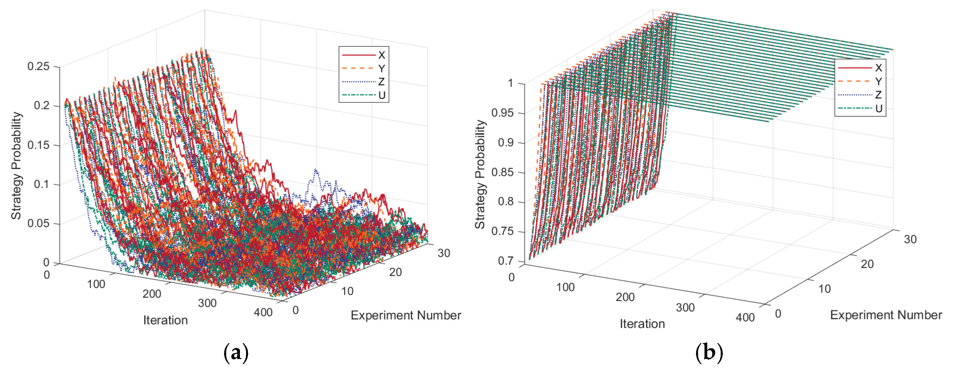
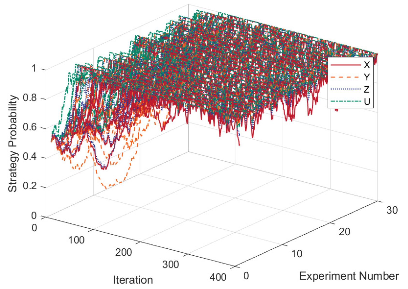
4.2. Validation of Model Credibility and Robustness

Numerical simulation is performed according to the initial parameters, and the base case is illustrated in Figure 5, where the game model evolves toward (1, 1, 1, 1). The initial parameters satisfy  { ( X 3 X 4 ) Y 2 Z 2 U 2 } . According to the model analysis, at this point, the system’s steady state is (1, 1, 1, 1). This aligns with the model analysis, confirming its validity and the credibility of the simulation experiment. Strategy probabilities x, y, z, and u converge to 1 in iterations 85, 70, 67, and 46, respectively, with convergence rates of approximately 0.006, 0.007, 0.007, and 0.011. They have means of 0.90, 0.91, 0.92, and 0.96, along with standard deviations of 0.17, 0.19, 0.16, and 0.11, respectively. The game system is stable, and U evolves significantly faster than the other three.
Thirty repeated experiments were conducted to verify the system’s robustness. The results and numerical indicators are presented in Figure 6 and Table 7. The system’s final evolution was consistent across experiments, with similar convergence paths for each subject. In each experiment, the mean, median, and standard deviation of strategy probabilities for each agent were not significantly different, confirming the model’s robustness. Subsequent simulations were also repeated multiple times, yielding regular results that ensured the reliability of the findings.

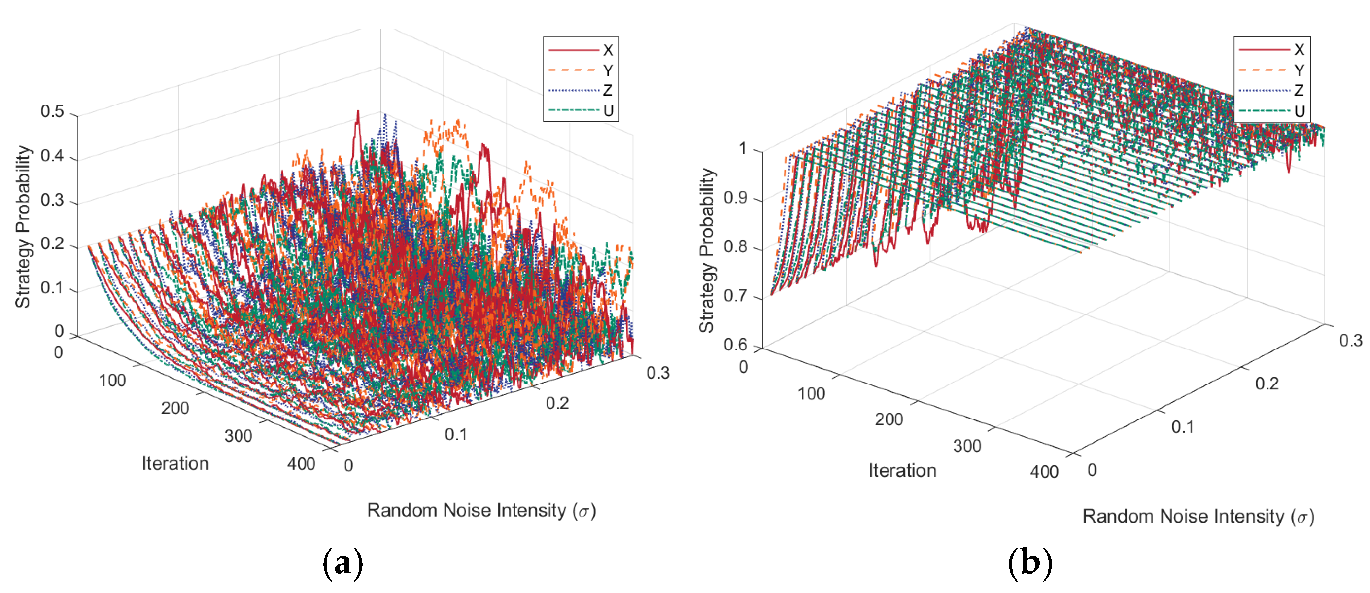
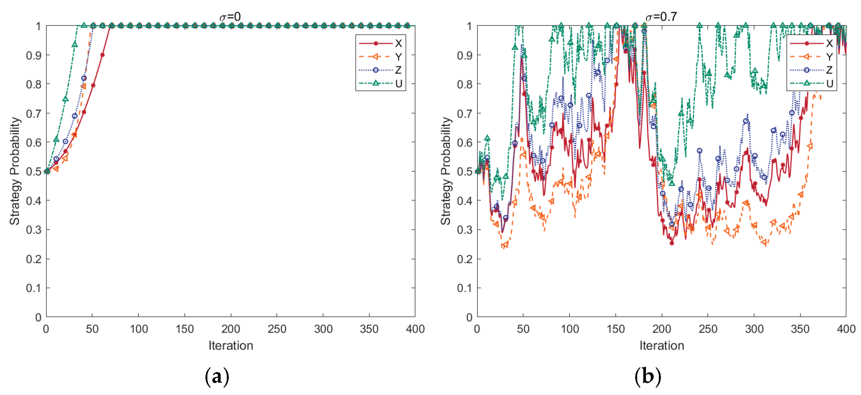
4.3. Effects of Stochastic Perturbations

The evolutionary paths of the parties under different random perturbation intensities are shown in Figure 7. In the absence of random perturbation factors ( σ = 0 ), the strategy probabilities of X, Z, Y, and U converge to 1 after 69, 53, 48, and 34 iterations, respectively. The slopes of the curves reflect the evolutionary rates, which are 0.007, 0.009, 0.010, and 0.015, respectively. Compared with the base case (Figure 5), in the absence of random perturbation factors ( σ = 0 ), the evolutionary paths of the agents are more stable and evolve more quickly. When the value of random perturbation increases ( σ = 0.7 ), the strategy probability changes significantly, and the times for the first x, y, z, and u to stably converge to 1 are 156, 142, 148, and 82, respectively. The mean values of x, y, z, and u are 0.57, 0.50, 0.65, and 0.84, respectively, while standard deviations are 0.20, 0.23, 0.21, and 0.17, respectively. Compared with the base case (Figure 5), the mean value decreases and the standard deviation increases. This indicates that the system is unstable when the external environment changes drastically, and the group’s willingness to reduce emissions is not high. Starting from the initial fluctuation, the system reaches (1, 1, 1, 1) for the first time after approximately 156 iterations. When the system iterates about 370 times, it reaches the stable state of (1, 1, 1, 1) for the second time, which indicates that the system is robust and the PBSC has some adaptability. In either case, the Dismantling and Recycling Party (U) reaches the steady state first and is least affected by random disturbance factors.

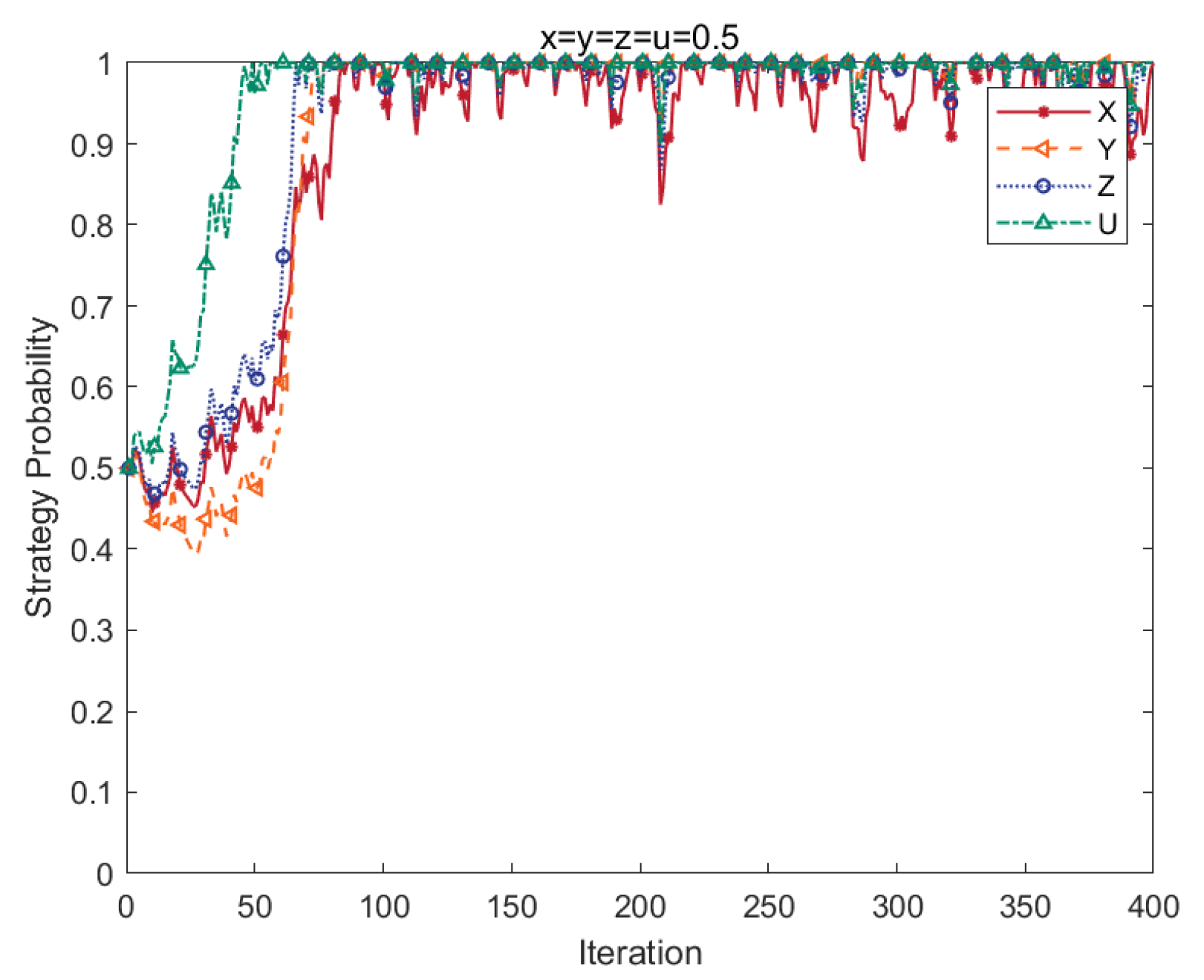
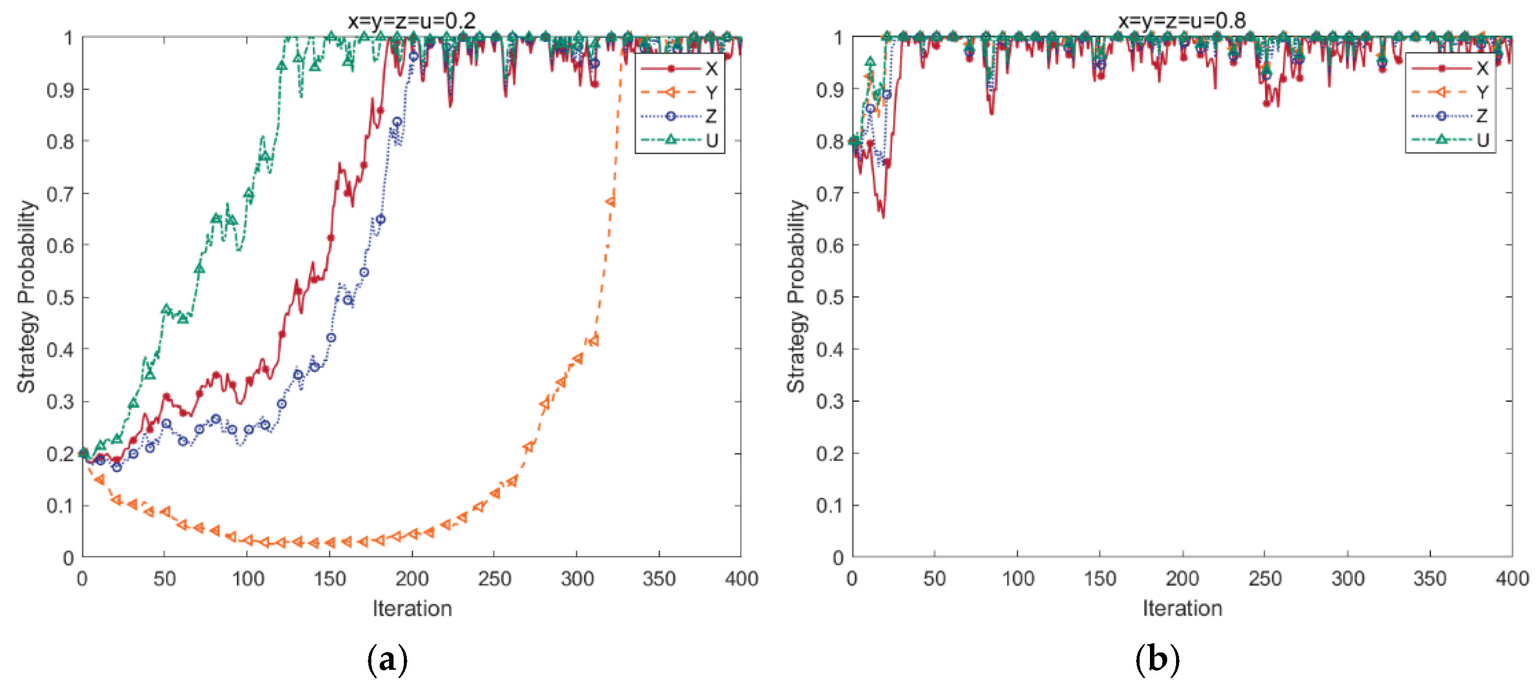
4.4. Effects of Strategy Probability

The evolution paths of the parties under different strategy probabilities are shown in Figure 8. In the case of low strategy probability (Figure 8a), the iterations of x, y, z, and u converging to 1 are 186, 329, 201, and 126, respectively. Among them, y converges to 0 151 times before converging to 1, with the inflection point at (151, 0.03). The means of the probabilities of the X, Y, Z, and U strategies are 0.71, 0.29, 0.67, and 0.84, while standard deviations are 0.31, 0.36, 0.35, and 0.26, respectively. In the case of high strategy probability (Figure 8b), the iteration times of x, y, z, and u finally converging to 1 are 33, 25, 21, and 21, respectively. The X, Y, Z, and U strategy probabilities mean 0.96, 0.99, 0.98, and 0.99, with standard deviations of 0.06, 0.03, 0.05, and 0.03, respectively. Increasing the strategy probability significantly accelerates the system evolution, especially for Y. In addition, comparing Figure 5, Figure 7 and Figure 8 reveals that increasing the strategy probability is more effective in accelerating system evolution than reducing random disturbances.

4.5. Sensitivity Analysis

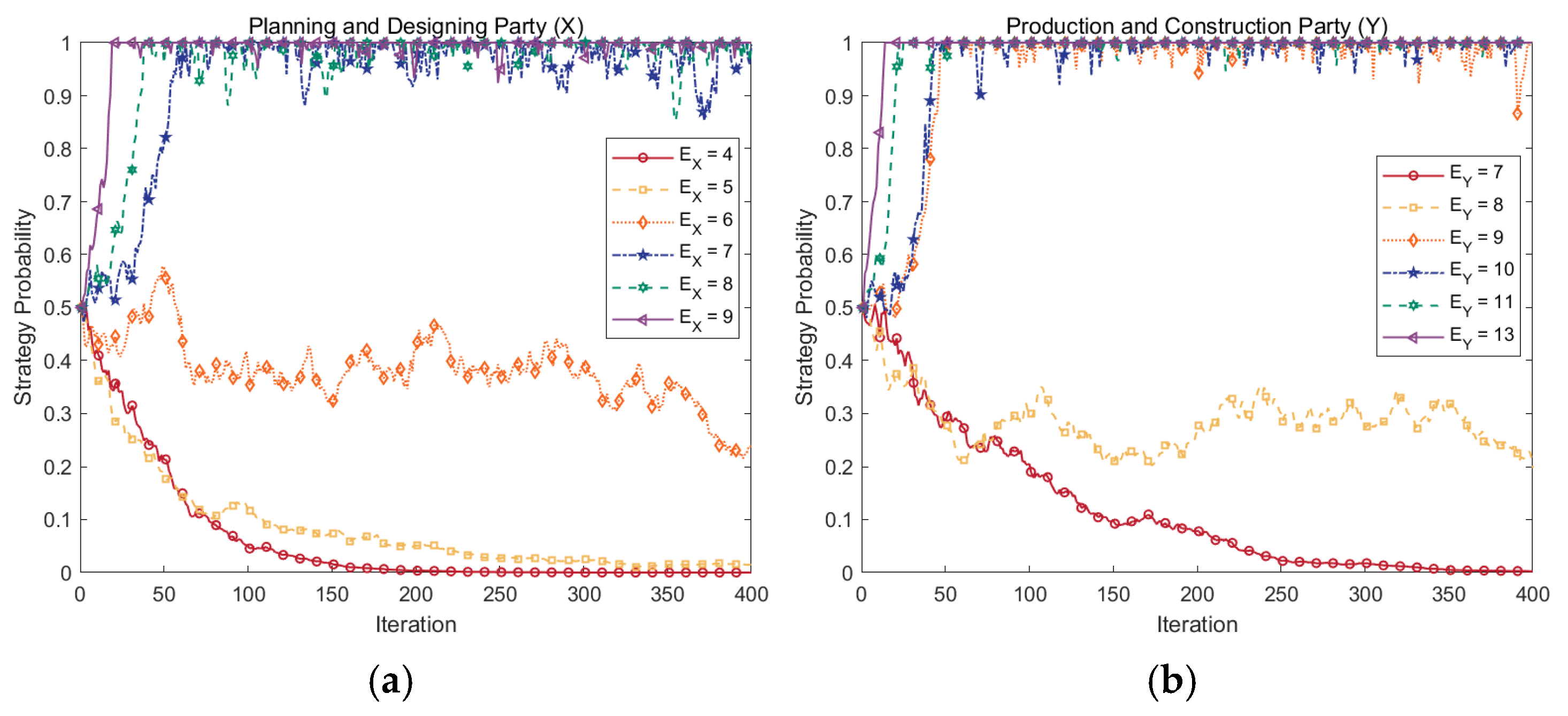
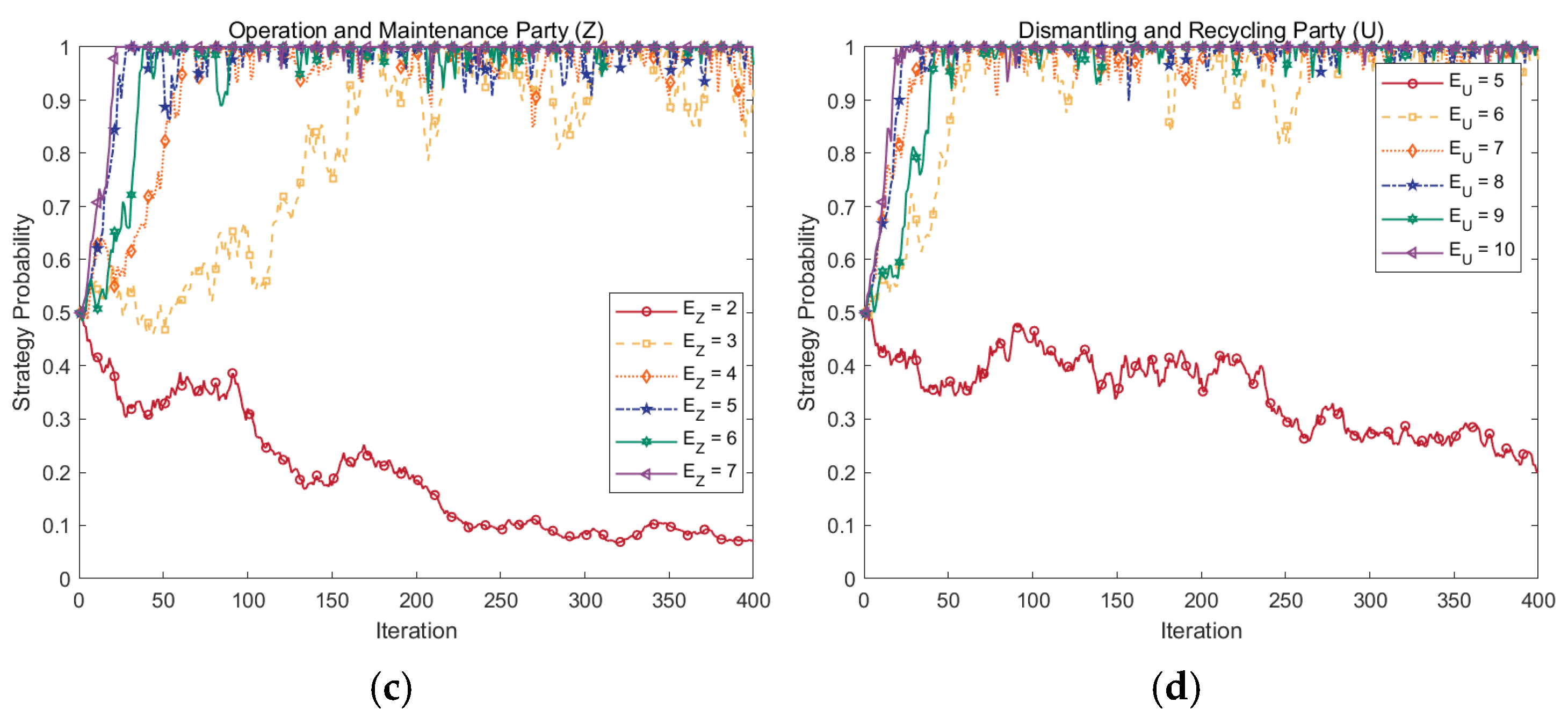
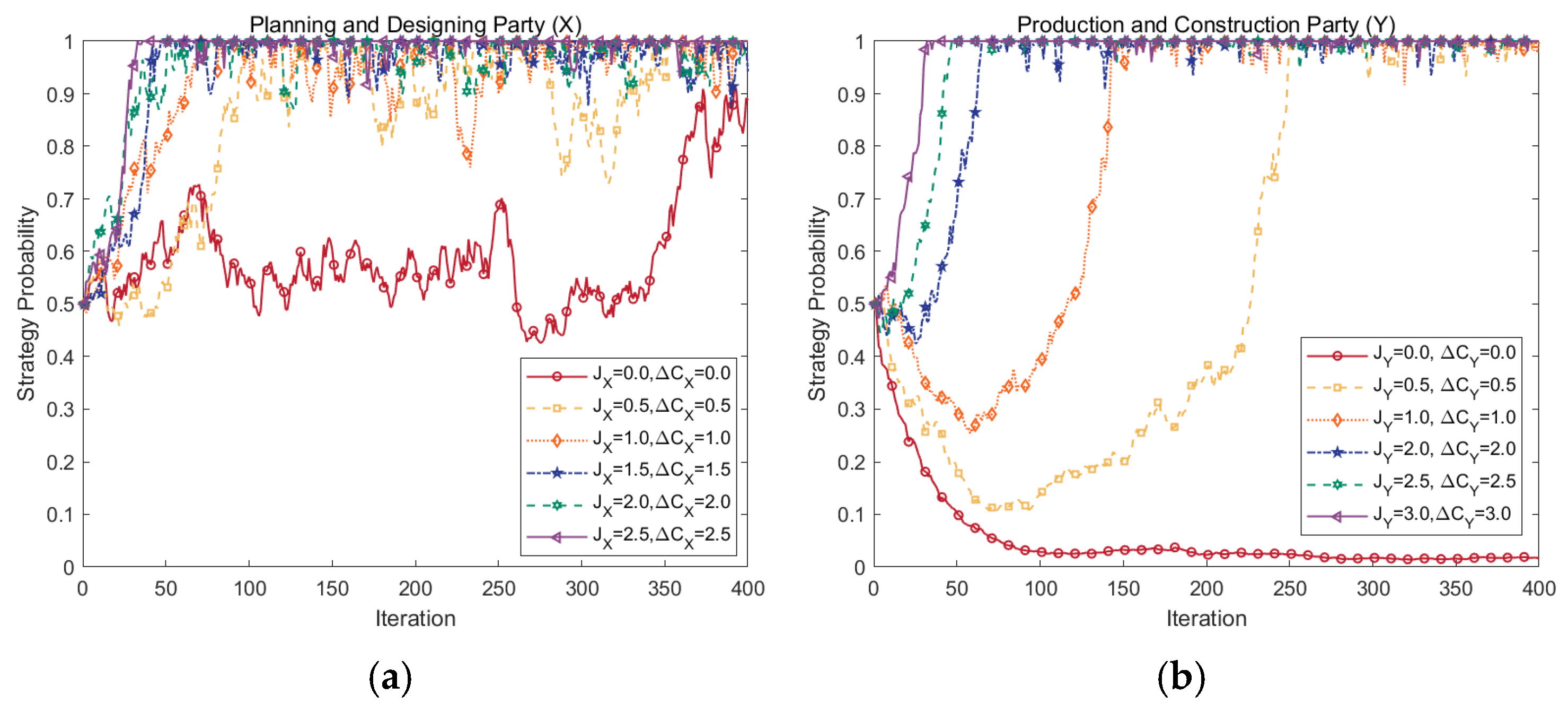
4.5.1. Effects of Abatement Benefits

The evolution of the strategies under different abatement benefits for each agent is shown in Figure 9. The abatement benefits significantly affect the speed and direction of strategy evolution. For the Planning and Designing Party (X), there is a critical value  E X [ 6 , 7 ] , and when  E X E X , x converges to 1, X chooses an “abatement” strategy. Similarly, the critical values of abatement benefits for the Production and Construction Party (Y), Operation and Maintenance Party (Z), and Dismantling and Recycling Party (U) choosing different strategies are  E Y [ 8 , 9 ] , E Z [ 2 , 3 ]  and  E U [ 5 , 6 ] , respectively, with Y being the highest. X is most sensitive to abatement benefits. When  E X  is 7, 8, and 9, the convergence speeds of x to 1 are 0.008, 0.014, and 0.026, respectively. For every 1 increase in  E X , the average increase in evolution speed to the steady state is 0.009, reducing the number of iterations by approximately 20. For the three downstream agents in PBSC, their evolution speed to the steady state will not continue to accelerate with increasing benefits once the abatement benefits reach a critical value of  E Y = 11 , E Z = 6 , E U = 7 . In this case, the convergence rates of y, z, and u to 1 are 0.021, 0.019, and 0.023, respectively.

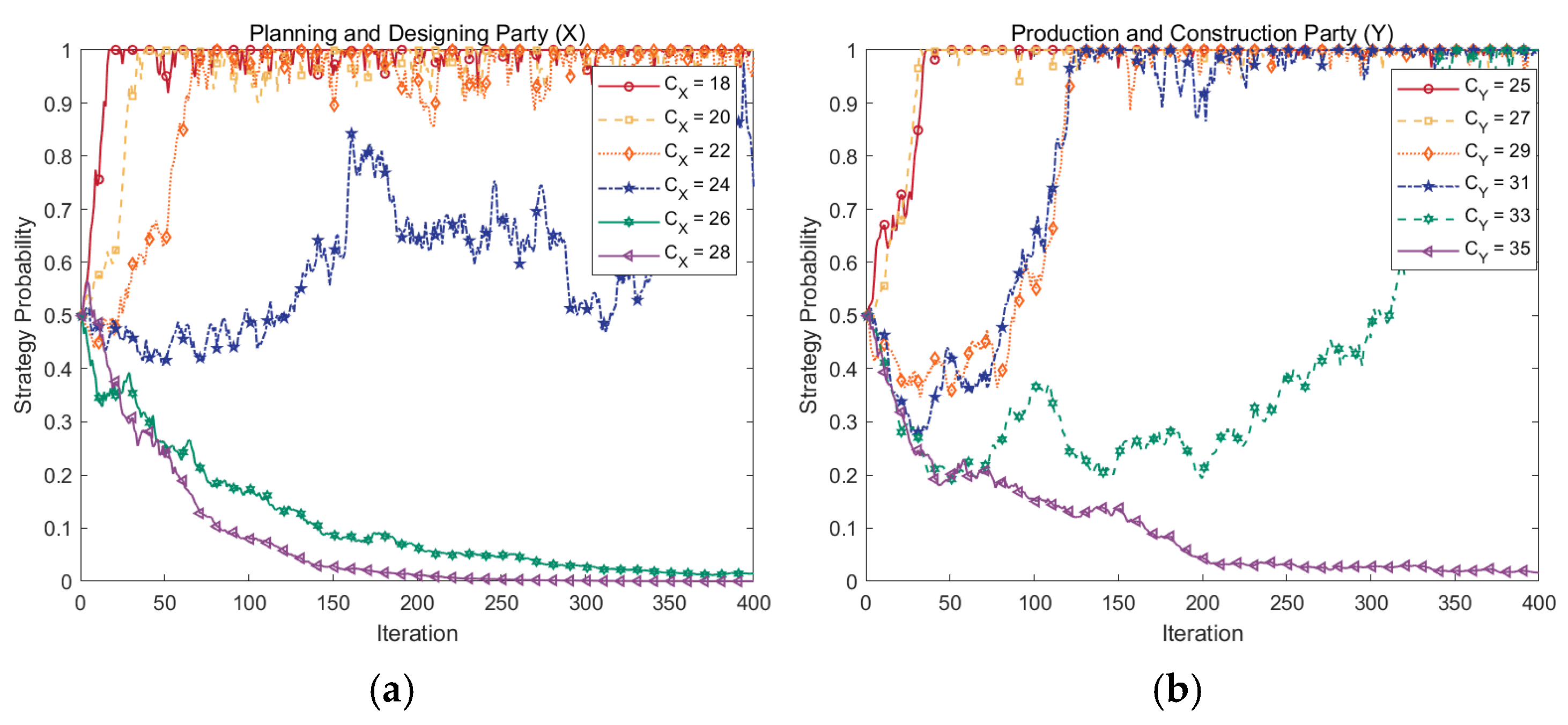
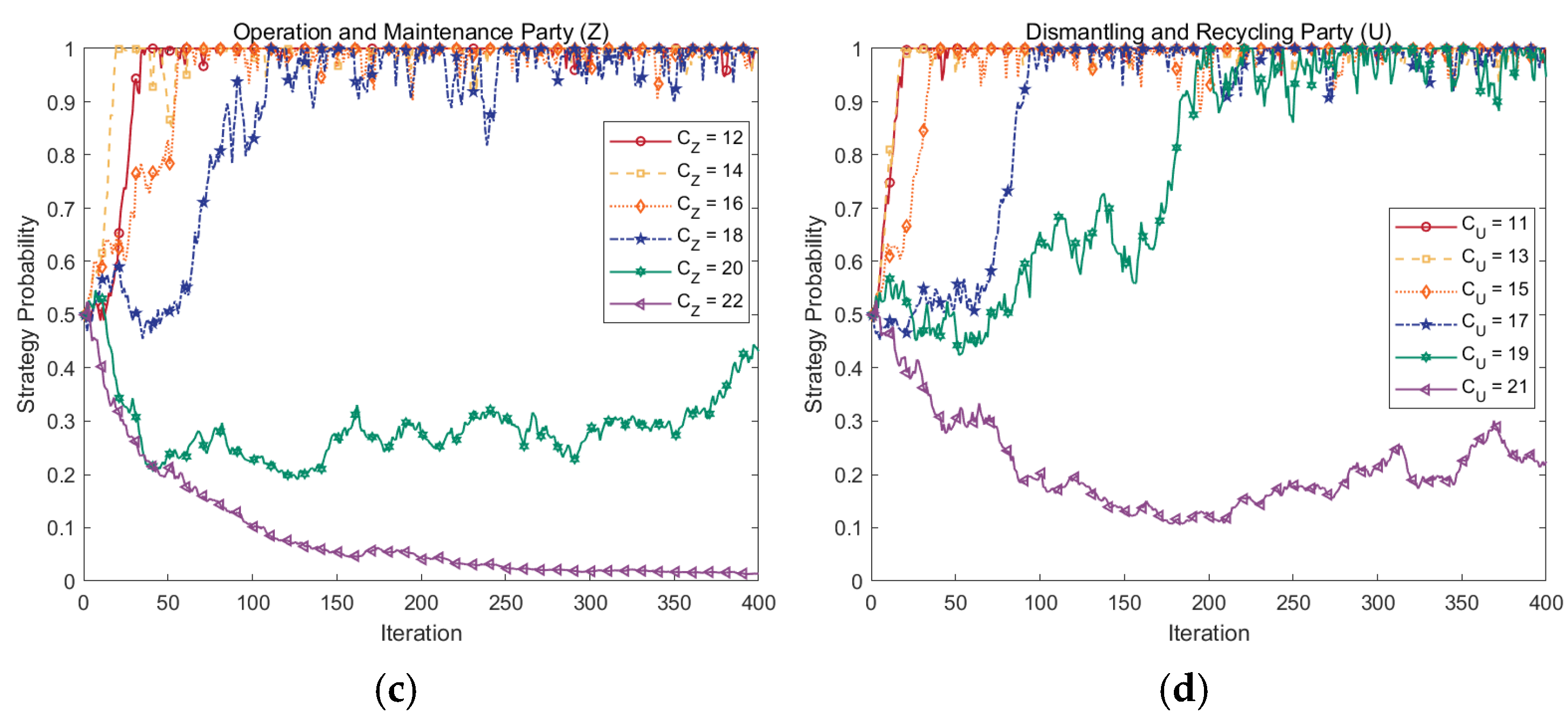
4.5.2. Effects of Abatement Costs

The evolution of strategies under different abatement costs for each agent is shown in Figure 10. The cost of abatement significantly affects the direction and speed of evolution. For the Planning and Designing Party (X), there is a critical value  C X [ 24 ,   26 ] , and when  C X C X , x converges to 0. When  C X = 24 , x fluctuates continuously within [0.42, 0.82]. When  C X  is 28 and 26, x converges to 0 for 362 and 232, respectively. The larger the value of the deviation, the faster the rate of evolution. Similarly, the critical values of abatement costs for Y, Z, and U choosing different strategies are  C Y [ 33 ,   35 ] , C Z [ 20 ,   22 ] , and  C U [ 19 ,   21 ] , respectively, with Y being the highest. X is the most sensitive to the abatement cost. When  C X  are 18, 20, and 22, x converges to 1 for 17, 35, and 66 iterations, respectively. When  C X C X , the number of iterations for x converges to 1 and decreases by approximately 15–30 for every two decreases. The evolutionary rate will not continue to increase when the abatement cost is reduced to a certain level, with critical values of the costs at  C Y = 27 , C Z = 14 , C U = 13 . In this case, y, z, and u converge to 1 at a rate of approximately 0.014, 0.011, and 0.022, respectively.

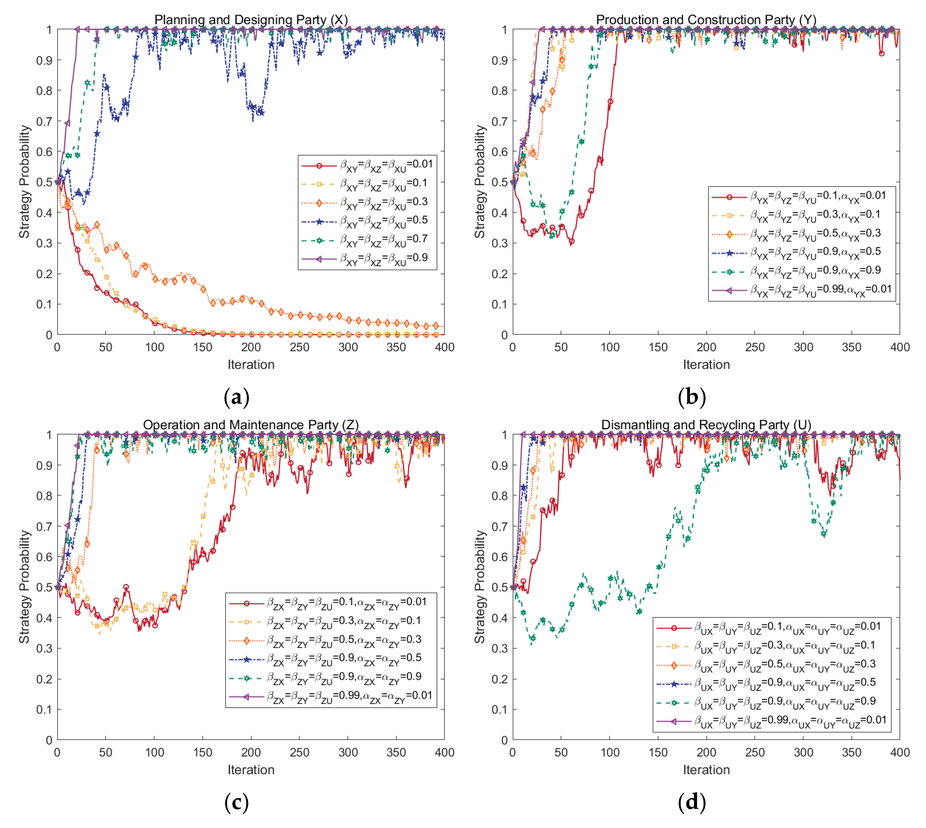
4.5.3. Effects of Information Absorption and Transformation Efficiency

The evolution of strategies under different information absorption and transformation efficiencies of each agent is shown in Figure 11. The absorption and transformation efficiency reflects the ability to process information in implementing carbon abatement strategies, and the greater the ability, the more inclined to choose the “abatement” strategy. The Planning and Designing Party (X) is the most sensitive. When  γ X λ X = 0.02 , after 70 iterations for x, the stabilization fluctuation is at [0.20, 0.39]. When  γ X λ X = 0.08 , x converges to 1 after 262 iterations. When  γ X λ X [ 0.4 ,   0.6 ] , x converges to 1 at a rate of 0.005–0.009. When  γ X λ X = 1.8 , x converges rapidly to 1 at a rate of 0.031. For Y and Z, when the information processing capacity is too poor, Y and Z first converge towards 0 before shifting to converge towards 1 as the effect accumulates, with inflection points of (95, 0.16) and (137, 0.22), respectively. And u always converge to 1, with an evolutionary speed between 0.004 and 0.03. Increasing the information processing capacity does not affect U’s strategy selection direction and only speeds up the evolution.

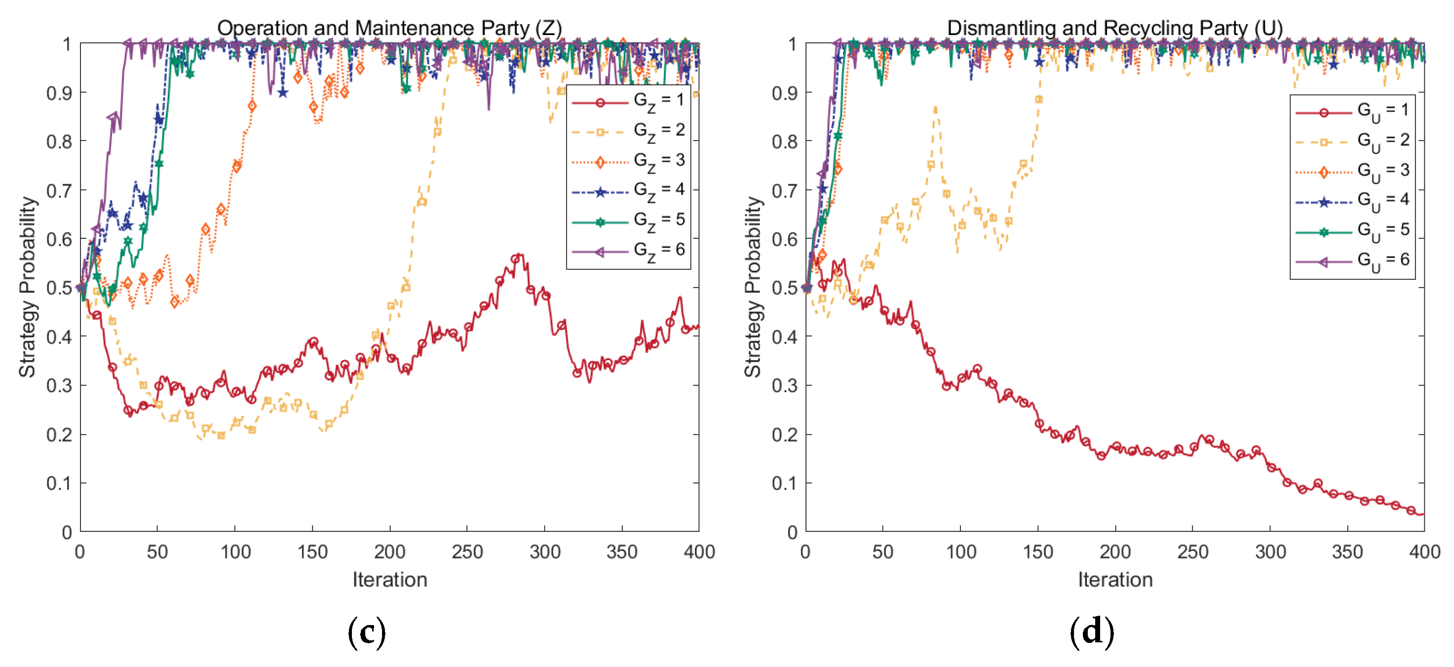
4.5.4. Effects of Joint Abatement Benefit Coefficients and Free-Riding Benefit Coefficients

The evolution of agents’ strategies with different joint abatement and free-rider benefit coefficients is shown in Figure 12. PBSC synergy is proportional to the joint abatement benefit coefficient and inversely proportional to the free-rider benefit coefficient; the more significant the synergy of the PBSC, the more the agent chooses the “abatement” strategy. Since the Planning and Designing Party (X) is at the top of the PBSC, it is complex to obtain benefits from downstream abatement agents by free-riding, and it is most sensitive to the response to synergistic capacity, there exists  β X i * [ 0.3 ,   0.5 ] , when  β X i β X i *  and x converges to 1, otherwise it converges to 0.
Since the free-rider benefit coefficient is set to be less than or equal to the joint abatement benefit coefficient, the strategy probabilities of downstream PBSC agents are more inclined to converge toward 1. The larger the difference between the two coefficients, the faster the convergence rate. However, Y and Z converge toward 0 when both synergizing over hitchhiking benefits are low and only begin to converge toward 1 later as the effects accrue. For Y, the inflection points of the two lines are (39, 0.32) (59, 0.31). For Z, the inflection points of the two lines are (55, 0.36) and (86, 0.36). Y is more sensitive to these two indicators. Since the Dismantling and Recycling Party (U) is at the end of the PBSC, it can obtain free-rider benefits from multiple upstream agents. When the joint abatement benefit coefficients and free-riding benefit coefficients are the same, the number of iterations for u to converge to 1 significantly increases to 232. Although the direction of convergence remains the same, the rate of evolution slows down significantly.
The free-riding phenomenon among agents in PBSC creates a mismatch between abatement responsibilities and benefits. The upstream abatement agent’s cost is not shared, but the benefit is. When long-term synergy with other agents is not apparent, or other agents refuse to share abatement responsibilities, the upstream PBSC agent will gradually choose the “no-abatement” strategy. By then, the free-rider effect in PBSC will be profound, reducing the number of agents choosing “abatement” strategies. The gaming system will gradually evolve to the (0, 0, 0, 0) state, which is not conducive to the sustained implementation of abatement strategies.

4.5.5. Effects of Penalties for Non-Compliance

The evolution of strategies under different intensities of default penalties is shown in Figure 13. In the no-regulation case, x and y first converge to 0 and then to 1 after 101 and 69 iterations, respectively; after 211 and 156 iterations, respectively, they stabilize at 1; while z and u keep converging to 1, with rates of 0.004 and 0.010, respectively. In the high-intensity regulation case, x, y, z, and u converge quickly to 1, with iterations of 46, 61, 55, and 49, respectively. However, in the initial stage of evolution, y and z first converge to 0 before shifting towards 1, with inflection points at (26, 0.35) and (22, 0.42), respectively. Compared with the no-regulation (Figure 13a) and base cases (Figure 5), high penalties can significantly shorten the fluctuation interval and markedly increase X’s willingness to implement abatement strategies. High-intensity regulation (Figure 13b) evolves similarly to the no-perturbation case (Figure 7a), suggesting that further increasing regulation intensity will not achieve a significant effect and may even cause conflicts between X and downstream agents, hindering synergistic cooperation.

4.5.6. Effects of External Losses

The strategy evolution under different external losses for each agent is shown in Figure 14. External losses significantly affect the speed and direction of the agent’s evolution and are inversely related to the agent’s willingness to reduce emissions. For the Planning and Designing Party (X), when  G X = 1 , x converges stably to [0.2, 0.3] after 21 iterations. There is a critical value  G X [ 1 ,   2 ] , and when  G X G X , x converges to 1. At the critical value, x converges to 1 in at least 164 iterations. Similarly, the critical values of y, z, and u for convergence to 1 are  G Y [ 2 ,   3 ] , G Z [ 1 ,   2 ]  and  G U [ 1 ,   2 ] , respectively. This indicates that appropriate enhanced monitoring of Y by external regulators can help urge it to implement its abatement strategy proactively. For X, when  G X = 5  and  G X = 6 , x converges to 1 in 39 and 46 iterations, respectively. For X, when  G X G X = 5 , the marginal utility of the external loss stabilizes and continued external pressure on the agent’s non-abatement behavior will have no significant effect and may lead to rent-seeking. Similarly, for Y and U, the critical value of the external loss effectively pushes them to implement an “abatement” strategy of  G Y = 4 , G U = 3 . At this point, y and u converge to 1 for 40 and 30 iterations, respectively.

4.5.7. Effects of External Incentives and Aids

The evolution of strategies under different external incentives and aids for each agent is shown in Figure 15. Both indicators reflect the extent of external support for PBSC agents in implementing abatement strategies and are directly proportional to the agents’ evolution speed towards abatement. Y is most sensitive to these two indicators. When these two metrics are 0, y converges toward 0, reaching 0.03 after 103 iterations and approaching 0 after 241. When the two indicators are not 0, y is converged to 1, but the number of iterations is different: when  J Y = 0.5 , Δ C Y = 0.5 , to iterate 250 times; when J Y = 1.0 , Δ C Y = 1.0 , to iterate 144 times; when J Y = 2.0 , Δ C Y = 2.0 , to iterate 63 times. In all three cases, y converges to 0 at the beginning and then to 1, with inflection points (93, 0.11), (61, 0.27), and (26, 0.43). With increasing indicators, y converges to 1 in fewer iterations. When X is not incentivized and helped ( J X = 0 , Δ C X = 0 ), x fluctuates continuously in the interval (0.43, 0.70) for a long time. When these two indicators are not 0, x converges to 1. For Z and U, these indicators only affect the rate of evolution, not the direction. Thus, the focus should be on incentivizing and assisting X and Y.

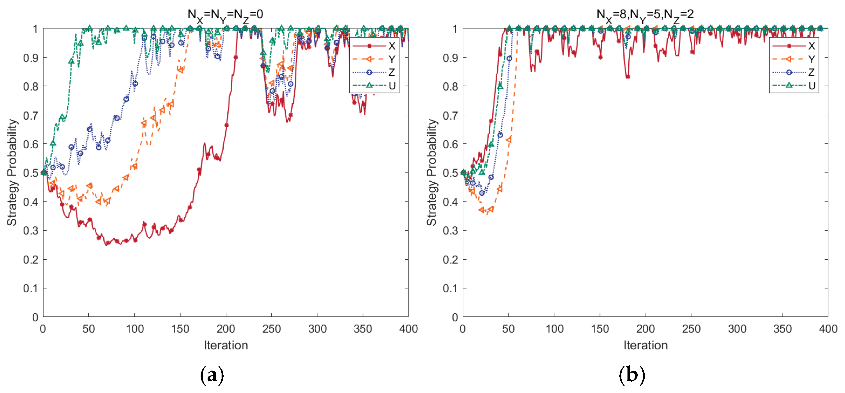
4.5.8. Effects of External Information Content

The evolution of the parties’ strategies under different external information contents is shown in Figure 16. Compared with the base case (Figure 5), when the external information content is low ( D = 1 ), x, z, and u are stabilized to converge to 1 in 372, 356, and 192 iterations, respectively. In this case, y converges initially to 1 with the other agents six times and then to 0, stabilizing at around 0.2 after 19 iterations. This is because Y cannot consistently obtain enough information about emission reduction. Relevant organizations outside the PBSC should strengthen publicity, targeted research, and development of abatement tools and technologies related to the production and construction process, which can effectively promote the absorption and use of Y to achieve high-quality abatement. In contrast, when the external information content is high ( D = 10 ), x, y, z, and u converge to 1 at about 0.007, 0.008, 0.008, and 0.011, respectively. This is better than the base case (Figure 5) and closer to the no-perturbation case (Figure 7a), suggesting that enhanced information sharing can help overcome random perturbations.

5. Discussion

5.1. Summary of Findings

Based on the model analysis and simulation, the results of the study can be summarized in the following five points:
  • Stochastic perturbation factors and initial strategy probability play a significant role in the gaming system’s evolutionary situation. When the environment in which the PBSC operates is unstable, it lengthens the fluctuation interval and significantly reduces the speed of strategy evolution. Increasing the proportion of the initial carbon emission reduction group is more conducive to accelerating the system’s evolution.
  • The agents’ abatement benefits and costs significantly affect the choice of strategy. It is most favorable to promote the abatement strategy when the party’s abatement benefit and cost are at  [ E i , E i ]  and  [ C i , C i ] , respectively. Among them, the Production and Construction Party (Y) is the most sensitive to the benefits and costs of abatement. Consequently, these factors influence Y’s decision to implement abatement strategies.
  • The operational status of the PBSC is a key factor in determining participants’ strategies. X at the top and Y at the bottom of the PBSC are most affected by its synergistic capabilities. Establishing an appropriate monitoring mechanism within the PBSC is conducive to increasing the parties’ willingness to reduce emissions and keeping the penalty for non-compliance to less than twice the amount of the base case is conducive to improving the overall effectiveness of PBSC in reducing emissions.
  • The external environment’s effect on the agents’ strategies is mainly in terms of the losses caused and the help provided. Continued external pressure on Z to reduce emissions can be an effective driver for continued abatement by Z. For other agents, the external loss is within  [ G i , G i ]  to push them to implement abatement strategies. External incentives and aids impact the speed of evolution, most prominently on Y, followed by X. Section 4.5.2, Section 4.5.6, and Section 4.5.7 show that, with other factors constant, equal changes in negative and positive incentives lead to different results: Negative incentives may cause subjects to abandon emission reduction, while positive incentives only affect the system’s convergence speed. External losses are more effective than incentives and aid in promoting emission reduction by agents.
  • The abatement information content is an essential factor affecting decision-making. The information content positively correlates with the agent’s willingness to reduce emissions. It is optimal to keep the information content  D [ 5 , 10 ]  to ensure that each agent implements an abatement strategy and avoids wasting resources. The agent’s ability to process information is positively related to the evolutionary speed. It has the most significant effect on X. When  γ X λ X 0.08 , X rejects abatement.

5.2. Recommendation

In response to the above summary, the following recommendations are made:
  • Maintaining a stable market, increasing the resilience of the PBSC, and increasing the proportion of emission reduction groups. Section 4.3 and Section 4.4 demonstrate that maintaining system stability and enhancing initial emission reduction intentions can facilitate PBSC emission reduction. The consumer market drives, while the supply market supports. To promote the implementation of emission reduction strategies by participants in the PBSC, the following measures should be taken: (1) Enhance public environmental awareness and acceptance of PB to boost consumers’ willingness to pay [29]. (2) As the general organizer, the government should introduce policies to stabilize the market and prices, alleviating construction companies’ concerns over carbon emission reduction [50]. (3) The PBSC should enhance risk resistance through stronger cooperation among participants to better adapt to market changes.
  • Participants in PBSC should reduce costs, increase efficiency, and improve capacity in production, promotion, and co-operation. Section 4.5.1 and Section 4.5.2 indicate that the direct costs and benefits significantly influence enterprises and those engaged in construction should actively participate. The first is to reduce costs via technological innovation and upgrading, corporate R&D cooperation, and construction collaboration [38]. Secondly, use advertising and packaging design to promote emission reduction concepts, expand the market, publicize high-quality projects, and set industry benchmarks to guide more projects to reduce emissions [56]. Thirdly, actively seek opportunities for cooperation [16,37]. For example, reduce employment and training costs via school–enterprise cooperation; lower procurement costs through long-term supplier relationships; decrease R&D costs by collaborating with research institutions; and share resources and complement strengths with peer enterprises via strategic alliances to undertake large-scale projects and achieve standard emission reductions.
  • Enhance the internal communication and information-sharing mechanisms within the PBSC, focusing on participants at both ends of the PBSC, with appropriate external intervention for optimization. Section 4.5.4 highlights that focusing on the beginning and end of PBSC agent, enhancing coordination, and avoiding the “free-rider” effect can promote emission reduction. Enhancing information flow within PBSC promotes collaborative emission reduction, while ensuring information security prevents free riding [83]. PBSC participants should form alliances, enhance communication, and optimize the PBSC operation process [36]. Upstream owners should initiate the establishment of an information-sharing platform. Downstream end-user enterprises should actively respond to enhance PBSC synergy, increase joint abatement benefits, and mitigate the adverse impact of free-rider behavior [17]. The information-sharing platform should adopt the following optimization measures: (1) Use API, EDI, and other real-time data exchange technologies to realize real-time data transmission and update and enhance PBSC synergy. (2) Employ firewalls, intrusion detection, and defense systems to enhance privacy protection, ensure data security, and prevent free-riding by downstream participants. (3) Establish a project-centric information-sharing database, reduce information redundancy through standardized design, and enhance collaboration efficiency. The government, industry associations, and other entities can intervene in the PBSC to guide the establishment of a cost-compensation mechanism, optimize the benefit-distribution mechanism, reduce free-riding, and enhance participants’ enthusiasm for emission reduction [41].
  • External parties in PBSC should insist on punishment over reward and adopt differentiated instruments. Negative incentives play a significant role in reducing emissions. Section 4.5.6 and Section 4.5.7 reveal that external incentives, whether positive or negative, significantly impact PBSC emission reduction. By strengthening regulatory measures from governments and environmental agencies [50], enhancing consumer awareness of green products, and increasing costs for non-compliant participants, losses can be amplified to compel the main parties to reduce emissions. The focus is on enterprises involved in operation and maintenance. Positive incentives should be targeted at the planning, design, production, and construction stages [4,11,17], with the following measures adopted: (1) The government can reduce uncertainty by introducing supportive policies, guiding public opinion, and providing financial subsidies. (2) The market is the environment for PBSC operation. Stable and orderly building materials, carbon trading, and talent markets facilitate smooth PBSC operations, lower participants’ perceived emission reduction risks, and reduce reserved risk-mitigation costs. (3) Colleges, universities, banks, tech firms, etc., should collaborate via joint training and research, and lower financing thresholds, to help PBSC participants overcome difficulties and promote emission reductions.
  • Establish a cross-industry information-sharing platform to optimize PBSC’s information-sharing mechanism and enhance participants’ information processing capabilities [56]. Section 4.5.3 and Section 4.5.8 indicate that both the agent’s information processing capacity and the environmental information content are crucial for PBSC emission reduction. Governments and industry associations should take the lead in establishing a cross-departmental comprehensive information sharing platform, integrating market dynamics, policies, regulations, and technological progress, and breaking information silos. In addition, the platform should actively optimize the information sharing mechanism to reduce participants’ difficulty in collecting and using: (1) Develop harmonized standards to ensure accurate and reliable information. (2) Establish an incentive system to encourage units to share information through financial support, co-operation opportunities, etc. (3) Adopt advanced technologies like cloud computing, big data, IoT, and blockchain to enhance the efficiency and accuracy of information sharing. Within the PBSC, the BIM platform and carbon dashboard can provide digital project information and monitor carbon emissions in real time [84]. They can also link with external information platforms to attract more enterprises to participate in information sharing, increase transparency, and enable participants to obtain personalized information. PBSC participants should enhance their emission reduction awareness, actively seek related technologies, knowledge, and information, establish a professional information analysis team to collect and analyze market-related emission reduction information and feedback from other entities, providing a scientific basis for decision-making, and conduct staff training to improve emission reduction awareness and information processing capabilities, thereby increasing benefits [38].

6. Conclusions

Considering that the PBSC faces many internal and external uncertainties, Gaussian white noise is introduced to simulate random perturbation factors, and a four-way stochastic evolutionary game model is constructed to abate carbon emissions among the participants of the PBSC. Subsequently, using MATLAB software, numerical simulation was carried out to summarize the five aspects of stochastic perturbation factors, participants’ ability to reduce emissions, PBSC operating conditions, the PBSC external environment, and abatement information, to make targeted recommendations. The contributions and shortcomings of the study are as follows.

6.1. Implications

Academics acknowledge the crucial role of PBs in reducing carbon emissions in the construction industry and the significant contributions of PBSC participants involved in design, construction, and operation. However, there has been limited examination of the relationships between participants in the full PBSC regarding strategy implementation. This study differs from previous ones by not only examining the impact of external interventions on decision-making but also considering the interactions among various PBSC participants in implementing abatement strategies. Furthermore, stochastic perturbation factors undoubtedly impact participants’ decision-making in the PBSC, yet few studies have analyzed decision-making in this context. This study analyses the impact of each parameter on the change in each participant’s strategy in the context of stochastic perturbation to bring the conclusions closer to reality.
The model’s parameter setting considers stochastic perturbation factors, participants’ capabilities, PBSC synergy status, external agencies’ behavior, and environmental information, with conclusions drawn through simulation, offering insights into promoting participants’ emission reductions, optimizing the PBSC, and innovating management models. At the same time, it can provide suggestions for PBSC participants, such as contractors, builders, and operators, to respond to external changes and choose strategies. It can also serve as a decision-making basis for external organizations such as governments, financial institutions, and universities.
In conclusion, this study expands the research scope on implementing carbon reduction strategies by PBSC participants, offers a modeling framework for studying PBSC, and provides insights into carbon reduction and supply chain construction for PBs. It also inspires decision-making by both participants and external organizations.

6.2. Limitations

This study explores the intrinsic mechanisms of carbon reduction strategies implemented by PBSC participants through a four-way stochastic evolutionary game model. However, the following limitations remain: (1) The PBSC is long and has many participants. The study categorizes the many participants based on typical characteristics of each group, while ignoring individual differences among participants. Adjusting parameters and models can further refine the analysis of specific participants. (2) The long life cycle of PBs makes it difficult to find a case with a complete PBSC for numerical simulation in practice. Though the parameters encompass most PBSC emission reduction scenarios, real-world complexities may introduce extreme or exceptional scenarios beyond this range. Therefore, the parameters set in this paper are idealized, based on reality, policy references, and relevant literature. As PBSC evolves, parameters can be refined and extended to address specific cases, enhancing realism.
In addition, the model constructs a framework for studying the impact of emission reduction strategies of PBSC participants, how to further optimize the model to make it more realistic, and specific needs to be continued in further research. This study’s stochastic four-way evolutionary game model is expected to provide ideas for related research.

6.3. Future Work

In the future, real cases could be used for analysis. Adjusting the model and parameters to the company’s specific characteristics will improve the applicability of the simulation results. The unique characteristics of specific PB projects can be considered to extend the parameter range. The operation mechanism of PBSC is uniform across countries, which makes this model applicable. However, national conditions, cultures, and policies vary from country to country. For example, Europe’s ETS indirectly interacts with enterprises through the carbon market through the cap-and-trade mechanism. Tax credits in the United States directly encourage enterprises to develop low-carbon technologies [85]. Therefore, it is necessary to modify the model appropriately for practical application.
Digital twin technology is expected to become an essential direction of PBSC carbon emission reduction research. Digital twins have the functions of real-time monitoring, analysis, and optimization [86]. Real-time monitoring, analysis, and prediction of PB carbon emissions can be realized by integrating digital twins, BIM, and carbon dashboards. This integration will improve the PBSC synergy potential and the overall carbon emission reduction effect by providing dynamic information for all PBSC stages, linkages, and enterprises.
Given the complexity of PBSC and environmental uncertainty, real-world dynamics and agent interactions are far more complex than the random disturbances considered in this context. Thus, a hybrid game–agent model is a promising future research direction. By combining reinforcement learning and game theory, this model can simulate more complex scenarios and deeply explore the intricate relationships among PBSC participants in carbon emission reduction decisions.

Author Contributions

Conceptualization, writing, and original draft preparation were carried out by H.W., L.L., C.G. and R.Z. Methodology, software, review, writing, and editing were carried out by H.W. Supervision was carried out by L.L. All authors have read and agreed to the published version of the manuscript.

Funding

This research was funded by the Liaoning Province social science planning fund, grant number L22BGL042.

Institutional Review Board Statement

Not applicable.

Informed Consent Statement

Not applicable.

Data Availability Statement

Data for this study are available upon request to the corresponding author.

Conflicts of Interest

The authors declare no conflicts of interest.

Abbreviations

The following abbreviations are used in this manuscript:
PBSCPrefabricated Building Supply Chain
PBPrefabricated Building
XPlanning and Designing Party
YProduction and Construction Party
ZOperation and Maintenance Party
UDismantling and Recycling Party

Appendix A

Appendix A.1. Existence and Uniqueness Proof

Prove the existence and uniqueness of solutions of Equations (8)–(11) according to the following theorem.
Theorem A1. 
For  d ( x ) t = f ( t , x ( t ) ) d t + g ( t , x ( t ) ) d w ( t ) , t J , Let the functions  f ( t , x )  and  g ( t , x )  satisfy the following conditions in  J × R d . (i) Consistent Lipschitz conditions. (ii) Linear growth condition [68].
For Equations (8)–(11), since  x [ 0 , 1 ] , y [ 0 , 1 ] , z [ 0 , 1 ] , u [ 0 , 1 ] , t > 0 , only the local Lipschitz conditions and nonlinear conditions need to be satisfied. The proof is as follows:
Write Equations (8)–(11) as Equations (A1)–(A4), respectively:
d x t = f 1 ( x , t ) d t + g 1 ( x , t ) d w t
d y t = f 2 ( y , t ) d t + g 2 ( y , t ) d w t
d z t = f 3 ( z , t ) d t + g 3 ( z , t ) d w t
d u t = f 4 ( u , t ) d t + g 4 ( u , t ) d w t
The individual Equations are expanded as follows:
f 1 ( x , t ) = x [ ( 1 + y β X Y + z β X Z + u β X U ) E X C X + Π X + ( 1 y ) N Y + ( 1 z ) N Z + ( 1 u ) N U + G X ] g 1 ( x , t ) = σ x
f 2 ( y , t ) = y [ ( 1 + x β Y X + z β Y Z + u β Y U x α Y X ) E Y C Y + Π Y + G Y + x N Y ] g 2 ( y , t ) = σ y
f 3 ( z , t ) = z [ ( 1 + x β Z X + y β Z Y + u β Z U x α Z X y α Z Y ) E Z C Z + Π Z + G Z + x N Z ] g 3 ( z , t ) = σ z
f 4 ( u , t ) = u [ ( 1 + x β U X + y β U Y + z β U Z x α U X y α U Y z α U Z ) E U C U + Π U + G U + x N U ] g 4 ( u , t ) = σ u
Clearly, Equations (A5)–(A8) are continuous on  x [ 0 , 1 ] , y [ 0 , 1 ] , z [ 0 , 1 ] , u [ 0 , 1 ] .
First, prove for Equation (8) that it has a local Lipschitz condition:
Equation (A9) holds for  x , x * [ 0 , 1 ] .
f 1 ( x , t ) f 1 ( x * , t ) = [ ( 1 + y β X Y + z β X Z + u β X U ) E X C X + Π X + ( 1 y ) N Y + ( 1 z ) N Z + ( 1 u ) N U + G X ] ( x x * ) [ ( 1 + y β X Y + z β X Z + u β X U ) E X C X + Π X + ( 1 y ) N Y + ( 1 z ) N Z + ( 1 u ) N U + G X ] x x *
Let  K 1 = ( 1 + y β X Y + z β X Z + u β X U ) E X C X + Π X + ( 1 y ) N Y + ( 1 z ) N Z + ( 1 u ) N U + G X  and  K 1  be a positive constant to obtain  f 1 ( x , t ) f 1 ( x * , t ) K 1 x x *
And  g 1 ( x ) g 1 ( x * ) = σ x σ x * σ x x * .
Therefore, Equation (A10) holds.
f 1 ( x , t ) f 1 ( x * , t ) + g 1 ( x ) g 1 ( x * ) = [ ( 1 + y β X Y + z β X Z + u β X U ) E X C X + Π X + ( 1 y ) N Y + ( 1 z ) N Z + ( 1 u ) N U + G X ] ( x x * ) + σ x σ x * [ ( 1 + y β X Y + z β X Z + u β X U ) E X C X + Π X + ( 1 y ) N Y + ( 1 z ) N Z + ( 1 u ) N U + G X ] x x * + σ x x * = { [ ( 1 + y β X Y + z β X Z + u β X U ) E X C X + Π X + ( 1 y ) N Y + ( 1 z ) N Z + ( 1 u ) N U + G X ] + σ } x x *
Let K satisfy Equation (A11)
K = K 1 + σ = [ ( 1 + y β X Y + z β X Z + u β X U ) E X C X + Π X + ( 1 y ) N Y + ( 1 z ) N Z + ( 1 u ) N U + G X ] + σ
Therefore,  f 1 ( x , t ) f 1 ( x * , t ) + g 1 ( x ) g 1 ( x * ) K x x * . Equation (8) satisfies the local Lipschitz condition.
The second proof of the linear growth stability of Equation (8):
From the preceding, Equation (A12) is obtained.
f 1 ( x , t ) 2 = [ ( 1 + y β X Y + z β X Z + u β X U ) E X C X + Π X + ( 1 y ) N Y + ( 1 z ) N Z + ( 1 u ) N U + G X ] x 2 = [ ( 1 + y β X Y + z β X Z + u β X U ) E X C X + Π X + ( 1 y ) N Y + ( 1 z ) N Z + ( 1 u ) N U + G X ] 2 x 2 [ ( 1 + y β X Y + z β X Z + u β X U ) E X C X + Π X + ( 1 y ) N Y + ( 1 z ) N Z + ( 1 u ) N U + G X ] 2 ( 1 + x 2 ) = K 2 ( 1 + x 2 ) g 1 ( x ) 2 = σ x 2 = σ 2 x 2 σ 2 ( 1 + x 2 )
From Equation (A12), Equation (A13) can be obtained.
f 1 ( x , t ) 2 + g 1 ( x ) 2 = [ ( 1 + y β X Y + z β X Z + u β X U ) E X C X + Π X + ( 1 y ) N Y + ( 1 z ) N Z + ( 1 u ) N U + G X ] x 2 + σ x 2 = [ ( 1 + y β X Y + z β X Z + u β X U ) E X C X + Π X + ( 1 y ) N Y + ( 1 z ) N Z + ( 1 u ) N U + G X ] 2 x 2 + σ 2 x 2 [ ( 1 + y β X Y + z β X Z + u β X U ) E X C X + Π X + ( 1 y ) N Y + ( 1 z ) N Z + ( 1 u ) N U + G X ] 2 ( 1 + x 2 ) + σ 2 ( 1 + x 2 ) = ( K 1 2 + σ 2 ) ( 1 + x 2 ) ( K 1 + σ ) 2 ( 1 + x 2 ) = K 2 ( 1 + x 2 )
Since  K 1 0 f 1 ( x , t ) 2 + g 1 ( x ) 2 = ( K 1 2 + σ 2 ) ( 1 + x 2 ) ( K 1 + σ ) 2 ( 1 + x 2 ) = K 2 ( 1 + x 2 ) .
Therefore, Equation (8) satisfies the linear growth condition.
Since initially  t = 0  and  x ( t ) = 0 , at this point, Equation (8) is independent of the Brownian motion.
Therefore, there exists a unique solution to Equation (8).
Similarly, it can be obtained that there exists a unique solution to Equations (9)–(11), which can be analyzed for stability.

Appendix A.2. Stability Condition Derivation

Derive the stability condition from Theorem 1. The derivation of Equation (13) proceeds as follows:
To show that the expected moments of the zero solution are exponentially stable, it is sufficient to show that  L V ( t , x ) μ V ( t , x ) , t 0 .
First, since  x [ 0 , 1 ]  and Equation (8) is a simple linear Equation.
Thus, making  V t ( t , x ) = x , x [ 0 , 1 ] , gives  V t = 0 , V x = 1 , 2 V x 2 = 0 .
When  x 0 V t ( t , x ) 0 ; when  x = 0 V t ( t , 0 ) = 0 .
Therefore  V t ( t , x ) = x , x [ 0 , 1 ]  is positive definite. This is the basis for stability analysis.
It is only necessary to verify  L V ( t , x ) . If  L V ( t , x )  is negative definite or semi-negative definite, then the system is stable at the equilibrium point.
L V ( t , x ) = V t + V x f 1 ( x , t ) + 1 2 2 V x 2 g 1 ( x , t ) 2 = [ ( 1 + y β X Y + z β X Z + u β X U ) E X C X + Π X + ( 1 y ) N Y + ( 1 z ) N Z + ( 1 u ) N U + G X ] x
According to the zero-solution P-order moment-index stabilization condition in Theorem 1, if the lower is stabilized,  L V ( t , x ) μ V ( t , x )  must also be satisfied.
Thus, to satisfy Equation (A15)
L V ( t , x ) 0 L V ( t , x ) μ V ( t , x ) = μ x
Since  x [ 0 , 1 ] , it is only necessary to satisfy the Equation (A16)
L V ( t , x ) = [ ( 1 + y β X Y + z β X Z + u β X U ) E X C X + Π X + ( 1 y ) N Y + ( 1 z ) N Z + ( 1 u ) N U + G X ] x μ x
That is  ( 1 + y β X Y + z β X Z + u β X U ) E X C X + Π X + ( 1 y ) N Y + ( 1 z ) N Z + ( 1 u ) N U + G X 1 , which is Equation (17).
Similarly, Equations (18)–(20) can be derived.
Then, derive the stabilization conditions, using X1 and X2 as examples.
The approximate reduction process of Equation (17) is shown in Equation (A17)
( 1 + y β X Y + z β X Z + u β X U ) E X C X + Π X + ( 1 y ) N Y + ( 1 z ) N Z + ( 1 u ) N U + G X = ( 1 + z β X Z + u β X U ) E X C X + Π X + N Y + ( 1 z ) N Z + ( 1 u ) N U + G X + y ( β X Y E X N Y ) 1 y ( β X Y E X N Y ) 1 ( 1 + z β X Z + u β X U ) E X + C X Π X N Y ( 1 z ) N Z ( 1 u ) N U G X
A categorical discussion of  ( β X Y E X N Y )  yields the conditions for satisfying Equation (A17) as
X1. 
When  x ( 0 , 1 ]  and  β X Y E X N Y > 0 y 1 ( 1 + z β X Z + u β X U ) E X + C X Π X N Y ( 1 z ) N Z ( 1 u ) N U G X / ( β X Y E X N Y )  and  0 1 ( 1 + z β X Z + u β X U ) E X + C X Π X N Y ( 1 z ) N Z ( 1 u ) N U G X  should be satisfied.
X2. 
When  x ( 0 , 1 ]  and  β X Y E X N Y < 0 y [ 1 ( 1 + z β X Z + u β X U ) E X + C X Π X N Y ( 1 z ) N Z ( 1 u ) N U G X ] / ( β X Y E X N Y )  and  1 ( 1 + z β X Z + u β X U ) E X + C X Π X N Y ( 1 z ) N Z ( 1 u ) N U G X 0  should be satisfied.
Similarly, it can be deduced that Y1, Z1, and U1 hold.
Similarly, it can be deduced that Equations (21)–(24) hold and it can be shown that the conditions X3, X4, Y2, Z2, and U2 hold.

Appendix B. Expert Interview Process

In this study, semi-structured interviews were conducted. Questions were posed flexibly based on the interview outline, allowing an in-depth grasp of the experts’ views. The research centered on PBSC carbon emission reduction, examining the experts’ consensus on both the basis of parameter setting and the parameter setting itself. The interviews aimed to verify the basis’ reliability and the parameter setting’s scientific nature.
We interviewed experts from both universities and enterprises. University experts provided theoretical insights, while enterprise experts shared practical views on PBSC emission reduction. Their suggestions confirmed the parameter basis’s reliability and the parameter setting’s reasonableness in theory and practice. Over 80% of the experts are aged 35–55, with over ten years of relevant experience, and their valuable suggestions are highly reliable. The remaining younger experts from enterprises have hands-on expertise in PB projects and can offer realistic advice.
The experts’ details are as follows: (1) Five university experts from Shenyang, researching PBs, PBSCs, and carbon emissions, with recent publications in authoritative journals. (2) Nine enterprise experts, six from Beijing and three from Baoding, all with practical experience in PB construction and some understanding of PBSC emission reduction.
Semi-structured interviews were conducted via telephone or face-to-face, with questions comprising two parts: basic and core questions, which are detailed in Table A1 and Table A2, respectively.
Following the expert interviews, we categorized their responses and meticulously refined and analyzed the interview opinions. We extracted and organized the numerical data from some experts’ answers. We then employed mathematical statistical methods to integrate the results by calculating the mean value and standard deviation and comparing the common intervals. This process was conducted to verify whether the relevant policies, reports, and bases can support the empirical analysis in this paper.
Through expert interviews, we derived the following basic conclusions, demonstrating the scientific validity of the parameter assumption basis and the settings we adopted.
  • Experts generally agree that in PBSCs, X and Y have significant inputs in abatement cost, whereas Z and U have relatively minor inputs.
  • In PBSCs, the value-added benefits of joint abatement are approximately 30–70% of those from individual abatement and rarely exceed 100%. Free-riding in emission reduction does exist but can be mitigated through enhanced corporate prevention measures. Free riders are predominantly downstream firms, though some homogeneous firms also engage in free-riding, with the free-riding benefits typically accounting for 0–50% of individual emission reduction benefits.
  • Experts generally concur that it is challenging for enterprises to gather all market-related emission reduction information, with collection rates typically ranging from 40% to 90%. University-based experts primarily rely on online platforms for information collection. A few corporate experts noted that their companies have proprietary collection channels, information networks, and public channels. The acquisition of most information is either free or low-cost. However, information processing and benefit realization are complex, demanding time, resources, and labor costs. In addition to the costs of information collation, analysis, and verification, additional costs are incurred to achieve benefits. For example, in selecting emission reduction technology, a comparative study of various information is required to choose the optimal solution, and costs are incurred to introduce the technology. After consulting some experts, it is found that the benefit-to-cost ratio obtained by enterprises through information processing alone generally ranges from 0.5 to 2.
  • External policy support for PBSCs is in place but is characterized by its timeliness and regional nature. The overall support intensity aligns broadly with the market situation, and the data in relevant policy documents and reports are sufficient to support the model. However, experts noted that in implementation, factors such as local economic level, enterprise strength, and project-specific conditions can affect the degree and ease of obtaining support.
  • Experts generally agree that despite regional variations in losses faced by enterprises without emission reduction, external supervision remains the primary source of these losses. Experts from Beijing noted that the capital’s stringent environmental regulations and dense population lead to a higher probability of uncertain losses due to complaints. Though resident complaints incur losses for enterprises, external supervision is more prominently reflected in economic terms. Experts from Baoding indicated that losses from non-reduction primarily stem from government regulation. Experts agree that the primary damage stems from government regulations, which are consistent and reliable nationwide.
  • Experts indicated that in drafting enterprise contracts, clauses involving breach-of-contract fines are strictly formulated by the law, while both parties reasonably negotiate other specific implementation details. In most cases, the parties rigorously adhere to the contract, especially regarding breach-of-contract penalties involving significant interests. However, given the complexity and dynamic nature of PBSC operations, changes may occur in cases of force majeure, major policy shifts, or contract disputes. These cases are rare and can be disregarded in parameter settings.

References

  1. IPCC. Climate Change 2023: Synthesis Report. In Contribution of Working Groups I, II and III to the Sixth Assessment Report of the Intergovernmental Panel on Climate Change; Lee, H., Romero, J., Eds.; IPCC: Geneva, Switzerland, 2023; Available online: https://www.ipcc.ch/report/ar6/syr/downloads/report/IPCC_AR6_SYR_LongerReport.pdf (accessed on 12 March 2025).
  2. Xi, J. Address by President Xi Jinping of the People’s Republic of China at the 75th Session of the United Nations General Assembly. 2020. Available online: https://www.gov.cn/xinwen/2020-09/22/content_5546168.htm (accessed on 11 March 2025).
  3. The State Council of the People’s Republic of China. Notice on Issuing the Action Plan for Carbon Dioxide Peaking Before 2030. 2021. Available online: https://www.gov.cn/zhengce/content/2021-10/26/content_5644984.htm (accessed on 11 March 2025).
  4. Han, Y.; Fang, X.; Zhao, X.; Wang, L. Exploring the Impact of Incentive Policy on the Development of Prefabricated Buildings: A Scenario-Based System Dynamics Model. Eng. Constr. Archit. Manag. 2023, 31, 4697–4725. [Google Scholar] [CrossRef]
  5. Yang, Y.; Yu, Y.; Yu, C.; Zhong, R.Y. Data-Driven Logistics Collaboration for Prefabricated Supply Chain with Multiple Factories. Autom. Constr. 2024, 168, 105802. [Google Scholar] [CrossRef]
  6. Hussein, M.; Zayed, T. Critical Factors for Successful Implementation of Just-in-Time Concept in Modular Integrated Construction: A Systematic Review and Meta-Analysis. J. Clean. Prod. 2021, 284, 124716. [Google Scholar] [CrossRef] [PubMed]
  7. Du, Q.; Zhang, Y.; Zeng, L.; Ma, Y.; Li, S. Dynamic Assessment of the Abatement Effects of the Low-Carbon Practices in the Prefabricated Building Supply Chain. Eng. Constr. Archit. Manag. 2024. ahead-of-print. [Google Scholar] [CrossRef]
  8. Du, Q.; Pang, Q.; Bao, T.; Guo, X.; Deng, Y. Critical Factors Influencing Carbon Emissions of Prefabricated Building Supply Chains in China. J. Clean. Prod. 2021, 280, 124398. [Google Scholar] [CrossRef]
  9. Zhang, M.; Liu, Y.; Ji, B. Influencing Factors of Resilience of PBSC Based on Empirical Analysis. Buildings 2021, 11, 467. [Google Scholar] [CrossRef]
  10. Zhu, T.; Liu, G. A Novel Hybrid Methodology to Study the Risk Management of Prefabricated Building Supply Chains: An Outlook for Sustainability. Sustainability 2023, 15, 361. [Google Scholar] [CrossRef]
  11. Du, Q.; Yang, M.; Wang, Y.; Wang, X.; Dong, Y. Dynamic Simulation for Carbon Emission Reduction Effects of the Prefabricated Building Supply Chain under Environmental Policies. Sustain. Cities Soc. 2024, 100, 105027. [Google Scholar] [CrossRef]
  12. Liu, Y.; Chang, R.-D.; Zuo, J.; Xiong, F.; Dong, N. What Leads to the High Capital Cost of Prefabricated Construction in China: Perspectives of Stakeholders. Eng. Constr. Archit. Manag. 2022, 30, 805–832. [Google Scholar] [CrossRef]
  13. Liu, Z.; Zhang, Y.; Ouyang, H.; Song, L. Sustainability Evaluation of Prefabricated Building Supply Chain Based on Cloud Matter Element Theory. J. Civ. Eng. Manag. 2020, 37, 109–115+122. [Google Scholar] [CrossRef]
  14. Masood, R.; Lim, J.B.P.; González, V.A. Performance of the Supply Chains for New Zealand Prefabricated House-Building. Sustain. Cities Soc. 2021, 64, 102537. [Google Scholar] [CrossRef]
  15. Yuan, M.; Li, Z.; Li, X.; Luo, X. Managing Stakeholder-Associated Risks and Their Interactions in the Life Cycle of Prefabricated Building Projects: A Social Network Analysis Approach. J. Clean. Prod. 2021, 323, 129102. [Google Scholar] [CrossRef]
  16. Liu, L.; Ren, X.; Dai, X. Research on Cooperative Subject Selection of Prefabricated Building Supply Chain for Dynamic Alliance. Constr. Econ. 2021, 42, 61–66. [Google Scholar] [CrossRef]
  17. Liu, W.; Han, L. Evolution Game Analysis of Supply Chain Synergy Benefits of Prefabricated Building Projects. Appl. Sci. 2023, 13, 11862. [Google Scholar] [CrossRef]
  18. Koskela, L. Application of the New Production Philosophy to Construction; Stanford University: Espoo, Finland, 1992. [Google Scholar]
  19. Li, W. The Desing of Construction Supply Chain Operations Reference-Model. Master’s Thesis, Harbin Institute of Technology, Harbin, China, 2006. [Google Scholar]
  20. Tavares, V.; Gregory, J.; Kirchain, R.; Freire, F. What Is the Potential for Prefabricated Buildings to Decrease Costs and Contribute to Meeting EU Environmental Targets? Build. Environ. 2021, 206, 108382. [Google Scholar] [CrossRef]
  21. State Council of the People’s Republic of China. Action Plan for Energy Conservation and Carbon Reduction (2024–2025). 2024. Available online: https://www.gov.cn/zhengce/zhengceku/202405/content_6954323.htm (accessed on 10 March 2025).
  22. Aye, L.; Ngo, T.; Crawford, R.H.; Gammampila, R.; Mendis, P. Life Cycle Greenhouse Gas Emissions and Energy Analysis of Prefabricated Reusable Building Modules. Energy Build. 2012, 47, 159–168. [Google Scholar] [CrossRef]
  23. Miracco, G.; Nicoletti, F.; Ferraro, V.; Muzzupappa, M.; Mattanò, V.M.; Alberti, F. Achieving nZEB Goal through Prefabricated Buildings: Case Study in Italy. Energy Build. 2025, 329, 115301. [Google Scholar] [CrossRef]
  24. Li, Z.; Shen, G.Q.; Alshawi, M. Measuring the Impact of Prefabrication on Construction Waste Reduction: An Empirical Study in China. Resour. Conserv. Recycl. 2014, 91, 27–39. [Google Scholar] [CrossRef]
  25. Xu, H.; Kim, J.I.; Chen, J. Improved Framework for Estimating Carbon Emissions from Prefabricated Buildings during the Construction Stage: Life Cycle Assessment and Case Study. Build. Environ. 2025, 272, 112599. [Google Scholar] [CrossRef]
  26. Zhang, Y.; Peng, T.; Yuan, C.; Ping, Y. Assessment of Carbon Emissions at the Logistics and Transportation Stage of Prefabricated Buildings. Appl. Sci. 2023, 13, 552. [Google Scholar] [CrossRef]
  27. Luo, L.; Wan, P.; Zhong, Z.; Bo, Q.; Yan, X.; Chen, Y. Investigation of Factors and Their Dynamic Influences on Multi-Party Collaboration in Bim-Based Prefabricated Buildings. KSCE J. Civ. Eng. 2025, 29, 100006. [Google Scholar] [CrossRef]
  28. Yang, W.; Li, H.; Shi, J. Collaborative Innovation in Low-Carbon Supply Chain under Cap-and-Trade: Dual Perspective of Contracts and Regulations. J. Clean. Prod. 2025, 499, 145223. [Google Scholar] [CrossRef]
  29. Jiang, Y.; Meng, Q.; Guo, Y.; Zhang, Z. Strategic Disclosure of Carrier’s Carbon Emission Reduction Information by Competitive Shippers in Marine Supply Chains. Ocean Coast. Manag. 2024, 253, 107165. [Google Scholar] [CrossRef]
  30. Liu, J.; Xu, H.; Lyu, Y. Emission Reduction Technologies for Shipping Supply Chains under Carbon Tax with Knowledge Sharing. Ocean Coast. Manag. 2023, 246, 106869. [Google Scholar] [CrossRef]
  31. Yu, Y.; Zhou, S.; Shi, Y. Information Sharing or Not across the Supply Chain: The Role of Carbon Emission Reduction. Transp. Res. Part E Logist. Transp. Rev. 2020, 137, 101915. [Google Scholar] [CrossRef]
  32. Wang, L.; Peng, K. Carbon Reduction Decision-Making in Supply Chain under the Pledge Financing of Carbon Emission Rights. J. Clean. Prod. 2023, 428, 139381. [Google Scholar] [CrossRef]
  33. Qin, J.; Fu, H.; Wang, Z.; Xia, L. Financing and Carbon Emission Reduction Strategies of Capital-Constrained Manufacturers in E-Commerce Supply Chains. Int. J. Prod. Econ. 2021, 241, 108271. [Google Scholar] [CrossRef]
  34. Zhou, H.; Liu, M.; Tan, Y. Long-Term Emission Reduction Strategy in a Three-Echelon Supply Chain Considering Government Intervention and Consumers’ Low-Carbon Preferences. Comput. Ind. Eng. 2023, 186, 109697. [Google Scholar] [CrossRef]
  35. Mardyana, R.; Chandra Mahata, G. Impacts of Dual Carbon Emission Reduction Technology and Technology Spillovers of Deterioration Reduction on Supply Chain System’s Performances Considering Government Incentives and Contract Design. J. Clean. Prod. 2024, 468, 142977. [Google Scholar] [CrossRef]
  36. Meng, C.; Lin, Y. The Impact of Supply Chain Digitization on the Carbon Emissions of Listed Companies—A Quasi-Natural Experiment in China. Struct. Change Econ. Dyn. 2025, 73, 392–406. [Google Scholar] [CrossRef]
  37. Wang, Q.; Guo, W.; Xu, X.; Deng, R.; Ding, X.; Chen, T. Analysis of Carbon Emission Reduction Paths for the Production of Prefabricated Building Components Based on Evolutionary Game Theory. Buildings 2023, 13, 1557. [Google Scholar] [CrossRef]
  38. Liu, W.; Fan, G.; Liu, Z. Driving Factors in Carbon Emission Reduction in Prefabricated Building Supply Chains Based on Structural Equation Modelling. Sustainability 2024, 16, 3150. [Google Scholar] [CrossRef]
  39. Wang, D.; Wang, X. Supply Chain Consequences of Government Subsidies for Promoting Prefabricated Construction and Emissions Abatement. J. Manag. Eng. 2023, 39, 04023029. [Google Scholar] [CrossRef]
  40. Sun, X.; Wang, Y.; Li, Y.; Zhu, W.; Yan, D.; Li, J. Optimal Pricing and Carbon Emission Reduction Decisions for a Prefabricated Building Closed-Loop Supply Chain under a Carbon Cap-and-Trade Regulation and Government Subsidies. PLoS ONE 2023, 18, e0287684. [Google Scholar] [CrossRef]
  41. Lin, M.; Liu, H. Evolutionary Game Analysis of Low Carbon Emission Reduction Strategies Under the Influence of Spillover Effect Based on System Dynamics. J. Univ. Electron. Sci. Technol. China (Soc. Sci. Ed.) 2019, 21, 56–68. [Google Scholar] [CrossRef]
  42. Zhang, X.; Liang, Y. Evolutionary Game Research on Low-carbon Production of Enterprise in Three-level Supply Chain. J. Henan Univ. Sci. Technol. (Soc. Sci.) 2023, 41, 48–56. [Google Scholar] [CrossRef]
  43. Wang, Y.; Li, F. Game study on green innovation of upstream and downstream enterprises in supply chain under carbon trading regulation. J. Chongqing Univ. Technol. (Nat. Sci.). 2022, 36, 238–244. [Google Scholar] [CrossRef]
  44. Wang, D.; Wang, K. Evolutionary Game Analysis of Low-carbon Effort Decisions in the Supply Chain Considering Fairness Concerns. Manag. Decis. Econ. 2021, 43, 1224–1239. [Google Scholar] [CrossRef]
  45. Huang, S.; Hu, J.; Xu, W.; Zhou, J.; Hao, M.; Zhou, J. Different Strategy Choices Analysis Based on Stochastic Evolutionary Game Model for Construction Safety Supervision With/Without Smart Site Technology. Buildings 2025, 15, 603. [Google Scholar] [CrossRef]
  46. Zhu, Q.; Zong, R.; Xu, M. Three-Party Stochastic Evolutionary Game Analysis of Supply Chain Finance Based on Blockchain Technology. Sustainability 2023, 15, 3084. [Google Scholar] [CrossRef]
  47. Wang, R.; Tai, Y. How Does Blockchain Mitigate False Advertising in Live Streaming E-Commerce? A Tripartite Stochastic Evolutionary Game Approach. J. Retail. Consum. Serv. 2025, 85, 104287. [Google Scholar] [CrossRef]
  48. Gao, P.; Li, J.; Zhao, X. How to Promote Public Participation in the Recycling of Floating Debris in the Reservoir Area of Hydropower Projects? A Stochastic Quadripartite Evolutionary Game Analysis. Environ. Dev. 2025, 55, 101215. [Google Scholar] [CrossRef]
  49. Zhang, P.; Ding, R. How to Achieve Carbon Abatement in Aviation with Hybrid Mechanism? A Stochastic Evolutionary Game Model. Energy 2023, 285, 129349. [Google Scholar] [CrossRef]
  50. Sun, Q.; Fan, M.; Liu, Z.; Zhao, Z.; Lv, C.; Ma, Q. Strategic Guidance of Carbon Emission Reduction in Industrial Parks Based on Dynamic Evolution Game. Comput. Electr. Eng. 2024, 117, 109210. [Google Scholar] [CrossRef]
  51. Jiang, Y.; Luo, T.; Wu, Z.; Xue, X. The Driving Factors in the Corporate Proactivity of Carbon Emissions Abatement: Empirical Evidence from China. J. Clean. Prod. 2021, 288, 125549. [Google Scholar] [CrossRef]
  52. Zhao, W.; Hao, J.L.; Gong, G.; Ma, W.; Zuo, J.; Di Sarno, L. Decarbonizing Prefabricated Building Waste: Scenario Simulation of Policies in China. J. Clean. Prod. 2024, 458, 142529. [Google Scholar] [CrossRef]
  53. Zhao, Y.; Gao, G.; Zhang, J.; Yu, M. Impact of Carbon Tax on Green Building Development: An Evolutionary Game Analysis. Energy Policy 2024, 195, 114401. [Google Scholar] [CrossRef]
  54. Duan, Z.; Wei, T.; Xie, P.; Lu, Y. Co-Benefits and Influencing Factors Exploration of Air Pollution and Carbon Reduction in China: Based on Marginal Abatement Costs. Environ. Res. 2024, 252, 118742. [Google Scholar] [CrossRef]
  55. Li, C.Z.; Tam, V.W.Y.; Lai, X.; Zhou, Y.; Guo, S. Carbon Footprint Accounting of Prefabricated Buildings: A Circular Economy Perspective. Build. Environ. 2024, 258, 111602. [Google Scholar] [CrossRef]
  56. Zhang, R.; Li, L. Research on Evolutionary Game and Simulation of Information Sharing in Prefabricated Building Supply Chain. Sustainability 2023, 15, 9885. [Google Scholar] [CrossRef]
  57. Mao, Q.; Zhao, M.; Sun, Q. How Supply Chain Enterprises Achieve Coordination between Green Transition and Profitability under the Carbon Trading Framework. J. Environ. Manag. 2025, 377, 124588. [Google Scholar] [CrossRef] [PubMed]
  58. Zhu, G.; Pan, G.; Zhang, W. Evolutionary Game Theoretic Analysis of Low Carbon Investment in Supply Chains under Governmental Subsidies. Int. J. Environ. Res. Public. Health 2018, 15, 2465. [Google Scholar] [CrossRef] [PubMed]
  59. Zhu, M.; Wang, Y.; Liu, R.; Fan, L. Stackelberg Game-Based Method towards Carbon-Economy Equilibrium for the Prefabricated Construction Supply Planning: A Case Study from China. Sustain. Cities Soc. 2024, 106, 105356. [Google Scholar] [CrossRef]
  60. Wang, X.; Du, Q.; Lu, C.; Li, J. Exploration in Carbon Emission Reduction Effect of Low-Carbon Practices in Prefabricated Building Supply Chain. J. Clean. Prod. 2022, 368, 133153. [Google Scholar] [CrossRef]
  61. Wang, D.-Y.; Li, Y.; Hong, J. Tax or Subsidy? The Impact Assessment of Environmental Policies on Carbon Allocation and Emissions Abatement of Prefabricated Construction Supply Chain. J. Environ. Manag. 2025, 373, 123451. [Google Scholar] [CrossRef]
  62. Rangasamy, V.; Yang, J.-B. Interpreting Crucial Barriers to Advancing Prefabricated Construction: An Empirical Study in Taiwan Using ISM-MICMAC Approach. J. Clean. Prod. 2025, 489, 144702. [Google Scholar] [CrossRef]
  63. Wu, H.; Qian, Q.K.; Straub, A.; Visscher, H. Exploring Transaction Costs in the Prefabricated Housing Supply Chain in China. J. Clean. Prod. 2019, 226, 550–563. [Google Scholar] [CrossRef]
  64. Arashpour, M.; Bai, Y.; Aranda-mena, G.; Bab-Hadiashar, A.; Hosseini, R.; Kalutara, P. Optimizing Decisions in Advanced Manufacturing of Prefabricated Products: Theorizing Supply Chain Configurations in off-Site Construction. Autom. Constr. 2017, 84, 146–153. [Google Scholar] [CrossRef]
  65. Poznyak, A.S. 9—Basic Properties of Continuous Time Processes. In Advanced Mathematical Tools for Automatic Control Engineers: Stochastic Techniques; Poznyak, A.S., Ed.; Elsevier: Oxford, UK, 2009; pp. 239–261. ISBN 978-0-08-044673-8. [Google Scholar]
  66. Habashneh, M.; Ghodousian, O.; Fathnejat, H.; Movahedi Rad, M. Probabilistic Topology Optimization Framework for Geometrically Nonlinear Structures Considering Load Position Uncertainty and Imperfections. Mathematics 2024, 12, 3686. [Google Scholar] [CrossRef]
  67. Sun, H.; Wang, X.; Xue, Y. Stochastic Evolutionary Game model for Unexpected Incidents Involving Mass Participation Based on Different Scenarios. Oper. Res. Manag. Sci. 2016, 25, 23–30. [Google Scholar]
  68. Hu, S.; Huang, C.; Wu, F. Stochastic Differential Equations; Science Press: Beijing, China, 2008; ISBN 978-7-03-021380-8. [Google Scholar]
  69. Baker, C.T.H.; Buckwar, E. Exponential Stability in p-Th Mean of Solutions, and of Convergent Euler-Type Solutions, of Stochastic Delay Differential Equations. J. Comput. Appl. Math. 2005, 184, 404–427. [Google Scholar] [CrossRef]
  70. Kloeden, P.E.; Platen, E. Numerical Solution of Stochastic Differential Equations; Springer: Berlin/Heidelberg, Germany, 1992; ISBN 978-3-642-08107-1. [Google Scholar]
  71. Liu, X.; Lin, K.; Wang, L.; Zhang, H. Stochastic Evolutionary Game Analysis Between Special Committees and CEO: Incentive and Supervision. Dyn. Games Appl. 2021, 11, 538–555. [Google Scholar] [CrossRef]
  72. Li, Y.; Gao, Y.; Meng, X.; Liu, X.; Feng, Y. Assessing the Air Pollution Abatement Effect of Prefabricated Buildings in China. Environ. Res. 2023, 239, 117290. [Google Scholar] [CrossRef] [PubMed]
  73. Ministry of Housing and Urban-Rural Development, China. Regulation on Investment Estimation Indicators for Prefabricated Building Engineering (TY01-02-2023). Available online: http://www.gov.cn/zhengce/zhengceku/202308/content_6901196.htm (accessed on 10 March 2025).
  74. State Council of the People’s Republic of China. Regulation on Energy Conservation in Civil Buildings. Available online: http://www.gov.cn/flfg/2008-08/07/content_1067062.htm (accessed on 10 March 2025).
  75. National People’s Congress of China. Civil Code of the People’s Republic of China. Available online: http://www.npc.gov.cn/npc//c2/c30834/202006/t20200602_306457.html (accessed on 10 March 2025).
  76. First Financial Research Institute. 2023 China Carbon Market Annual Report. 2023. Available online: https://img.cbnri.org/files/2024/05/638525794369200000.pdf (accessed on 11 March 2025).
  77. Ministry of Housing and Urban-Rural Development of the People’s Republic of China. Standard for Assessment of Prefabricated Building (GB/T 51129-2017). Available online: https://qzl.njfu.edu.cn/DFS/file/2022/04/30/20220430221413130esp4fi.pdf (accessed on 10 March 2025).
  78. Ding, C.; Liu, H.; Chen, Y.; Qiu, W. Collaborative Innovation in Construction Supply Chain under Digital Construction: Evolutionary Game Analysis Based on Prospect Theory. Buildings 2024, 14, 2019. [Google Scholar] [CrossRef]
  79. Xue, H.; Ye, C.; Li, F. Evolutionary Game Analysis of Carbon Emission Reduction in Supply Chain Enterprises under Government Regulation. Soft Sci. 2025, 39, 107–114. Available online: http://kns.cnki.net/kcms/detail/51.1268.G3.20241225.1524.006.html (accessed on 11 March 2025).
  80. Tang, Q.; Wang, C.; Feng, T. Research on the Group Innovation Information-Sharing Strategy of the Industry–University–Research Innovation Alliance Based on an Evolutionary Game. Mathematics 2023, 11, 4161. [Google Scholar] [CrossRef]
  81. Ullah, H.; Zhang, H.; Huang, B.; Gong, Y. BIM-Based Digital Construction Strategies to Evaluate Carbon Emissions in Green Prefabricated Buildings. Buildings 2024, 14, 1689. [Google Scholar] [CrossRef]
  82. Li, X.; Xie, W.; Xu, L.; Li, L.; Jim, C.Y.; Wei, T. Holistic Life-Cycle Accounting of Carbon Emissions of Prefabricated Buildings Using LCA and BIM. Energy Build. 2022, 266, 112136. [Google Scholar] [CrossRef]
  83. Li, S.; Cui, X.; Huo, B.; Zhao, X. Information Sharing, Coordination and Supply Chain Performance: The Moderating Effect of Demand Uncertainty. Ind. Manag. Data Syst. 2019, 119, 1046–1071. [Google Scholar] [CrossRef]
  84. Li, X.; Jiang, M.; Lin, C.; Chen, R.; Weng, M.; Jim, C.Y. Integrated BIM-IoT Platform for Carbon Emission Assessment and Tracking in Prefabricated Building Materialization. Resour. Conserv. Recycl. 2025, 215, 108122. [Google Scholar] [CrossRef]
  85. Ahmad, M.; Li, X.F.; Wu, Q. Carbon Taxes and Emission Trading Systems: Which One Is More Effective in Reducing Carbon Emissions?—A Meta-Analysis. J. Clean. Prod. 2024, 476, 143761. [Google Scholar] [CrossRef]
  86. Lin, R.; Kwon, S.; Bae, S. Multi-Stage Calibration Framework for a Digital Twin Model in Building Operations: Cold Chain Logistics Centers Case Study. Energy Build. 2025, 337, 115662. [Google Scholar] [CrossRef]
Figure 1. Framework model of the prefabricated building supply chain.
Applsci 15 04982 g001
Figure 2. Framework for constructing the model payoff matrix.
Applsci 15 04982 g002
Figure 3. System evolution paths corresponding to theoretical analysis (30 simulations). (a) Condition 1; (b) Condition 2.
Applsci 15 04982 g003
Figure 4. System evolution paths under varying random noise intensity. (a) Condition 1; (b) Condition 2.
Applsci 15 04982 g004
Figure 5. Strategy evolution pathways of the four parties in the base case.
Applsci 15 04982 g005
Figure 6. Strategy evolution pathways in the base case (repeated trials).
Applsci 15 04982 g006
Figure 7. Evolution pathways of the four parties under different stochastic perturbation intensities. (a) Without stochastic perturbations; (b) High-intensity stochastic perturbations.
Applsci 15 04982 g007
Figure 8. Evolution pathways of the four parties under different stochastic strategy probabilities. (a) Low strategy probability case; (b) High strategy probability case.
Applsci 15 04982 g008
Figure 9. Evolution pathways of the four parties under different abatement benefits. (a) Evolution pathway for X; (b) Evolution pathway for Y; (c) Evolution pathway for Z; (d) Evolution pathway for U.
Applsci 15 04982 g009aApplsci 15 04982 g009b
Figure 10. Evolution pathways of the four parties under different abatement costs. (a) Evolution pathway for X; (b) Evolution pathway for Y; (c) Evolution pathway for Z; (d) Evolution pathway for U.
Applsci 15 04982 g010aApplsci 15 04982 g010b
Figure 11. Evolution pathways of the four parties under different absorption and transformation efficiencies. (a) Evolution pathway for X; (b) Evolution pathway for Y; (c) Evolution pathway for Z; (d) Evolution pathway for U.
Applsci 15 04982 g011aApplsci 15 04982 g011b
Figure 12. Evolution pathways of the four parties under different synergistic capabilities. (a) Evolution pathway for X; (b) Evolution pathway for Y; (c) Evolution pathway for Z; (d) Evolution pathway for U.
Applsci 15 04982 g012
Figure 13. Evolution pathways of the four parties under different regulatory intensities. (a) No-regulation case; (b) High-intensity regulation case.
Applsci 15 04982 g013
Figure 14. Evolution pathways of the four parties under different external losses. (a) Evolution pathway for X; (b) Evolution pathway for Y; (c) Evolution pathway for Z; (d) Evolution pathway for U.
Applsci 15 04982 g014aApplsci 15 04982 g014b
Figure 15. Evolution pathways of the four parties under different external incentives and aids. (a) Evolution pathway for X; (b) Evolution pathway for Y; (c) Evolution pathway for Z; (d) Evolution pathway for U.
Applsci 15 04982 g015aApplsci 15 04982 g015b
Figure 16. Evolution pathways of the four parties under different information contents. (a) Low information content; (b) High information content.
Applsci 15 04982 g016
Table 1. Parameters and definitions.
ParameterDefinition and Explanation
  E i ( i = { X , Y , Z , U } ) Benefits of emission reductions when the agent implements an “abatement” strategy, such as economic benefits from reduced energy consumption and shorter construction periods.
  G i ( i = { X , Y , Z , U } ) External damages faced by the agent when implementing a “no-abatement” strategy [28], such as fines from environmental protection authorities for exceeding emission standards and conflicts with the public due to environmental pollution.
  N i ( i = { Y , Z , U } ) When X implements an “abatement” strategy, there is a contractual relationship with the downstream party i, requiring i to pay a penalty to X for non-abatement. For example, a contractor’s failure to meet green construction requirements would necessitate payment of liquidated damages to the owner as per the agreement.
  C i ( i = { X , Y , Z , U } ) Abatement costs are incurred by game players when implementing an “abatement” strategy. These include the cost of purchasing environmentally friendly materials and introducing advanced technology.
  γ i ( i = { X , Y , Z , U } ) The efficiency of absorbing spillover information when the agent implements an “abatement” strategy [56]. This refers to the ratio of the amount of information related to emission reductions obtained by an agent to the total amount of information.
  λ i ( i = { X , Y , Z , U } ) The transformative capacity of an agent to transform information into actual benefits when implementing an “abatement” strategy [56]. When the agent organizes and analyzes the data and decides whether to acquire technology, how much material to acquire, etc., it can lead to economic benefits. This indicator refers to the benefit the agent receives from the unit of information.
  β i j ( i = { X , Y , Z , U } ; j = { X , Y , Z , U } ; i j ) Coefficient of value-added return on joint abatement by i for agent i when agent i and agent j implement “abatement” strategies simultaneously [36,41].
  α i j ( i = { Y , Z , U } ; j = { X , Y , Z } ; i j ) Coefficient of free-rider benefit can be obtained by i when the upstream party j implements an “abatement” strategy and the downstream party i implements a “no-abatement” approach, where   α i j β i j  [41,57,58].
  J i ( i = { X , Y , Z , U } ) Incentives received from the government, industry associations, etc., when the agent of the game implements an “abatement” strategy [34,35], such as government green subsidies, industry honors, and awards.
  Δ C i ( i = { X , Y , Z , U } ) Costs can be reduced when the agent implements an “abatement” strategy with the assistance of external financial institutions, raw material markets, etc. [32,33]. For example, carbon markets reduce carbon trading costs by waiving transaction fees, and banks reduce financing costs by shortening procedures.
  D Content of knowledge, technology, and other information outside the PBSC relevant to carbon reduction [29,30,31], such as advanced technologies, incentives, and prices of environmentally friendly materials.
Table 2. Correspondence between strategy sets and payoffs.
Strategy SetPayoffStrategy SetPayoffStrategy SetPayoffStrategy SetPayoff
(1, 1, 1, 1)   L 1 i (1, 0, 1, 1)   L 5 i (0, 1, 1, 1)   L 9 i (0, 0, 1, 1)   L 13 i
(1, 1, 1, 0)   L 2 i (1, 0, 1, 0)   L 6 i (0, 1, 1, 0)   L 10 i (0, 0, 1, 0)   L 14 i
(1, 1, 0, 1)   L 3 i (1, 0, 0, 1)   L 7 i (0, 1, 0, 1)   L 11 i (0, 0, 0, 1)   L 15 i
(1, 1, 0, 0)   L 4 i (1, 0, 0, 0)   L 8 i (0, 1, 0, 0)   L 12 i (0, 0, 0, 0)   L 16 i
Table 3. Payoff matrix in the four-party evolutionary game (X: abatement (x)).
Production and Construction Party (Y)Operation and Maintenance Party (Z)
Abatement (z)No-Abatement (1 − z)
Dismantling and Recycling Party (U)
Abatement (u)No-Abatement (1 − u)Abatement (u)No-Abatement (1 − u)
Abatement (y)   L 1 X = E X C X + Π X + ( β X Y + β X Z + β X U ) E X   L 2 X = E X C X + Π X + ( β X Y + β X Z ) E X + N U   L 3 X = E X C X + Π X + ( β X Y + β X U ) E X + N Z   L 4 X = E X C X + Π X + β X Y E X + N Z + N U
  L 1 Y = E Y C Y + Π Y + ( β Y X + β Y Z + β Y U ) E Y   L 2 Y = E Y C Y + Π Y + ( β Y X + β Y Z ) E Y   L 3 Y = E Y C Y + Π Y + ( β Y X + β Y U ) E Y   L 4 Y = E Y C Y + Π Y + β Y X E Y
  L 1 Z = E Z C Z + Π Z + ( β Z X + β Z Y + β Z U ) E Z   L 2 Z = E Z C Z + Π Z + ( β Z X + β Z Y ) E Z   L 3 Z = G Z N Z + ( α Z X + α Z Y ) E Z   L 4 Z = G Z N Z + ( α Z X + α Z Y ) E Z
  L 1 U = E U C U + Π U + ( β U X + β U Y + β U Z ) E U   L 2 U = G U N U + ( α U X + α U Y + α U Z ) E U   L 3 U = E U C U + Π U + ( β U X + β U Y ) E U   L 4 U = G U N U + ( α U X + α U Y ) E U
No-abatement
(1 − y)
  L 5 X = E X C X + Π X + ( β X Z + β X U ) E X + N Y   L 6 X = E X C X + Π X + β X Z E X + N Y + N U   L 7 X = E X C X + Π X + β X U E X + N Y + N Z   L 8 X = E X C X + Π X + N Y + N Z + N U
  L 5 Y = G Y N Y + α Y X E Y   L 6 Y = G Y N Y + α Y X E Y   L 7 Y = G Y N Y + α Y X E Y   L 8 Y = G Y N Y + α Y X E Y
  L 5 Z = E Z C Z + Π Z + ( β Z X + β Z U ) E Z   L 6 Z = E Z C Z + Π Z + β Z X E Z   L 7 Z = G Z N Z + α Z X E Z   L 8 Z = G Z N Z + α Z X E Z
  L 5 U = E U C U + Π U + ( β U X + β U Z ) E U   L 6 U = G U N U + ( α U X + α U Z ) E U   L 7 U = E U C U + Π U + β U X E U   L 8 U = G U N U + α U X E U
Table 4. Payoff matrix in the four-party evolutionary game (X: no-abatement (1 − x)).
Production and
Construction Party (Y)
Operation and Maintenance Party (Z)
Abatement (z)No-Abatement (1 − z)
Dismantling and Recycling Party (U)
Abatement (u)No-Abatement (1 − u)Abatement (u)No-Abatement (1 − u)
Abatement (y)   L 9 X = G X   L 10 X = G X   L 11 X = G X   L 12 X = G X
  L 9 Y = E Y C Y + Π Y + ( β Y Z + β Y U ) E Y   L 10 Y = E Y C Y + Π Y + β Y Z E Y   L 11 Y = E Y C Y + Π Y + β Y U E Y   L 12 Y = E Y C Y + Π Y
  L 9 Z = E Z C Z + Π Z + ( β Z Y + β Z U ) E Z   L 10 Z = E Z C Z + Π Z + β Z Y E Z   L 11 Z = G Z + α Z Y E Z   L 12 Z = G Z + α Z Y E Z
  L 9 U = E U C U + Π U + ( β U Y + β U Z ) E U   L 10 U = G U + ( α U Y + α U Z ) E U   L 11 U = E U C U + Π U + β U Y E U   L 12 U = G U + α U Y E U
No-abatement
(1 − y)
  L 13 X = G X   L 14 X = G X   L 15 X = G X   L 16 X = G X
  L 13 Y = G Y   L 14 Y = G Y   L 15 Y = G Y   L 16 Y = G Y
  L 13 Z = E Z C Z + Π Z + β Z U E Z   L 14 Z = E Z C Z + Π Z   L 15 Z = G Z   L 16 Z = G Z
  L 13 U = E U C U + Π U + β U Z E U   L 14 U = G U + α U Z E U   L 15 U = E U C U + Π U   L 16 U = G U
Table 5. Parameter settings for stability analysis of game systems.
ConditionsNumerical SettingStability Point
Condition 1:   { ( X 1 X 2 ) Y 1 Z 1 U 1 }
  x = y = z = u = 0.2 , σ = 0.05 , E X = 7 , E Y = 10 , E Z = E U = 4 , G X = G Y = G Z = G U = 2 , C X = C Y = 18 , C Z = C U = 13 , N Y = N Z = N U = 1 ; J i = 1 , Δ C i = 1 , D = 5 , γ i = 0.5 , λ i = 0.2 , β i j = 0.4 , ( i j ) , i = { X , Y , Z , U } ; α i j = 0.3 ( i = { Y , Z , U } ; j = { X , Y , Z } ; i j ) (0, 0, 0, 0)
Condition 2:   { ( X 3 X 4 ) Y 2 Z 2 U 2 }
  x = y = z = u = 0.7 , σ = 0.05 , E X = 7 , E Y = 9 , E Z = E U = 5 , G X = G Y = G Z = G U = 3 , C X = C Y = 21 , C Z = C U = 13 , N Y = N Z = N U = 1.5 ; J i = 1 , Δ C i = 1 , D = 5 , γ i = 0.5 , λ i = 0.8 , β i j = 0.5 , ( i j ) , i = { X , Y , Z , U } ; α i j = 0.3 ( i = { Y , Z , U } ; j = { X , Y , Z } ; i j ) (1, 1, 1, 1)
Table 6. Parameter values for the model.
Planning and
Designing Party (X)
Production and
Construction Party (Y)
Operation and
Maintenance Party (Z)
Dismantling and
Recycling Party (U)
  E X 7   E Y 10   E Z 5   E U 8
  G X 3   G Y 5   G Z 5   G U 4
  C X 22   N Y 4   N Z 2.5   N U 1
  J X 1   C Y 29   C Z 16   C U 15
  Δ C X 1   J Y 2   J Z 1   J U 1
  Δ C Y 2   Δ C Z 1   Δ C U 1
Table 7. Results of repeated trials.
Strategy ProbabilityMeanStandard DeviationMedian
AgentMaxMinMeanMaxMinOverallMaxMinMean
X0.960.790.930.240.080.150.990.860.98
Y0.980.760.960.320.080.171.001.001.00
Z0.970.840.960.240.080.141.000.981.00
U0.980.920.970.150.060.101.001.001.00
Table A1. Basic questions.
Question NumberQuestion
1What is your age?
2What is your gender?
3What is your occupation?
4What is your current working area?
5How many years have you been engaged in work or research related to PBSC carbon emission reduction?
Table A2. Core questions.
Question NumberQuestion
1What is the approximate order of emission reduction input costs among the Planning and Designing Party (X), Production and Construction Party (Y), Operation and Maintenance Party (Z), and Dismantling and Recycling Party (U) in PBSC?
2What is the percentage of emission reduction costs in PB projects, and what are the primary related aspects?
3What percentage of value-added benefits do enterprises obtain from joint emission reduction in PBSC compared to individual emission reduction benefits?
4Is there free-riding in PBSC emission reductions? If so, how is it manifested, and what percentage of free-riding benefits corresponds to the benefits of abatement alone?
5What methods do companies typically use to gather emission reduction-related information, and what percentage of market information can be effectively collected?
6How do you evaluate enterprises’ ability to process collected emission reduction information?
7Have the relevant supporting policies and measures for enterprise carbon emission reduction been effectively implemented? Could you elaborate?
8What losses do enterprises face if they do not reduce emissions? Will it have a specific impact on the economy, and how?
9Is the contract implementation among PBSC enterprises adequate, and are the provisions related to emission reduction strictly enforced?
Disclaimer/Publisher’s Note: The statements, opinions and data contained in all publications are solely those of the individual author(s) and contributor(s) and not of MDPI and/or the editor(s). MDPI and/or the editor(s) disclaim responsibility for any injury to people or property resulting from any ideas, methods, instructions or products referred to in the content.

