
BESO Topology Optimization Driven by an ABAQUS-MATLAB Cooperative Framework with Engineering Applications

Abstract
1. Introduction
- (1)
- A high-efficiency data interaction mechanism, employing Python scripts to directly manipulate ABAEUS CAE model databases and ODB result files, replacing conventional INP/FIL file exchanges.
- (2)
- MATLAB-based BESO algorithm integration, ensuring mathematical convergence and mesh independence, accelerated by advanced matrix operations.
- (3)
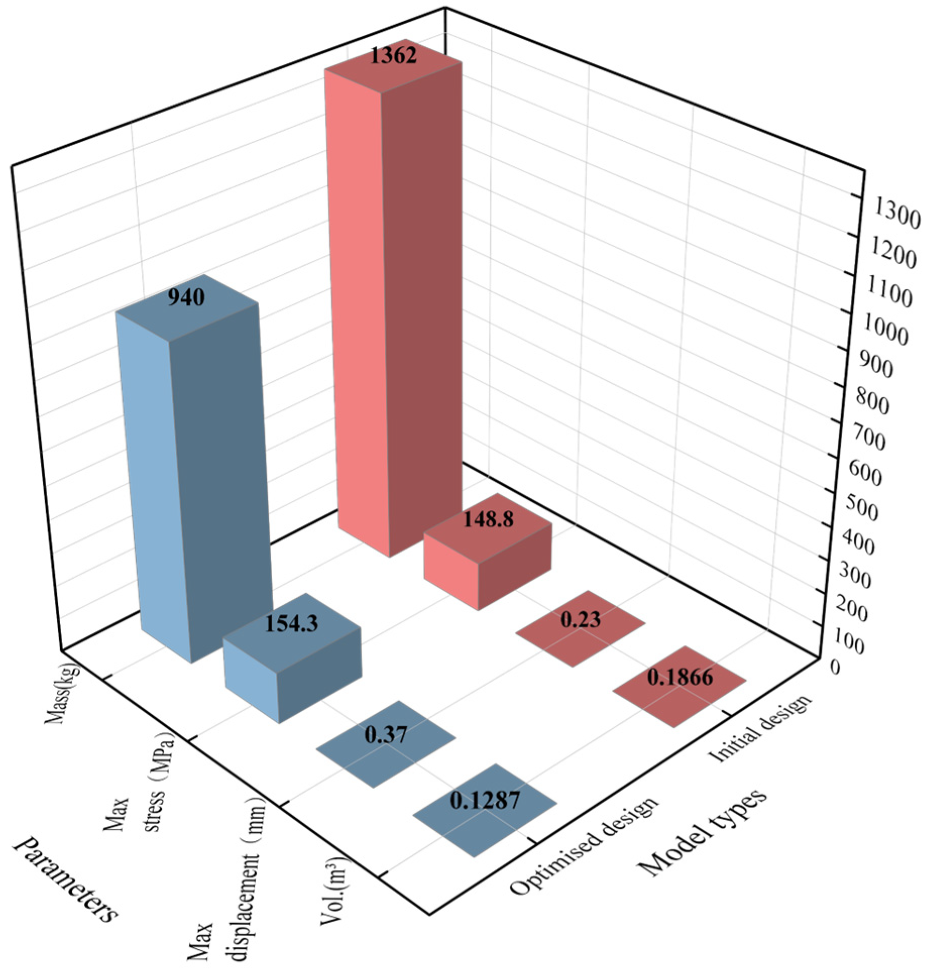
- Enhanced compatibility with engineering constraints, including non-design domain binding and multi-loadcase coupling. Applied to the lightweight design of a hydraulic torque converter adapter bracket, the framework achieved 31% volume reduction while meeting strength/stiffness requirements, demonstrating engineering viability.
2. Materials and Methods
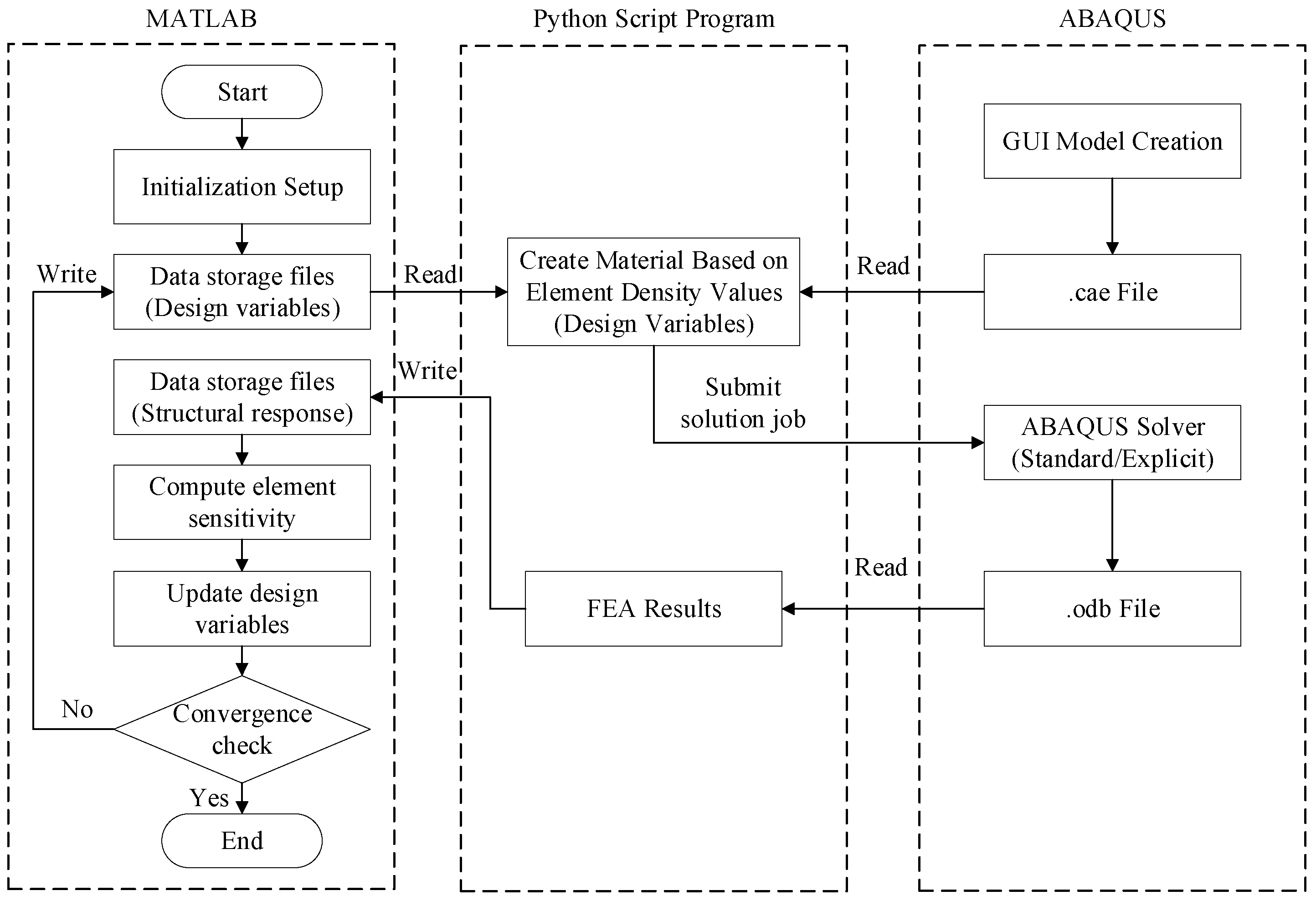
3. Architecture Design and Implementation Workflow of the ABAQUS–MATLAB Cooperative Framework
3.1. Hierarchical Architecture Design of the Cooperative Framework
3.2. MATLAB Master Control Program Design
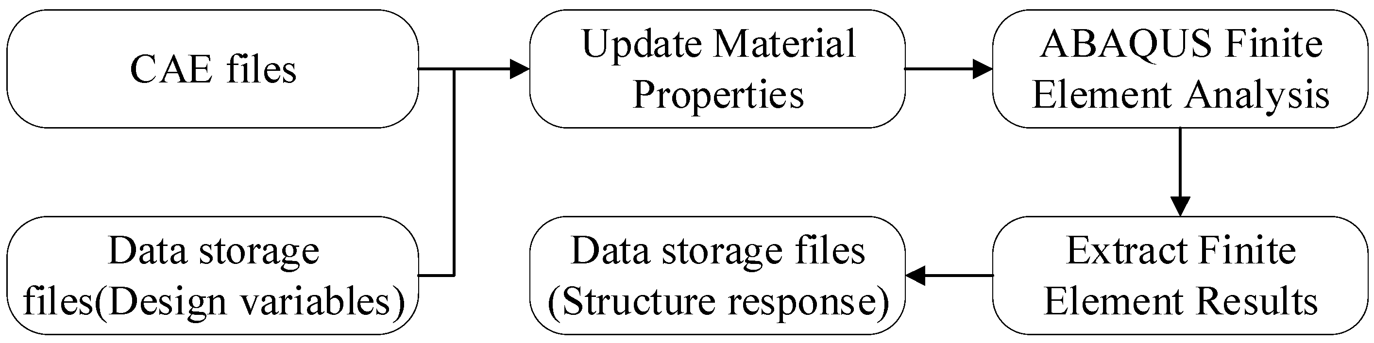
3.3. Python Scripting Implementation
4. Verification Examples
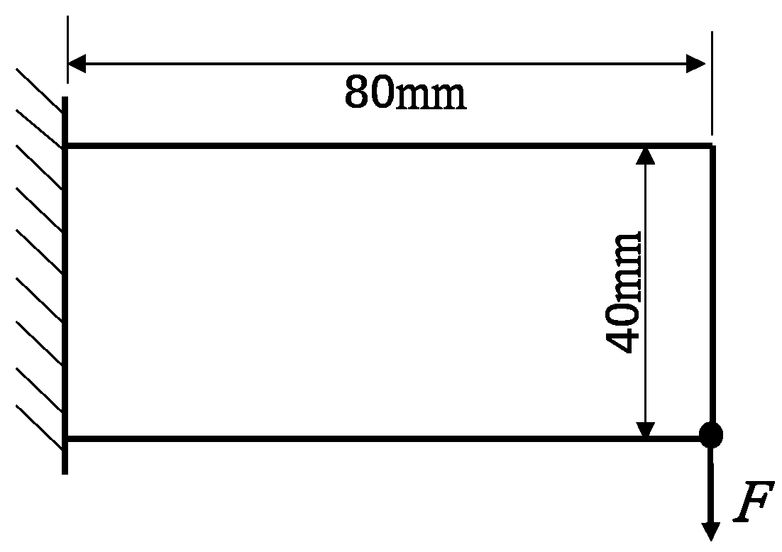
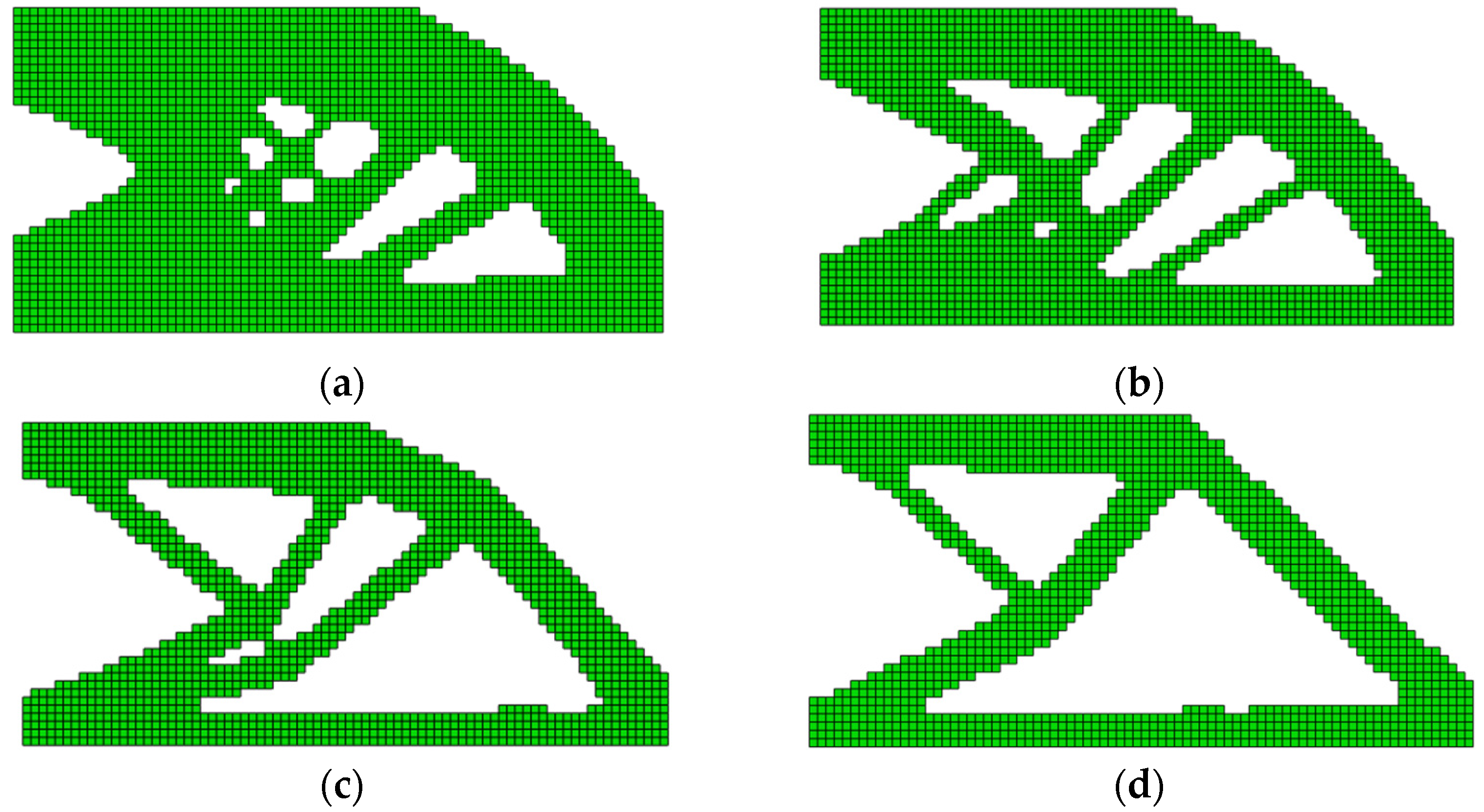
4.1. Topology Optimization of a 2D Cantilever Beam
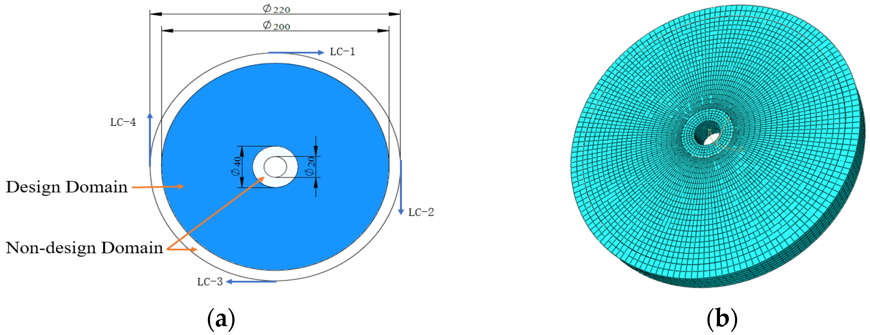
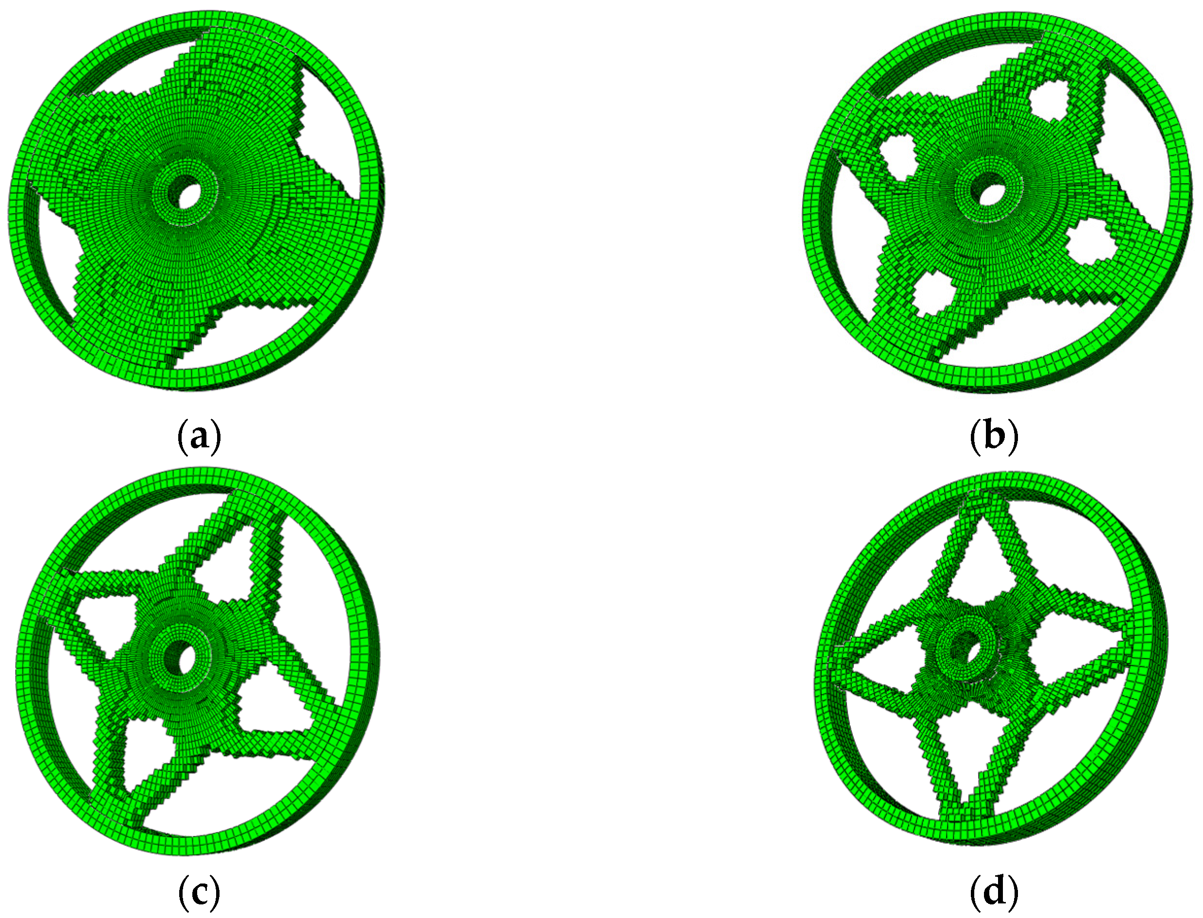
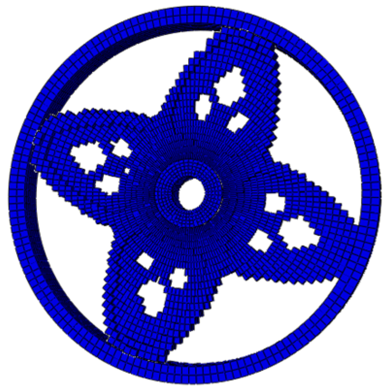
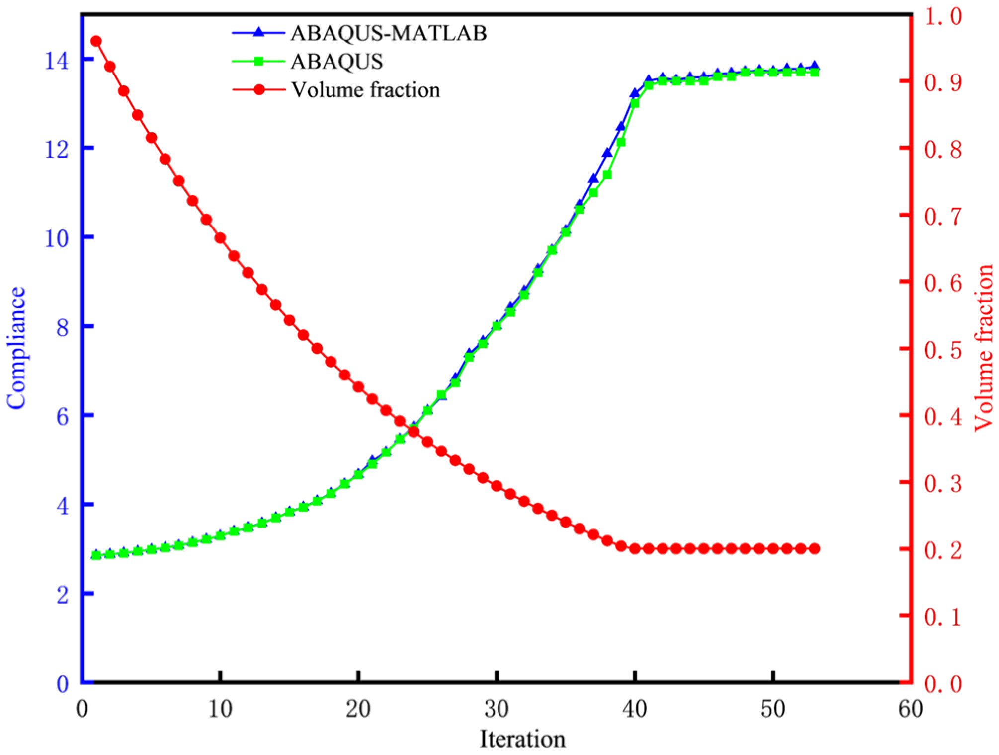
4.2. Lightweight Design of a 3D Wheel Hub
4.3. Comparative Analysis of 2D Beam and 3D Wheel Hub Optimization
- (1)
- An increase in element count: A multiplicative increase in the number of elements substantially prolongs finite element computation time in ABAQUS, while cross-platform data exchange time also rises proportionally.
- (2)
- Geometric complexity: The hub’s radial symmetry and fillets necessitated finer meshing to resolve stress gradients, whereas the beam’s rectilinear geometry allowed for uniform coarser meshes.
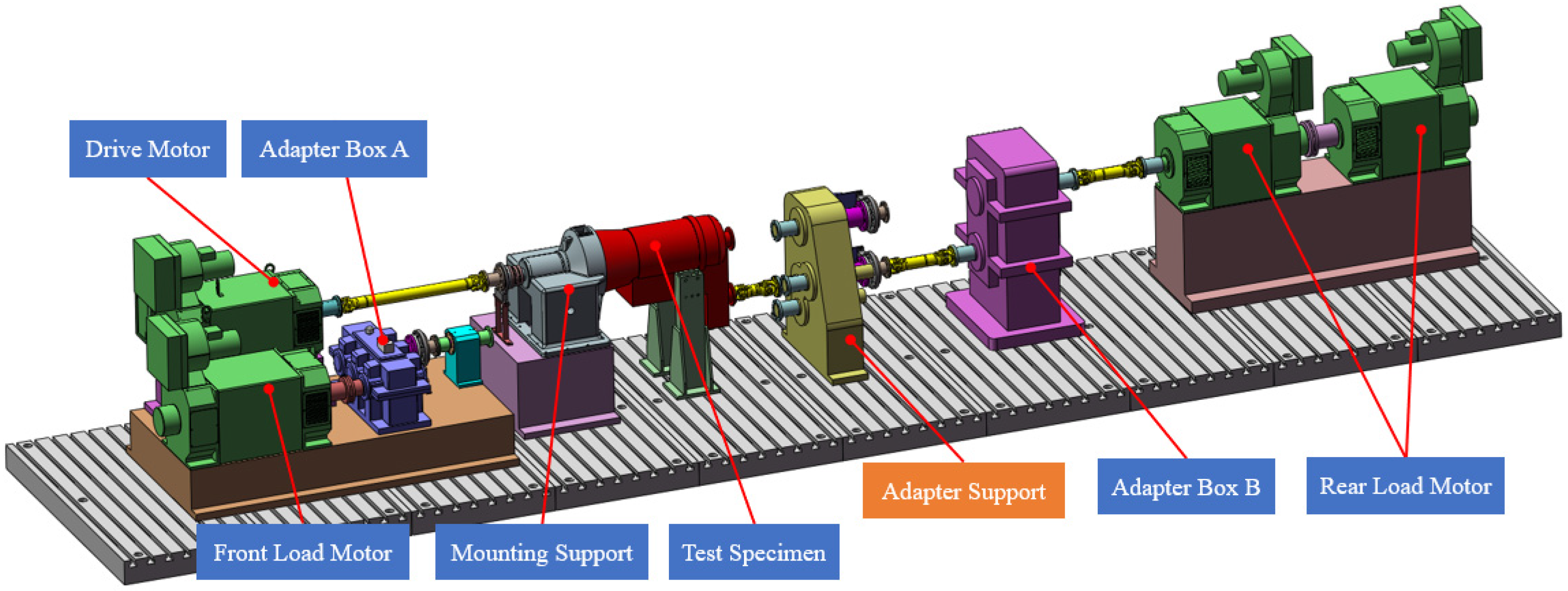
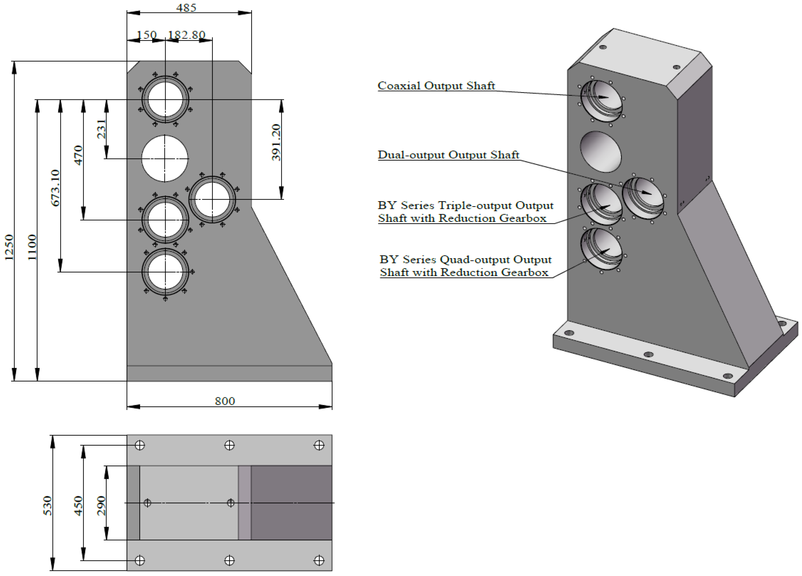
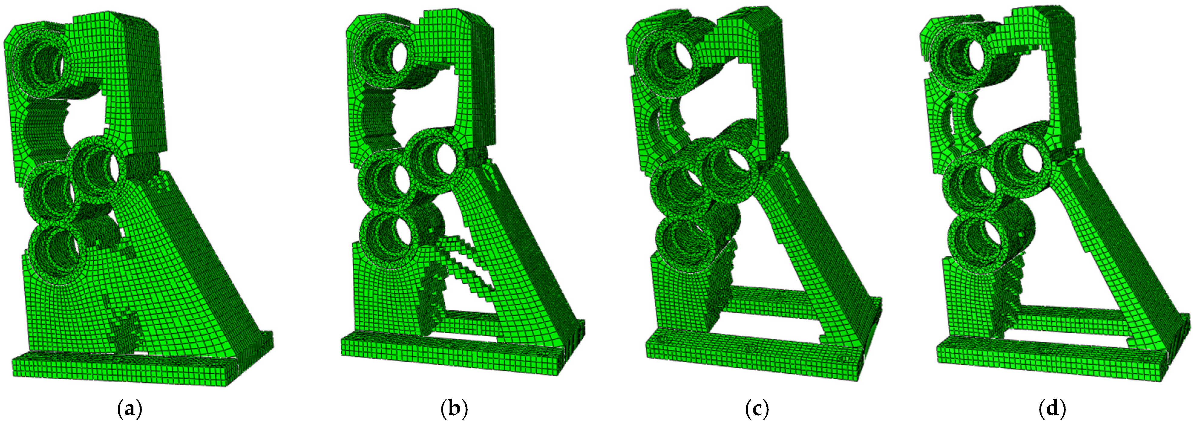
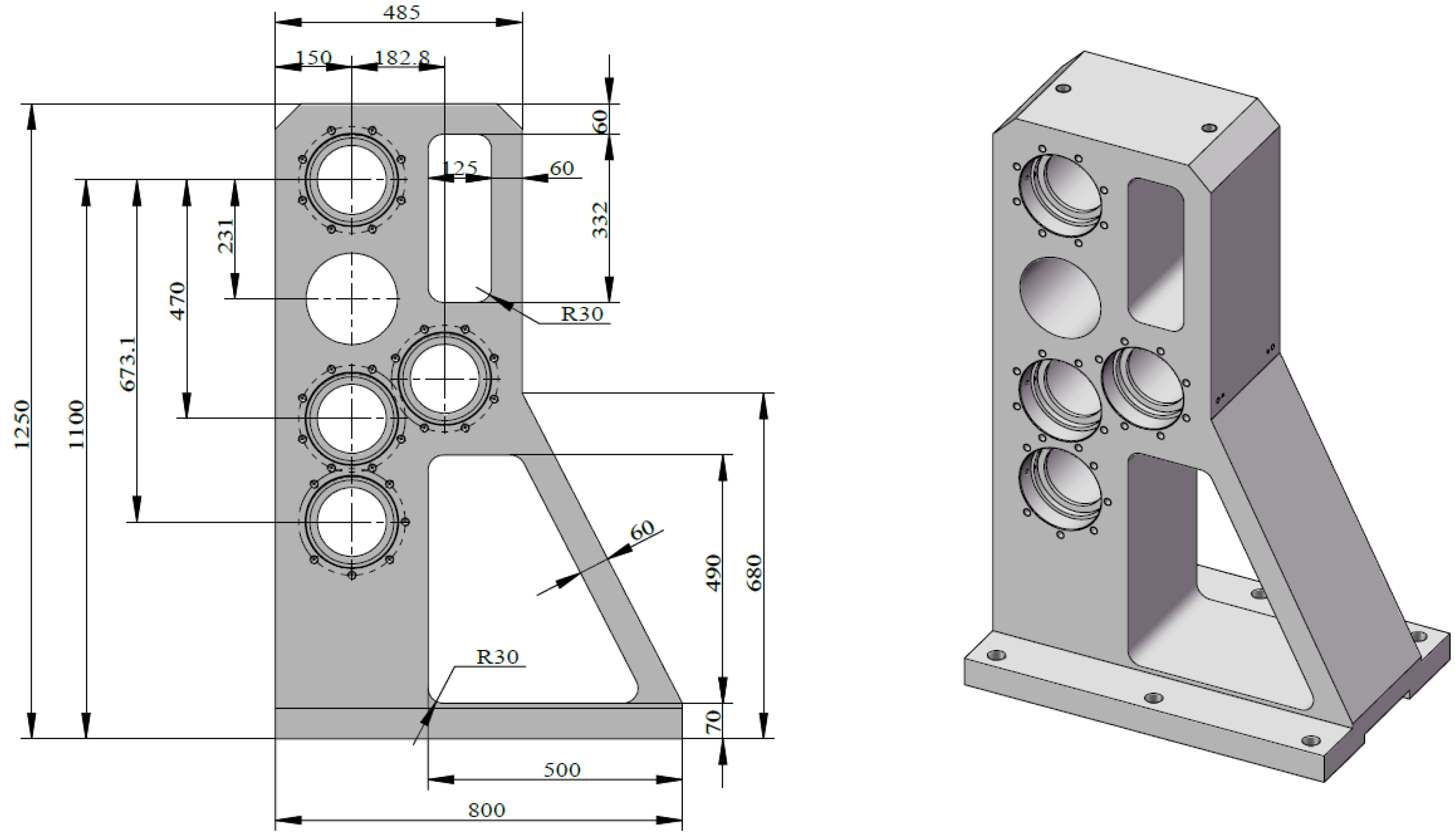
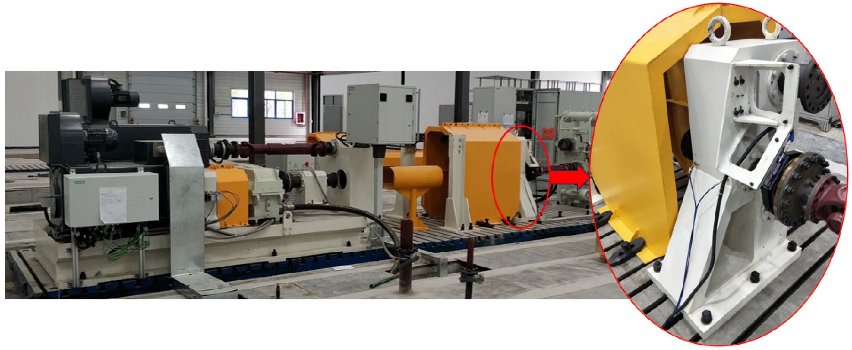
5. A Topology Optimization Engineering Application for a Hydraulic Transmission Test Bench Adapter Support
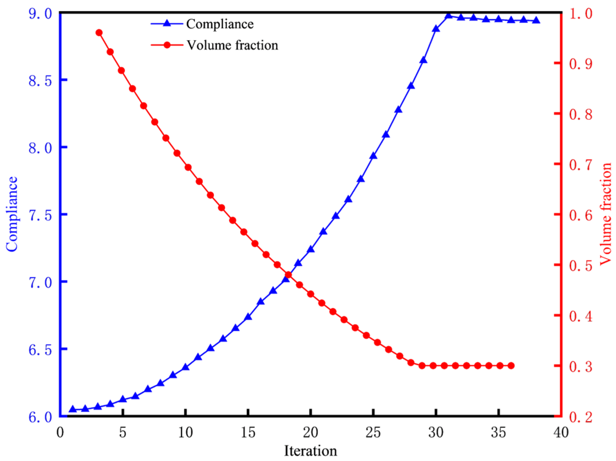
5.1. Optimization Design Implementation
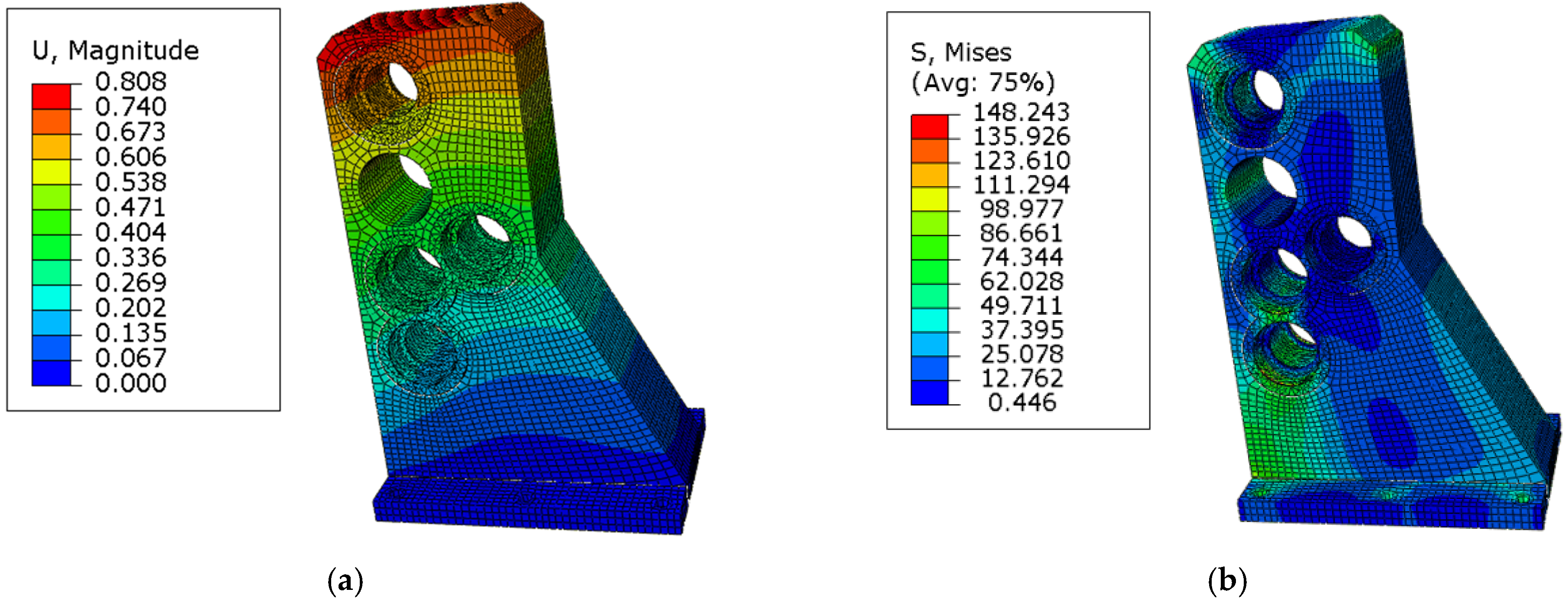
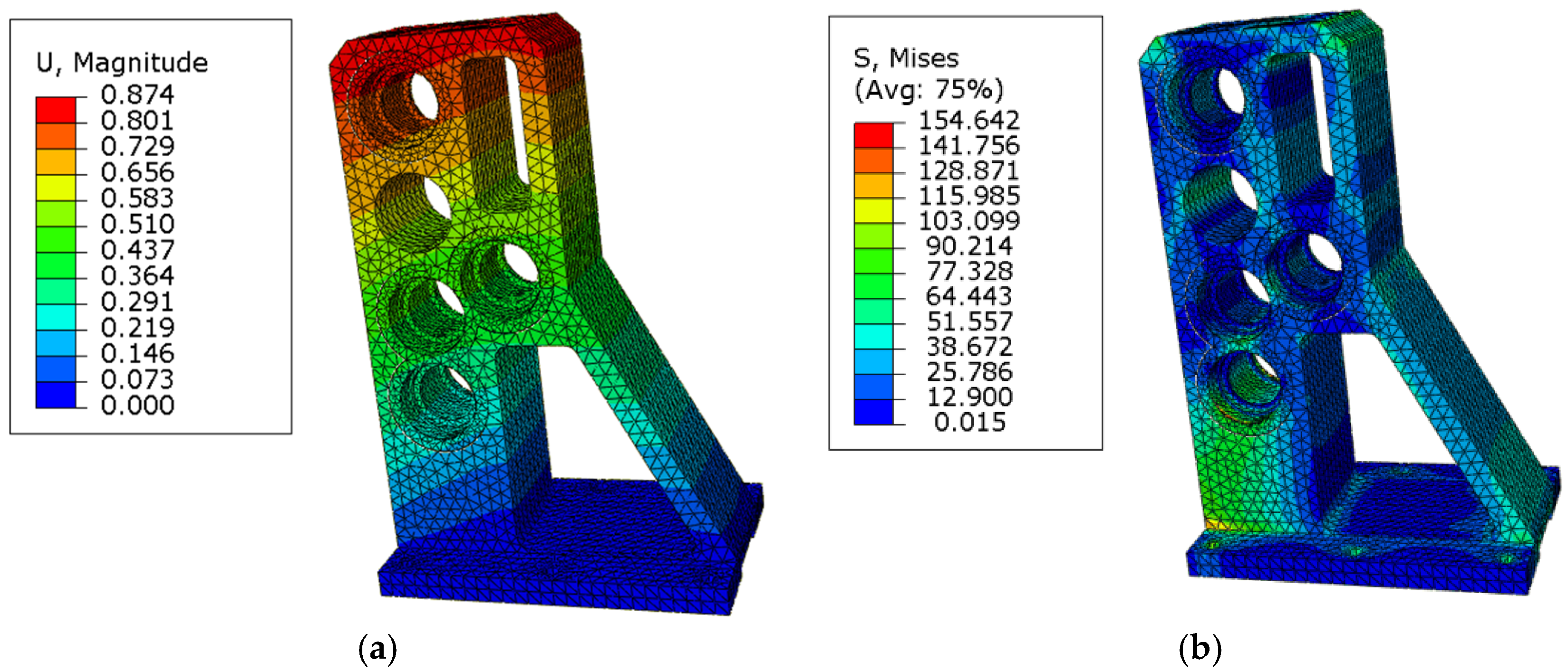
5.2. Engineering Validation and Application Value
6. Conclusions
Author Contributions
Funding
Institutional Review Board Statement
Informed Consent Statement
Data Availability Statement
Conflicts of Interest
References
- Bendsoe, M.P.; Kikuchi, N. Generating Optimal Topologies in Structural Design Using a Homogenization Method. Comput. Methods Appl. Mech. Eng. 1988, 71, 197–224. [Google Scholar] [CrossRef]
- Hurtado-Pérez, A.B.; Pablo-Sotelo, A.d.J.; Ramírez-López, F.; Hernández-Gómez, J.J.; Mata-Rivera, M.F. On Topology Optimisation Methods and Additive Manufacture for Satellite Structures: A Review. Aerospace 2023, 10, 1025. [Google Scholar] [CrossRef]
- Kim, B.-S.; Han, H.-W.; Chung, W.-J.; Park, Y.-J. Optimization of Gearbox Housing Shape for Agricultural UTV Using Structural-Acoustic Coupled Analysis. Sci. Rep. 2024, 14, 4145. [Google Scholar] [CrossRef]
- Elelwi, M.; Botez, R.M.; Dao, T.-M. Structural Sizing and Topology Optimization Based on Weight Minimization of a Variable Tapered Span-Morphing Wing for Aerodynamic Performance Improvements. Biomimetics 2021, 6, 55. [Google Scholar] [CrossRef]
- Srivastava, S.; Salunkhe, S.; Pande, S. Topology Optimization of Engine Bracket Arm Using BESO. Int. J. Simul. Multidisci. Des. Optim. 2023, 14, 2. [Google Scholar] [CrossRef]
- Gao, J.; Xiao, M.; Zhang, Y.; Gao, L. A Comprehensive Review of Isogeometric Topology Optimization: Methods, Applications and Prospects. Chin. J. Mech. Eng. 2020, 33, 87. [Google Scholar] [CrossRef]
- Wei, P.; Wang, W.; Yang, Y.; Wang, M.Y. Level Set Band Method: A Combination of Density-Based and Level Set Methods for the Topology Optimization of Continuums. Front. Mech. Eng. 2020, 15, 390–405. [Google Scholar] [CrossRef]
- Li, Z.; Xu, H.; Zhang, S. Moving Morphable Component (MMC) Topology Optimization with Different Void Structure Scaling Factors. PLoS ONE 2024, 19, e0296337. [Google Scholar] [CrossRef]
- Li, Z.; Xu, H.; Zhang, S. A Comprehensive Review of Explicit Topology Optimization Based on Moving Morphable Components (MMC) Method. Arch. Comput. Method Eng. 2024, 31, 2507–2536. [Google Scholar] [CrossRef]
- Yang, X.Y.; Xie, Y.M.; Steven, G.P.; Querin, O.M. Bidirectional Evolutionary Method for Stiffness Optimization. AIAA J. 1999, 37, 1483–1488. [Google Scholar] [CrossRef]
- Xia, L.; Xia, Q.; Huang, X.; Xie, Y.M. Bi-Directional Evolutionary Structural Optimization on Advanced Structures and Materials: A Comprehensive Review. Arch. Comput. Method Eng. 2018, 25, 437–478. [Google Scholar] [CrossRef]
- Huang, X.; Xie, Y.-M. A Further Review of ESO Type Methods for Topology Optimization. Struct. Multidiscip. Optim. 2010, 41, 671–683. [Google Scholar] [CrossRef]
- Ye, Z.; Pan, W. Discrete Variable Topology Optimization Using Multi-Cut Formulation and Adaptive Trust Regions. Struct. Multidiscip. Optim. 2025, 68, 25. [Google Scholar] [CrossRef]
- Liu, C.-H.; Huang, G.-F.; Chiu, C.-H. An Evolutionary Topology Optimization Method for Design of Compliant Mechanisms with Two-Dimensional Loading. In Proceedings of the 2015 IEEE International Conference on Advanced Intelligent Mechatronics (AIM), Busan, Republic of Korea, 7–11 July 2015; pp. 1340–1345. [Google Scholar]
- Alfouneh, M.; Tong, L. Topology Optimization of Nonlinear Structures with Damping under Arbitrary Dynamic Loading. Struct. Multidiscip. Optim. 2018, 57, 759–774. [Google Scholar] [CrossRef]
- Rostami, S.A.L.; Ghoddosian, A.; Kolahdooz, A.; Zhang, J. Topology Optimization of Continuum Structures under Geometric Uncertainty Using a New Extended Finite Element Method. Eng. Optim. 2022, 54, 1692–1708. [Google Scholar] [CrossRef]
- Latifi Rostami, S.A.; Kolahdooz, A.; Chung, H.; Shi, M.; Zhang, J. Robust Topology Optimization of Continuum Structures with Smooth Boundaries Using Moving Morphable Components. Struct. Multidiscip. Optim. 2023, 66, 121. [Google Scholar] [CrossRef]
- Bai, S.; Kang, Z. Robust Topology Optimization for Structures under Bounded Random Loads and Material Uncertainties. Comput. Struct. 2021, 252, 106569. [Google Scholar] [CrossRef]
- Habashneh, M.; Cucuzza, R.; Aela, P.; Movahedi Rad, M. Reliability-Based Topology Optimization of Imperfect Structures Considering Uncertainty of Load Position. Structures 2024, 69, 107533. [Google Scholar] [CrossRef]
- Mukherjee, S.; Lu, D.; Raghavan, B.; Breitkopf, P.; Dutta, S.; Xiao, M.; Zhang, W. Accelerating Large-Scale Topology Optimization: State-of-the-Art and Challenges. Arch. Computat. Methods Eng. 2021, 28, 4549–4571. [Google Scholar] [CrossRef]
- Zuo, Z.H.; Xie, Y.M. A Simple and Compact Python Code for Complex 3D Topology Optimization. Adv. Eng. Softw. 2015, 85, 1–11. [Google Scholar] [CrossRef]
- Deng, H.; Vulimiri, P.S.; To, A.C. An Efficient 146-Line 3D Sensitivity Analysis Code of Stress-Based Topology Optimization Written in MATLAB. Optim. Eng. 2022, 23, 1733–1757. [Google Scholar] [CrossRef]
- Kazakis, G.; Lagaros, N.D. Multi-Scale Concurrent Topology Optimization Based on BESO, Implemented in MATLAB. Appl. Sci. 2023, 13, 10545. [Google Scholar] [CrossRef]
- Smith, H.; Norato, J.A. A MATLAB Code for Topology Optimization Using the Geometry Projection Method. Struct. Multidiscip. Optim. 2020, 62, 1579–1594. [Google Scholar] [CrossRef]
- Chandrasekhar, A.; Suresh, K. TOuNN: Topology Optimization Using Neural Networks. Struct. Multidiscip. Optim. 2021, 63, 1135–1149. [Google Scholar] [CrossRef]
- Schiffer, G.; Ha, D.Q.; Carstensen, J.V. HiTop 2.0: Combining Topology Optimisation with Multiple Feature Size Controls and Human Preferences. Virtual Phys. Prototyp. 2023, 18, e2268603. [Google Scholar] [CrossRef]
- Kazakis, G.; Lagaros, N.D. Topology Optimization Based Material Design for 3D Domains Using MATLAB. Appl. Sci. 2022, 12, 10902. [Google Scholar] [CrossRef]
- Zhu, B.; Zhang, X.; Zhang, H.; Liang, J.; Zang, H.; Li, H.; Wang, R. Design of Compliant Mechanisms Using Continuum Topology Optimization: A Review. Mech. Mach. Theory 2020, 143, 103622. [Google Scholar] [CrossRef]
- Chen, Q.; Zhang, X.; Zhu, B. A 213-Line Topology Optimization Code for Geometrically Nonlinear Structures. Struct. Multidiscip. Optim. 2019, 59, 1863–1879. [Google Scholar] [CrossRef]
- Papazafeiropoulos, G.; Muniz-Calvente, M.; Martinez-Paneda, E. Abaqus2Matlab: A Suitable Tool for Finite Element Post-Processing. Adv. Eng. Softw. 2017, 105, 9–16. [Google Scholar] [CrossRef]
- Chen, L.; Zhang, H.; Wang, W.; Zhang, Q. Topology Optimization Based on SA-BESO. Appl. Sci. 2023, 13, 4566. [Google Scholar] [CrossRef]
- Sun, H.; Ma, L. Structural Topology Optimization by Combining BESO with Reinforcement Learning. J. Harbin Inst. Technol. (New Ser.) 2021, 28, 85–96. [Google Scholar]
- Teimouri, M.; Asgari, M. Developing an Efficient Coupled Function-Based Topology Optimization Code for Designing Lightweight Compliant Structures Using the BESO Algorithm. Optim. Eng. 2024, 25, 575–603. Available online: https://link.springer.com/article/10.1007/s11081-023-09808-w (accessed on 11 March 2025). [CrossRef]
- Lin, H.; Xu, A.; Misra, A.; Zhao, R. An ANSYS APDL Code for Topology Optimization of Structures with Multi-Constraints Using the BESO Method with Dynamic Evolution Rate (DER-BESO). Struct. Multidiscip. Optim. 2020, 62, 2229–2254. [Google Scholar] [CrossRef]
- Silva, C.J.G.; Lopes, R.F.F.; Domingues, T.M.R.M.; Parente, M.P.L.; Moreira, P.M.G.P. Crashworthiness Topology Optimisation of a Crash Box to Improve Passive Safety during a Frontal Impact. Struct. Multidiscip. Optim. 2025, 68, 3. [Google Scholar] [CrossRef]
- Huang, X.; Xie, Y.M. A New Look at ESO and BESO Optimization Methods. Struct. Multidiscip. Optim. 2008, 35, 89–92. [Google Scholar] [CrossRef]
- Han, Y. Stress-based bi-directional evolutionary topology optimization for structures with multiple materials. Eng. Comput. 2024, 40, 2905–2923. [Google Scholar] [CrossRef]
- Xiong, Y.; Lu, H.; Yan, X.; He, Y.; Xie, Y.M. Achieving Diverse Morphologies Using Three-Field BESO with Variable-Radius Filter. Eng. Struct. 2025, 322, 119049. [Google Scholar] [CrossRef]
- Tian, X.; Wang, Z.; Liu, D.; Liu, G.; Deng, W.; Xie, Y.; Wang, H. Jack-up Platform Leg Optimization by Topology Optimization Algorithm-BESO. Ocean Eng. 2022, 257, 111633. [Google Scholar] [CrossRef]
- Garcez, G.L.; Pavanello, R.; Picelli, R. Stress-Based Structural Topology Optimization for Design-Dependent Self-Weight Loads Problems Using the BESO Method. Eng. Optim. 2023, 55, 197–213. [Google Scholar] [CrossRef]
- ASME B30.7-2021; Winches (Safety Standard for Cableways, Cranes, Derricks, Hoists, Hooks, Jacks, and Slings). The American Society of Mechanical Engineers: New York, NY, USA, 2021.


| Mesh Type | Element Size (mm) | Number of Elements | Elastic Modulus (MPa) | Poisson’s Ratio | Evolutionary Rate | Penalization Factor | Filter Radius (mm) | Volume Fraction |
|---|---|---|---|---|---|---|---|---|
| CPS4 | 1 × 1 | 3200 | 1 | 0.3 | 2% | 3 | 3 | 40% |
| Number of Elements | MATLAB Platform | ABAQUS–MATLAB Framework |
|---|---|---|
| 3200 | 16 s | 812 s |
| 12,800 | 738 s | 1851 s |
| 51,200 | 6730 s | 3049 s |
| Mesh Type | Design Domain Element Size (mm) | Design Domain Element Count | Elastic Modulus (MPa) | Poisson’s Ratio | Evolutionary Rate | Penalization Factor | Filter Radius (mm) | Volume Fraction |
|---|---|---|---|---|---|---|---|---|
| C3D8 | 4 | 15,600 | 1 | 0.3 | 4% | 3 | 10 | 20% |
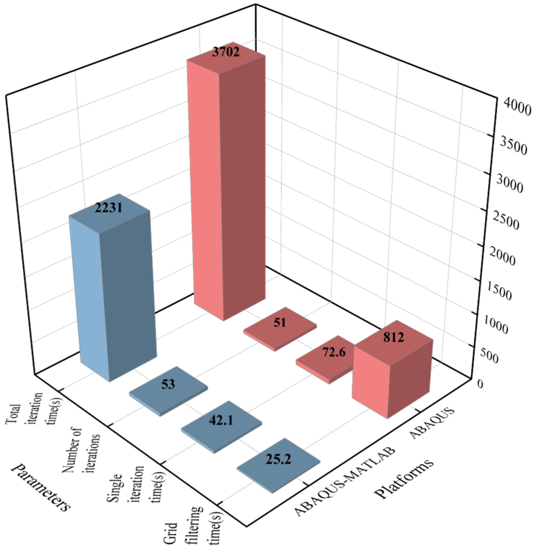
| Metric | ABAQUS Platform | ABAQUS–MATLAB Platform |
|---|---|---|
| Total iteration time (s) | 3702 | 2231 |
| Number of iterations | 51 | 53 |
| Single iteration time (s) | 72.6 | 42.1 |
| Grid filtering time (s) | 812 | 25.2 |
| Parameter | 2D Cantilever Beam | 3D Wheel Hub |
|---|---|---|
| Element count | 3200 | 15,600 |
| Iterations to convergence | 60 | 60 |
| Total computation time | 1124 s | 3049 s |
| Key geometric features | Rectilinear | Radial symmetry, fillets |
| Mesh Type | Design Domain Element Size (mm) | Design Domain Element Count | Elastic Modulus (MPa) | Poisson’s Ratio | Evolutionary Rate | Penalization Factor | Filter Radius (mm) | Volume Fraction |
|---|---|---|---|---|---|---|---|---|
| C3D8 | 18 | 24,016 | 130,000 | 0.25 | 4% | 3 | 50 | 30% |
| Parameters | Initial Design | Optimized Design |
|---|---|---|
| Volume (m3) | 0.1866 | 0.1287 |
| Mass (kg) | 1362 | 940 |
| Max. displacement (mm) | 0.808 | 0.874 |
| Max. stress (MPa) | 148.2 | 154.6 |
Disclaimer/Publisher’s Note: The statements, opinions and data contained in all publications are solely those of the individual author(s) and contributor(s) and not of MDPI and/or the editor(s). MDPI and/or the editor(s) disclaim responsibility for any injury to people or property resulting from any ideas, methods, instructions or products referred to in the content. |
© 2025 by the authors. Licensee MDPI, Basel, Switzerland. This article is an open access article distributed under the terms and conditions of the Creative Commons Attribution (CC BY) license (https://creativecommons.org/licenses/by/4.0/).
Share and Cite
Sun, D.; Yang, X.; Liu, H.; Yang, H. BESO Topology Optimization Driven by an ABAQUS-MATLAB Cooperative Framework with Engineering Applications. Appl. Sci. 2025, 15, 4924. https://doi.org/10.3390/app15094924
Sun D, Yang X, Liu H, Yang H. BESO Topology Optimization Driven by an ABAQUS-MATLAB Cooperative Framework with Engineering Applications. Applied Sciences. 2025; 15(9):4924. https://doi.org/10.3390/app15094924
Chicago/Turabian StyleSun, Dong, Xudong Yang, Hui Liu, and Hai Yang. 2025. "BESO Topology Optimization Driven by an ABAQUS-MATLAB Cooperative Framework with Engineering Applications" Applied Sciences 15, no. 9: 4924. https://doi.org/10.3390/app15094924
APA StyleSun, D., Yang, X., Liu, H., & Yang, H. (2025). BESO Topology Optimization Driven by an ABAQUS-MATLAB Cooperative Framework with Engineering Applications. Applied Sciences, 15(9), 4924. https://doi.org/10.3390/app15094924