Article

A Partitioned Rigid Element–Interface Element–Finite Element Method (PRE-IE-FE) for the Slope Stability Analysis of Soil–Rock Binary Structures

1
Powerchina Huadong Engineering Corporation Limited, Hangzhou 311122, China
2
Nanjing Hydraulic Research Institute, Nanjing 210029, China
3
College of Water Conservancy and Hydropower Engineering, Hohai University, Nanjing 210024, China
*
Author to whom correspondence should be addressed.
Appl. Sci. 2025, 15(9), 4903; https://doi.org/10.3390/app15094903
Submission received: 11 February 2025 / Revised: 16 April 2025 / Accepted: 24 April 2025 / Published: 28 April 2025
(This article belongs to the Special Issue Structural Health Monitoring for Concrete Dam)

Abstract

:
Soil–rock binary structure slopes are a unique and common phenomenon in water conservancy and geotechnical engineering, with complex stability issues that challenge traditional evaluation methods. This paper proposes the Partitioned Rigid Element–Interface Element–Finite Element (PRE-IE-FE) method, a novel numerical technique that addresses computational efficiency and accuracy in slope stability analysis. The method integrates composite destabilization modes along the soil interior, soil–rock contact surface, and rock structural surfaces, ensuring high computational performance. A slope instability criterion for PRE-IE-FE is established through derived control equations, a developed calculation program, and the strength reduction method. Case studies validate the method’s effectiveness and practicality, offering innovative solutions for similar engineering challenges.

1. Introduction

The soil–rock binary structural slope is a common yet specialized slope in hydraulic and geotechnical engineering [1,2,3]. These slopes typically have an upper part composed of stockpiled soil and a lower part made of weathered rock. They are widely distributed along transportation corridors and reservoirs in mountainous and river valley areas. In these slopes, the soil body is usually exposed at the surface, while the rock body lies underground. As a result, many studies treat them as stacked layer soil slopes using traditional homogeneous slope analysis methods, which do not consider their distinct dual structural features. Consequently, research on these slopes is relatively limited compared to studies on conventional earth and rocky slopes [4].
Engineering interventions such as road construction, channel excavation, dam building, or river training, along with natural geological events like earthquakes and extreme weather, such as heavy rainfall, may gradually expose the lower rock mass. When these slopes are disturbed by construction activities, heavy rainfall, fluctuations in groundwater levels, or reservoir changes, the soil–rock structure shows a different failure mode compared to homogeneous slopes. In this failure mode, sliding occurs simultaneously within the soil, along the soil–rock contact surface, and on the rock structure surface. This complex instability can lead to larger landslides, posing significant risks to construction operations and nearby residents [5].
Addressing the complex discontinuous and nonlinear behaviors exhibited during the instability and failure process of rocky slopes, Zhao and Li [6] proposed a hybrid finite element method that treats the contacting bodies’ nodal displacements as unknowns and uses the local nodal contact forces as iterative variables. Although this method better addresses nonlinear frictional contact problems, it remains a continuum medium numerical method and cannot simulate the complete disengagement of the rock body’s structural surface. To overcome this limitation, Li et al. [7] proposed the partitioned finite elements and interface elements (PFE-IE) hybrid solution, which combines the block element method [8,9] and the interface element method [10,11]. This solution divides large nonlinear regions into several local regions that can be solved independently, thereby reducing computational resource consumption through parallel solving. It is also compatible with the strength reduction method for calculating stability and safety coefficients of rocky slopes [12,13,14]. In the PFE-IE solution process, when a rocky slope with a potential sliding surface along a weak structural plane reaches its limit state, the elastic deformation of the rock mass becomes negligible compared to the deformation at the structural plane. Thus, treating the rock mass as rigid bodies simplifies the computational model and reduces numerical integration workloads, thereby enhancing solving efficiency. Building on this rationale, Sheng et al. [15] proposed the partitioned rigid element and interface element (PRE-IE) method based on PFE-IE. This method decomposes the system into multiple rigid bodies and discontinuous interfaces, using interface contact forces and rigid body centroid displacements as hybrid variables. By neglecting elastic deformations in high-stiffness continuous regions and concentrating nonlinear iterative computations on discontinuous interfaces, PRE-IE maintains computational accuracy while improving the efficiency of stability analysis for rocky slopes.
The instability modes of soil–rock binary structure slopes involve the coupled behavior of a continuum medium (soil body) and a discontinuous medium (structural planes in rock masses). However, in research on the stability analysis of slopes with a soil–rock dual structure, most scholars assume that the lower rock mass in soil–rock binary structure slopes is stable and consists of non-sliding bedrock. The analysis then focuses on the sliding within the upper soil mass and along the soil–rock interface using traditional limit equilibrium or finite element methods [16,17]. However, this approach neglects possible damage within the lower rock body and does not reflect the actual stability of the slope accurately [18]. The Finite Difference Method (FDM) is another technique in geotechnical engineering that approximates differential equations with finite differences, converting them into discrete algebraic systems. FLAC, which uses an explicit finite difference scheme, is effective for modeling nonlinear behavior and large deformation problems in geotechnical materials, and it has been widely applied in practical projects [19]. Some researchers have used FLAC to analyze the overall stability of soil–rock binary structure slopes. This approach considers multiple failure modes more accurately by including sliding within the soil, along the soil–rock contact surfaces, and within the rock body structure [2]. Despite this, using the safety coefficient from traditional slope stability analyses to assess the reliability of these slopes presents challenges in computational efficiency. FLAC has several drawbacks. First, it usually requires command flow for pre-processing, which means that complex models need to be created in external software (e.g., the pre-processing module of ANSYS (2025 R1)) and then imported into FLAC, significantly increasing analysis time. Second, its explicit difference algorithm, although suitable for dynamic problems and nonlinear static problems with large deformations [19], demands a smaller time step for slope stabilization problems that mostly involve linear and small deformations. This requirement increases computational time compared to the finite element method. Moreover, the convergence rate of the Finite Difference Method drops when the finite element size or the material’s elastic modulus is large. In post-processing, FLAC’s finite difference strength reduction technique, using the built-in SOLVE fos command, converges more slowly for complex slope models. Consequently, while FLAC excels in analyzing instability mechanisms and damage modes in soil–rock binary structure slopes, its lower efficiency in safety factor calculation limits its broader application in reliability analysis.
Developing a numerical simulation method that can accurately reproduce the complex instability patterns of soil–rock binary structure slopes and improving computational efficiency is therefore critical. The PRE-IE method efficiently simulates sliding along structural planes in rock masses by discretizing the rock into rigid elements and employing interface elements to handle contact nonlinearities [15]. However, it cannot describe the continuous elastic deformation of the soil body. Therefore, building on the PRE-IE method [15], this study proposes the Partitioned Rigid Element–Interface Element–Finite Element (PRE-IE-FE) method, which integrates the finite element method (FEM) to simulate the continuum medium behavior of the overlying soil body, while coupling with the PRE-IE method to rigorously capture the discontinuous and nonlinear interactions at soil–rock contact surfaces and structural planes within the rock mass. This combined approach enables full-process modeling of composite failure modes in soil–rock binary structure slopes. We also combine the PRE-IE-FE method with the strength reduction method to create a slope instability criterion that better ensures the stability of soil–rock binary structure slopes. The effectiveness of this new method is verified through several examples [12,13,14,15].

2. Common Destabilization Modes of Slopes with Soil–Rock Dichotomies

The types of soil–rock binary structure slopes are complex and diverse. Sun [2] compiled a substantial corpus of pertinent information and proposed a classification system based on criteria such as the morphology of the soil–rock contact surface, the properties of the soil–rock contact surface, the tendency of the top face of the slope, the thickness of the overlying soil layer, and the number of excavation steps in the overburden. The soil–rock binary structure slopes are categorized into the various types shown in Table 1.
However, it should be noted that some of these slope types are rare, and certain types of slopes (e.g., slopes with anti-dip yielding soil–rock contact surfaces and slopes with thin overlying soil layers) are not susceptible to slope instability. In light of the findings of Tang et al. [5], the two most prevalent soil–rock binary structural slope types that are prone to destabilization, along with their associated destabilization modes and sliding surface patterns, are presented in Table 2.
The first kind of soil–rock binary structure slope is characterized by a loose soil body piled up at the upper part and stable bedrock at the lower part. The strength parameters of the loose soil body and the soil–rock contact surface are significantly less than those of the bedrock, resulting in damage occurring primarily in the inner part of the loose soil body and at the soil–rock contact surface. The destabilization mode is primarily evidenced by rotational sliding within the loose-packed soil body and sliding of the packed soil body along the soil–rock contact surface. The sliding surface exhibits a composite morphology, comprising both a circular arc shape and a contact surface shape.
The second soil–rock binary structure of the upper part of the slope consists of an accumulation of soil or fully weathered rock. The lower part is a rock body with a weak structural surface, which is characterized by a lower strength parameter than that of the upper part of the soil body and the soil–rock contact surface. For example, the parallel lines in the picture of the second type of slope structure in Table 2 represent the weak structural surface. Consequently, damage occurs not only within the soil body and at the soil–rock contact surface but also on the weak structural surface. The instability mode is manifested in the rock body along the weak structural surface through linear sliding, which causes the upper part of the soil body to undergo rotational sliding and sliding along the soil–rock contact surface. The sliding surface takes the form of an arc, the contact surface has the shape of a composite sliding surface, and the folding line is composed of the aforementioned sliding surfaces.
In light of the two typical instability modes of soil–rock binary structure slopes outlined in this section, it is evident that the numerical simulation method selected for the stability analysis of such slopes must possess the capacity to simulate the continuous medium behavior of the overlying soil. Additionally, it is imperative that the method accurately reflects the discontinuous and nonlinear behaviors of the soil–rock contact surfaces, as well as the rock structure surfaces. Accordingly, the following section will present a coupled numerical simulation method, the PRE-IE-FE method, which combines the finite element method and the PRE-IE method. This method will then be applied to the stability analysis of soil–rock binary structure slopes.

3. PRE-IE-FE

The finite element method (FEM), a continuum media method commonly employed in the numerical analysis of soil slopes, has been demonstrated to effectively describe the continuum damage behavior within the soil body [20,21,22,23,24]. In contrast, the PRE-IE method [15] has been demonstrated to be an effective approach for modeling the local discontinuities and contact nonlinear behavior of the rock mass when it is destabilized along the structural plane, while also offering high computational speed. Accordingly, as illustrated in Figure 1, the soil–rock binary structure slope, comprising the overlying soil body, the soil–rock contact surface between the soil body and the rock body, the lower rock body, and the weak structural surface in the rock body, can be regarded as a continuous medium that necessitates consideration of elastic deformation. Furthermore, a finite element mesh can be delineated on top of it. The finite elements in the upper part and the rigid elements in the lower part are coupled by interface elements on the soil–rock contact surface. Subsequently, the lower rock body and the internal weak structural surfaces can be structurally discretized and meshed in accordance with the previously described PRE-IE method. For detailed meshing procedures, refer to [15].

3.1. Core Equations of the PRE-IE Method

The PRE-IE method, proposed by Sheng et al. [15], simplifies rock masses into rigid bodies connected by interface elements. This approach avoids complex elastic deformation calculations and focuses on structural plane sliding. Its governing equations are derived from the principle of minimum potential energy, with rigid body motion and interface contact forces as key variables. Below are the core equations that support PRE-IE.

3.1.1. Equations of Rigid Element

Rigid elements assume no internal elastic deformation. The displacements, u , of all nodes within a rigid element are determined by its centroid displacement and rotation, expressed as follows:
u = u x u y u z = W γ e
where W is the rigid displacement transformation matrix, and γ e is the displacement of the rigid body centroid. This formulation ensures displacement consistency across nodes under external forces and significantly simplifies numerical calculations.

3.1.2. Equations of Interface Element

Interface elements model contact surfaces or structural planes between rigid elements using a thin-layer finite element formulation. The displacements of the upper and lower surfaces are interpolated as follows:
u u p = N 1 u 1 + N 2 u 2 + N 3 u 3 + N 4 u 4 = N a u p e
u d o w n = N 1 u 5 + N 2 u 6 + N 3 u 7 + N 4 u 8 = N a d o w n e
where N is the shape function matrix of the four-node quadrilateral isoparametric element u is the nodal displacement, a u p e is the nodal displacement array on the upper surface of the interface element, and a d o w n e is the nodal displacement array on the lower surface of the interface element.
The displacement difference, Δ u , between upper and lower surfaces of an interface element is described as follows:
Δ u = Δ u x Δ u y Δ u z = u u p u d o w n = B a e
where u u p is the displacement of any point on the upper surface of the interface element, and u d o w n is the nodal displacement. B is the shape function matrix, and a e is the nodal displacement array.
The displacement difference, Δ u , between the two surfaces is used to compute local strain, ε , as follows:
ε = γ z x γ z y ε z = Δ u x t Δ u y t Δ u z t = Δ u t
Combined with the elastic matrix, D , the interface stress, σ , is derived as follows:
σ = τ z x τ z y σ z = t k x x 0 0 0 t k y y 0 0 0 t k z z γ z x γ z y ε z = D ε
where D is the elastic matrix of the structural plane, k z z is the normal stiffness, k x x and k y y are the tangential stiffnesses, t is the element thickness, γ z x and γ z y are tangential strains, and ε z is normal strain.

3.1.3. Equations of PRE-IE

To ensure consistency in displacement and contact force between rigid elements and interface elements, Lagrange multipliers are introduced to couple them. The energy functional is defined as follows:
Π = Π f + Π i + Π c
where Π f is the potential energy of rigid elements, Π i is the potential energy of interface elements, and Π c represents the constraint terms enforcing compatibility conditions at interfaces. The detailed formulation is provided in Equation (19) of reference [15].
By setting the first variation of Π to zero, the mixed-variable governing equations are obtained as follows:
K γ γ K γ f K f γ K f f γ f = 0 P
where K f γ couples contact forces, f , and rigid displacements, γ , and P represents external loads. The specific forms of K γ γ , K γ f , K f γ , and K f f are described in the literature [15].
Meanwhile, the PRE-IE method incorporates a nonlinear contact iterative strategy that updates the contact node pairs based on contact states (stick, slip, debonding) to ensure computational consistency with physical reality. For a detailed implementation of this strategy, refer to [15].
The aforementioned processes constitute the fundamental theoretical framework of the PRE-IE method, serving as the theoretical foundation for the subsequent development of the PRE-IE-FE method.

3.2. The Governing Equations for PRE-IE-FE

Prior to deriving the governing equations of PRE-IE-FE, it is first necessary to construct the coupled interface elements between the finite element and rigid body elements. Although interface elements are present in both the PRE-IE and PRE-IE-FE methods, the interface elements between finite elements and rigid body elements in the PRE-IE-FE method, as presented in this paper, differ from those between rigid body elements in the PRE-IE method due to the disparate forms of displacement exhibited by finite elements and rigid body elements. In particular, the displacements of any given point on the upper and lower surfaces of the aforementioned interface element are obtained through interpolation, utilizing the displacements of the form center points of the upper and lower rigid body elements. In contrast, the displacement of any point on the upper surface of the interface element between a finite element and a rigid element is obtained by interpolating the displacements of the finite element nodes. The displacement of any point on the lower surface is obtained by interpolating the displacement of the shape center point of the rigid element.
In this paper, the two-dimensional four-node quadrilateral thin-layer finite element shown in Figure 2 will be employed as the interface element, and the governing equations of PRE-IE-FE will be derived on the basis of this finite element.

3.2.1. Governing Equations of Thin-Layer Interface Elements

The length of the thin-layer finite element is l , the thickness is t , and the width perpendicular to the direction of the x y plane is w . A local coordinate system, s ,   n , is established on the thin-layer finite element, with s as the tangential direction of the interface and n as the normal direction of the interface. Assuming that the finite element on the upper part of the interface element is a linear element, the tangential displacement, u u p , and normal displacement, v u p , at any point on the upper surface of the thin-layer finite element can be obtained via the linear interpolation of the displacements of nodes 1 and 2 belonging to the finite element, as follows:
u n p = 1 2 1 2 s l u 1 + 1 2 1 + 2 s l u 2
v u p = 1 2 1 2 s l v 1 + 1 2 1 + 2 s l v 2
where u 1 and v 1 are the tangential and normal displacements of finite element node 1, respectively, and u 2 and v 2 are the tangential and normal displacements of finite element node 2, respectively.
Since the lower part of the interface element is a rigid body element, the normal displacement, u d o w n , and tangential displacement, v d o w n , at any point on the lower surface of the thin-layer finite element can be obtained by interpolating the displacement at the centroid point, c , of the rigid body element shape, as follows:
u d o w n = u c + n c t 2 θ c
v d o w n = v c + s s c θ c
where u c and v c are the tangential and normal of the rigid body element centroid, c , respectively, and θ c is the angular displacement (positive in the counterclockwise direction) of the rigid element rotating around the centroid. ( s c , n c ) is the coordinate of the rigid body element centroid, c , in the local coordinate system. s represents the tangential coordinate of any point on the lower part of the interface element, while n represents the normal coordinate of any point on the lower part of the interface element. Equations (11) and (12) are only suitable for small angular displacements.
Then, the tangential displacement difference, Δ u , and normal displacement difference, Δ v , between the upper and lower surfaces of the thin finite element can be expressed as follows:
Δ u = u u p u d o w n = 1 2 1 2 s l u 1 + 1 2 1 + 2 s l u 2 u c n c + t 2 θ c
Δ v = v u p v d o w n = 1 2 1 2 s l v 1 + 1 2 1 + 2 s l v 2 v c s s c θ c
Combining Equations (13) and (14) yields an expression in matrix form for the difference between the upper and lower surface displacements, U, of the thin finite element, as follows:
Δ u = Δ u Δ v = 1 2 1 2 s l u 1 + 1 2 1 + 2 s l u 2 u c n c + t 2 θ c 1 2 1 2 s l v 1 + 1 2 1 + 2 s l v 2 v c s s c θ c = 1 2 1 2 s l 0 1 2 1 + 2 s l 0 1 0 n c + t 2 0 1 2 1 2 s l 0 1 2 1 + 2 s l 0 1 ( s s c ) u 1 v 1 u 2 v 2 u c v c θ c = B a B γ a e γ e = B a a e + B γ γ e
where B a is the shape function matrix of the finite element, a e = u 1 v 1 u 2 v 2 T is the finite element node displacement array in the upper part of the thin finite element, B γ is the shape function matrix of the rigid element, and γ e = u c v c θ c T is the rigid element form center point displacement array in the lower part of the thin finite element.
Since the thickness of the thin-layer finite element is much smaller than its length, only the normal strain, ε n , in the normal direction, n , and the shear strain, γ s , along the tangential direction, s , are considered. Consequently, the thin-layer element exhibits normal stress, σ n , and shear stress, τ s .
Then, the strain, ε , and stress, σ , of the thin finite element can be expressed as follows:
ε = γ s ε n = 1 t Δ u = 1 t Δ u Δ v = 1 t B a a e + B γ γ e
σ = τ s σ n = t k s 0 0 t k n γ s ε n = D ε = 1 t D B a a e + B γ γ e
where D is the stiffness matrix of the thin-layer finite element, where k n is the normal stiffness coefficient and k s is the tangential stiffness coefficient.

3.2.2. Assembly of the Global Stiffness Matrix

Combining the equations above, the potential energy generalization of the thin finite element can be expressed as follows:
Π P e = 1 2 S ε T σ d S = 1 2 S ε T D ε d S = 1 2 S 1 t 2 B a a e + B γ γ e T D B a a e + B γ γ e d S = 1 2 S 1 t 2 a e T B a T D B a a e d S + S 1 t 2 a e T B a T D B γ γ e d S + 1 2 S 1 t 2 γ e T B γ T D B γ γ e d S = 1 2 a e T K a e a e + a e T K a γ e γ e + 1 2 γ e T K γ e γ e
where K a e , K a γ e , and K γ e are the finite element stiffness matrix, the finite element stiffener element coupling stiffness matrix, and the stiffener element stiffness matrix in the thin finite element, respectively, of the following form:
K a e = S 1 t 2 B a T D B a d S
K a γ e = S 1 t 2 B a T D B γ d S
K γ e = S 1 t 2 B γ T D B γ d S
Then, the total potential energy generalization, Π P , of the interface element between the finite element and the rigid body element in the system can be expressed as the sum of the potential energy generalizations of the individual thin-layer elements, as follows:
Π P = e Π P e = 1 2 a T e ( G a T K a e G a ) a + a T e ( G a T K a γ e G γ ) γ + 1 2 γ T e ( G γ T K γ e G γ ) γ
where G a is the transformation matrix of the finite element nodal displacement array, a , of the system and the finite element nodal displacement array, a e , of the finite element, i.e., a e = G a a , and G y is the transformation matrix of the rigid body form-centered displacement array, γ , of the system and the rigid body form-centered displacement array, γ e , of the finite element, i.e., γ e = G γ γ .
Since the total potential energy of the system satisfies the principle of minimum potential energy, it is necessary to determine the stationary value of the total potential energy functional. According to the variational principle, the condition for the functional to attain a stationary value is that its first variation vanishes. This requires solving the following two equations:
Π P a = 0
Π P γ = 0
Upon substituting Equation (22) into both Equations (23) and (24) and subsequently solving the resulting equations, the following result is obtained:
e ( G a T K a e G a ) a + e ( G a T K a γ e G γ ) γ = 0
e ( G a T K a γ e G γ ) a + e ( G γ T K γ e G γ ) γ = 0
Let K a = e ( G a T K a e G a + G a T K a γ e G γ ) and K γ = e ( G a T K a γ e G γ + G γ T K γ e G γ ) be collapsed to obtain the governing equations for the thin finite element as follows:
K a a + K γ γ = 0

3.2.3. Coupled PRE-IE-FE Governing Equations

By combining the governing equations of finite elements with the governing equations of PRE-IE, the governing equations of PRE-IE-FE can be obtained as follows:
K F 0 0 K a K γ 0 0 K γ γ K γ f 0 K f γ K f f a γ f = P F 0 0 P
where K F is the stiffness matrix of the finite element and P F is the node load matrix of the finite element. Since the displacement of the upper surface of the interface element coupled with the finite element is linearly interpolated by the displacements of the finite element nodes, the finite elements in the finite element part need to be linear finite elements, such as three-node triangular finite elements or four-node quadrilateral finite elements. The expressions for the stiffness matrices and nodal load arrays of these finite elements can be found in related books on the finite element method [25], so this paper will not repeat this information. K γ γ , K γ f , K f γ , and K f f are the stiffness matrices of the PRE-IE, and P is the external loads of the PRE-IE. The detailed formulation is provided in Equations (24)–(28) of reference [15]. Since the control equations of the PRE-IE are derived for the three-dimensional case, the integration domain needs to be changed from the three-dimensional volume domain, V , into the two-dimensional area domain, S , and the corresponding form function matrix, elasticity matrix, transformation matrix, displacement column matrix, and contact force column matrix need to be changed into the two-dimensional form.
Since the PRE-IE-FE method employs the same nonlinear eigenstructure and contact algorithm as the PRE-IE method in reference [15], it is necessary to use the incremental iterative method to solve the governing equations shown in Equation (28) in order to compute the finite-element node displacements, a , rigid-body element center-of-form displacements, γ , and interfacial contact force, f .
The authors have completed the entire solution process by using the PRE-IE-FE computational program, which is described in detail in the following sections.

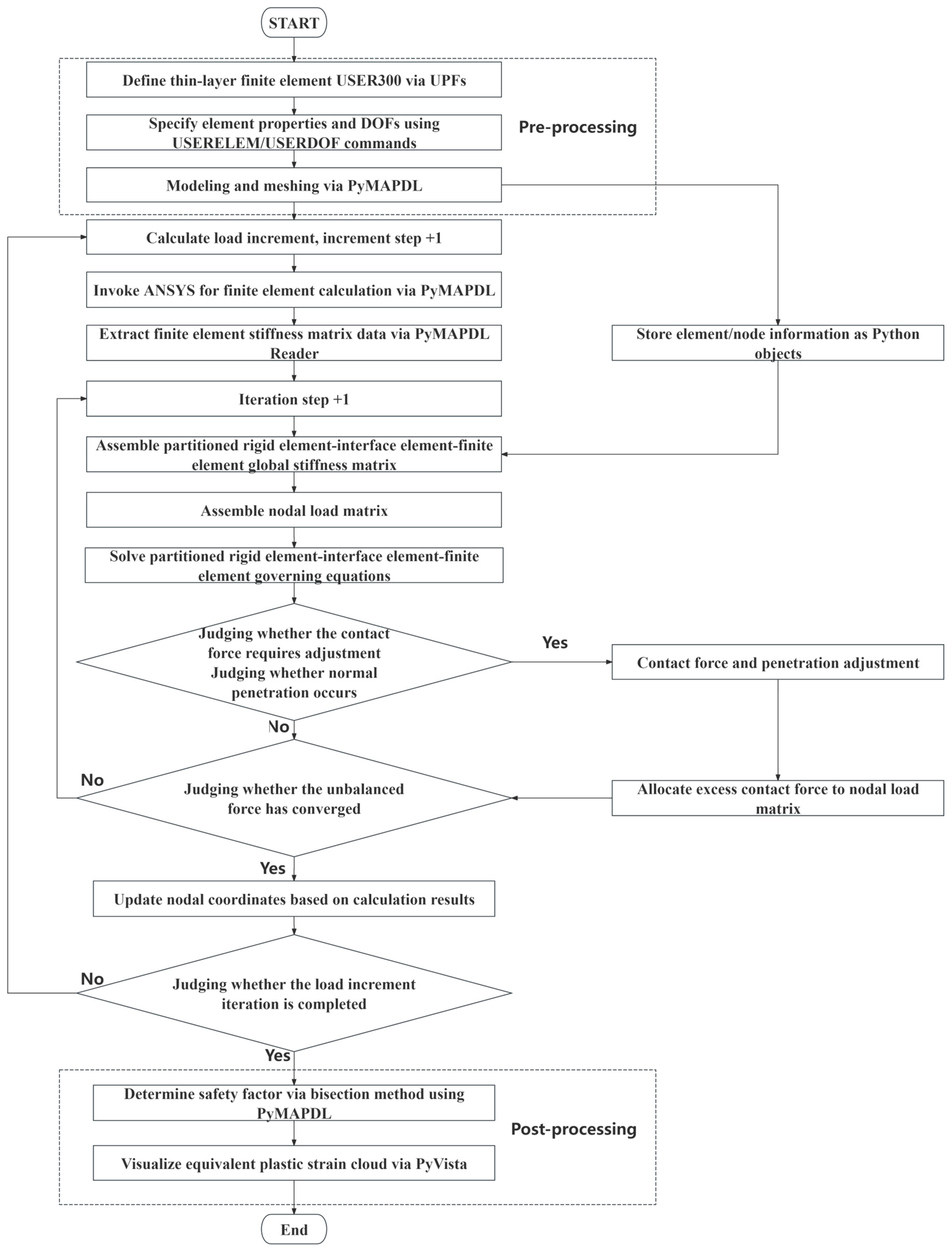
3.3. Calculation Process and Program Development for PRE-IE-FE

In reference [15], the authors developed the PRE-IE program using Python. However, the program is deficient in its pre-processing capabilities, necessitating the utilization of commercial pre-processing software for the construction and meshing of models. It is evident that the numerical integration speed of Python is slower than that of commercial software due to the inherent limitations of the programming language kernel and the absence of targeted optimization. Accordingly, in order to incorporate the superior pre-processing capabilities and computational solution performance of commercial software, the authors have completed the development of the PRE-IE-FE program, which is based on the PRE-IE program and includes the secondary development of commercial finite element software ANSYS.
Figure 3 illustrates the computational flow of the PRE-IE-FE program. The following sections describe the detailed steps of pre-processing, numerical computation, and post-processing in the program, based on this illustration.

3.3.1. Customized Units

The PRE-IE-FE method employs thin-layer finite elements as interface elements, a feature that is not present in the ANSYS finite element library. Consequently, in order to utilize ANSYS for modeling and meshing, it is necessary to customize thin-layer finite elements through the implementation of User Programmable Features (UPFs) within ANSYS [26].
The UserElem subroutine, which is used to create custom finite elements, contains a finite element named USER300 in the program file. In order to define a four-node quadrilateral with a thickness thin-layer finite element for 2D problems and an eight-node hexahedron with a thickness thin-layer finite element for 3D problems, it is necessary to first define the aforementioned finite elements. The aforementioned custom finite elements necessitate the alteration of the stiffness matrix variable eStiff and the external load array variable fExt within the program file, in accordance with the stiffness matrix and external load array present in the control equations of the thin-layer finite element. The specific formulations of the stiffness matrix and external load arrays for three-dimensional thin-layer elements can be found in Chapter 2 of Reference [15], while those for two-dimensional thin-layer elements are detailed in Section 3.2 of this paper. Once the requisite modifications to the program files have been completed, it is also necessary to define the characteristics and degrees of freedom of the finite elements using the USERELEM and USERDOF commands. Furthermore, the customized thin-layer finite elements must be invoked by calling USER300.

3.3.2. Modeling and Meshing

Taking the soil–rock binary slope as an example, with the help of PyMAPDL, parametric modeling and meshing are quickly realized by specifying the relevant parameters of the slope (such as the slope height, slope angle, width of the top of the slope, inclination of the soil–rock contact surface, inclination of the weak structural surfaces, thickness, spacing, and number). The finite element mesh is generated for the upper soil body, while interface elements are discretized along the soil–rock contact surfaces and weak structural surfaces using the thin-layer finite element USER300, which was previously customized through User Programmable Features (UPFs). In conclusion, the finite element mesh is also delineated for the rock component. It should be noted that this mesh is not involved in the numerical computation; rather, it is used solely to compute the form-centered coordinates of the rigid elements and to obtain the node information on the surface of the rigid elements coupled with the interface elements. The node and finite element information will be stored in the form of Python objects (e.g., lists, dictionaries), thus facilitating the subsequent assembly and calculation of the PRE-IE-FE stiffness matrix.

3.3.3. Numerical Calculation

In each loading step, ANSYS is first invoked using PyMAPDL to perform finite element calculations of the upper soil body. The calculation results are then read using the PyMAPDL Reader to obtain the sparse stiffness matrix information, which is stored in Compressed Column Format (CSR). This information is assembled with the stiffness matrices of the PRE-IE to obtain the overall stiffness matrix of the PRE-IE-FE. When solving the governing equations of the PRE-IE-FE in Python, a partitioned dynamic updating strategy is employed for the stiffness matrix at each iteration step of the loading process. The stiffness matrix of the finite element part is maintained as a constant stiffness matrix, and the stiffness matrix computed by ANSYS in the initial iteration step is consistently employed. In contrast, for the interface elements, due to the necessity of implementing the contact iteration algorithm, a variable stiffness matrix is utilized for each iteration step, which is updated iteratively based on changes in the contact state. The partitioned dynamic update strategy, which necessitates updating only a subset of the overall stiffness matrix during the iteration process, markedly reduces the computational burden associated with numerical integration, thereby considerably enhancing the efficiency of solving the control equations. For more details on the loading step and the dynamic update strategy for partitions, see reference [15]. Once a load step has been completed, the nodal coordinates of the finite element part must be updated in accordance with the calculated nodal displacements and employed as the initial conditions for the subsequent load step. Note that the displacements of rigid body elements are updated via centroid translations and rotations, while the geometry of interface elements is automatically adjusted based on the coupled displacements of finite element nodes and rigid body centroids.

3.3.4. Reprocess

In the stability analysis of slopes comprising soil–rock binary structures, the PRE-IE-FE method, like the PRE-IE method, is capable of combining the strength discounting method to determine the slope stability safety factor. Consequently, PyMAPDL can be employed to develop a batch program for strength discounting and to ascertain the factor of safety. The safety factor was determined following the methodology illustrated in Figure 9 from Reference [15]. Ultimately, PyVista is employed to visualize the calculation outcomes and ascertain the configuration and position of the sliding surface of the slope during an episode of instability, based on the equivalent plastic strain cloud.

4. Slope Stability Analysis of Soil–Rock Binary Structures Based on the PRE-IE-FE Strength Reduction Method

4.1. Strength Reduction Method

In this study, the strength reduction method (SRM) is adopted as the numerical approach for evaluating the stability of soil–rock binary slopes. In this method, the key mechanical parameters in the interface elements, such as cohesion, c , and the internal friction angle, φ , are uniformly reduced by a reduction factor, F s . The parameters are redefined as follows:
c = c F s
φ = arctan ( tan φ F s )
When F s reaches a critical value, the slope is at limit equilibrium, and F s is then taken as the safety factor of the slope.

4.2. Instability Criterion for Slopes with Soil–Rock Binary Structure

In the context of employing the PRE-IE-FE approach in conjunction with the strength reduction method to ascertain the stability safety factor of soil–rock binary structure slopes, it is of paramount importance to propose an appropriate instability criterion to ascertain whether the slope has indeed been destabilized and damaged. In the case of a soil–rock binary structure slope, the destabilization criterion for rocky slopes, specifically, the failure of all contact points on the sliding surface, is not applicable in instances where there is no interface element on the sliding surface, due to the potential for destabilization within the soil body. As PRE-IE-FE calls ANSYS for calculations, and commercial software typically employs numerical computation non-convergence as the criterion for slope instability, numerical computation non-convergence can be used as the instability criterion for soil–rock binary structure slopes. This will be demonstrated in the following analysis.
In the event of instability damage occurring within the upper soil body, the PRE-IE-FE will initially call upon ANSYS to perform a numerical calculation of the finite element component within the incremental iteration solving process. During this phase, the external load and nodal force are unable to reach equilibrium, resulting in a persistent imbalance force. This, in turn, gives rise to a gradual deviation of the force and displacement from the convergence criterion, which in turn causes the number of iterations to exceed the upper limit and renders the calculation non-convergent. When the slope slides along the soil–rock contact surface and the weak structural surface of the rock body, although the finite element equations of the soil part can be solved normally at this time, the overall stiffness matrix of the PRE-IE-FE cannot be calculated normally due to the large deformation of the interface elements. This results in the overall controlling equations of the PRE-IE-FE being unable to converge. The calculation appears to be non-convergent.
It is important to note that the non-convergence of numerical calculations is also closely related to mesh fineness, equation-solving methods, and convergence criteria. In order to ascertain that the computational non-convergence is attributable to slope instability, it is essential to ensure optimal mesh quality during the pre-processing stage in order to circumvent the formation of severely distorted finite elements and to encrypt the mesh in the vicinity of the coupling region of finite elements and interface elements. Additionally, an appropriate incremental step size and iteration control parameters must be selected for the incremental iteration method to circumvent non-convergence due to an excessively large step size. Furthermore, it is essential to establish appropriate force and displacement convergence criteria to guarantee the stability of the iterative process. Once these prerequisites have been satisfied, numerical computation non-convergence can be employed as a destabilization criterion for soil–rock binary structure slopes.

4.3. Safety Factor Search Method

After obtaining the rock slope instability criterion applicable to the PRE-IE-FE strength reduction method, the stability safety factor for soil–rock binary structure slopes can be determined through the following steps:

4.3.1. Identify Potential Slip Surfaces

Divide interface elements along weak structural planes in the rock slope. Combine the circular slip surface of the overlying soil, the soil–rock contact interface, and the structural planes of the underlying rock mass to identify potential slip surfaces that may form continuous failure paths. Assign a unique identifier to each potential slip surface. When analyzing slope stability using the PRE-IE-FE strength reduction method, apply the instability criterion described in Section 4.2. If numerical calculations fail to converge, a continuous slip surface has formed, indicating slope instability. If numerical calculations converge, the slope remains stable.

4.3.2. Determine Strength Reduction Factor Interval

Preset an initial interval, [ F a , F b ] , for the strength reduction factor. Perform numerical calculations using the lower bound, F a . If instability occurs, reduce the interval to [ F a / m , F a ] , where m > 1 is an adjustment coefficient. Perform numerical calculations using the upper bound, F b . If stability is maintained, increase the interval to [ F b , F b m ] . Repeatedly adjust the interval until the actual safety factor falls within [ F b , F b m ] .

4.3.3. Bisection Method for Safety Factor Search

According to the determined strength reduction coefficient interval, using the conventional bisection finding method, according to the midpoint, F m i d = F a + F b , of the interval, the stability state of the slope is solved in a continuous cycle, and the upper and lower limits of the interval are adjusted accordingly until the difference between the upper and lower limits is less than the preset tolerance. At this point, F m i d is the actual stability safety factor of rocky slope.

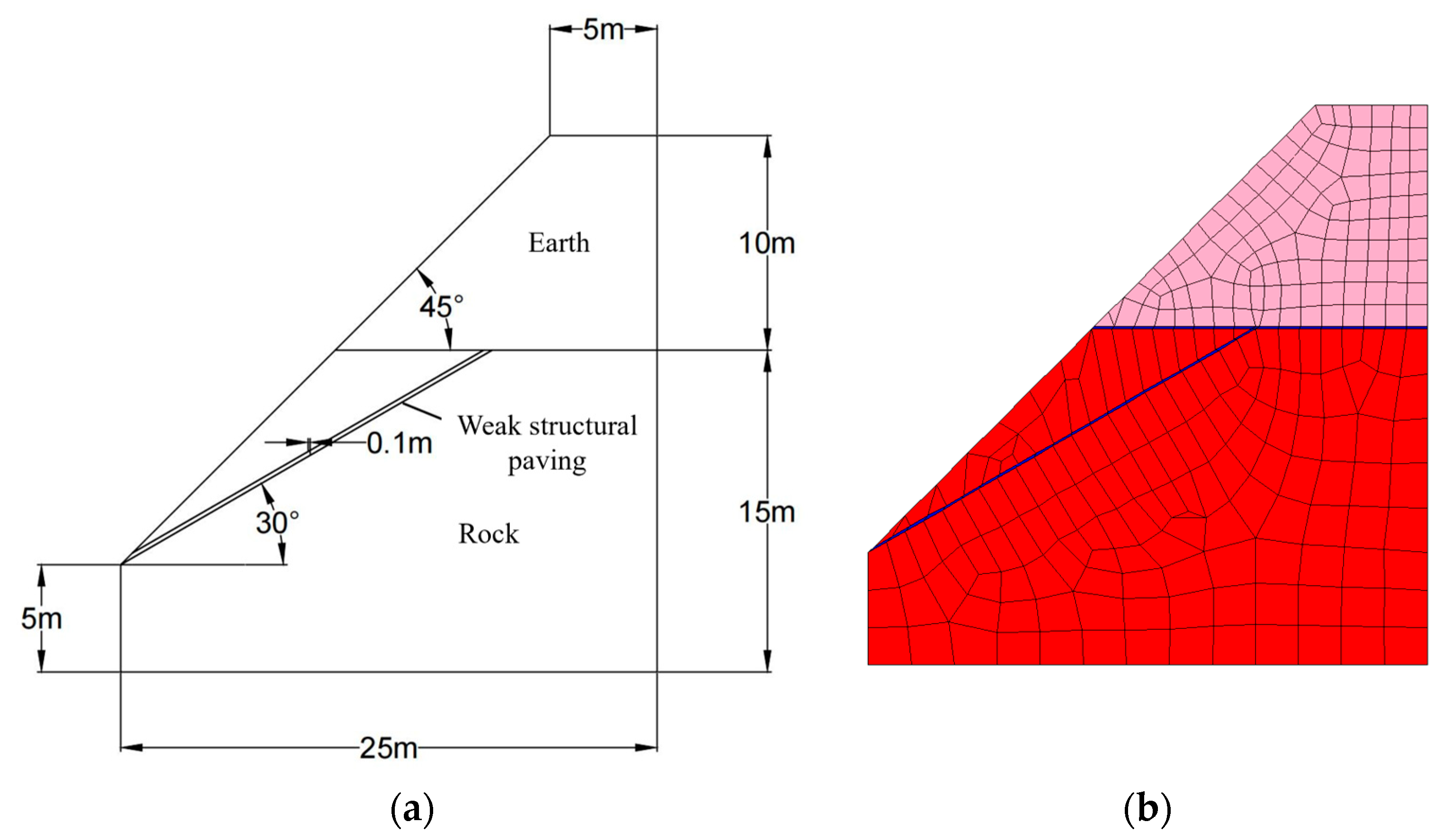
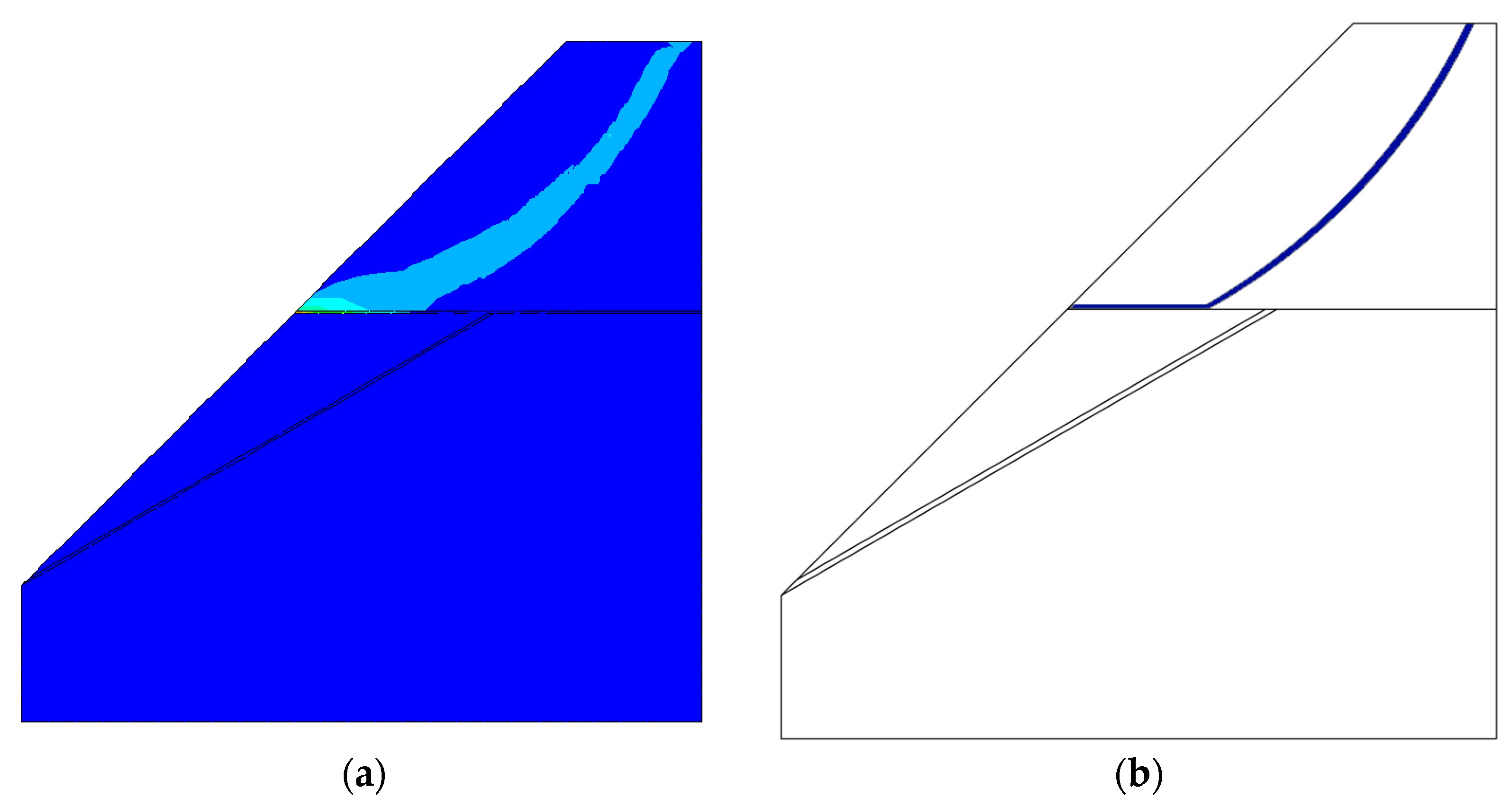
4.4. Example of Slope Stability Analysis of Soil–Rock Binary Structure

The following example illustrates the application of the PRE-IE-FE method to a soil–rock binary structure slope using a straightforward arithmetic approach. This serves as a means of verifying the accuracy of the method in slope stability analysis. The geometric model of the example is illustrated in Figure 4a. It comprises an upper soil body and a lower rock body containing a weak structural surface. The PRE-IE-FE model of the example is illustrated in Figure 4b, where the soil body, rock body, and weak structural surface are partitioned into finite elements, rigid elements, and interface elements, respectively. As the finite elements cannot be directly coupled with the rigid elements through the nodes, the interface elements must also be divided along the soil–rock contact surfaces to ensure the correct transfer of displacements and forces. The rock mass below the slope is considered bedrock, and a fixed constraint is applied to the rigid body element at the center. The slope is only affected by self-weight, and the capacity of the soil–rock contact surface and the weak structural surface is not considered.
The bulk weight of the soil is 18   kN / m 3 , the cohesion is 18   kPa , and the friction angle is 20 ° . The bulk weight of the rock is 2 7   kN / m 3 , the cohesion at the soil–rock contact surface is 2 0   kPa , and the friction angle is 20 ° . The example considers the two instability modes shown in Table 2. The strength parameter of the weak structural surface in the first instability mode is greater than that of the soil, the cohesion is 3 0   kPa , and the friction angle is 29 ° . The strength parameter of the weak structural surface in the second instability mode is less than that of the soil, the cohesion is 1 0   kPa , and the friction angle is 20 ° .
In the first mode of instability, the equivalent plastic strain cloud of the soil–rock binary structure slope is illustrated in Figure 5a, and the schematic of the sliding surface is presented in Figure 5b. Given that the strength parameters of the soil body and the soil–rock contact surface are considerably lower than those of the weak structural surfaces within the rock body, the slope becomes destabilized at the upper soil body. This results in the formation of a composite sliding surface comprising curved sliding surfaces within the soil body and linear sliding surfaces on the soil–rock contact surface, as observed in the slope. Given that the lower rock body is not readily destabilized, it can be regarded as stable bedrock. The soil–rock contact surface, in contrast, is regarded as another layer of thinner soil body with different strength parameters from the upper soil body. This transformation allows the stability problem of soil–rock dichotomous structural slopes to be addressed as a stability problem of two-layer soil slopes. This approach allows for the stability of the slope to be analyzed using the limit equilibrium method, and the stability safety coefficients calculated using PRE-IE-FE can be compared. The results of the safety coefficients calculated using the different methods are presented in Table 3. As can be observed from the table, the results calculated using PRE-IE-FE are in close proximity to those of the three-limit equilibrium bar-splitting methods. This indicates that PRE-IE-FE is an effective method for accurately analyzing the stability of the soil–rock binary structural slopes in the first type of destabilization mode.
In the second mode of instability, the equivalent plastic strain cloud diagram of the soil–rock binary structure slope is presented in Figure 6a, and the schematic diagram of the sliding surface is shown in Figure 6b. Given that the strength parameter of the soil and the soil–rock contact surface is greater than that of the weak structural surface within the rock body, the slope is destabilized at the weak structural surface, resulting in damage to the upper soil body and the formation of a composite sliding surface comprising a curved sliding surface within the soil body and a straight sliding surface on the weak structural surface. In this case, the traditional limit equilibrium method is unable to determine the location of the sliding surface with sufficient accuracy, thereby preventing an accurate calculation of the safety factor. At this juncture, the lower rock body can be regarded as a deformable body, and a finite element mesh is constructed on it. In this case, the lower rock mass is treated as a deformable body, discretized into a finite element mesh. Stability analyses are conducted using the PFE-IE method proposed by Li [11] and the Finite Difference Method (FDM) implemented in the commercial software FLAC. The calculated safety factors are then compared with those obtained from the PRE-IE-FE method. The results of calculating the safety factors using the different methods are presented in Table 4. As can be observed from the table, the calculated safety factor is marginally larger due to PRE-IE-FE’s disregard for the elastic deformation of the lower rock body. Nevertheless, the resulting calculations remain in close proximity to those of PFE-IE and FDM, thereby substantiating PRE-IE-FE’s capacity to accurately analyze the stability of soil–rock binary structure slopes in the second destabilization mode. Additionally, the FLAC calculation for this example required approximately four minutes to complete, given that the PFE-IE method employed a substantial FORTRAN-based program to perform the calculations without utilizing established commercial software. Consequently, a direct comparison of calculation speeds is not feasible. In contrast, the PRE-IE-FE method completed the calculation in less than one minute, which is indicative of the high efficiency of PRE-IE-FE in stability analysis. The aforementioned results demonstrate that PRE-IE-FE is an effective tool for analyzing the stability of soil–rock binary structure slopes in the second destabilization mode. Furthermore, the computational efficiency of PRE-IE-FE is evident, with FLAC requiring approximately four minutes to perform the strength reduction, whereas PRE-IE-FE completed the calculation in less than one minute.
The software used in this paper and its version number and source are shown in Table 5.

5. Conclusions

To address the complexity of instability modes in soil–rock binary structure slopes and the limitations of traditional methods in balancing accuracy and efficiency, this study proposes a coupled numerical approach that integrates the finite element method with the Partitioned Rigid Element–Interface Element–Finite Element (PRE-IE-FE) method. The key findings are summarized as follows:
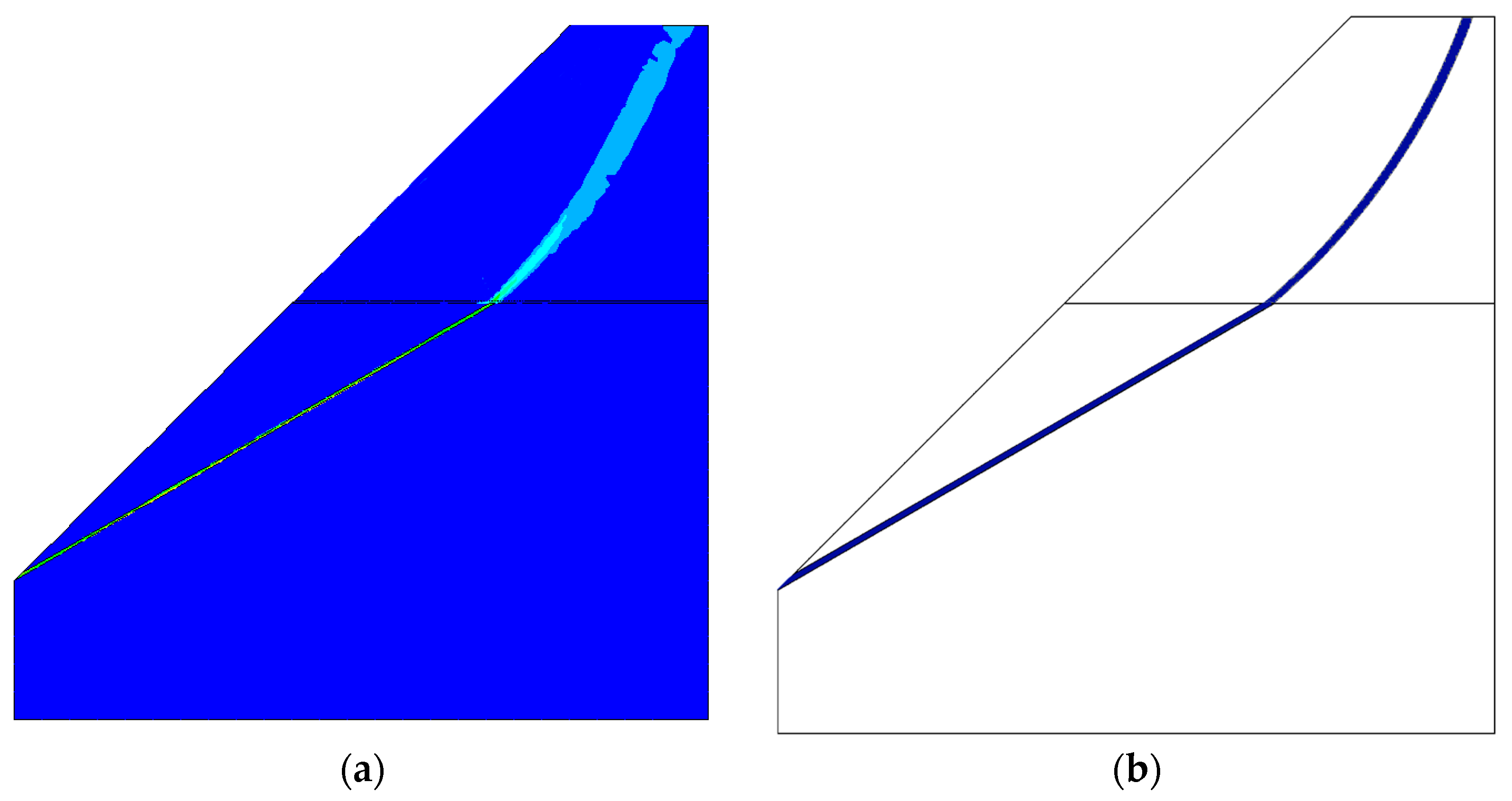
  • Type I slopes (loose soil overlying stable bedrock) exhibit composite failure, involving rotational sliding within the soil and linear sliding along the soil–rock interface. Type II slopes (rock masses containing weak structural surfaces) destabilize via planar sliding along these weak structural surfaces, which drives rotational sliding of the overlying soil and forms composite slip surfaces.
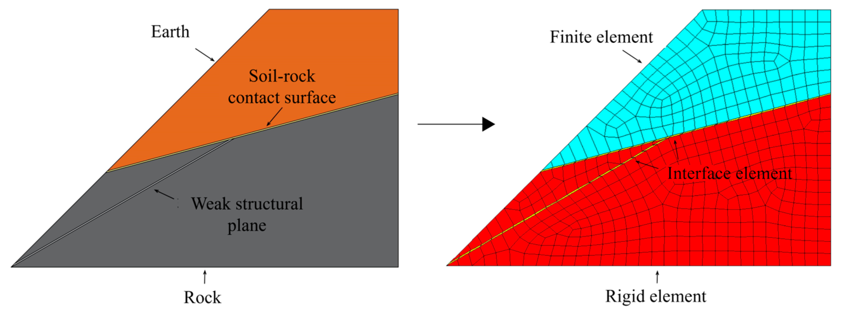
  • The PRE-IE-FE method couples the overlying soil (modeled as a continuous medium using the FEM) and the underlying rock (simulated as discontinuous rigid elements) through interface elements. This framework simultaneously captures soil elastic deformation and rock contact nonlinearity while maintaining computational efficiency.
  • Leveraging ANSYS secondary development and a Python-based hybrid programming framework, a partitioned dynamic stiffness matrix update strategy significantly enhances solving efficiency. Integration with the strength reduction method and a numerical non-convergence criterion enables the rapid determination of safety factors and the visualization of sliding surfaces.
  • The safety factors derived from PRE-IE-FE demonstrate close agreement with results obtained from established methods, such as limit equilibrium analysis and FLAC, confirming the method’s reliability in the stability assessment of soil–rock binary slopes.

6. Limitations and Future Work

6.1. Limitations

  • All case studies are confined to 2D plane-strain conditions. Extending to 3D would require redefining rigid-body degrees of freedom (e.g., six-DOF motion) and implementing hexahedral interface elements, which would significantly increase computational complexity. Additionally, the framework focuses on static equilibrium, excluding dynamic loads (e.g., seismic effects).
  • The method assumes isotropic rock properties, neglecting directional anisotropy (e.g., bedding or joint effects). Furthermore, the displacement compatibility equations for interface elements are derived under small-deformation theory, which may fail to capture geometric nonlinearities in large-displacement scenarios.
  • The numerical robustness of the PRE-IE-FE method is supported by its inheritance of mesh-stable characteristics from the original PRE-IE framework [15], where validation cases (e.g., symmetric wedge models) showed consistent results across mesh refinements, indicating minimal sensitivity to volumetric discretization. However, a dedicated mesh-dependency analysis for soil–rock binary slopes was not performed. Additionally, the small-deformation assumption for interface compatibility limits its applicability to large-displacement scenarios, necessitating future integration of adaptive remeshing or finite deformation theory.

6.2. Future Work

  • Extend the method to 3D spatial and dynamic problems.
  • Incorporate anisotropic strength criteria for structural planes.
  • Conduct comprehensive mesh-dependency and large-deformation analyses.
  • Validate against field monitoring data for practical engineering applications.

Author Contributions

Conceptualization, T.S.; methodology, T.S.; software, Y.P.; validation, B.H., J.W. and Y.P.; formal analysis, Y.P.; investigation, T.S.; resources, J.X.; data curation, J.W.; writing—original draft preparation, T.S.; writing—review and editing, J.X. and B.H.; visualization, Y.P.; supervision, J.X.; project administration, J.X.; funding acquisition, T.S. All authors have read and agreed to the published version of the manuscript.

Funding

This research was funded by National Key Research and Development Program of China grant number [2022YFC3005403]. And The APC was funded by Hohai University.

Institutional Review Board Statement

Not applicable.

Informed Consent Statement

Not applicable.

Data Availability Statement

Restrictions apply to the datasets: The datasets presented in this article are not readily available because the data are part of an ongoing study. Requests to access the datasets should be directed to hhustz@126.com.

Conflicts of Interest

Authors Jianrong Xu, Yu Peng and Jianxin Wang were employed by the company Powerchina Huadong Engineering Corporation Limited. The remaining authors declare that the research was conducted in the absence of any commercial or financial relationships that could be construed as a potential conflict of interest.

References

  1. Ministry of Water Resources of the People’s Republic of China. Design Specification for Slopes of Water Conservancy and Hydropower Projects; SL 386-2007; China Water & Power Press: Beijing, China, 2007.
  2. Sun, W. Study of Instability Mechanism and Intelligent Pre-Warning for Cutting Slope with Soil-Rock Binary Structure. Ph.D. Thesis, Chang’an University, Xi’an, China, 2020. [Google Scholar] [CrossRef]
  3. Wei, Y.; Qiu, Y. A Brief Analysis of Road Slope Classification Based on Damage Mechanism and Damage Mode. China Investig. Des. 2019, 2, 80–82. [Google Scholar]
  4. Kou, R. Identification and Determination of Potential Slip Surfaces on Binary Structure Slopes. Ph.D. Thesis, Kunming University of Science and Technology, Kunming, China, 2016. [Google Scholar]
  5. Tang, X.; Zheng, Y.; Tang, H. Numerical Analysis on the Evolutionary Features of Deformation and Failure Modes of Slope. Appl. Mech. Mater. 2012, 204, 144–154. [Google Scholar] [CrossRef]
  6. Zhao, L.; Li, T.; Niu, Z. A Mixed finite element method for contact problems with friction and initial gaps. Chin. J. Geotech. Eng. 2006, 28, 2015–2018. [Google Scholar]
  7. Li, T.; Liu, X.; Zhao, L. An interactive method of interface boundary elements and partitioned finite elements for local continuous/discontinuous deformation problems. Int. J. Numer. Methods Eng. 2014, 100, 534–554. [Google Scholar] [CrossRef]
  8. Ren, Q. Rigid Body Element Method and Its Application in Stability Analysis of Rock Mass. J. Hohai Univ. (Nat. Sci.) 1995, 23, 1–7. [Google Scholar]
  9. Ren, Q.; Yu, T. Theory and calculating model of block element method. Eng. Mech. 1999, 16, 67–77. [Google Scholar]
  10. Zhuo, J. Interface Element Method for Mechanical Problems in Discontinuous Media; Science Press: Beijing, China, 2000. [Google Scholar]
  11. Zhang, Q.; Zhuo, J. Interface element method and criterion for stability analysis of high slopes in three gorges shiplock. Chin. J. Rock Mech. Eng. 2000, 19, 285–288. [Google Scholar]
  12. Qi, H.; Li, T.; Liu, X.; Zhao, L.; He, J.; Li, X. A fast local nonlinear solution technique based on the partitioned finite element and interface element method. Int. J. Numer. Methods Eng. 2022, 123, 2214–2236. [Google Scholar] [CrossRef]
  13. Fan, S.; Li, T.; Liu, X.; Zhao, L.; Niu, Z.; Qi, H. A hybrid algorithm of partitioned finite element and interface element for dynamic contact problems with discontinuous deformation. Comput. Geotech. 2018, 101, 130–140. [Google Scholar] [CrossRef]
  14. Li, T.; He, J.; Zhao, L.; Li, X.; Niu, Z. Strength reduction method for stability analysis of local discontinuous rock mass with iterative method of partitioned finite element and interface boundary element. Math. Probl. Eng. 2015, 2015, 872834. [Google Scholar] [CrossRef]
  15. Sheng, T.; Li, T.; Liu, X.; Qi, H. A partitioned rigid-element and interface-element method for rock-slope-stability analysis. Appl. Sci. 2023, 13, 7301. [Google Scholar] [CrossRef]
  16. Wu, S. Stability Analyses and Mitigation Measures of Typical Slopes in Zhao-Yin Expressway. Soil Eng. Found. 2013, 27, 29–31. [Google Scholar]
  17. Zhang, L.; Tang, L.; Luo, K. Stability Analysis for Soil-Rock Composite Slope. Geotech. Eng. Tech. 2008, 22, 119–122. [Google Scholar]
  18. Zhu, D. Revival Mechanism and Deformation Prediction of Typical Accumulative Landslide in the Three Gorges Reservoir. Ph.D. Thesis, China University of Geosciences, Wuhan, China, 2010. [Google Scholar]
  19. Zou, D.; Zheng, H. Fast Lagrangian Method and Its Applications in Slope Stability Analysis. Min. Res. Dev. 2005, 25, 80–83. [Google Scholar] [CrossRef]
  20. Zhao, L.; Li, T.; Yang, Q. Numerical simulation method for instability motion and initial surge of soil bank slopes under earthquake action. J. Hydroelectr. 2011, 30, 104–108. [Google Scholar]
  21. Cheng, L.; Liu, Y.; Yang, Q.; Pan, Y.; Lv, Z. Mechanism and numerical simulation of reservoir slope deformation during impounding of high arch dams based on nonlinear FEM. Comput. Geotech. 2017, 81, 143–154. [Google Scholar] [CrossRef]
  22. Lin, C.; Li, T.; Zhao, L.; Zhang, Z.; Lin, C.; Liu, X.; Niu, Z. Reinforcement effects and safety monitoring index for high steep slopes: A case study in China. Eng. Geol. 2020, 279, 105861. [Google Scholar] [CrossRef]
  23. Su, Z.; Shao, L. Three-dimensional slope stability based on the finite element limit equilibrium method. Chin. J. Eng. 2022, 44, 2048–2056. [Google Scholar] [CrossRef]
  24. Yan, Q.; Lian, X.; Ling, J. Time series finite element analysis of support of slope excavation. J. Traffic Transp. Eng. 2020, 20, 61–71. [Google Scholar] [CrossRef]
  25. Wang, X. Finite Element Method; Tsinghua University Press: Beijing, China, 2003. [Google Scholar]
  26. Shi, F. ANSYS Secondary Development and Application Examples in Detail; China Water & Power Press: Beijing, China, 2012. [Google Scholar]
Figure 1. Partitioned Rigid Element–Interface Element–Finite Element model for soil–rock binary structure slope.
Applsci 15 04903 g001
Figure 2. Schematic diagram of the coupled interface elements between finite element and rigid body elements.
Applsci 15 04903 g002
Figure 3. Computational flow of Partitioned Rigid Body Element–Interface Element–Finite Element procedure.
Applsci 15 04903 g003
Figure 4. (a) Geometric modeling of slopes with soil–rock binary structures. (b) PRE-IE-FE modeling of slopes with soil–rock binary structures.
Applsci 15 04903 g004
Figure 5. (a) Equivalent plastic strain maps of slopes with soil–rock binary structure (first instability model). (b) Schematic diagram of slope sliding surface of soil–rock binary structure (first destabilization model).
Applsci 15 04903 g005
Figure 6. (a) Equivalent plastic strain maps of slopes with soil–rock binary structure (second instability mode). (b) Schematic diagram of the sliding surface of an earth–rock binary structure slope (second destabilization model).
Applsci 15 04903 g006
Table 1. Types of slopes with soil–rock binary structures.
Criteria for ClassificationTypologyNote
Morphology of soil–rock contact surfacesLinear contact surface typeThe shape of the soil–rock contact surface is straight
Folded contact surface typeThe shape of the soil–rock contact surface is folded
Arc contact surface typeThe shape of the soil–rock contact surface is curved
Irregular contact surface typeIrregular shape of soil–rock contact surfaces
Properties of soil–rock contact surfacesHorizontal contact surface typeApproximate level of soil–rock contact surface
Gently tilting contact surface typeSoil–rock contact surface angle < Integrated slope angle for slopes
Steeply inclined contact surface typeSoil–rock contact surface angle ≥ Integrated slope angle for slopes
Anti-dumping contact surface typeSoil–rock contact surface inclination is opposite to slope inclination
Oblique contact surface typeSoil–rock contact surface inclination at an angle to the slope inclination
Tendency of the top face of the slopeTop climbing typeSlope top surface inclination is the same as the slope inclination
Flat-toppedThe top surface of the slope is approximately horizontal
Top downhill typeThe slope top surface tends to be the opposite of the side slope tendency
Thickness of claddingThin layer coverage typeCladding thickness < 10 m
Medium-thickness cover type10 m ≤ Cladding thickness < 20 m
Thick cover typeCladding thickness ≥ 20 m
Number of steps in overburden excavationSingle-stage coverage typeThe number of steps in the overburden excavation is 1
Two-stage coverage typeThe number of steps in the overburden excavation is 2
Multi-level coverage typeThe number of steps in the overburden excavation is >2
Table 2. Two common and easily destabilized soil–rock binary structural slope types.
Slope StructureSlope ModelingDestabilization ModeSliding Surface Pattern
Upper portion is stockpiled soil
Stable bedrock below
Applsci 15 04903 i001Applsci 15 04903 i002Applsci 15 04903 i003
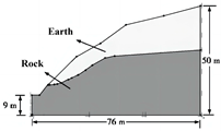
The upper part is an accumulation of soil
or fully weathered rock
Lower part is a rock body with weak structural surfaces
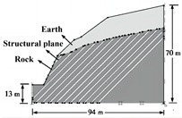
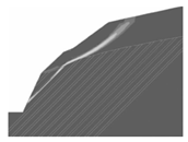
Applsci 15 04903 i004Applsci 15 04903 i005Applsci 15 04903 i006
Table 3. Coefficients of safety calculated using different methods for the first instability mode of soil–rock binary structure slopes.
MethodologiesPRE-IE-FESimplified Bishop MethodJanbu MethodMorgenstern–Price Method
safety factor0.8320.8330.8250.829
Table 4. Coefficients of safety calculated using different methods for the second destabilization mode of soil–rock binary structure slopes.
EthodologiesPRE-IE-FEPFE-IEFDM
safety factor1.2851.2551.272
computation time<1 min——4 min
Table 5. Computational Environment Configuration: Software Packages, Version Specifications, and Sources.
SoftwareVersionOrganization/Source
Python3.9Python Software Foundation, https://www.python.org
Ansys Mechanical2020 R1Ansys Inc., Canonsburg, PA, USA
PyMAPDL0.63.2PyPI, https://pypi.org/project/ansys-mapdl-core/ (accessed on 29 March 2025).
PyVista0.42.0PyPI, https://pypi.org/project/pyvista/ (accessed on 29 March 2025).
FLAC1.4.3Xiph Foundation, https://xiph.org/flac/ (accessed on 29 March 2025).
Disclaimer/Publisher’s Note: The statements, opinions and data contained in all publications are solely those of the individual author(s) and contributor(s) and not of MDPI and/or the editor(s). MDPI and/or the editor(s) disclaim responsibility for any injury to people or property resulting from any ideas, methods, instructions or products referred to in the content.

