HFDF-EffNetV2: A Lightweight, Noise-Robust Model for Fault Diagnosis in Rolling Bearings

Abstract

In rolling bearing intelligent fault diagnosis (FD), lightweight models are constrained by issues such as noise interference and the scarcity of fault data, making it challenging to achieve real-time, high-accuracy diagnosis on resource-limited devices. To address these challenges, this study proposes a lightweight model that combines the hierarchical fine-grained decision fusion (HFDF) strategy with an improved EfficientNetV2 architecture (HFDF-EffNetV2). The model optimizes depth and width multiplicity factors to enhance parameter utilization efficiency. It uses pyramidal convolution (PyConv) combined with Fused-MBConv (Fused-MBPyConv) to obtain multi-scale time-frequency information. Additionally, an enhanced MBConv, termed BSMB-Conv-MLCA, integrates subspace blueprint separable convolution (BSConv-S) with mixed local channel attention (MLCA) extract deep-grained fault features. The HFDF strategy outputs confidence in stages and updates weights to prevent the model from falling into local overfitting when handling confusable samples. Experimental results on Case 1 and Case 2 show that HFDF-EffNetV2 achieved 100% accuracy with diagnostic times of 18.67 millisecond (ms) and 17.56 ms, respectively, and 1.85 million (M) parameters. Under noisy conditions, average accuracies reached 98.19% and 85.68%, respectively. Additionally, the model performed well with small samples, yielding accuracies of 98.69% and 97.51%. These results highlight its superior robustness to noise and lightweight performance compared with other advanced models.

1. Introduction

Rolling bearings, which are crucial components of mechanical equipment, are prone to various types of damage due to their long running time and harsh working environment [1]. If damaged components cannot be detected and replaced promptly, outcomes include disruption of the normal operation of the mechanical equipment, lower production efficiency, and even serious consequences such as substantial economic losses and casualties [2]. Accurate, real-time detection and diagnosis of the operating condition of rolling bearings is therefore essential [3].

In fault diagnosis (FD), vibration signals are widely used as effective diagnostic signals due to their ability to quickly and accurately reflect equipment operating conditions [4,5,6]. Traditional FD methods mainly rely on signal-decomposition techniques such as feature mode decomposition [7], all time-scale decomposition [8] and Blaschke mode decomposition [9]. These methods identify fault types by analyzing the characteristics of the vibration signal, but they heavily rely on empirical knowledge and are difficult to interpret for people without relevant expertise [10]. Compared to signal-decomposition methods, deep learning techniques have been more widely researched and applied in industry because they do not require a priori knowledge and have superior feature-extraction capability [11,12]. For instance, Chang et al. [13] proposed an FD model combining a one-dimensional convolutional neural network (CNN) with a two-dimensional improved ResNet-50, which utilizes multi-modal information to enhance the robustness of the model. Han et al. [14] proposed the MT-ConvFormer FD model, which utilizes multi-task learning to extract fault information. Song et al. [15] proposed an FD model based on multimodal data fusion and the subtraction-average-based optimizer to address the challenge of poor model generalization with small samples by combining CNN and support vector machines. Although these approaches effectively improve FD results by introducing various mechanisms, they also require extensive parameter calculations, leading to increased consumption of storage and computational resources.

In recent years, the rapid development of embedded components and digital twin technology have provided new solutions for FD in rolling bearings in special operating scenarios [16]. Due to the advantages of edge computing, such as fast transmission and low latency, the lightweight FD methods for rolling bearings have attracted significant attention in recent research [17]. To enable real-time diagnosis, Fan et al. [18] proposed a lightweight, multi-scale, multi-attention feature fusion network that significantly enhances fault feature identification. Wang et al. [19] proposed an AUTO-CNN architectural design method, aiming to achieve a balance between accuracy and use of computational resources. Teta et al. [20] designed a lightweight CNN and fine-tuned it using the energy-valley optimizer. Wang et al. [21] proposed a lightweight FD model that integrates frequency-slice wavelet transform with an improved neural-transformer that emphasizes the global capture of important fine-grained information. Xie et al. [22] designed a lightweight pyramid attention residual network for fault diagnosis under changing operating conditions. However, while the above methods have the advantages of their light weights and the promising results they achieve through different technical approaches, they are over-reliant on global information and neglect to utilize the information extracted at different stages for a more comprehensive diagnosis. Although lightweight models offer advantages such as low computational cost and high diagnostic speed, they face several challenges in practical applications. For instance, issues such as limited fault data and noise interference in real-world scenarios significantly hinder the practical deployment of lightweight models [23,24,25,26].

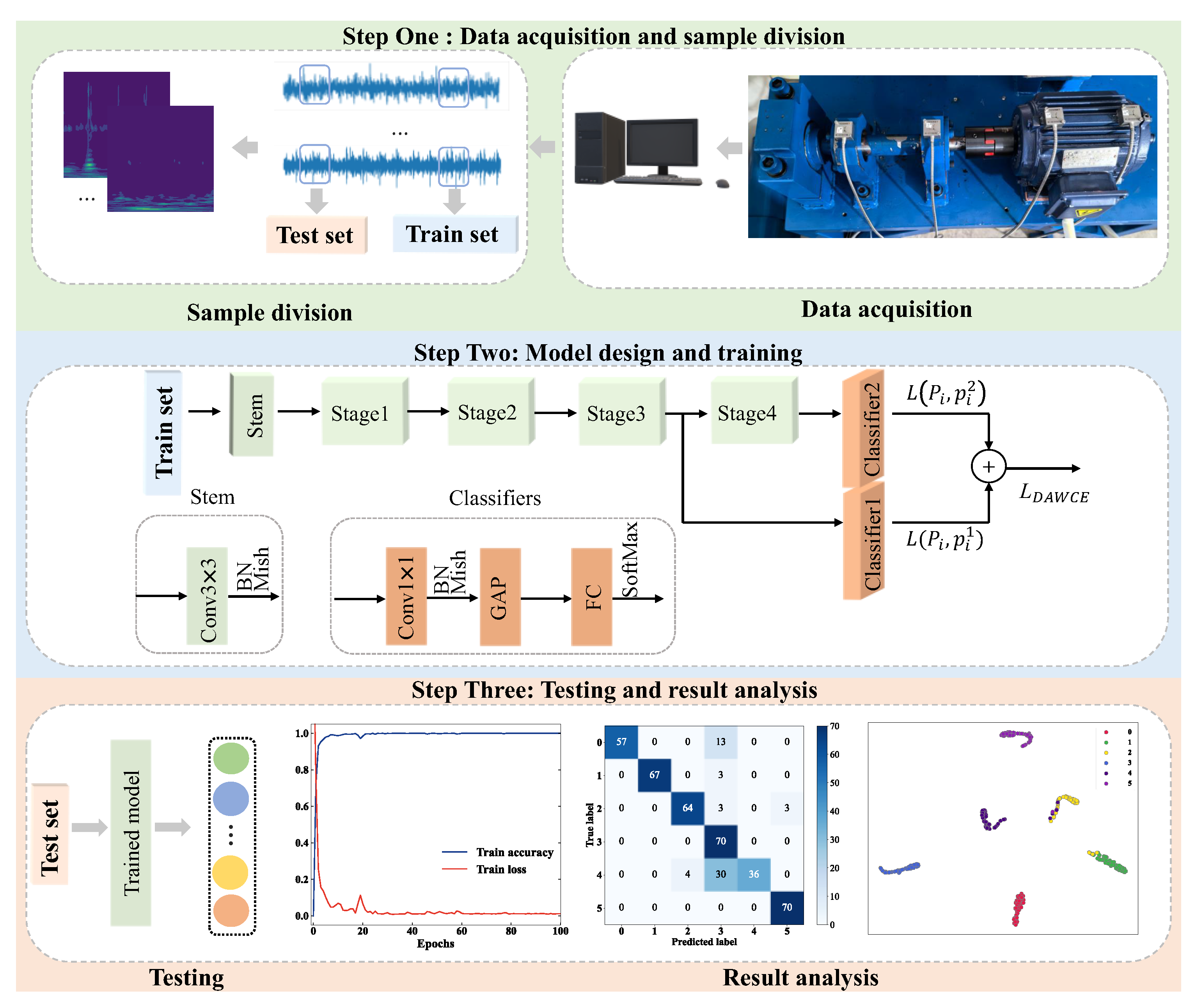
Aiming to address the challenges of achieving light weight, high accuracy, strong robustness to noise, and real-time responsiveness in practical industrial applications, we propose HFDF-EffNetV2, a lightweight FD model, with the following main contributions:

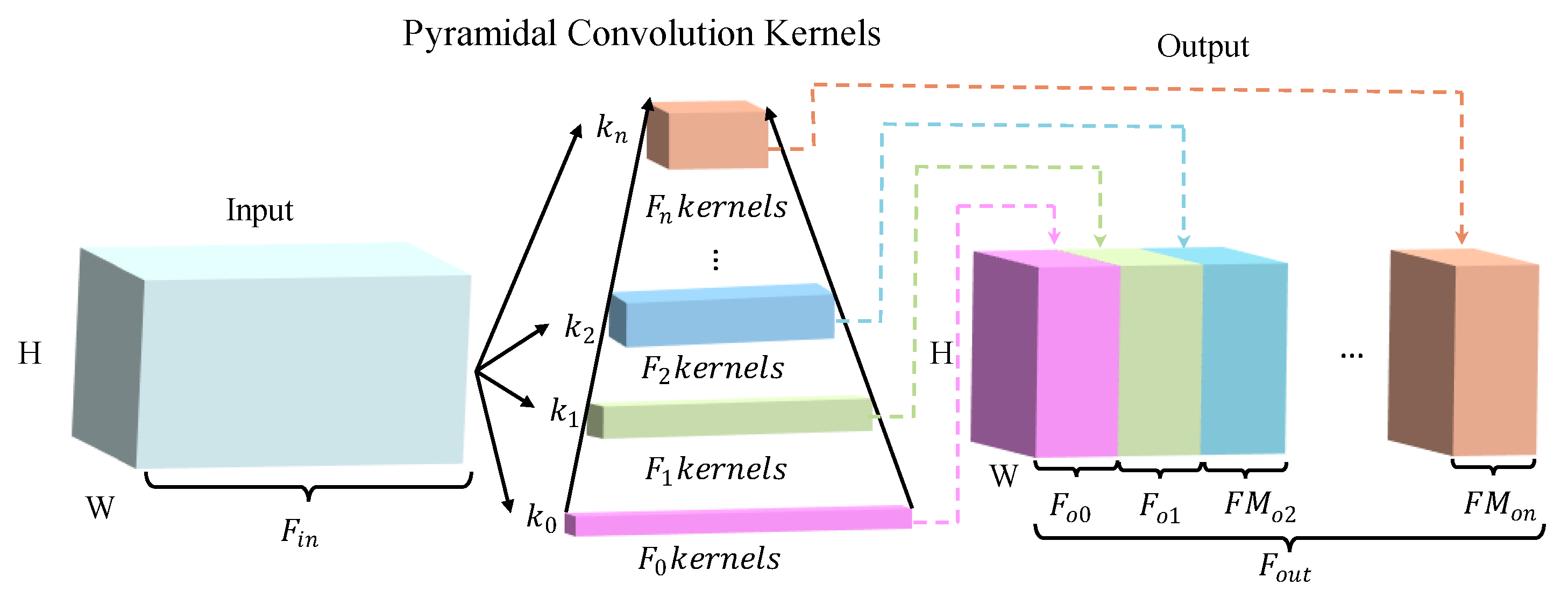
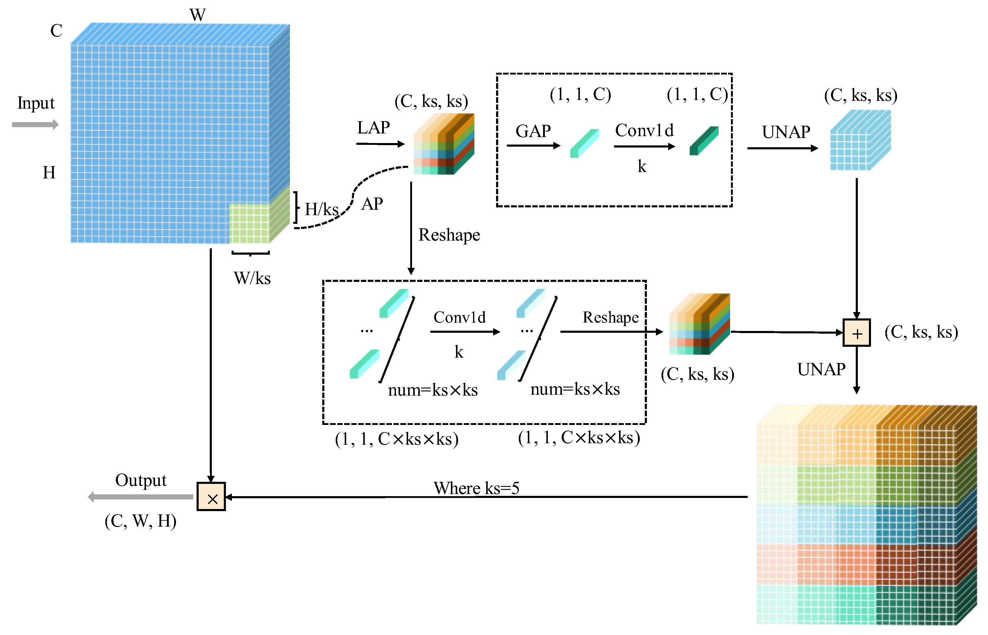
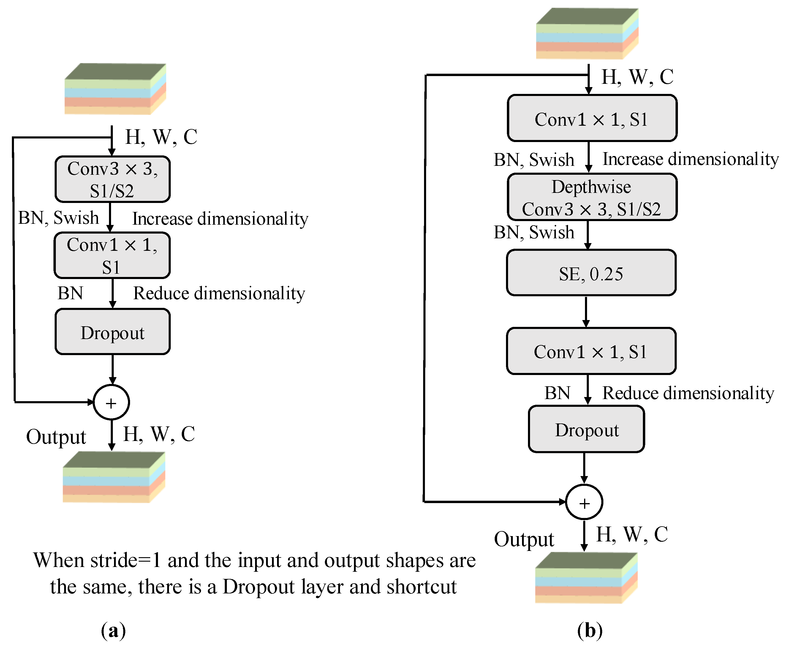
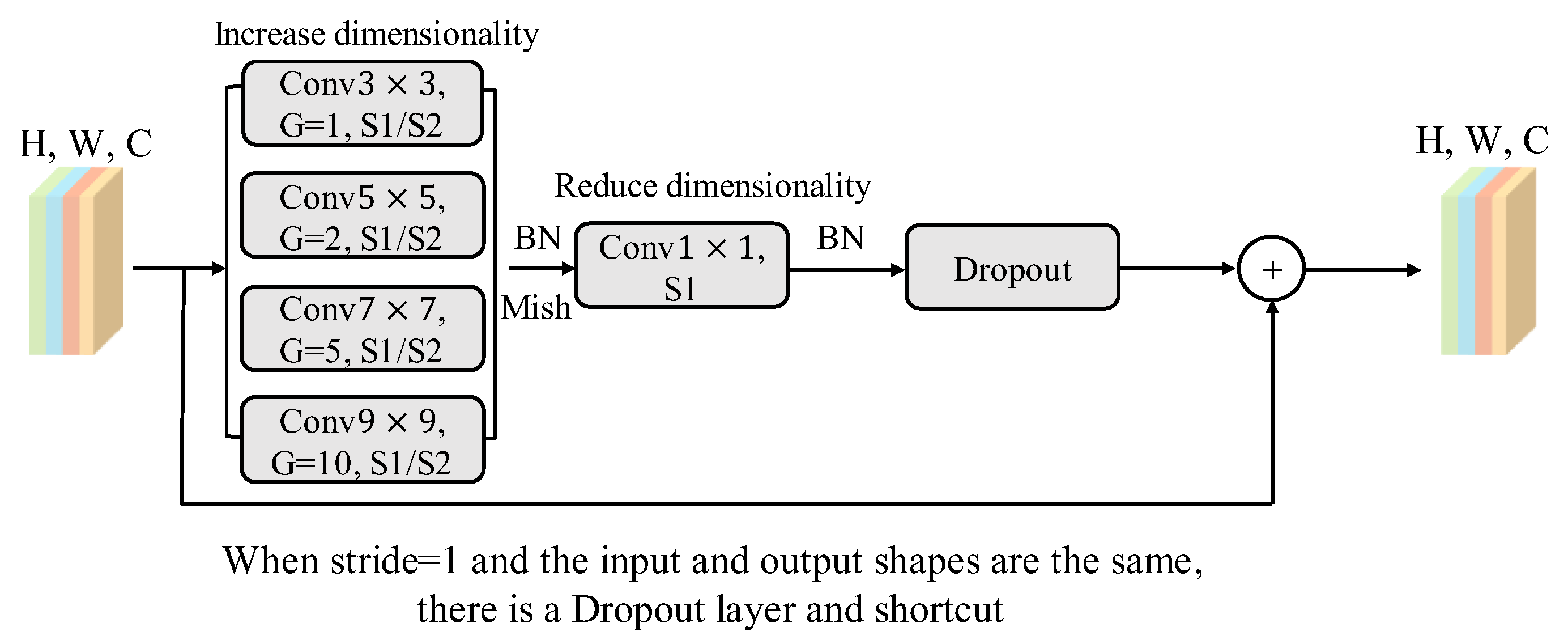
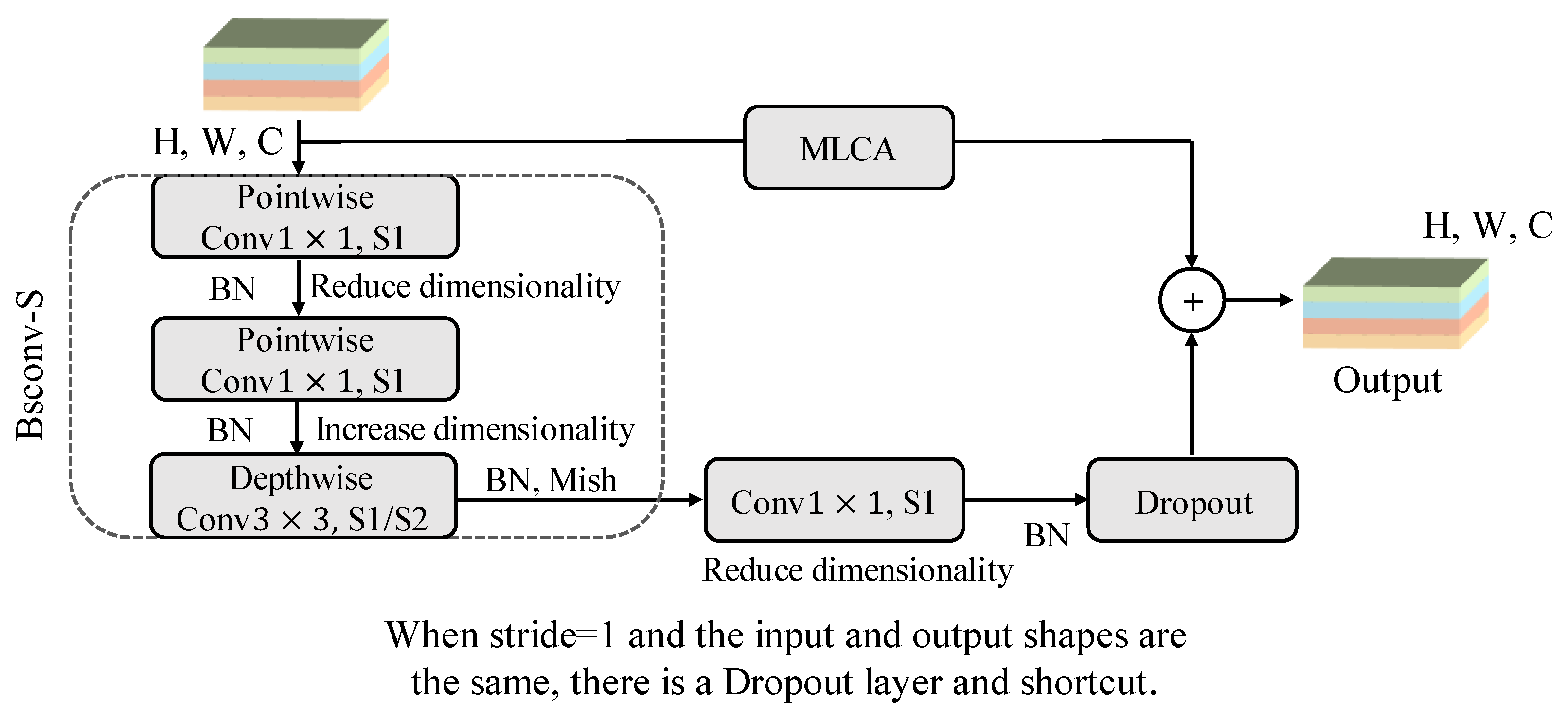
• The improved EfficientNetV2 was constructed based on multiplicity factors combined with the Mish activation function. Additionally, Fused-MBPyConv and BSMBConv-MLCA were designed to combine multi-scale shallow features with multi-dimensional deep features for efficient extraction of representative fault features from time-frequency feature maps (FMs).
• The hierarchical fine-grained decision fusion (HFDF) strategy is proposed to perform weight updating in phases to alleviate the tendency of the lightweight model to fall into local overfitting when dealing with confusable fault types and small samples.

The proposed model was evaluated under noisy and small-sample conditions and compared with six other models. The results indicate that the proposed model outperforms these others in terms of robustness to noise and stability while remaining lightweight.

The remainder of this study is structured as follows. Section 2 presents the materials and methods; Section 3 describes the results, providing detailed architectural parameters; Section 4 discusses the robustness to noise and stability of HFDF-EffNetV2 in two cases; Section 5 concludes this study.

2. Materials and Methods

2.1. Continuous Wavelet Transform

In a rolling-bearing FD task, a fault signal from monitored equipment is easily lost in noise due to vibrations from the equipment and environmental factors; this noisiness increases the difficulty of later feature extraction [27]. The continuous wavelet transform (CWT) provides rich time-frequency information, which more effectively highlights the fault characteristics of the target components [28]. Considering the limited computational resources of edge devices, this study employed the CWT to convert the signals into time-frequency FMs with a resolution of $128\times 128\times 3$; the FMs were then used as fault samples. The CWT is calculated as shown in Equation (1):

$$\mathrm{CWT}(\mathrm{a},\mathrm{b})={\displaystyle \frac{1}{\sqrt{\mathrm{a}}}}{\int }_{-\infty }^{\infty }\mathrm{x}(\mathrm{t}){\mathsf{\psi }}^{*}({\displaystyle \frac{\mathrm{t}-\mathrm{b}}{\mathrm{a}}})\mathrm{dt}$$

(1)

where $\mathrm{x}(\mathrm{t})$ is the input signal, ${\mathsf{\psi }}^{*}(\mathrm{t})$ is the complex conjugate of the scaled and shifted wavelet function $\mathsf{\psi }(\mathrm{t})$, $\mathrm{a}$ is the scale factor, and $\mathrm{b}$ is the translation factor.

2.2. Pyramidal Convolution

Due to the limited receptive field of a single convolutional kernel, when the feature information in the time-frequency FM is located at the edges, small convolutional kernels are not sufficiently sensitive to edge information, resulting in the loss of edge details. Although large convolutional kernels have a larger receptive field, they require a substantial increase in parameters. As shown in Figure 1, pyramidal convolution (PyConv) comprises convolutional kernel of varying sizes, with the kernel sizes gradually increasing from bottom to top. In addition, PyConv introduces the grouped convolution. The input FMs are then processed through grouped convolution and subsequently fused into a complete output FM along the channel dimension. Compared to atrous spatial pyramid pooling, which utilizes the dilated convolution technique, PyConv offers superior feature capture capabilities and demonstrates better computational efficiency [29].

2.3. Subspace Blueprint Separable Convolution

Haase et al. [30] visualized the convolutional kernels of VGG-19, InceptionV2, and ResNet-50 and found that many FMs were linearly transformed by a special convolution kernel, referred to as the ‘Blueprint’, demonstrating intra-kernel correlation. Building on this concept, the authors propose the subspace blueprint separable convolution (BSConv-S), which effectively suppresses irrelevant features in the convolution operation through a subspace separation mechanism. In BSConv-S, the convolution process consists of three sub-processes, as follows:

• The input tensor $\mathrm{X}$ is mapped to an ${\mathrm{M}}^{\prime }$-dimensional subspace by $\mathrm{M}$ pointwise convolutional kernels of size $1\times 1$$({\mathsf{\omega }}_1^{\mathrm{B}},{\mathsf{\omega }}_2^{\mathrm{B}},\dots ,{\mathsf{\omega }}_{{\mathrm{m}}^{\prime }}^{\mathrm{B}},\dots ,{\mathsf{\omega }}_{{\mathrm{M}}^{\prime }}^{\mathrm{B}})$, compressing the number of channels.
• Another $\mathrm{N}$ pointwise convolutional kernels of size $1\times 1$$({\mathsf{\omega }}_1^{\mathrm{A}},{\mathsf{\omega }}_2^{\mathrm{A}},\dots ,{\mathsf{\omega }}_{\mathrm{n}}^{\mathrm{A}},\dots ,{\mathsf{\omega }}_{\mathrm{N}}^{\mathrm{A}})$ are applied to the result of step 1.
• Finally, $\mathrm{N}$ depthwise separable convolutional kernels of size $\mathrm{k}\times \mathrm{k}$$({\mathrm{B}}_1,{\mathrm{B}}_2,\dots ,{\mathrm{B}}_{\mathrm{n}},\dots ,{\mathrm{B}}_{\mathrm{N}})$ are applied to the results of step 2.

The computational relationship between the input tensor $\mathrm{X}$ and the output tensor $\mathrm{Y}$ is shown in Equation (2) as follows:

$${\mathrm{Y}}_{\mathrm{n},\text{:},\text{:}}=\mathrm{X}\times {\mathsf{\omega }}_{{\mathrm{M}}^{\prime }}^{\mathrm{B}}\times {\mathsf{\omega }}_{\mathrm{n}}^{\mathrm{A}}\times {\mathrm{B}}_{\mathrm{n}},\mathrm{n}=1,\dots ,\mathrm{N}$$

(2)

2.4. Mixed Local Channel Attention Mechanism

Although attention mechanisms like squeeze-and-excitation (SE) and the convolutional block attention module have shown good performance in many tasks, the mixed local channel attention (MLCA) mechanism excels at capturing high-level feature representations. It offers better adaptability and enables more detailed channelwise feature learning across multiple levels, particularly when handling complex features [31]. It applies two steps of average pooling (AP) to transform the input feature vectors into a shape of $(1\times \mathrm{C}\times \mathrm{ks}\times \mathrm{ks})$, with the first branch capturing global information and the second branch capturing local spatial information. After one-dimensional convolution, the two one-dimensional vectors are restored to their original resolution through unaverage pooling (UNAP) and the information is then fused to achieve hybrid attention. As shown in Figure 2, Conv1d denotes one-dimensional convolution, and the kernel size $\mathrm{k}$ of the one-dimensional convolution in MLCA is proportional to the channel $\mathrm{C}$, indicating that only the relationship between each channel and its $\mathrm{k}$ neighboring channels are considered when capturing local cross-channel interaction information. The value of $\mathrm{k}$ is calculated as in Equation (3).

$${\mathrm{k}=\mathsf{\Phi }(\mathrm{C})=\left|{\displaystyle \frac{\mathrm{lo}{\mathrm{g}}_2(\mathrm{C})}{\mathsf{\gamma }}}+{\displaystyle \frac{\mathrm{d}}{\mathsf{\gamma }}}\right|}_{ \mathrm{odd}}$$

(3)

where $\mathrm{C}$ is the number of channels; $\mathrm{k}$ is convolutional kernel size; $\mathsf{\gamma }$ and $\mathrm{d}$ are hyperparameters, with the default value set to 2; the function $\mathrm{odd}$ ensures that $\mathrm{k}$ is odd by adding 1 if $\mathrm{k}$ is even.

2.5. EfficientNetV2

In the field of FD, accuracy is a crucial metric; therefore, while pursuing a lightweight design, it is essential to ensure high diagnostic accuracy, especially in the context of complex tasks [32,33,34].

EfficientNetV2 is a lightweight model introduced by Tan et al. [35] in 2021 that incorporates the Fused-MBConv and MBConv layers and is available in several versions, including B0~B3, S, and M. The model employs a progressive learning strategy that adaptively adjusts the regularization technique and the input image size, accelerating the training process while maintaining high accuracy. Through neural-architecture search, EfficientNetV2 optimizes three key parameters: input-image resolution, network depth, and channel width. Among the different versions, the M version, with depth and width scaling factors of 1.8 and 1.4, respectively, is suited for high-resolution scenarios, achieving a classification accuracy of 85.1% on the ImageNet dataset. In contrast, the S version, with depth and width scaling factors of 1.2 and 1.1, respectively, focuses more on balancing the number of parameters with accuracy, making it more suitable for lower-resolution applications.

EfficientNetV2-S is structured into seven stages; this is one MBConv stage fewer than the M version, resulting in a significant reduction in the number of parameters. As shown in the

Table 1. EfficientNetV2-S architecture.

Stage	Operator	Stride	Channels	Layers
0	Conv$3\times 3$	2	24	1
1	Fused-MBConv$1^1,\mathrm{k}3\times 3$	1	24	2
2	Fused-MBConv$4,\mathrm{k}3\times 3$	2	48	4
3	Fused-MBConv$4,\mathrm{k}3\times 3$	2	64	4
4	MBConv4, $\mathrm{k}3\times 3$, SE0.25	2	128	6
5	MBConv6, $\mathrm{k}3\times 3$, SE0.25	1	160	9
6	MBConv6, $\mathrm{k}3\times 3$, SE0.25	2	256	15
7	Conv$1\times 1$ & Pooling & FC	-	1280	1

¹ The digit following “MBConv” denotes the expansion factor of the input channel.

, stage zero consists of a standard convolutional layer. As illustrated in Figure 3a, stages one to three employ the Fused-MBConv layer, which utilizes $3\times 3$ convolution for channel upscaling, followed by $1\times 1$ convolution for downscaling. In contrast, stages four to six utilize the MBConv layer, as shown in Figure 3b. It begins by introducing features into a higher-dimensional space through $1\times 1$ convolution, and this step is followed by feature extraction with a 3 × 3 depthwise convolution. Subsequently, the SE Attention mechanism is applied to capture significant channelwise features. Finally, a 1 × 1 convolution maps the processed features back to the input space. The final stage includes a 1 × 1 convolutional layer, an AP layer, and a fully connected (FC) layer. This streamlined architecture contributes to its reduced parameter count while maintaining efficient performance.

3. Results

The FD process of HFDF-EffNetV2 is shown in Figure 4. First, the vibration signals collected by the sensors during the machinery operation are transmitted to the digital device. Subsequently, data preprocessing using the CWT is applied to obtain time-frequency FM, which are then divided into training and test sets. The model-training process outputs the predicted probabilities in stages, computes the loss using the dynamic adaptive weighted cross-entropy (DAWCE) function during forward propagation, and updates the weights via backpropagation. Finally, the test set is fed into the trained model for diagnosis, and the diagnostic results are visualized and analyzed from multiple perspectives.

3.1. HFDF-EffNetV2

HFDF-EffNetV2 is constructed by optimizing the depth and width multiplicity factors of EfficientNetV2-S according to the resolution of the input time-frequency FM. In addition, the Mish [36] activation function is employed to enhance gradient flow, thereby improving model training stability. The Mish activation function is calculated as in Equation (4), below:

$$\mathrm{Mish}(\mathsf{\delta })=\mathsf{\delta }\times \tanh (\ln (1+{\mathrm{e}}^{\mathsf{\delta }}))$$

(4)

where $\mathsf{\delta }$ is the input value and $\tanh$ is the hyperbolic tangent function that maps the result to the range $(-1,1)$.

3.1.1. Improving Fused-MBConv with PyConv

EfficientNetV2 introduces Fused-MBConv due to the limited hardware acceleration support for depthwise separable convolutions. Replacing all layers with Fused-MBConv increases the computational overhead of the network; therefore, it is used only in the shallow stages of the model.

To enlarge the receptive field in the shallow stages and capture multiscale feature information, this study constructed Fused-MBPyConv based on combining Fused-MBConv with PyConv, as shown in Figure 5. When the expansion rate is not 1, Fused-MBPyConv first expands the number of input channels using PyConv. A convolutional kernel of size 1 is then applied to map the expanded features to the desired number of output channels. Finally, the residual connection is introduced to enhance feature representation, prevent information loss, and mitigate the vanishing gradient problem. The specific implementation is given by Equation (5). The input FMs are assumed to be $\mathrm{X}\in {\mathrm{R}}^{\mathrm{C}\times \mathrm{H}\times \mathrm{W}}$, where $\mathrm{C}$, $\mathrm{H}$, and $\mathrm{W}$ denote the channel dimension, height, and width of the input FM, respectively.

$$\left\{\begin{array}{c}{\mathrm{F}}_{\mathrm{i}}=\mathrm{C}\mathrm{o}\mathrm{n}\mathrm{v}({\mathrm{ks}}_{\mathrm{i}}\times {\mathrm{ks}}_{\mathrm{i}}{,\mathrm{G}}_{\mathrm{i}}){(\mathrm{X}}_{\mathrm{i}})\in {\mathrm{R}}^{{\displaystyle \frac{\mathrm{C}}{4}}\times \mathrm{H}\times \mathrm{W}}\\ {\displaystyle \genfrac{}{}{0pt}{}{\mathrm{F}=[{\mathrm{F}}_0;{\mathrm{F}}_1;{\mathrm{F}}_2;{\mathrm{F}}_3]\in {\mathrm{R}}^{(\mathrm{E}\times \mathrm{C})\times \mathrm{H}\times \mathrm{W}}}{\mathrm{Y}=\mathrm{Conv}(\mathrm{F})\in {\mathrm{R}}^{\mathrm{C}\times \mathrm{H}\times \mathrm{W}}}}\\ {\mathrm{F}}_{\mathrm{o}}=\mathrm{X}+\mathrm{Y}\in {\mathrm{R}}^{\mathrm{C}\times \mathrm{H}\times \mathrm{W}}\end{array}\right.$$

(5)

where ${\mathrm{ks}}_{\mathrm{i}}$ is the convolutional kernel size; ${\mathrm{G}}_{\mathrm{i}}$ is the number of groups; and $\mathrm{E}$ is the channel expansion factor.

3.1.2. Construction of BSMBConv-MLCA

The MBConv is an inverted linear bottleneck module that utilizes a depthwise separable convolution. In this study, we propose BSMBConv-MLCA, a novel architecture that synergistically integrates BSConv-S with the MLCA mechanism within the MBConv, as shown in Figure 6, to facilitate enhanced extraction of discriminative fault information while suppressing noise interference. BSConv-S effectively reduces the number of parameters by introducing the strategy of subspace separation and has stronger feature extraction. which further enhances the efficiency of parameter utilization. To mitigate information loss during channel compression while augmenting global and local feature interdependencies, we strategically replaced the SE attention module in MBConv with MLCA, deploying it across residual connections to excavate fault information through cross-scale attention propagation. The BSMBConv-MLCA enables the model to focus on both local and global features through multi-branch convolution and pooling operations, efficiently fusing fault information from different channels.

3.1.3. HFDF Strategy

The HFDF strategy is proposed in this study to alleviate the issue of low confidence and susceptibility to local overfitting due to insufficient learning of fault features in lightweight models when facing confusable fault types and small samples. It is based on the concept of multi-granularity image classification [37]. This strategy employs global average pooling (GAP), the FC layer, and the SoftMax activation function at different stages of the model; these are followed by a weighted summation to output the classification probability. The goal is to fully utilize fault information at different levels to enhance the model’s diagnostic confidence and, consequently, improve diagnostic accuracy. This is implemented as shown in Equations (6)–(9), with the probabilities of the two branch outputs denoted as ${\mathrm{p}}_{\mathrm{i}}^1$ and ${\mathrm{p}}_{\mathrm{i}}^2$ to distinguish between them.

$$\left\{{\displaystyle \genfrac{}{}{0pt}{}{{\mathrm{p}}_{\mathrm{i}}^1=\frac{{\mathrm{e}}^{({\mathrm{x}}_{\mathrm{i}}^1)}}{\sum _{\mathrm{j}=1}^{\mathrm{n}}{\mathrm{e}}^{({\mathrm{x}}_{\mathrm{i}}^1)}}}{{\mathrm{p}}_{\mathrm{i}}^2=\frac{{\mathrm{e}}^{({\mathrm{x}}_{\mathrm{i}}^2)}}{\sum _{\mathrm{j}=1}^{\mathrm{n}}{\mathrm{e}}^{({\mathrm{x}}_{\mathrm{i}}^2)}}}}\right.$$

(6)

$$\left\{{\displaystyle \genfrac{}{}{0pt}{}{{\mathsf{\omega }}_1=\max ({\mathrm{p}}_{\mathrm{i}}^1)}{{\mathsf{\omega }}_2=\max ({\mathrm{p}}_{\mathrm{i}}^2)}}\right.$$

(7)

$$\left\{{\displaystyle \genfrac{}{}{0pt}{}{{\mathsf{\alpha }}_1=\frac{{\mathsf{\omega }}_1}{{\mathsf{\omega }}_1+{\mathsf{\omega }}_2}}{{\mathsf{\alpha }}_2=\frac{{\mathsf{\omega }}_2}{{\mathsf{\omega }}_1+{\mathsf{\omega }}_2}}}\right.$$

(8)

$$\mathrm{P}\mathrm{redict}=\underset{\mathrm{x}\in \mathrm{X}}{\mathrm{argmax}} ({\mathsf{\alpha }}_1{\mathrm{p}}_{\mathrm{i}}^1+{\mathsf{\alpha }}_2{\mathrm{p}}_{\mathrm{i}}^2)$$

(9)

where ${\mathrm{p}}_{\mathrm{i}}$ is the probability of class $\mathrm{i}$; ${\mathrm{x}}_{\mathrm{i}}$ is the $\mathrm{i}$-th element of the input vectors.

Aiming to resolve the issue that traditional One-Hot encoding tends to make the model overconfident, the proposed method incorporates a label-smoothing [38] strategy into the CE loss. The probability distribution after label smoothing is shown in Equation (10), as follows:

$${\mathrm{y}}_{\mathrm{i}}=\left\{\begin{array}{cc}(1-\mathsf{ϵ}),& \mathrm{if} (\mathrm{i}=\mathrm{y})\\ {\displaystyle \frac{\mathsf{ϵ}}{\mathrm{K}-1}},& \mathrm{if} (\mathrm{i}\ne \mathrm{y})\end{array}\right.$$

(10)

where $\mathsf{ϵ}$ is the label-smoothing factor and $\mathrm{K}$ is the total number of categories.

To enable layerwise importance quantification, we designed a DAWCE loss function based on focal loss (FL) [39]. The FL function introduces the weight factor $\mathsf{\alpha }$ to adjust the contribution of samples, as well as a modulation factor ${(1-{\mathrm{p}}_{\mathrm{t}})}^{\mathsf{\sigma }}$ to guide the model to focus on the confusable samples, where $\mathsf{\alpha }$ takes the value $(0,1)$ and $\mathsf{\sigma }$ takes the value $[0,+\infty )$. This study introduces ${\mathsf{\omega }}_1$ and ${\mathsf{\omega }}_2$ to construct adaptive adjustment coefficients, which help regulate the feature-learning process between different layers, thereby enabling the model to adaptively change weights when facing different categories of samples. Where $\mathsf{\sigma }$ is $(2-\mathsf{\omega })$, when the model has high confidence in a category, $\mathsf{\sigma }$ decreases, thereby suppressing the gradient update strength for such samples; conversely, when the model has low confidence in a category, $\mathsf{\sigma }$ increases, thereby enhancing the loss and accelerating the gradient update for such samples. Additionally, based on Equation (8), this study designed the dynamic weight factors ${\mathsf{\alpha }}_1$ and ${\mathsf{\alpha }}_2$ to dynamically adjust the contributions of the two branch losses to the overall loss. These weights reflect the model’s confidence in each branch. During training, ${\mathsf{\alpha }}_1$ and ${\mathsf{\alpha }}_2$ are adjusted based on the confidence of their respective branches, ensuring that the model avoids overfitting to categories with excessively high confidence within a branch. This adjustment helps prevent the over-tuning of the branch’s parameters. Dynamic adjustment is introduced to mitigate the risk of overfitting on easily confusable samples, to enhance the robustness of cross-level feature representation, and to maintain the stability of decision boundaries across categories. The DAWCE loss function is derived as in Equation (12), below:

$$\left\{{\displaystyle \genfrac{}{}{0pt}{}{\mathrm{L}({\mathrm{y}}_{\mathrm{i}},{\mathrm{p}}_{\mathrm{i}}^1)=-{{\mathsf{\alpha }}_1(1-{\mathrm{p}}_{\mathrm{t}}^1)}^{(2-{\mathsf{\omega }}_1)}\sum _{\mathrm{i}=1}^{\mathrm{K}}{\mathrm{y}}_{\mathrm{i}}\log ({\mathrm{p}}_{\mathrm{i}}^1)}{\mathrm{L}({\mathrm{y}}_{\mathrm{i}},{\mathrm{p}}_{\mathrm{i}}^2)=-{{\mathsf{\alpha }}_2(1-{\mathrm{p}}_{\mathrm{t}}^2)}^{(2-{\mathsf{\omega }}_2)}\sum _{\mathrm{i}=1}^{\mathrm{K}}{\mathrm{y}}_{\mathrm{i}}\log ({\mathrm{p}}_{\mathrm{i}}^2)}}\right.$$

(11)

where ${\mathrm{p}}_{\mathrm{t}}^1$ and ${\mathrm{p}}_{\mathrm{t}}^2$ are the probabilities that the model will correctly predict a sample.

$${\mathrm{L}}_{\mathrm{DAWCE}}=\mathrm{L}({\mathrm{y}}_{\mathrm{I}},{\mathrm{p}}_{\mathrm{i}}^1)+\mathrm{L}(I,{\mathrm{p}}_{\mathrm{i}}^2)$$

(12)

3.2. Determination of the Channel Expansion Factors at Different Stages of HFDF-EffNetV2

In the design of the CNN model architecture, the channel dimension, as a key adjustment parameter of model capacity, has an expansion ratio that is positively correlated with the model’s representational ability and directly affects the degree of overparameterization. Therefore, selecting an appropriate expansion factor is crucial in model design. Rolling bearings in actual operation are subject to interference from factors such as vibrations between equipment and environmental noise. To validate the diagnostic performance of HFDF-EffNetV2 using various expansion factors at different stages, this study simulated real working conditions by adding Gaussian white noise (GWN) with signal-to-noise ratios (SNR) of 2 dB, 4 dB, 6 dB, and 8 dB to the signal samples from the test set in

Table 2. Case Western Reserve University (CWRU) bearing dataset composition.

Fault Sizes	Fault Type	Code	Fault Label 1	Train	Test
None	Normal	N	0	130	70
	Inner Ring	IR1	1	130	70
0.1778 mm	Rolling Ball	RB1	2	130	70
	Outer Ring	OR1	3	130	70
	Inner Ring	IR2	4	130	70
0.3556 mm	Rolling Ball	RB2	5	130	70
	Outer Ring	OR2	6	130	70
	Inner Ring	IR3	7	130	70
0.5334 mm	Rolling Ball	RB3	8	130	70
	Outer Ring	OR3	9	130	70

¹ The fault labels are utilized to categorize samples based on various fault types, with each label representing a specific type of fault.

. The SNR is calculated as in Equation (13), as follows:

$${\mathrm{SNR}}_{\mathrm{dB}}=10{\log }_{10}{\displaystyle \frac{{\mathrm{P}}_{\mathrm{signal}}}{{\mathrm{P}}_{\mathrm{nosie}}}}$$

(13)

where ${\mathrm{SNR}}_{\mathrm{dB}}$ is the ratio of signal to noise (the lower the ratio, the higher the noise intensity); ${\mathrm{P}}_{\mathrm{signal}}$ is the power spectral density of the original signal; and ${\mathrm{P}}_{\mathrm{nosie}}$ is the power spectral density of the noise signal.

The experimental results are shown in Figure 7. When the noise intensity is low, the accuracy gap is not significant; therefore, the 2 dB experimental results under strong noise interference were selected as the basis for choosing the channel expansion factors. Under 2 dB of noise interference, the model achieves an accuracy of 92.60% when the channel expansion factors for different stages are (1, 2, 4, 6). The model reaches a maximum accuracy of 95.88% when the expansion factors are (2, 4, 4, 6), and this value decreases to 95.03% when the expansion factors are increased to (4, 4, 6, 8). The results indicate that an increase in the channel expansion factors helps the model fuse information from different channels, enabling it to extract diverse features more effectively. However, an excessively high expansion factor can cause the model to converge to a local optimum. Therefore, proper control of the channel expansion factors can help avoid interference from redundant information. In this study, the channel expansion factors(2, 4, 4, 6), which yielded the best diagnostic performance, were selected, and the specific architectural parameters of HFDF-EffNetV2 are shown in

Table 3. The specific architectural parameters of HFDF-EffNetV2.

Stage	Operator	Stride	Expansion Factor	Input	Output	Layers
-	Conv$3\times 3$	2	-	3	20	1
1	Fused-MBPyConv	[2, 1, 1]	2	20	40	3
2	Fused-MBPyConv	[2, 1, 1]	4	40	80	3
3	BSMBConv-MLCA	[2, 1, 1]	4	80	120	3
-	Conv1x1&GAP&FC	-	-	960	-	1
4	BSMBConv-MLCA	[2, 1, 1]	6	120	160	3
-	Conv1x1&GAP&FC	-	-	1280	-	1

.

4. Discussion

To systematically evaluate applicability in engineering of HFDF-EffNetV2 and the characteristics related to its light weight, this study conduced a series of comparative experiments using the CWRU bearing dataset [40] and a self-constructed bearing experimental dataset, aiming to validate the model’s performance in terms of light weight, robustness to noise, and stability with small samples. Six advanced lightweight models were selected for comparison, including EfficientNetV2-S [35], ResNet-18 [41], RepViT [42], SqueezeNet [43], MPNet [44], and MobileNetV3 [45]. Additionally, ablation experiments were conducted on the CWRU bearing dataset to evaluate the effectiveness of the three improved methods. To ensure the reliability of the results, all experiments were repeated five times, and the average value was taken as the final result.

4.1. Experimental Hyperparameter Settings and Evaluation Metrics

Data preprocessing and model training were performed using a deep learning framework on PyTorch 3.11.1 based on the PyCharm platform. The system configuration was as follows: Windows 11, AMD Ryzen 7945HX CPU @ 2.5 GHz, NVIDIA GeForce RTX 4060 GPU (NVIDIA, Santa Clara, CA, USA). The experimental hyperparameters were set as in

Table 4. The experimental hyperparameter settings.

Epoch	BS	LR 1	Step LR 1	Optimizer	WD 2	Seed
100	16	0.0005	20	Adam	0.01	42

¹ Step LR indicates the learning rate is halved every twenty rounds of iteration. ² WD is the weight decay factor, a widely used regularization technique designed to reduce overfitting in the model.

.

“Parameters” represents the total number of parameters that the model needs to train, and “time” refers to the time taken for diagnosis with a batch size of 16. These metrics were used to assess the model’s complexity and diagnostic speed. In addition, accuracy, precision (P), recall (R), and F1 score were used to evaluate the diagnostic performance of the model, as calculated in Equations (14)–(17), below:

$$\mathrm{Accuracy}={\displaystyle \frac{\mathrm{TP}+\mathrm{TN}}{\mathrm{TP}+\mathrm{FN}+\mathrm{TN}+\mathrm{FP}}}$$

(14)

$$\mathrm{P}={\displaystyle \frac{\mathrm{TP}}{\mathrm{TP}+\mathrm{FP}}}$$

(15)

$$\mathrm{R}={\displaystyle \frac{\mathrm{TP}}{\mathrm{TP}+\mathrm{FN}}}$$

(16)

$$\mathrm{F}1={\displaystyle \frac{2\times \mathrm{P}\times \mathrm{R}}{\mathrm{P}+\mathrm{R}}}$$

(17)

where $\mathrm{TP}$, $\mathrm{TN}$, $\mathrm{FP}$, and $\mathrm{FN}$ are the number of true positives, true negatives, false positives, and false negatives, respectively.

4.2. Case 1: CWRU Bearing Dataset

In the experiment, data from the drive-end part of the CWRU bearing dataset with a motor load of 0 horsepower (HP), a speed of 1797 r/min, and a sampling frequency of 12 kilohertz (kHz) were used. The data were divided into four states: normal, inner-ring faults, outer-ring faults, and rolling-ball faults, with single-point fault diameters corresponding to 0.1778 mm (mm), 0.3556 mm, and 0.5334 mm. To ensure the capture of critical fault features, the sample length was set to 1024 data points, with an overlap window of 512, covering approximately 2.5 turns of bearing rotation. The data points were calculated as shown in Equation (18), below:

$${\mathrm{N}}_{\mathrm{P}}={\displaystyle \frac{60\mathrm{f}}{\mathrm{R}}}$$

(18)

where ${\mathrm{N}}_{\mathrm{P}}$ is the number of data points collected per revolution; $\mathrm{f}$ is the sampling frequency; and $\mathrm{R}$ is the bearing speed under the corresponding operating condition.

The raw vibration signals were standardized, and then the CWT was applied to generate a total of 2000 samples. Each class contained 130 training samples and 70 test samples, with the detailed composition of the dataset shown in Table 2.

4.2.1. Model Training

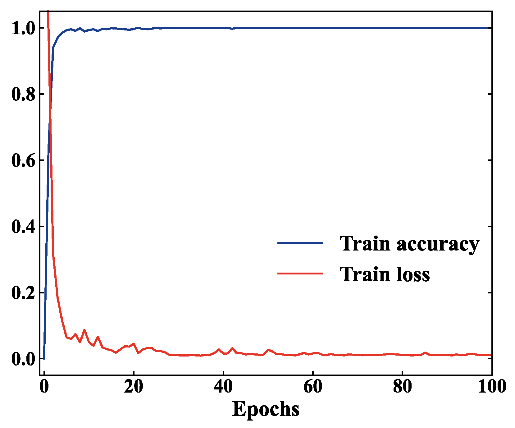
The training curves of HFDF-EffNetV2 are shown in Figure 8, where it can be observed that, after a few iterations, the training accuracy reached 100% and the training loss rapidly decreased to around 0.1. Although the loss curve fluctuated several times during the subsequent training, it ultimately converged steadily to 0.011. This indicates that the DAWCE loss function helped the model learn effective fault features, gradually reducing the error and causing it to converge towards optimization.

4.2.2. Comparison and Analysis of Model Diagnostic Performance

Table 5. Comparison of different models’ diagnostic performance in Case 1.

Model	Accuracy/%	P/%	R/%	F1/%	Parameters/M	Time/ms
EfficientNetV2-S	100 ± 0.00	100 ± 0.00	100 ± 0.00	100 ± 0.00	20.10	28.73 ± 0.84
ResNet-18	99.71 ± 0.00	99.71 ± 0.00	99.71 ± 0.00	99.71 ± 0.00	11.18	17.53 ± 0.32
RepViT	99.83 ± 0.14	99.83 ± 0.14	99.83 ± 0.14	99.83 ± 0.14	4.72	22.69 ± 0.39
SqueezeNet	99.23 ± 0.12	99.23 ± 0.11	99.23 ± 0.12	99.23 ± 0.11	0.73	24.40 ± 0.43
MPNet	99.63 ± 0.07	99.63 ± 0.07	99.63 ± 0.07	99.63 ± 0.07	2.50	21.45 ± 0.58
MobileNetV3	98.40 ± 0.25	98.40 ± 0.24	98.40 ± 0.24	98.40 ± 0.24	3.91	19.34 ± 0.31
HFDF-EffNetV2 (Ours)	100 ± 0.00	100 ± 0.00	100 ± 0.00	100 ± 0.00	1.85	18.67 ± 0.31

presents the experimental results for the weight and diagnostic evaluation metrics of different models. The proposed model and EfficientNetV2-S both reached 100% accuracy, P, R, and F1, making them the best diagnostic performers among all compared models. Moreover, with the same optimal diagnostic performance as EfficientNetV2-S, the proposed model was significantly lighter-weight, reducing the number of parameters and the diagnostic time by 91% and 35%, respectively. While the proposed model’s parameters and diagnostic time are not optimal, the model’s performance was good. For example, the model has slightly more parameters than SqueezeNet (by 1.12 million (M)), but the time is 23% shorter. The time is slightly longer than that of ResNet-18 (by 1.14 milliseconds (ms)), but the number of parameters is significantly lower, by 83%. In summary, HFDF-EffNetV2 achieved optimal diagnostic performance while still maintaining an excellent lightweight profile, an outcome that validates the effectiveness and advancement of the model design.

4.2.3. Model Comparison Experiments and Analysis Under Noise Interference

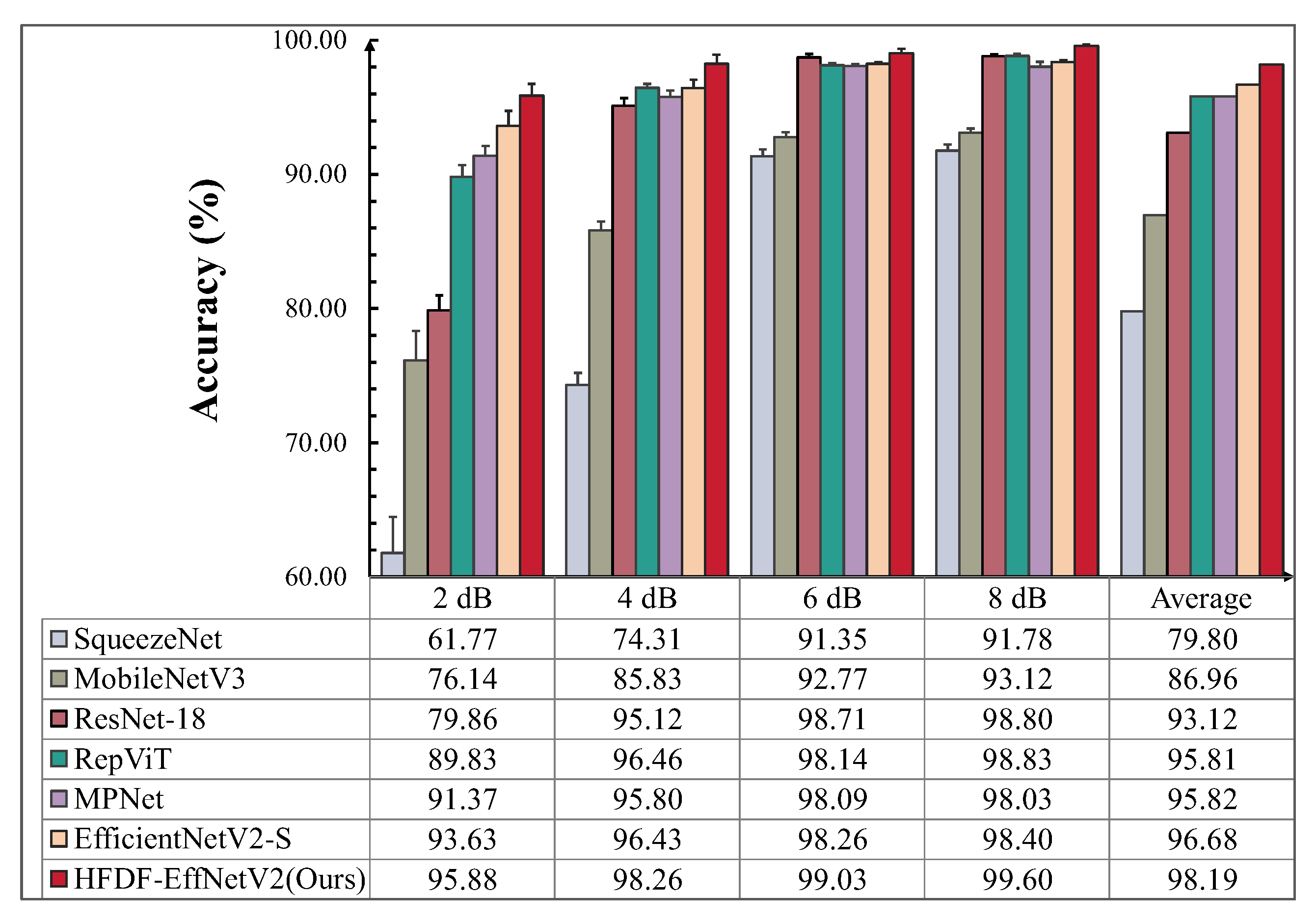
According to Equation (13), GWN with varying SNRs was added to the test set signals to evaluate the robustness of the model to noise. The experimental results are shown in Figure 9.

After noise was added, the proposed model achieved an average accuracy of 98.19%, which is 18.39%, 11.23%, 5.07%, 2.38%, 2.37%, and 1.51% higher than the six comparison models. Furthermore, the proposed model performed optimally under the same noise intensity compared to the other models. As the noise intensity increased, the accuracy decreased by only 3.72%, which is 1.05% less than the decrease observed in the next-best model, EfficientNetV2-S. At 2 dB, the accuracies of SqueezeNet and MobileNetV3 dropped dramatically, to 61.77% and 76.14%, respectively; these values were 34.11% and 19.74% lower than that of the proposed model, showing a significant gap. ResNet-18, RepViT, and MPNet performed well at 6 dB and 8 dB but poorly at 2 dB, with their accuracies lower than that of the proposed model by 16.02%, 6.05%, and 4.51%, respectively. EfficientNetV2-S, which had the greatest number of parameters, performs=ed well, though its accuracy was slightly lower than that of the proposed model, by 2.25%, at 2 dB. The results show that there is a relationship between the model’s noise resistance and its parameter count. More importantly, optimizing the model architecture to enhance its feature extraction capabilities can significantly improve the robustness of the model under noise interference.

4.2.4. Visualization and Analysis Under Noise Interference

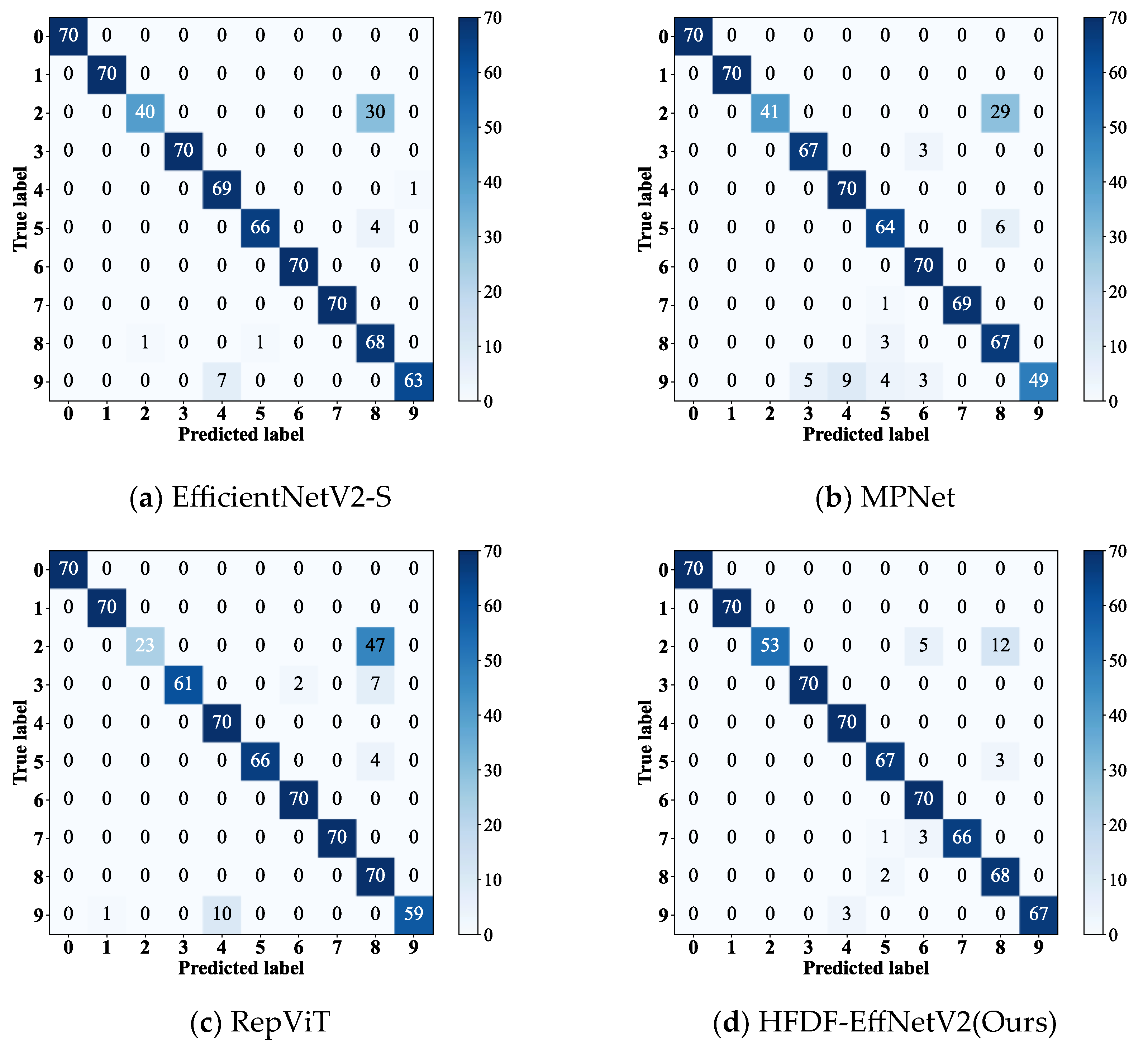
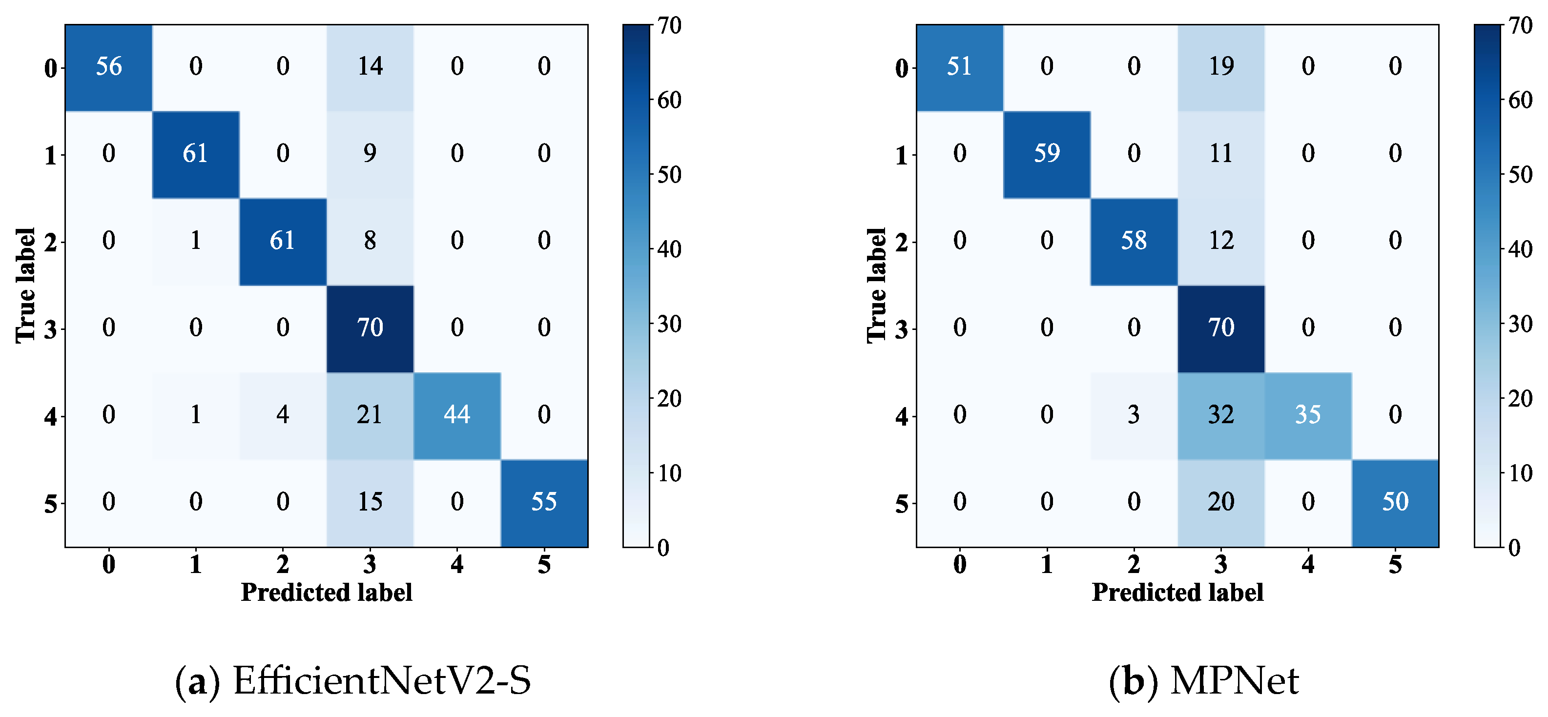
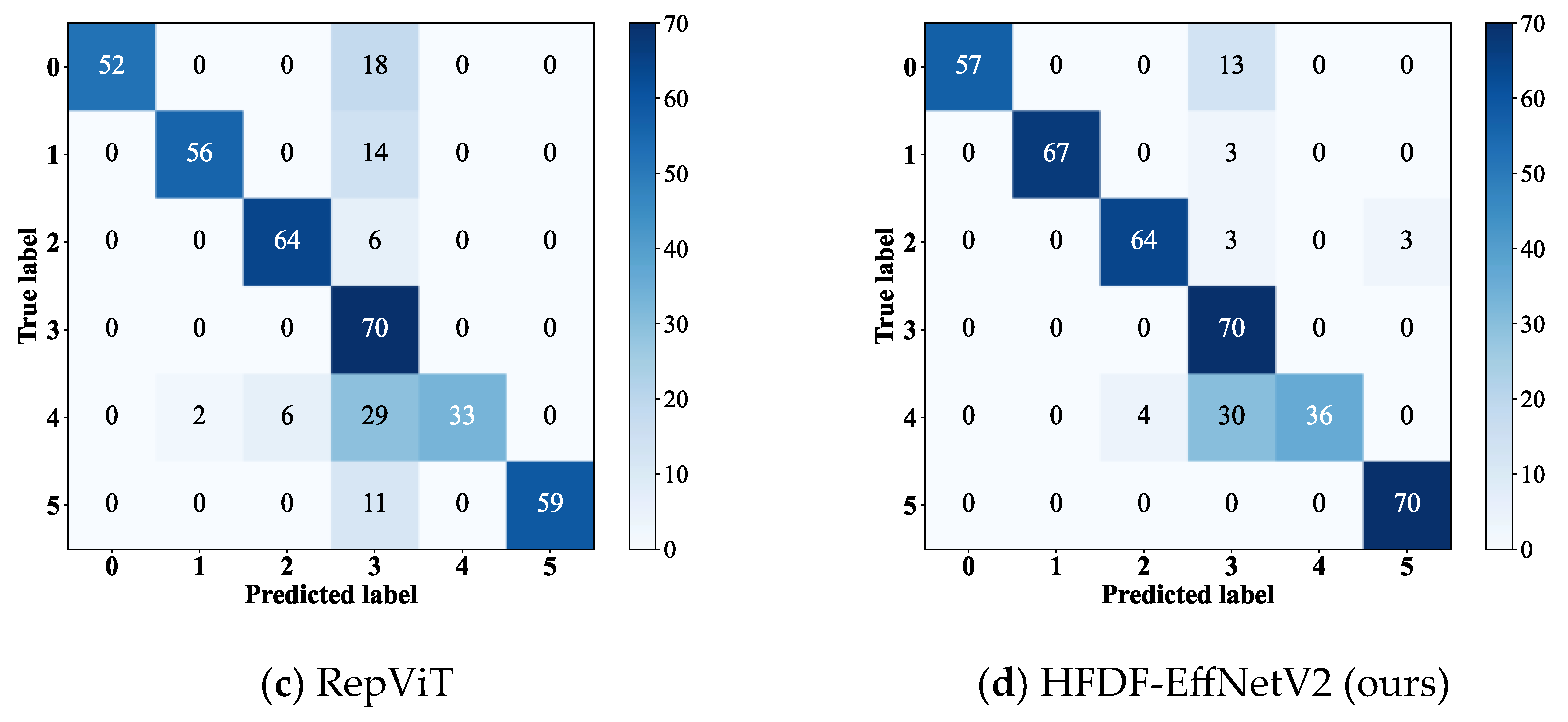
To compare the diagnostic performance of the models under noise interference for different fault types with a simulated SNR of 2 dB, this experiment visualized the confusion matrices of EfficientNetV2-S, RepViT, and MPNet, which performed better in the noise experiments, alongside HFDF-EffNetV2, as shown in Figure 10.

All models exhibited varying levels of misclassification in diagnosing fault label 2, with the number of misclassified samples for EfficientNetV2-S, RepViT, and MPNet being 30, 29, and 47, respectively, while the proposed model misclassified only 17 samples. Additionally, RepViT and MPNet exhibited poor diagnostic performance (P) for fault label 9, achieving only 70% and 84%, respectively. Although the performance of the proposed model was not optimal for all fault types, its diagnostic P reached 100% for fault labels 0, 1, 3, 4, and 6, and exceeded 94% for fault labels 5, 7, 8, and 9. The results show that HFDF-EffNetV2 significantly improves diagnostic P for samples with confusable fault types.

4.2.5. Comparative Experiments and Analysis with Small Sample Sizes

Due to the difficulty of obtaining large amounts of fault data in practical engineering applications, this experiment evaluated the diagnostic performance of HFDF-EffNetV2 with small sample sets by dividing the samples based on the total length of the sampled vibration signals and creating three datasets (A, B, and C) of different sizes. The number of training samples in datasets A, B, and C was 100, 200, and 300, respectively, while the number of test samples was fixed at 700.

The experimental results are shown in

Table 6. Comparison of experimental results for different models with different training-sample sizes in Case 1.

Model	Accuracy/%
	A/(Train10/Test70)	B/(Train20/Test70)	C/(Train30/Test70)	Average
EfficientNetV2-S	91.74 ± 1.14	97.74 ± 0.43	98.54 ± 0.25	96.01
ResNet-18	98.00 ± 0.42	98.74 ± 0.16	98.91 ± 0.15	98.55
RepViT	85.40 ± 1.32	94.63 ± 0.89	97.86 ± 0.45	92.63
SqueezeNet	81.97 ± 1.55	88.71 ± 0.82	92.71 ± 0.55	87.80
MPNet	92.00 ± 0.92	97.34 ± 0.48	98.57 ± 0.18	95.97
MobileNetV3	83.60 ± 1.5	93.86 ± 0.76	95.40 ± 0.44	90.95
HFDF-EffNetV2 (Ours)	98.09 ± 0.52	98.91 ± 0.17	99.09 ± 0.12	98.69

. ResNet-18 performed well, with an average accuracy of 98.55%, which is only 0.14% lower than that of the proposed model. EfficientNetV2-S, RepViT, and MPNet, which exhibited relatively good performance in the noise-interference experiments, showed instability when the training data were scarce, with average accuracies lower than that of the proposed model by 2.68%, 6.06%, and 2.72%, respectively. In contrast, the accuracies of SqueezeNet and MobileNetV3 were significantly lower than that of the proposed model, at 10.89% and 7.74%, respectively. On dataset A, the accuracies of all six comparison models decreased significantly, demonstrating that the models failed to extract effective fault features. Although the accuracy of the proposed model decreased compared to those of the other two training datasets on dataset A, it still remained above 98%, which was higher than those of the other six models by 6.35%, 0.09%, 12.69%, 16.12%, 6.09%, and 14.49%, respectively. The results indicate that HFDF-EffNetV2 is less influenced than the other models by the number of training samples and that its performance remains stable across varying sample sizes.

4.2.6. Visualization and Analysis with Small Sample Sizes

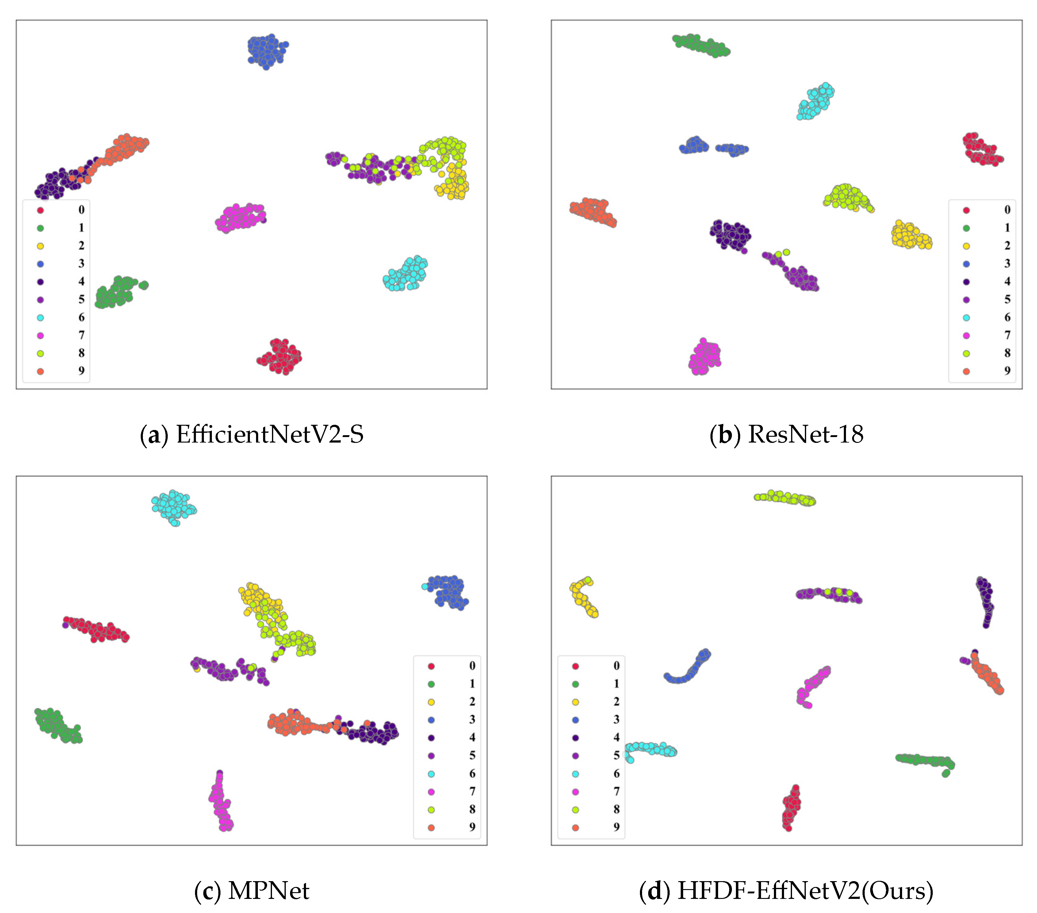
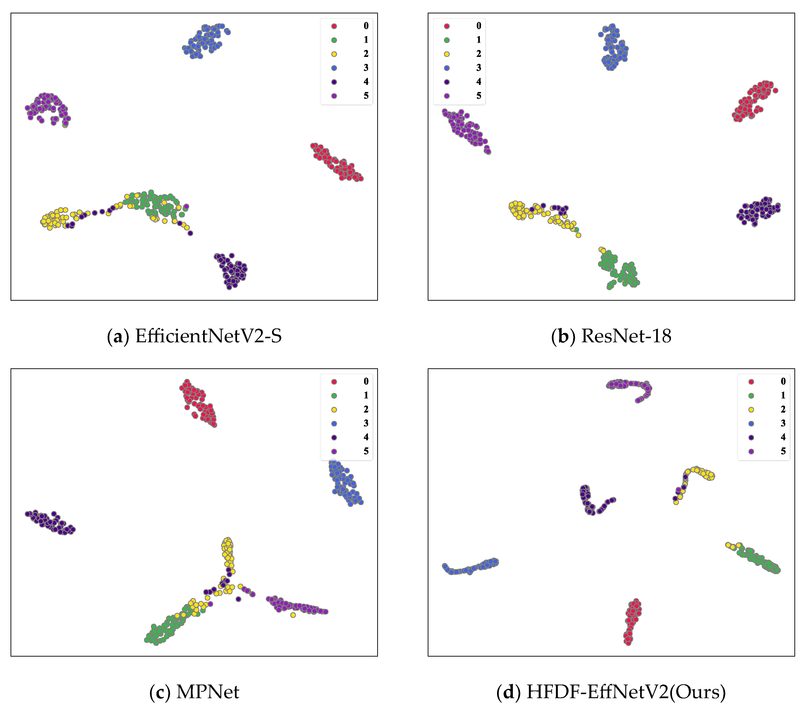
To further analyze the feature extraction performance of the model with small samples sizes, this experiment utilized the t-distributed stochastic neighbor embedding (t-SNE) technique to visualize the FD results of ResNet-18, EfficientNetV2-S, MPNet, and the proposed model on dataset A. This approach also allowed for the visualization of the clustering and separation of the extracted fault features after dimensionality reduction.

The visualization results are presented in Figure 11. The separation of fault features extracted by MPNet and EfficientNetV2-S for samples with fault labels 2, 4, 5, 8, and 9 was insufficiently clear, which could lead to misclassification of fault samples. In contrast, ResNet-18 demonstrated better clustering and separation of features than the previous two models, but the clustering centers for fault labels 4 and 5 were relatively close. Although the proposed model yielded a small number of misclassifications, the clustering and separation of fault features across different samples were satisfactory, highlighting its excellent feature extraction.

4.3. Case 2: Self-Constructed Bearing Experimental Dataset

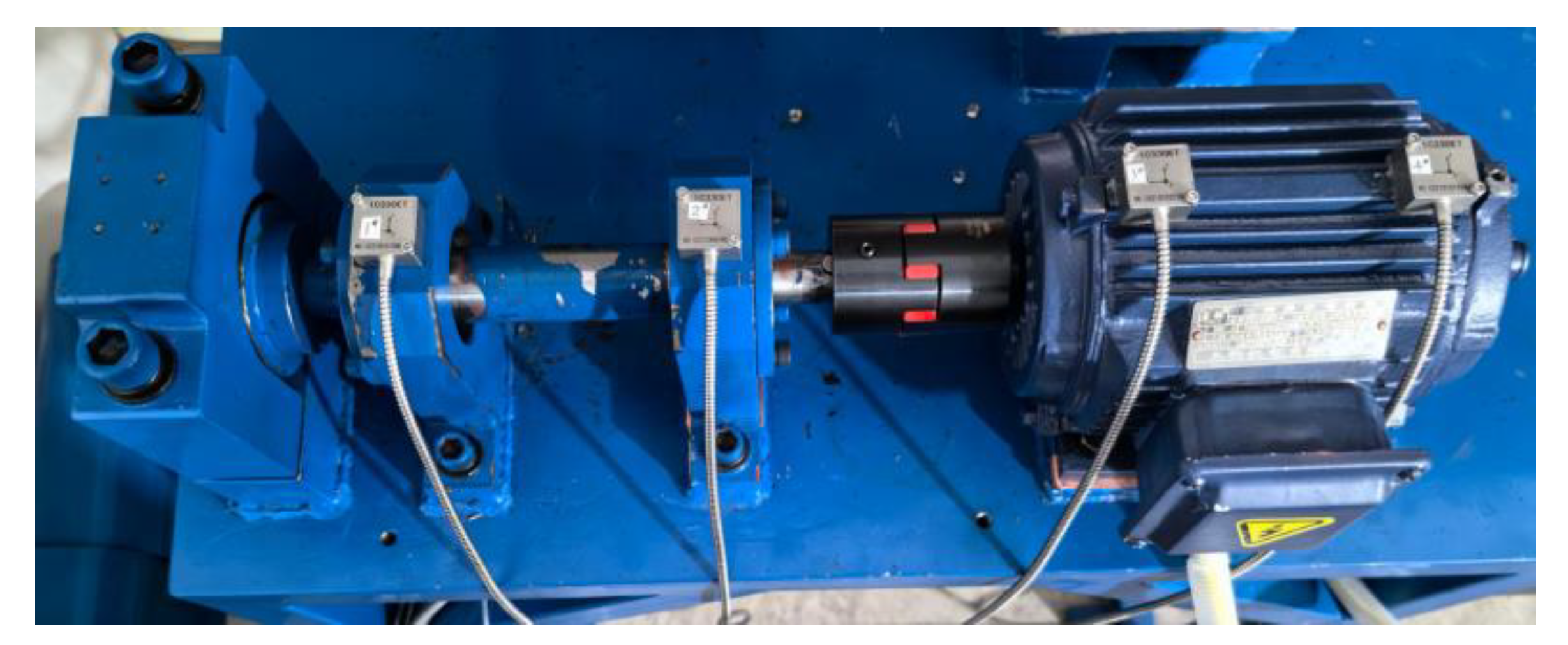
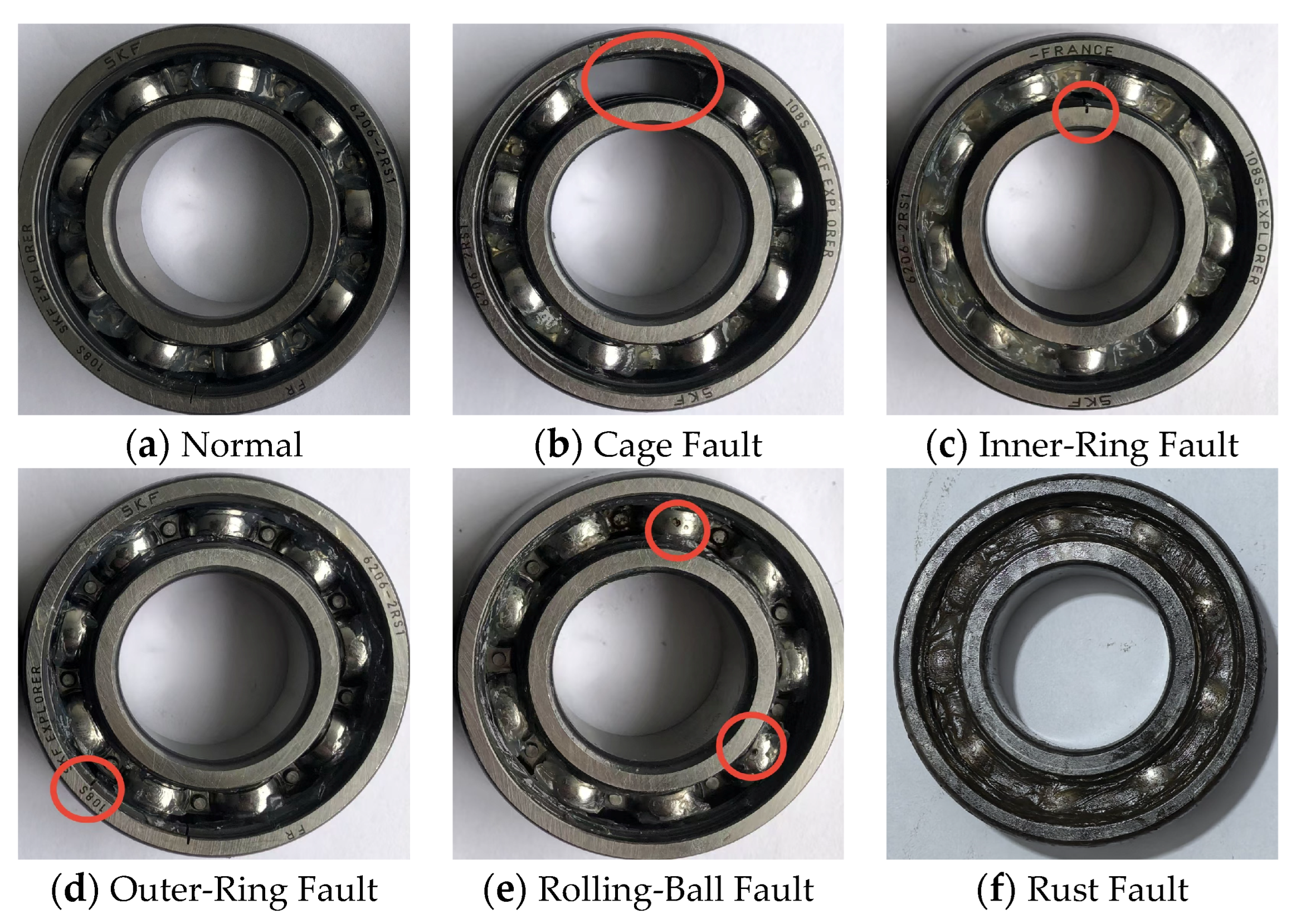
The self-constructed bearing experimental platform primarily consisted of 6206 rolling bearings, a 0.55 kW three-phase asynchronous motor, 1C330ET three-axis vibration and temperature integrated sensors, and couplings, as illustrated in Figure 12. 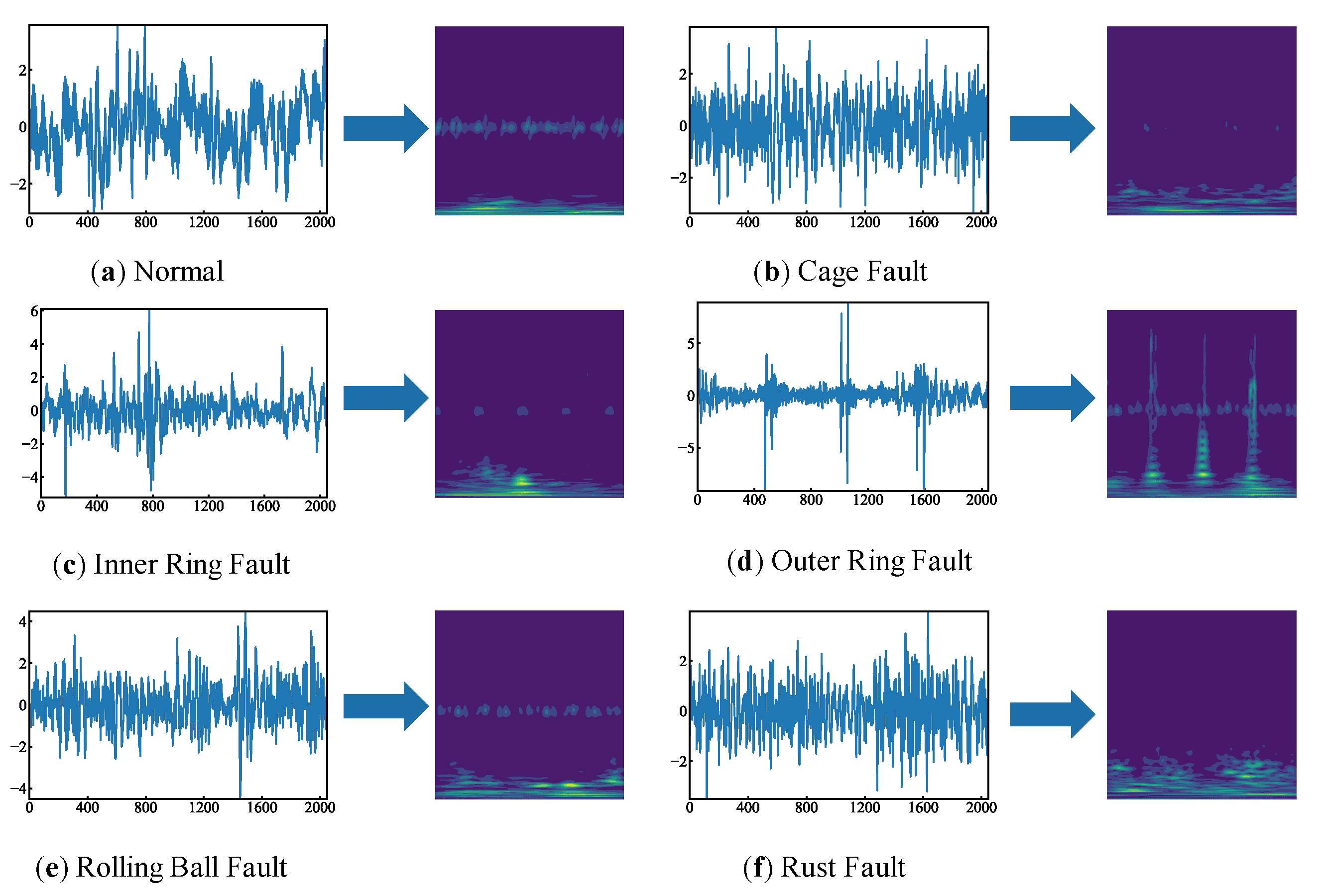Based on the common faults of rolling bearings in real industrial scenarios, cage faults, inner-ring faults, outer-ring faults, rolling-ball faults, and rust faults were simulated through wire cutting and saltwater immersion, as shown in Figure 13. At a speed of 800 r/min and a sampling frequency of 25.6 kHz, approximately 250,000 datapoints were collected for each fault type. To ensure that a single sample would contain fault information for at least one full revolution, the overlap window was set to 1024 and the sample length was set to 2048, as calculated using Equation (18). The time-frequency FM, obtained after standardizing the original signal and performing the CWT, is shown in Figure 14. The dataset samples were configured to remain the same as in Case 1, as presented in

Table 7. Self-Constructed bearing experimental dataset composition.

Fault Type	Fault Label	Train	Test
Normal	0	130	70
Cage Fault	1	130	70
Inner Ring Fault	2	130	70
Outer Ring Fault	3	130	70
Rolling Ball Fault	4	130	70
Rust Fault	5	130	70

.

4.3.1. Model Training

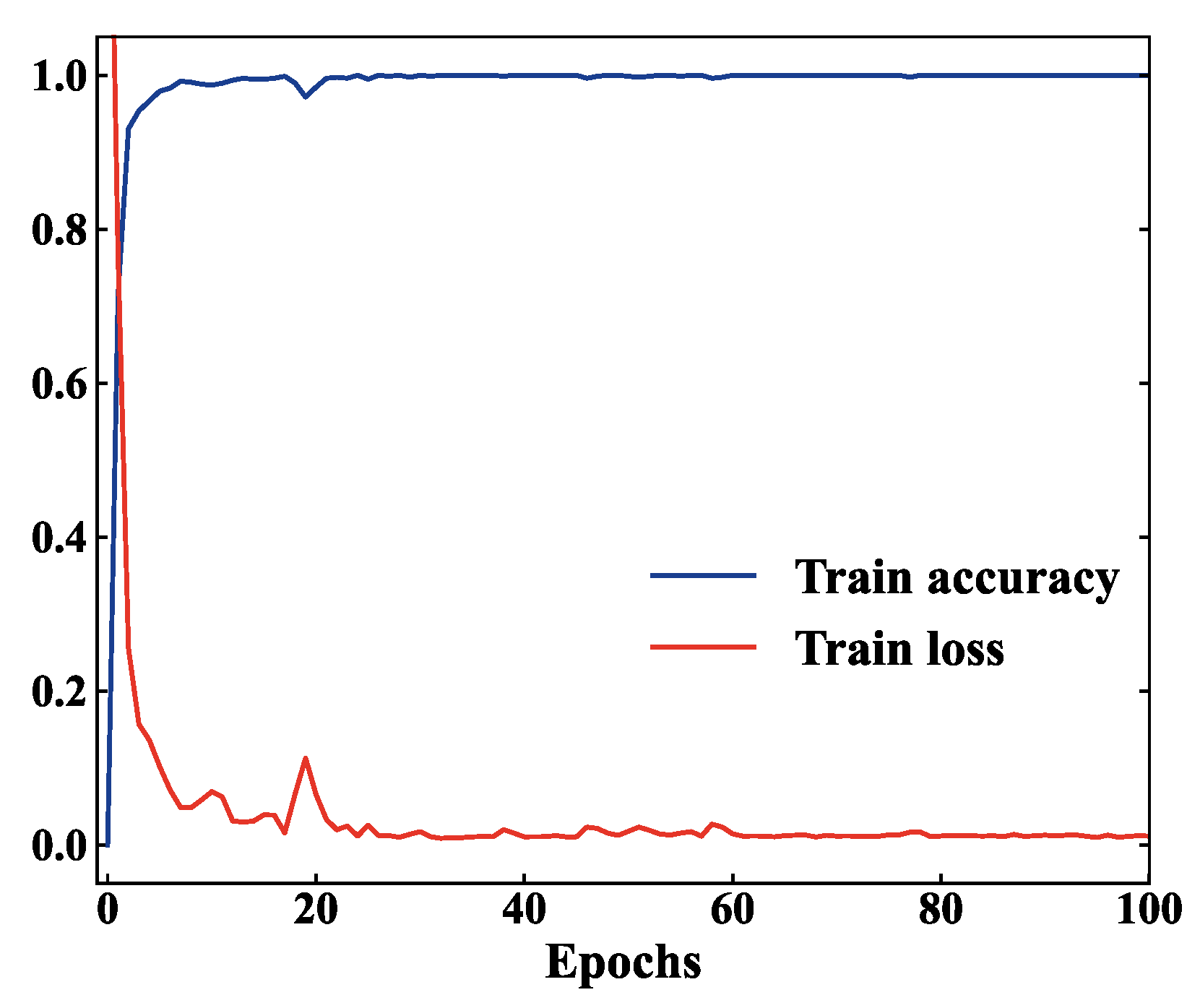
The training curves of HFDF-EffNetV2 are shown in Figure 15. The model started at 71.5% accuracy at the first iteration and then improved significantly, reaching 99.23% at the 7-th iteration and achieving 100% training accuracy after 100 iterations. Although there were significant fluctuations in the loss curves at the beginning of the model’s training, the loss values began to converge steadily to 0.01 after 20 iterations, indicating that the model’s weight updates tended to stabilize.

4.3.2. Model Diagnostic Performance Comparison and Analysis

Table 8. Comparison of different models’ diagnostic performances in Case 2.

Model	Accuracy/%	P/%	R/%	F1/%	Parameters/M	Time/ms
EfficientNetV2-S	99.67 ± 0.19	99.67 ± 0.19	99.67 ± 0.19	99.67 ± 0.19	20.10	28.05 ± 0.72
ResNet-18	99.95 ± 0.10	99.95 ± 0.09	99.95 ± 0.10	99.95 ± 0.10	11.18	17.52 ± 0.62
RepViT	99.14 ± 0.44	99.16 ± 0.44	99.14 ± 0.44	99.14 ± 0.44	4.72	23.17 ± 0.77
SqueezeNet	97.67 ± 0.18	97.67 ± 0.17	97.67 ± 0.18	97.67 ± 0.18	0.73	24.57 ± 0.40
MPNet	99.63 ± 0.24	99.63 ± 0.24	99.63 ± 0.24	99.63 ± 0.24	2.50	21.00 ± 0.51
MobileNetV3	95.95 ± 0.48	95.95 ± 0.48	95.95 ± 0.48	95.95 ± 0.48	3.91	18.69 ± 0.35
HFDF-EffNetV2 (Ours)	100 ± 0.00	100 ± 0.00	100 ± 0.00	100 ± 0.00	1.85	17.56 ± 0.41

presents the experimental results for the lightweight and diagnostic evaluation metrics of different models. The proposed model achieved 100% in four diagnostic evaluation metrics, accuracy, P, R, and F1, demonstrating the best performance among all the compared models. Although the proposed model was not optimal in terms of parameters and diagnostic time, it improved all of the diagnostic evaluation metrics by 2.33% and reduced the time by 29% compared to the best small model of SqueezeNet. Additionally, there was only a 0.04 ms time difference between the proposed model and ResNet-18, but the number of parameters was only 17% of the number in ResNet-18.

4.3.3. Model-Comparison Experiments and Analysis Under Noise Interference

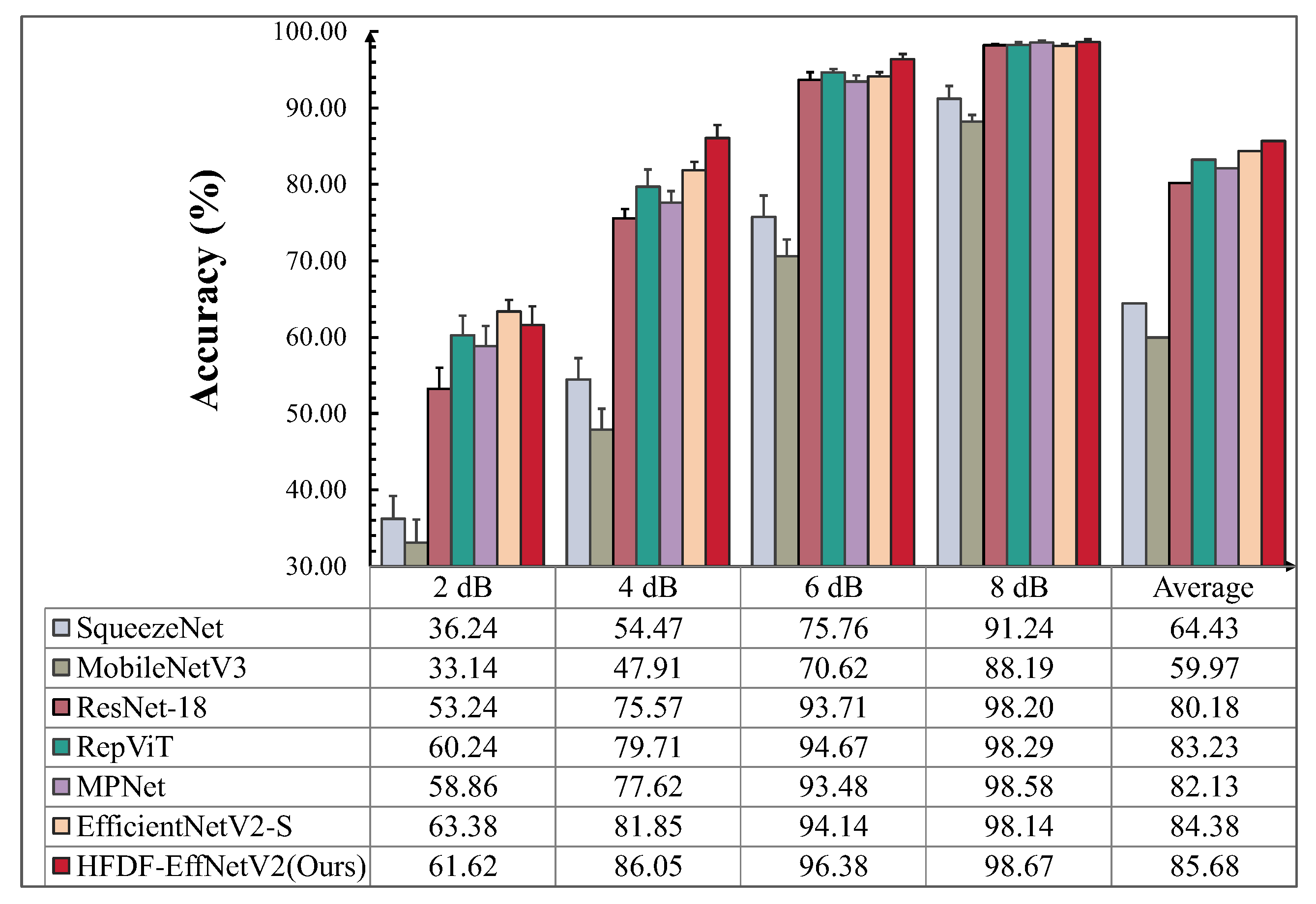
Consistent with the noise-interference experiment in Case 1, GWN with different SNRs was added to the test set signals. The experimental results are shown in Figure 16.

After noise was added, the proposed model still maintained the highest average accuracy, surpassing the other six models by 25.71%, 21.25%, 5.5%, 3.55%, 2.45%, and 1.3%, respectively. As the level of noise interference increased, the accuracies of all models decreased significantly. At 4 dB, SqueezeNet and MobileNetV3 exhibited the largest accuracy gaps with the proposed model, at 38.14% and 31.58%, respectively. Comparatively, ResNet-18, MPNet, and RepViT exhibited slightly better noise resistance than SqueezeNet and MobileNetV3, with deficits of 10.48%, 8.43%, and 6.34% relative to the proposed model, respectively. Although the accuracy of the proposed model was suboptimal at 2 dB, 1.76% lower than the accuracy of EfficientNetV2-S, it showed a notable improvement at 4 dB, surpassing that of EfficientNetV2-S by 4.2%. In summary, these findings suggest that models with larger parameter counts are more resilient to severe noise interference but that an optimal design can also improve the model’s robustness to noise.

4.3.4. Visualization and Analysis Under Noise Interference

In order to show the diagnostic results of the models for different fault types with a simulated SNR of 4 dB, this experiment visualized the confusion matrices of EfficientNetV2-S, RepViT, MPNet, and the proposed model.

The visualization results are shown in Figure 17, where the diagnostic P of the proposed model is 100% for fault labels 3 and 5 and 89% for fault labels 0, 1, and 2. Compared to EfficientNetV2-S, MPNet, and RepViT, which correctly diagnosed all samples with fault label 3, the diagnostic P for fault label 5 differed significantly from that of the proposed model, with differences of 22%, 28%, and 16%, respectively. In addition, all models performed poorly in the diagnosis of fault label 4. Despite the proposed model having eight more misclassified samples compared to the model with the fewest (EfficientNetV2-S), HFDF-EffNetV2 performed better overall. The result demonstrates that the HFDF strategy effectively mitigates the issue of the lightweight model falling into local overfitting.

4.3.5. Comparative Experiments and Analysis Under Small Samples Conditions

Consistent with the experimental setup in Case 1, this experiment was conducted with three different dataset sizes (A, B, and C), where the numbers of training samples were 100, 200, and 300, respectively, and the number of test set samples was fixed at 700.

The experimental results are presented in

Table 9. Comparison of experimental results for different models with different sizes of training samples in Case 2.

Model	Accuracy/%
	A/(Train10/Test70)	B/(Train20/Test70)	C/(Train30/Test70)	Average
EfficientNetV2-S	91.29 ± 0.78	96.58 ± 0.89	96.39 ± 0.84	94.75
ResNet-18	95.71 ± 0.66	97.52 ± 0.61	97.81 ± 0.28	97.01
RepViT	88.17 ± 1.10	92.28 ± 0.96	94.19 ± 0.77	91.55
SqueezeNet	80.57 ± 1.61	92.24 ± 0.58	92.87 ± 0.72	88.56
MPNet	90.81 ± 0.76	95.86 ± 0.52	96.09 ± 0.36	94.25
MobileNetV3	78.04 ± 1.35	90.59 ± 0.76	91.82 ± 0.62	86.82
HFDF-EffNetV2 (Ours)	95.88 ± 0.91	98.19 ± 0.42	98.47 ± 0.41	97.51

and demonstrate that the proposed model achieves optimal diagnostic accuracy across different datasets. ResNet-18 performed excellently, with an average accuracy only 0.5% lower than that of the proposed model. EfficientNetV2-S and MPNet performed well on datasets B and C, but exhibited poor performance on dataset A, resulting in average accuracies 2.76% and 3.26% lower than those of the proposed model, respectively. RepViT, SqueezeNet, and MobileNetV3 exhibited poor performance overall, with average accuracies 5.96%, 8.95%, and 10.69% lower than those of the proposed model, respectively. As the number of training samples decreased, the accuracy of the proposed model decreased slightly by 2.59%, for a value 0.49% higher than that of ResNet18, the model with the smallest decrease. However, it remained more stable compared to the other five models, which showed decreases of 5.1%, 6.02%, 12.3%, 5.28%, and 13.78%. The results indicate that HFDF-EffNetV2 improves the ability to perceive the relationships between different channels in the input FM and that it continues to capture key information from important channels even with small sample sizes.

4.3.6. Visualization and Analysis with Small Sample Sizes

In this experiment, the t-SNE technique was employed to visualize the FD results of ResNet-18, EfficientNetV2-S, MPNet, and the proposed model in a small-sample experiment using dataset A.

The visualization results are shown in Figure 18. While MPNet and EfficientNetV2-S were effective in clustering and separating the features of fault labels 0, 3, 4, and 5; the clustering and separation of the features for fault labels 1 and 2 were not fully formed, indicating insufficient perception of the differences between fault types, which could result in the misclassification of fault samples. Compared to ResNet-18, the proposed model exhibited more distinct separation for fault labels 1 and 2, with misclassification occurring for only a few samples. The results indicate that HFDF-EffNetV2 effectively establishes a clear classification boundary, demonstrating stronger feature clustering and discriminative ability.

4.4. Analysis of Experimental Results in Two Cases

The results of the comparison experiments conducted demonstrate that the model architecture design significantly influences diagnostic performance. The lightweight architectures of SqueezeNet and MobileNetV3 constrain their capacity to capture salient local fault features, leading to poor robustness. ResNet-18 employs a simple architecture that achieves the fastest diagnostic time, but its limited depth compromises robustness to noise. While the multi-branch architectures of RepViT and MPNet enable effective capture of fault features with enhanced robustness to noise, such architectures inevitably reduce diagnostic speed. EfficientNetV2-S possesses a large model capacity, enabling it to capture deeper fault information and exhibit strong robustness to noise. However, this complexity also makes it sensitive to the size of the training dataset and results in the slowest diagnostic performance. In contrast, although HFDF-EffNetV2 is slightly slower than ResNet-18 and has a marginally higher parameters than SqueezeNet, it utilizes a lightweight multi-branch structure combined with a fine-grained feature extraction and decision fusion approach, significantly enhancing diagnostic accuracy.

4.5. Ablation Experiment and Analysis

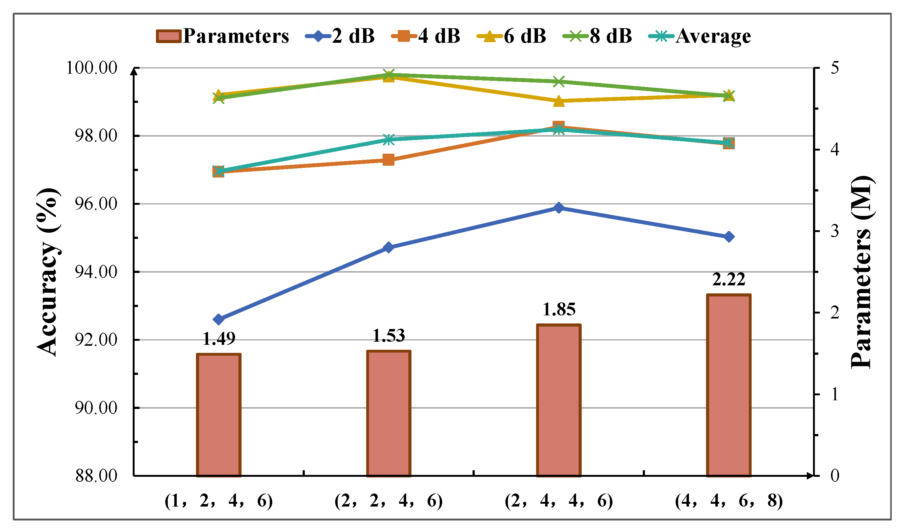
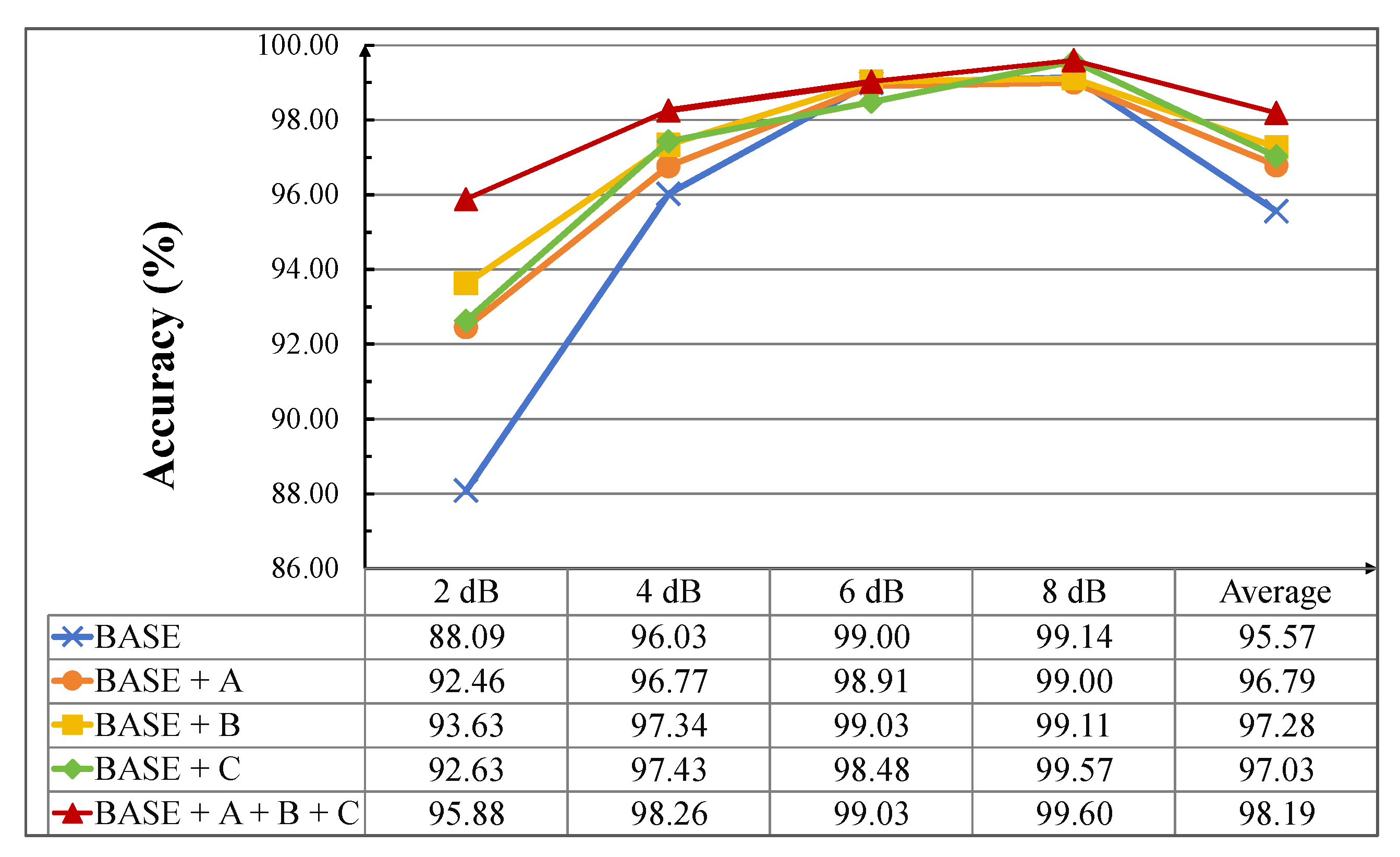
Since the construction of HFDF-EffNetV2 involved multiple methods, ablation experiments were conducted on the CWRU bearing dataset to more intuitively visualize the impact of each method on the model’s diagnostic performance. As shown in

Table 10. The number of parameters and diagnostic time for ablation models.

Model	BASE	BASE + A	BASE + B	BASE + C	BASE + A + B + C
Parameters/M	2.31	2.37	1.67	2.44	1.85
Time/ms	15.24 ± 0.29	17.43 ± 0.31	17.18 ± 0.30	15.80 ± 0.29	18.67 ± 0.31

, The BASE refers to the model constructed based on EfficientNetV2-S. The BASE + A and BASE + B models incorporated the methods of Fused-MBPyConv and BSMBConv-MLCA, respectively. The BASE + C model employed the HFDF strategy, and the BASE + A + B + C represents the proposed model.

The experimental results are presented in Figure 19 and demonstrate that the application of the three improvement methods significantly enhanced the diagnostic accuracies under strong noise interference. At 2 dB, the accuracy of the BASE + A + B + C was improved by 7.79% compared to the BASE. At 4 dB, BASE + C with the HFDF strategy applied showed improvements of 1.4%, 0.66%, and 0.09% compared to BASE, BASE + A, and BASE + B, respectively. At 6 dB and 8 dB, all models showed improved performance, making the relative improvement of the three enhanced methods compared to BASE non-significant. However, the average accuracies of the three enhanced methods were increased by 1.22%, 1.71%, and 1.46%, respectively, compared to BASE. Overall, all three improvement methods were effective in enhancing the model’s performance under noise interference, with the most significant contributions coming from the application of BSMBConv-MLCA.

5. Conclusions

This study addresses the challenge of achieving real-time and high-accuracy FD on platforms with limited computational resources by proposing a lightweight model called HFDF-EffNetV2.

In noise-interference experiments on the CWRU bearing dataset and a self-constructed bearing dataset, the average accuracy of the proposed model increased by 1.51%, 5.07%, 2.38%, 18.39%, 2.37%, and 11.23% and by 1.3%, 5.5%, 2.45%, 21.25%, 3.55%, and 25.71%, compared to EfficientNetV2-S, ResNet-18, RepViT, SqueezeNet, MPNet, and MobileNetV3, respectively. With small sample sizes, the proposed model outperformed these six models in average accuracy by 2.68%, 0.14%, 6.06%, 10.89%, 2.72%, and 7.74% and by 2.76%, 0.5%, 5.96%, 8.95%, 3.26%, and 10.69%, respectively. These results show that the Fused-MBPyConv and BSMBConv-MLCA proposed in this study achieved deeply coupled resolution of cross-scale fault features while maintaining light weight through feature fusion via staged channel-compression transformations. The HFDF strategy enables global integrated FD with cross-level fault feature relationships through multi-stage information fusion.

Although the proposed model achieved excellent diagnostic results in preliminary experiments and has 1.85 M parameters and faster diagnosis time compared with other lightweight models, which verifies its potential for real-time and highly accurate deployment on edge devices, the model may still be limited by the hardware configurations on resource-constrained edge devices. Indeed, in actual equipment operation, rolling bearings may experience fault types never before encountered by the models. Therefore, future research will combine signal processing with threshold-independent open-set identification strategies to enhance the diagnostic capabilities of the proposed model for unknown faults and evaluate its performance across different edge devices and real-world environments.