A Multi-Input Multi-Output Considering Correlation and Hysteresis Prediction Method for Gravity Dam Displacement with Interpretative Functions

Abstract

The displacement of a concrete gravity dam is a direct manifestation of its deformation. It provides an intuitive reflection of the dam’s overall operational behavior and serves as a key indicator of the dam’s safe operating condition. In this paper, we propose a factor set that considers the hysteresis effects of temperature on displacement and ranks the importance of the features to select the optimal factor sets at different measurement points by the ReliefF method. Then, we realize the simultaneous prediction of the displacements at multiple measurement points by the multi-input multi-output least-squares support vector machine with particle swarm optimization (MIMO-PSO-LSSVM). The case study demonstrates that this method effectively enhances the accuracy and efficiency of gravity dam displacement prediction, thereby providing a novel reference for dam safety monitoring and health service diagnosis.

1. Introduction

As a major component of water storage systems, dams play a significant role in water supply, flood control, power generation, and irrigation. However, the potential risk of dam failure increases due to a variety of reasons, including hydrology, geology, construction quality, material aging, and operational management. Additionally, in recent years, changes in extreme climate have adversely affected the dynamic behavior of dam structures and their interactions, thereby increasing the potential risk of dam failure [1]. In the event of a dam failure, the downstream area will be severely impacted. Therefore, the work of dam safety monitoring is particularly prominent and important [2,3]. Displacement is a critical indicator of dam safety monitoring, as it can effectively reflect the degree of operational safety and structural integrity of dams [4,5]. Analyzing measured data from dams and establishing displacement prediction models based on these data has become one of the primary focuses of dam health monitoring.

Currently, the analysis and prediction of dam monitoring data principally utilize statistical, deterministic, or hybrid models to predict and monitor the dam behavior. Among these, statistical models based on multiple linear regression and its advanced forms have been extensively employed in dam health monitoring modeling to ascertain the reasonable behavior of the dam structure by comparing the observed structural response with the predicted values obtained from the mathematical model [6,7]. In the field of statistical modeling, the regression models used include multiple linear regression (MLR) [8,9], stepwise regression (SR) [10], regression models based on principal component analysis [11], partial least squares regression [12], etc. However, concrete dams are complex dynamic systems whose deformation values comprehensively reflect the dam’s operating conditions. Due to the existence of a multitude of structural forms and the presence of complex external environmental factors, dam deformation is characterized by non-linearity, uncertainty, and time-variability. Traditional statistical models are essentially linear regression methods, which are unsuitable for modeling high-dimensional relationships. This limitation results in a decline in the predictive accuracy and robustness of statistical models. Recently, with the advancement of artificial intelligence, researchers have progressively combined machine learning models with dam deformation prediction models [13]. Owing to its capacity to handle nonlinear problems, prediction models formulated with machine learning algorithms exhibit substantial enhancements in terms of predictive accuracy and robustness. Machine learning methods, including but not limited to Relevance Vector Machines (RVMs) [14], Radial Basis Function Networks (RBFNs) [15], Support Vector Machines (SVMs) [16], Extreme Learning Machines (ELMs) [17], Stacked Gated Recurrent Unit Neural Networks (GRUs) [18], and Long and Short-Term Memory Neural Networks (LSTMs) [19], have been employed to address issues in dam health monitoring.

Recent studies have indicated that artificial neural networks and SVM represent two machine learning algorithms that are utilized extensively in the context of dam safety monitoring. In comparison with artificial neural networks, SVM has clear advantages in solving problems involving small samples and high-dimensional and nonlinear problems due to its robust theoretical foundation [20,21]. Least squares support vector machine (LSSVM) [22,23] represents an enhanced SVM, whereby the inequality constraints are converted into equality constraints through the utilization of the quadratic programming method. The sum of squares of the loss function errors is then employed as the empirical loss of the training sample set, and the quadratic programming problems are transformed into linear equations. The prediction accuracy of LSSVM is contingent upon the reasonable setting of hyperparameters. However, the primary challenges that must be addressed include the avoidance of overfitting, the selection of appropriate regularization constants, and the choice of the optimal kernel function and related parameters. Optimization algorithms can be utilized to facilitate the adaptive search for the optimal hyperparameters of the model, thereby enabling the construction of combined prediction models that exhibit superior performance. Examples of such algorithms include Genetic Algorithm (GA) [24], Fruit Fly Optimization Algorithm (FOA) [25], White Shark Optimizer (WSO) [26], Grasshopper Optimization Algorithm (GOA) [27], and Particle Swarm Optimization Algorithm (PSO) [28]. Among them, the PSO, due to its simplicity and ease of understanding, has been widely applied in the field of engineering structural health monitoring. Numerous research achievements have successfully integrated PSO, GA, FOA, and other intelligent optimization algorithms with various models for predictive analysis [29,30]. The hyperparameters of the LSSVM are adjusted through PSO. The optimized PSO-LSSVM model demonstrates a high degree of accuracy in prediction; thus, it is widely applied in dam displacement prediction [31,32].

Dam deformation can be influenced by various environmental factors, including hydraulic pressure and temperature. Hydraulic-Seasonal-Time (HST) and Hydraulic-Temperature-Time (HTT) models are fundamental statistical models for selecting input variables to predict dam displacement [33,34]. Building on the HTT model, Kang et al. [35,36] proposed a long-term air temperature-based Hydraulic-Air temperature-Time (HT_AT) model to achieve more accurate predictions of dam behavior. However, the hysteresis effect between dam deformation and changes in environmental factors is often observed [37,38,39]. Therefore, the hysteresis effect of dam deformation on temperature must be taken into account in the analysis process. Wang et al. [40] proposed the Hydraulic-Hysteresis-Seasonal-Time (HHST) model, which considered the hysteresis effect of environmental factors. Ren et al. [41] introduced a hysteresis quantification algorithm to estimate the hysteresis days of environmental factors affecting deformation.

In order to enhance the performance and prediction accuracy of the model, it is necessary to utilize feature selection for variable screening to select appropriate input variables for dam health monitoring by comparing the magnitude of importance of different variables. Huang et al. [42] utilized the Principal Component Analysis (PCA) method to identify the primary factors, thereby further optimizing the model. Dai et al. [43] employed the Random Forest (RF) algorithm to predict the displacements and analyze the significance of the variables on the displacements. Xu et al. [44] applied the mRMR algorithm and the Lasso algorithm for feature selection to obtain the optimal factor sets. Kononenko et al. [45] utilized the ReliefF algorithm, an extension of the Relief algorithm, as a feature weighting method. The ReliefF algorithm assigns different weights to features based on the relevance of the different features and categories and then removes the features whose weights are less than a certain value. It has been demonstrated that the ReliefF algorithm is characterized by simplicity in operation, high efficiency in execution, the capacity to select features exhibiting strong relevance to the category, and the ability to reduce the complexity of subsequent algorithms by decreasing the original feature vectors from high dimensions to low dimensions [46]. This renders it a reliable feature selection method.

In the past, the majority of prediction methods have been modeled for a single measurement point, which disregards the potential spatial correlation between different displacement measurement sites [47]. Essentially, these methods belong to the multiple-input-single-output model, which can only approximate the mapping from a multivariate input space to a univariate output space. Advancements in monitoring technology have led to an increase in the scale of monitoring sensors and the amount of data collected on dam behavior. Consequently, with the objective of enhancing prediction efficiency, displacement-based dam health monitoring is transitioning from single-point independent modeling to multi-point synchronous modeling [48]. Chen et al. [49] proposed a method for spatio-temporal clustering and health diagnosis of ultra-high concrete arch dams based on multi-point displacement data. Wang et al. [50] proposed a spatial association-coupled double objective SVM prediction model for diagnosing the displacement behavior of high arch dams.

Recently, a new data modeling technique based on multiple linear regression, termed multi-target regression [51], has been proposed. This technique is capable of multiple-input multiple-output (MIMO) mapping, with the objective of predicting multiple targets simultaneously and sharing relevant information across targets. In the event of there being a correlation between the targets, each predictor variable can benefit from the others, thus improving the prediction accuracy of the model [52]. Multi-target regression algorithms have been extensively utilized in a range of multi-output prediction problems. Chen et al. [53] proposed a mathematical approach, termed Multiple Correlation-based Structural Stack Test (MCSST), for the synchronous prediction of multiple displacement responses in arch dams. This approach integrates a target stacking strategy with a correlation-based feature selection framework. Li et al. [54] utilized an integrated Bayesian approach and multi-output SVM to analyze the displacement of rocky slopes. Ren et al. [55] proposed a MIMO machine learning paradigm based on SVM for synchronous modeling and prediction of multi-point displacements from different blocks of dams. Considering the advantages of LSSVM in solving small sample, high-dimensional, and nonlinear problems, this paper elects to integrate the multi-target regression algorithm with LSSVM to formulate a model for dam displacement prediction. For ease of viewing, the abbreviations are summarized in

Table 1. List of abbreviations.

Abbreviations	The Full Designation	Abbreviations	The Full Designation
MLR	Multiple Linear Regression	HTT	Hydraulic-Temperature-Time
SR	Stepwise Regression	HTAT	Hydraulic-Air temperature-Time
RBFN	Radial Basis Function Network	HHST	Hydraulic-Hysteresis-Seasonal-Time
RVM	Relevance Vector Machine	PCA	Principal Component Analysis
SVM	Support Vector Machine	HTHT	Hydraulic-TemperatureHysteresis-Time
ELM	Extreme Learning Machine	RF	Random Forest
GRU	Gated Recurrent Unit Neural Network	MIMO	Multiple-Input Multiple-Output
LSTM	Long and Short-Term Memory Neural Network	MCSST	Multiple Correlation-based Structural Stack Test
LSSVM	Least Squares Support Vector Machine	BPNN	Back Propagation Neural Network
GA	Genetic Algorithm	PSO-LSSVM	LSSVM optimized by PSO
FOA	Fruit Fly Optimization Algorithm	MIMO-PSO-LSSVM	Multi-input Multi-output Least Squares Support Vector Machine with Particle Swarm Optimization
WSO	White Shark Optimizer	RMSE	Root Mean Square Error
GOA	Grasshopper Optimization Algorithm	MAE	Mean Absolute Error
PSO	Particle Swarm Optimization Algorithm	R2	The Coefficient of Determination
HST	Hydraulic-Seasonal-Time

.

In summary, this paper proposes a factor set that considers the hysteresis effects of temperature on the displacement of gravity dams. Feature selection is carried out by the ReliefF, which analyses the importance of the feature factors on the displacements of different measurement points and screens the main factors in the factor set to obtain a unified factor set for measurement points in the same area. After considering the spatial correlation between the measurement points, a multi-output prediction model is established using an LSSVM optimized by PSO. This approach achieves the synchronous prediction of displacements at multiple measurement points of gravity dams, thus demonstrating the efficacy of the proposed methodology. The main contributions of this study are as follows.

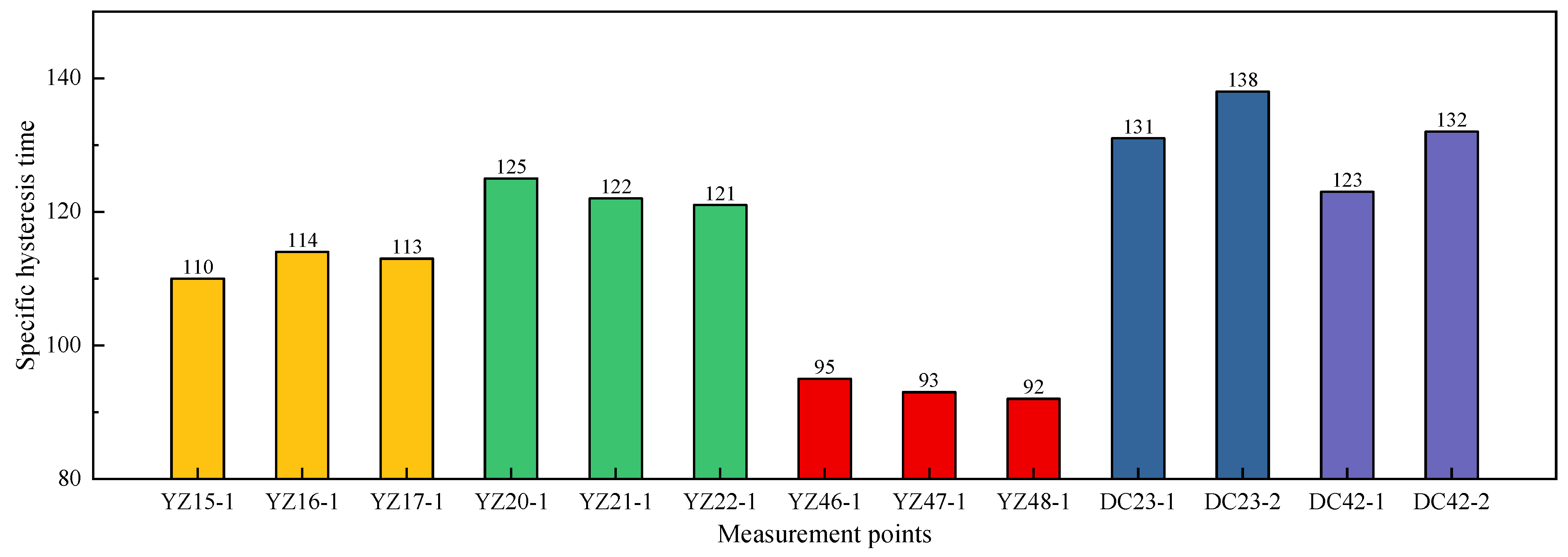
• A new factor set that considers the hysteresis effects of temperature on displacement is proposed by calculating the specific hysteresis times with the sliding match method and the cosine similarity calculation method. This factor set considers the hysteresis effects of temperature on displacements, emphasizing that the hysteresis effects of environmental factors on displacements are significant and providing a new factor set for prediction models to be investigated.
• The ReliefF is utilized to rank the importance of the features from each group of measurement points. This enables an analysis to be conducted of the impact of feature factors on the displacement of measurement points at varying locations. Thereafter, the features are entered into the prediction model by their importance, from the most significant to the least significant. The optimal factor set is obtained by comparing the prediction accuracy. It is demonstrated that feature selection can effectively identify important features in the input factor sets for different measurement points, reduce the complexity and multiple contributions of the model, improve prediction accuracy, and provide a better interpretation of the importance of the influencing factors on the displacements.
• Following consideration of the spatial correlation of measurement points, a unified set of factors suitable for displacement prediction with multiple outputs is determined. LSSVM is combined with multi-objective regression, and the PSO is used to select the hyperparameters of the model. The result is the proposal of a displacement prediction model, MIMO-PSO-LSSVM, which achieves synchronous displacement prediction at multiple measurement points. The superiority of the model performance in terms of both accuracy and efficiency is verified through an engineering case study.

2. Methodology

2.1. Factor Sets Construction Considering Hysteresis Effects

As an integrated response to the behavior of the dam structure, the dam displacement is a nonlinear function formed by the influence of hydraulic pressure, temperature, and aging effects [9,56]. The equation for the dam displacement is therefore as follows.

$$\delta ={\delta }_H+{\delta }_T+{\delta }_{\theta }$$

(1)

where ${\delta }_H$ represents the hydraulic pressure factor, ${\delta }_T$ represents the temperature factor, and ${\delta }_{\theta }$ represents the aging factor.

The hydraulic pressure factor ${\delta }_H$ reflects the displacement response of a dam under hydraulic pressure. The mathematical expression for this factor can be represented as follows.

$${\delta }_H={\displaystyle \sum _{i=1}^n{a}_i}{H}^i$$

(2)

where $a_i$ represents the regression coefficient, H represents the water depth in front of the dam, and n is taken as 3 in gravity dams.

The temperature factor ${\delta }_T$ reflects changes in the temperature of the dam and its surroundings. The mathematical expression for this factor can be expressed as follows.

$${\delta }_T=b_1{T}_0+b_2{T}_{1-2}+b_3{T}_{3-7}+b_4{T}_{8-15}+b_5{T}_{16-30}+b_6{T}_{31-60}+b_7{T}_{61-90}+b_8{T}_{91-120}+b_9{T}_{121-180}$$

(3)

where b_i represents the regression coefficient, T₀ represents the temperature on the day of the measurement moment, and T_p–q represents the average temperature in the p to q days before the observation date. According to previous literature studies [35,36], the last 180 days can be used to study.

As indicated by earlier studies, the structural behavior of dams frequently exhibits a discrepancy with the changes in environmental factors such as water level and temperature, i.e., this phenomenon can be described as the hysteresis effect in the dam’s deformation [37,40]. The cosine similarity method [41] has been proposed to calculate the specific hysteresis time of the temperature factor ${\delta }_T$ affecting the displacement and deformation of dams. This method can be used to modify the factor sets of the temperature component. The updated expression for the temperature factor ${{\delta }^{\prime }}_T$ is as follows.

$${{\delta }^{\prime }}_T=b_1{T}_0+b_2{T}_{1-2}+b_3{T}_{3-7}+\dots +b_n{T}_{p-q}$$

(4)

where b_i represents the regression coefficient, T_p–q represents the average air temperature in the p to q days before the observation date, and day q is the specific hysteresis time at which the temperature factor affects the displacement and deformation of the dam.

The aging factor ${\delta }_{\theta }$ reflects the irreversible deformation of the dam body in a certain direction over time. The mathematical expression for this factor can be expressed as follows.

$${\delta }_{\theta }=c_1\theta +c_2\ln \theta$$

(5)

where θ = t/100, and c₁ and c₂ are regression coefficients.

Thus, according to the expressions of ${{\delta }^{\prime }}_H$, ${{\delta }^{\prime }}_T$, and ${\delta }_{\theta }$, a new factor set (HT_HT) considering the specific hysteresis times of the temperature factor can be represented as follows.

$$x_1=\left\{H^1\right.,H^2,H^3,T_0,T_{1-2},T_{3-7},\dots ,T_{p-q},\theta ,\left.\ln \left(\theta +1\right)\right\}$$

(6)

In this paper, the cosine similarity method is used to calculate the effect of the hydraulic pressure factor and temperature factor on the displacement and deformation of the dam at different measurement points, and the hysteresis time of the temperature factor at each measurement point is derived; then, we can obtain the unique factor sets that reflect the most accurate characteristics of each measurement point for the subsequent displacement prediction study.

2.2. Feature Selection by the ReliefF Method

The ReliefF algorithm [45,46] is a feature weighting algorithm that assigns different weights to features based on the relevance of the features and categories and removes features with weights that are less than a certain threshold. This method can be used to deal with multi-category problems and regression problems where the target attribute is a continuous value. The ReliefF algorithm performs the feature selection work by randomly selecting a sample point R from the training set, and then identifies k nearest neighbor samples(H_j) in the data of the same class as R. The algorithm also identifies k nearest neighbor samples M_j(C) in the data of the different class as R. These processes are repeated to update the feature weights and ultimately to obtain feature weight scores. The equation is shown as follows.

$$W\left(A\right)=W\left(A\right)-{\displaystyle \sum _{j=1}^{k}diff\left(A,R,H_j\right)}/mk+{\displaystyle \sum _{C\ne class\left(R\right)}\left[\frac{P\left(C\right)}{1-P\left(class\left(R\right)\right)}{\displaystyle \sum _{j=1}^{k}diff\left(A,R,M_j\left(C\right)\right)}\right]}/mk$$

(7)

where the weight score W(A) is updated by the distance between R, H_j and M_j(C), P(class(R)) denotes the prior probability of being in the same class as R, and P(C) denotes the probability composite of being in a different class as R. The function diff(A, R₁, R₂) is used to compute the difference between the eigenvalues of R₁ and R₂. The equation is shown as follows.

$$diff(A,R_1,R_2)=\left\{\begin{array}{l}\left|R_1\left[A\right]\right.-\left.R_2\left[A\right]\right|/\left[\max (A)-\min (A)\right]ifAiscontinuous\\ \hspace{1em} 0ifAisdiscreteand{R}_1\left[A\right]=R_2\left[A\right]\\ \hspace{1em} 1ifAis discrete and R_1\left[A\right]\ne R_2\left[A\right]\end{array}\right.$$

(8)

The importance ranking of each feature is determined by comparing the weight scores of different features.

In this paper, feature selection is carried out using the ReliefF method for different measurement points of the dam. The feature importance of each factor is calculated and ranked in preparation for the subsequent factor set screening.

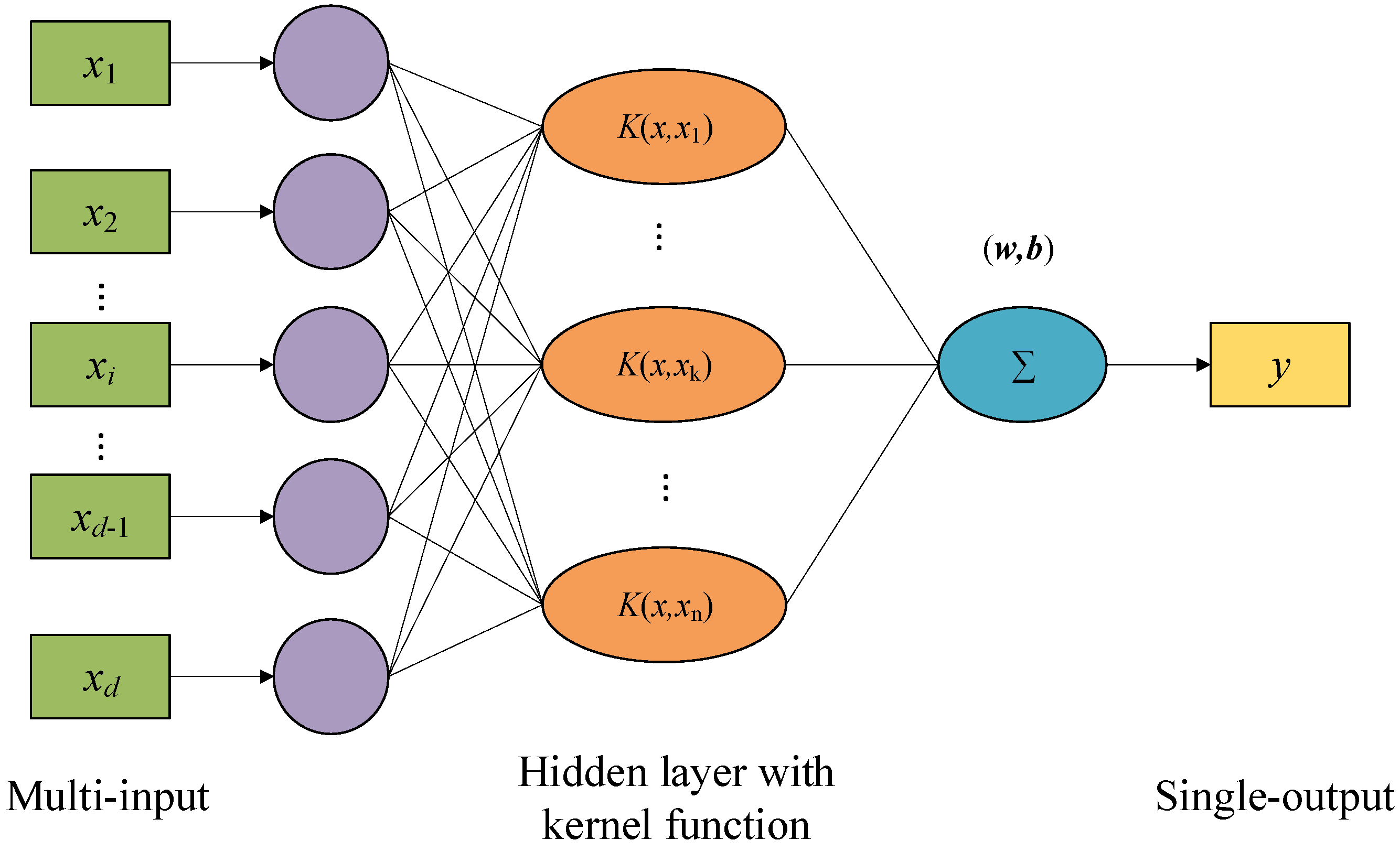
2.3. Application of Support Vector Machines for Dam Deformation Prediction

2.3.1. Single Output Least Squares Support Vector Machines

SVM [20,21] is a supervised learning algorithm based on statistical theory and the principle of structural risk minimization. The fundamental premise of the SVM is to construct an optimal decision hyperplane that maximizes the distance between the two different classes of samples that are closest to the hyperplane. In contrast to SVM, LSSVM [22,23] applies a linear least squares criterion to the loss function instead of equational constraints. The optimization problem is formulated as follows.

$$\underset{\omega ,e}{\min }\left[{\displaystyle \frac{1}{2}}{‖\omega ‖}^2+{\displaystyle \frac{1}{2}}C{\displaystyle \sum _{i=1}^N{e}_i^2}\right]$$

(9)

$$\mathrm{s}.\mathrm{t}. y_i={\omega }^T\varphi \left(x_i\right)+b+e_i,i=1,\dots ,N$$

(10)

where e_i is the error between the actual output of the ith sample and the predicted output of the ith sample.

To solve the above optimization problem, construct the Lagrangian function as follows.

$$L\left(\omega ,b,e,\alpha \right)=R\left(\omega ,e\right)-{\displaystyle \sum _{i=1}^N{\alpha }_i\left[{\omega }^T\varphi \left(x_i\right)+b+e_i-y_i\right]},i=1,\dots ,N$$

(11)

where a_i is the ith Lagrange multiplier. The regression equation for the LSSVM can be obtained by taking partial derivatives of each parameter in the respective equation and making them equal to 0. The equation is shown as follows.

$$y\left(x\right)={\omega }^T\varphi \left(x\right)+b={\displaystyle \sum _{i=1}^N{\alpha }_i}k\left(x,x_i\right)+b$$

(12)

Two significant parameters that determine the performance of LSSVM are C and γ. In order to ascertain the most appropriate parameters and prevent overfitting of the model, this study uses the PSO to optimize the kernel function parameter in the LSSVM to improve the model prediction accuracy. The PSO [31,32] relies on the comparison of the extreme values of the particles with the overall optimal solution of the particle swarm. This process is repeated, with the speed and position being constantly adjusted until the single optimal extreme value is obtained as the current global optimal solution of the entire particle swarm. The formula employed to calculate the updated speed and position is as follows.

$$\left\{\begin{array}{l}{V}_i^{\left(t+1\right)}=\omega V_i^{\left(t\right)}+c_{1}ran{d}_1\left(P_i^{\left(t\right)}-X_i^{\left(t\right)}\right)+c_{2}ran{d}_2\left(P_g^{\left(t\right)}-X_i^{\left(t\right)}\right)\\ X_i^{\left(t+1\right)}=X_i^{\left(t\right)}+V_i^{\left(t+1\right)}\end{array}\right.$$

(13)

where V_i is the velocity corresponding to the ith particle, P_i is the individual extremum of the population, P_g is the global extremum of the population, ω is the inertia weight, X_i is the position corresponding to the ith particle, c₁ and c₂ are non-negative learning factors, rand₁ and rand₂ are random numbers between [0, 1], and t is the number of current iterations.

Compared with the standard PSO, traditional PSO typically employs a fixed velocity upper limit. In this paper, the velocity boundaries are automatically calculated based on the search range, thereby avoiding the issue of unreasonable velocity settings in problems of different scales and achieving a more balanced search. For the $i-th$ particle, the velocity constraint is as follows:

$$\begin{array}{c}{V}_{i,\max }=k\cdot (X_{\max }-X_{\min })\\ V_i\in \left[-V_{i,\max },V_{i,\max }\right]\end{array}$$

(14)

where $k$ is the scaling factor, and $X_{\max }$ and $X_{\min }$ are the upper and lower bounds of the search space.

Additionally, the algorithm proposed in this paper introduces a particle mutation operation during the particle position update process. After the position update, particles are mutated with a probability $P_m=0.2$. In each iteration, when a random number $rand>0.8$, a certain dimension of the particle is reinitialized to a random value within the preset search range. This is represented as follows:

$$X_{i,k}^{(t+1)}=X_{k,\min }+(X_{k,\max }-X_{k,\min })\cdot rand,\mathrm{if} rand>0.8$$

(15)

where $k\in \left\{1,2\dots n\right\}$ represents the hyperparameters of the model.

The PSO-LSSVM model is constructed through the training of the LSSVM using the optimal parameters that have been obtained. Figure 1 shows the schematic diagram of a single-output LSSVM.

In this study, the prediction accuracy of the PSO-LSSVM model is used as a benchmark to demonstrate two key points. The first key point is the necessity of establishing a factor set considering the hysteresis effects of temperature on displacement. The second key point is the improved prediction performance achieved after performing feature selection to identify key factors compared to the performance before feature selection, which highlights the critical importance of feature selection in improving prediction accuracy.

2.3.2. Multi-Output Least Squares Support Vector Machines

The majority of existing SVM-based dam displacement prediction models are single-objective regression models, where the target variables are modeled and analyzed independently by input factors. However, such models are not applicable to multi-objective regression situations, especially in terms of how to capture potential correlation information among various target variables [53,55]. The MIMO-LSSVM model proposed in this paper is a generalization of the LSSVM model, which follows the idea of multi-objective regression to model the mutual correlation between the outputs by decomposing each weight vector ω_i (ω_i = ω₀ + v_i). In this model, each output weight vector fluctuates around a certain mean vector ω₀ and a range of variations of v_i that carry the correlation and discrepancy information, respectively. In the case of MIMO regression, the general functional form of the MIMO-LSSVM is as follows.

$$f_i\left(x\right)={\left({\omega }_0+v_i\right)}^T\varphi \left(x\right)+b_i$$

(16)

where f_i(x), ω₀ + v_i, and b_i represent the predicted values, weight vectors, and bias terms under i-dimensional outputs, respectively. Similar to the single-output support vector machine, minimizing the following objective function under the structural risk minimization principle, multi-output support vector regression can be defined as the following optimization problem.

$$\underset{{\omega }_0,V,b}{\min }J\left({\omega }_0,V,\xi \right)={\displaystyle \frac{1}{2}}{‖{\omega }_0‖}^2+{\displaystyle \frac{1}{2}}{\displaystyle \frac{\lambda }{m}}{\displaystyle \sum _{i=1}^m{v}_i^T}{v}_i+{\displaystyle \frac{1}{2}}\gamma {\displaystyle \sum _{i=1}^m{\xi }_i^T}{\xi }_i$$

(17)

$$\mathrm{s}.\mathrm{t}. Y_{i,j}={\left({\omega }_0+v_j\right)}^T\varphi \left(x_i\right)+b_j+{\xi }_{i,j}$$

(18)

where ξ is the slack variable, y_i is the i-dimensional output vector of the sample set, λ and γ are the two regularization parameters. The Lagrangian function for solving the above equation can be expressed as follows.

$$L=J\left({\omega }_0,V,\xi \right)-{\displaystyle \sum _{i=1}^m{\displaystyle \sum _{j=1}^l{A}_{i,j}^T\left[\left({\omega }_0+v_i\right)\varphi {\left(x_j\right)}^T+b_i+{\xi }_{j,i}-Y_{j,i}\right]}}$$

(19)

where $A=\left(a_1,a_2,\dots ,a_m\right)$, ${\alpha }_i$ is the Lagrange multiplier. Taking partial derivatives with respect to ω₀, V, b, ξ, and A for L, respectively, and making them equal to 0, the following system of linear equations is obtained as follows.

$$\left[\begin{array}{cc}{0}_{ml\times m}\hfill & P^T\\ \hspace{1em}P\hfill & \Omega +{\gamma }^{-1}{I}_{ml}+{\displaystyle \frac{m}{\lambda }}Q\end{array}\right]\left[\begin{array}{c}b\\ a\end{array}\right]=\left[\begin{array}{c}{0}_m\\ y\end{array}\right]$$

(20)

where P is a block matrix consisting of m all-ones vectors arranged in diagonal positions with zeros in the remaining positions, Ω is a block matrix consisting of matrix K repeated in m rows and m columns, and Q is a block matrix consisting of matrices K arranged in diagonal positions with zeros in the remaining positions. $Z=\left(\varphi \left(x_1\right),\varphi \left(x_2\right),\dots ,\varphi \left(x_l\right)\right)$, $y={\left(y_1^T,y_2^T,\dots ,y_m^T\right)}^T$, $a={\left(a_1^T,a_2^T,\dots ,a_m^T\right)}^T$, $K=Z^{T}Z$, $K_{i,j}=\varphi \left(x_i\right)\varphi \left(x_j\right)=k\left(x_i,x_j\right)$ is the element of the matrix K, and $k\left(x_i,x_j\right)$ is the kernel function.

The regression equation for MIMO-LSSVM can be expressed as follows.

$$\left\{\begin{array}{l}f\left(x\right)={\left({\omega }_0^{\ast }+v_i^{\ast }\right)}^T\varphi \left(x\right)+b_i^{\ast }={\displaystyle \sum _{i^{\prime }=1}^m{\displaystyle \sum _{j=1}^l{a}_{i^{\prime },j}^{\ast }}k\left(x,x_j\right)+\frac{m}{\lambda }{\displaystyle \sum _{j=1}^l{a}_{j,i}^{\ast }k\left(x,x_j\right)}+b_i^{\ast }}\\ k\left(x,x^{\prime }\right)=\exp \left(-p{‖x-x_i‖}^2\right) , p>0\end{array}\right.$$

(21)

where $a_{i^{\prime },j}^{\ast }$ is the jth element of $a_{i^{\prime }}^{\ast }$ in the solution vector, and $a_{i^{\prime },j}^{\ast }$ is the jth row and the ith column element of matrix A*. Similarly, the PSO is used to optimize the kernel function parameters and regularization parameters in the MIMO-LSSVM in order to obtain a higher prediction accuracy and build the MIMO-PSO-LSSVM model. Figure 2 shows the working schematic of a multi-output LSSVM.

In this paper, the optimal factor sets of different measurement points are obtained by feature selection, in which the screened-out feature factors in the same block of the dam are highly consistent. The different input factors are unified by taking the approximate number of days according to the factor set HT_AT, and then the unified factor sets of the measurement points in the same area are obtained, so that the synchronous prediction of displacement at multiple measurement points of a dam can be achieved by the MIMO-PSO-LSSVM model [35]. The established model prevents the PSO algorithm from reaching the local optimum by modifying the framework of the PSO algorithm and optimizing the single-output LSSVM model to achieve synchronous multi-output prediction. Finally, a comparison is made of the prediction performance of this multi-output model with the other single-output models, which demonstrates the superiority of the multi-output model.

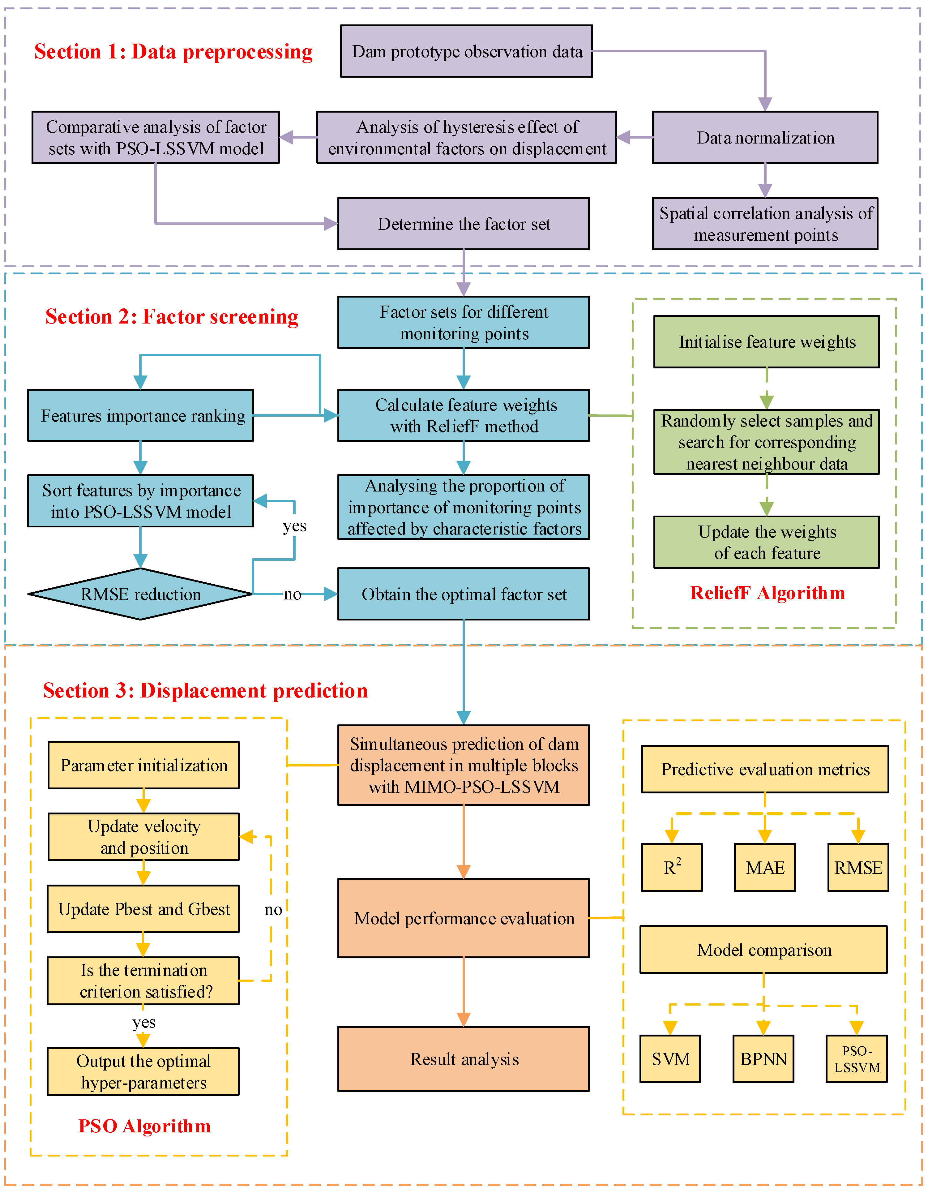
2.4. The Procedure of the Proposed Approach for Dam Health Monitoring

The procedure of the proposed approach for dam health monitoring is summarized in the flowchart in Figure 3, with the specific steps outlined as follows.

Step 1: Data collection and processing. The monitoring data of environmental variables and dam displacements are collected from the dam monitoring system, and the data are normalized.

Step 2: Determination of the hysteresis effects of environmental factors and the spatial correlation of measurement points. The sliding matching method and cosine similarity calculation method are utilized to determine the specific hysteresis times at which air temperature affects displacement at different measurement points. The correlation analysis of the displacements at different measurement points is conducted by using the maximum information coefficient method.

Step 3: Training the model for prediction after determining the model dataset. Based on the calculated specific hysteresis effects of environmental factors, the datasets of different measurement points are constructed. The first 80% of the samples are used as the training set according to the time series, and the remaining 20% are used as the testing set. Regression prediction based on PSO-LSSVM is used to select the best parameters to construct the prediction model, and the output is obtained as the preliminary prediction results.

Step 4: Screening factor sets with the feature selection method. The ReliefF algorithm is utilized to calculate the feature importance of each factor and sort the factors according to their importance. The importance of different locations of measurement points affected by the feature factors is then analyzed, and the features are added to the model for prediction according to the order of importance from the largest to the smallest. The root mean square error (RMSE) is selected as the evaluation index, and, when it reaches the minimum value, it can be considered that we have obtained the optimal factor set.

Step 5: Establishing a MIMO model for synchronous prediction of dam displacement in multiple blocks. After filtering by feature selection, a uniform factor set of measurement points in the same area is determined. The synchronous prediction of dam displacements at multiple measurement points is then realized based on the MIMO-PSO-LSSVM model.

Step 6: Comparative assessment of model performance. Three single-output prediction models, SVM, Back Propagation Neural Network (BPNN), and LSSVM optimized by PSO (PSO-LSSVM), are selected for comparative analysis with the multi-output prediction model MIMO-PSO-LSSVM. The RMSE, mean absolute error (MAE), and coefficient of determination (R²) are used to compare and evaluate the performance of the single-output prediction model and the multi-output prediction model. The mathematical expressions for these metrics are shown below.

$$RMSE=\sqrt{{\displaystyle \frac{1}{n}}{{\displaystyle \sum _{i=1}^n\left(y_m^{\left(i\right)}-y_p^{\left(i\right)}\right)}}^2}$$

(22)

$$MAE={\displaystyle \frac{1}{n}}{\displaystyle \sum _{i=1}^n\left|y_m^{\left(i\right)}-y_p^{\left(i\right)}\right|}$$

(23)

$$R^2={\displaystyle \frac{{\left({\displaystyle \sum _{i=1}^n\left(y_m^{\left(i\right)}-{\overline{y}}_m\right)\left(y_p^{\left(i\right)}-{\overline{y}}_p\right)}\right)}^2}{{\displaystyle \sum _{i=1}^n{\left(y_m^{\left(i\right)}-{\overline{y}}_m\right)}^2{\displaystyle \sum _{i=1}^n{\left(y_p^{\left(i\right)}-{\overline{y}}_p\right)}^2}}}}$$

(24)

where n is the total number of data samples, $y_m^{\left(i\right)}$ and $y_p^{\left(i\right)}$ denote the measured and predicted values of the ith data, respectively, ${\overline{y}}_m$ is the average of the measured values, and ${\overline{y}}_p$ is the average of the predicted values. Among these metrics, RMSE denotes the squared mean deviation of the predicted values from the measured values, MAE denotes the mean of the central absolute errors, and R² is a common metric for assessing the goodness of fit of the model.

3. Case Study

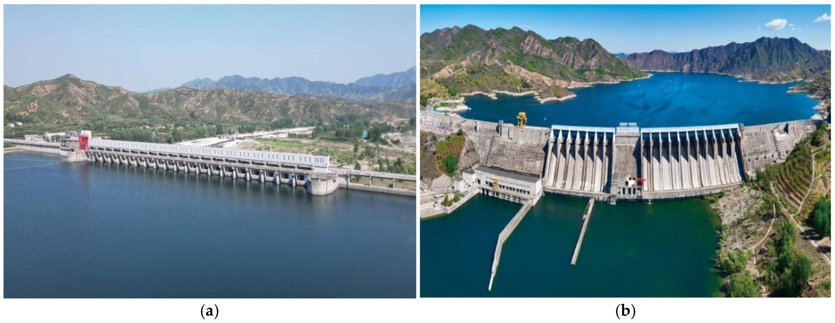
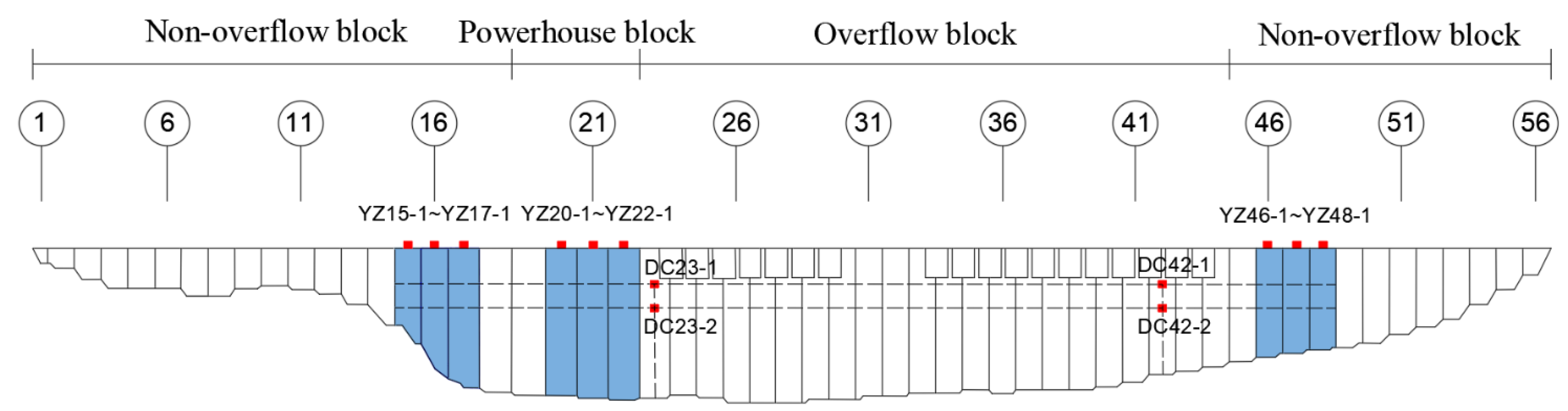
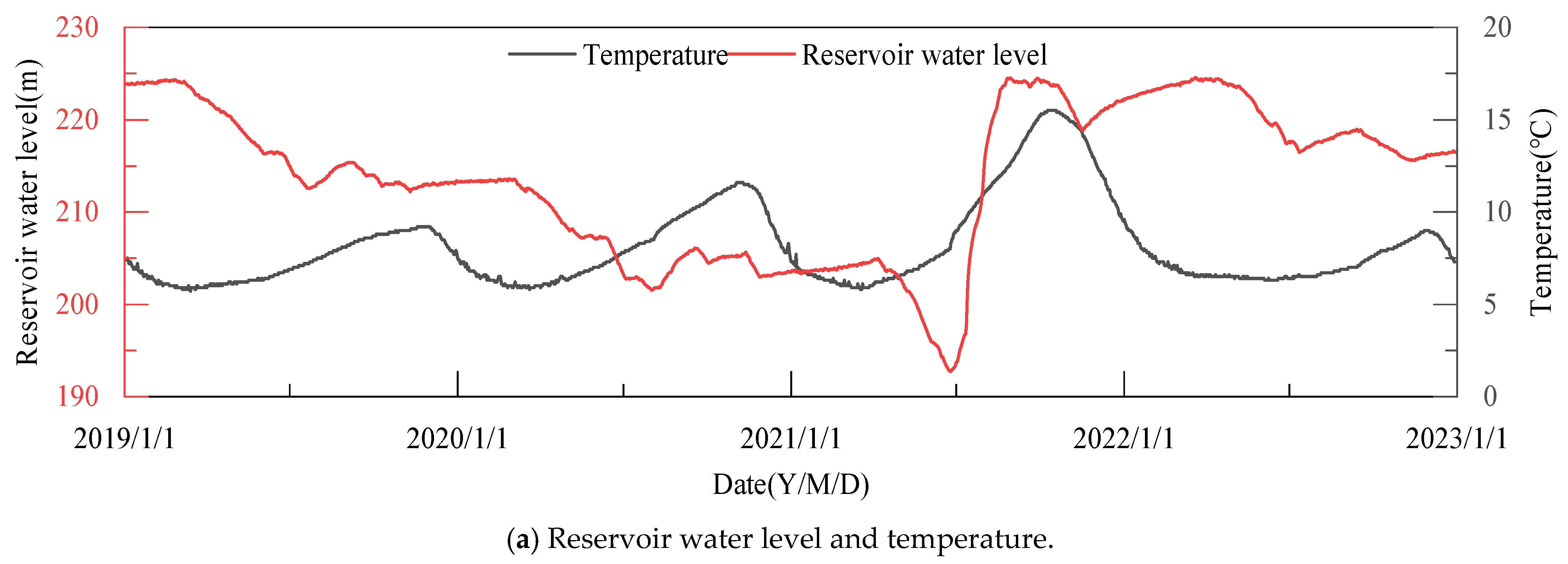
3.1. Project Overview and Data Description

The proposed method is verified using the monitoring data of a real concrete gravity dam, which has a maximum height of 107.5 m, a dam crest elevation of 230.5 m, and a total length of 1039.1 m. The upstream and downstream views of the dam are shown in Figure 4. As shown in Figure 5, the dam is divided into 56 dam sections. Sections 1 to 18 form the right bank non-overflow dam section, sections 45 to 56 form the left bank non-overflow dam section, sections 19 to 22 form the powerhouse dam section, and sections 23 to 44 form the overflow dam sections. In this study, nine measurement points are selected at the same elevation, and four measurement points are selected at different elevations, respectively. Among them, measurement points YZ15-1, YZ16-1, and YZ17-1 are selected on the right bank, measurement points YZ46-1, YZ47-1, and YZ48-1 are selected on the left bank, measurement points YZ20-1, YZ21-1, and YZ22-1 are selected on the intermediate power station dam section, and measurement points DC23-1, DC23-2, DC42-1, and DC42-2 are selected at different elevations on the overflow dam section. The dataset selected for this paper consists of 1461 sets of displacement, water level, and temperature measured from 1 January 2019 to 31 December 2022. The displacement curves of the selected dam blocks and the corresponding curves of upstream water level and air temperature are shown in Figure 6. After normalizing the monitoring data, the specific hysteresis time of temperature affecting the dam displacement can be derived by using the sliding match method and the cosine similarity calculation method, and the results are shown in Figure 7 [41].

Correlation analysis is the process of examining the relationship between two or more variables, with the aim of quantifying the strength of their association. This analysis is employed to explore the underlying patterns or rules that govern the variation of these variables. Figure 8 presents a correlation heat map, illustrating the displacements of disparate measurement points. These displacements have been calculated utilizing the maximum information coefficient method [57]. As evidenced by the figure, the correlation coefficient between each measurement point is positive. This suggests that the displacements of the measurement points exhibit a positive correlation. However, the correlation between the measurement points of different regions is expected to be low. It is evident that a high correlation coefficient exists between the displacements of measurement points in the same block, which can be maintained above 0.9, indicating a high degree of positive correlation between the displacements of the same block.

All the simulation calculations covered in this paper are computed on a Windows 11 computer equipped with an AMD Ryzen 7 6800H @ 3.20 GHz CPU, 16.0 GB of RAM, and a 64-bit processor.

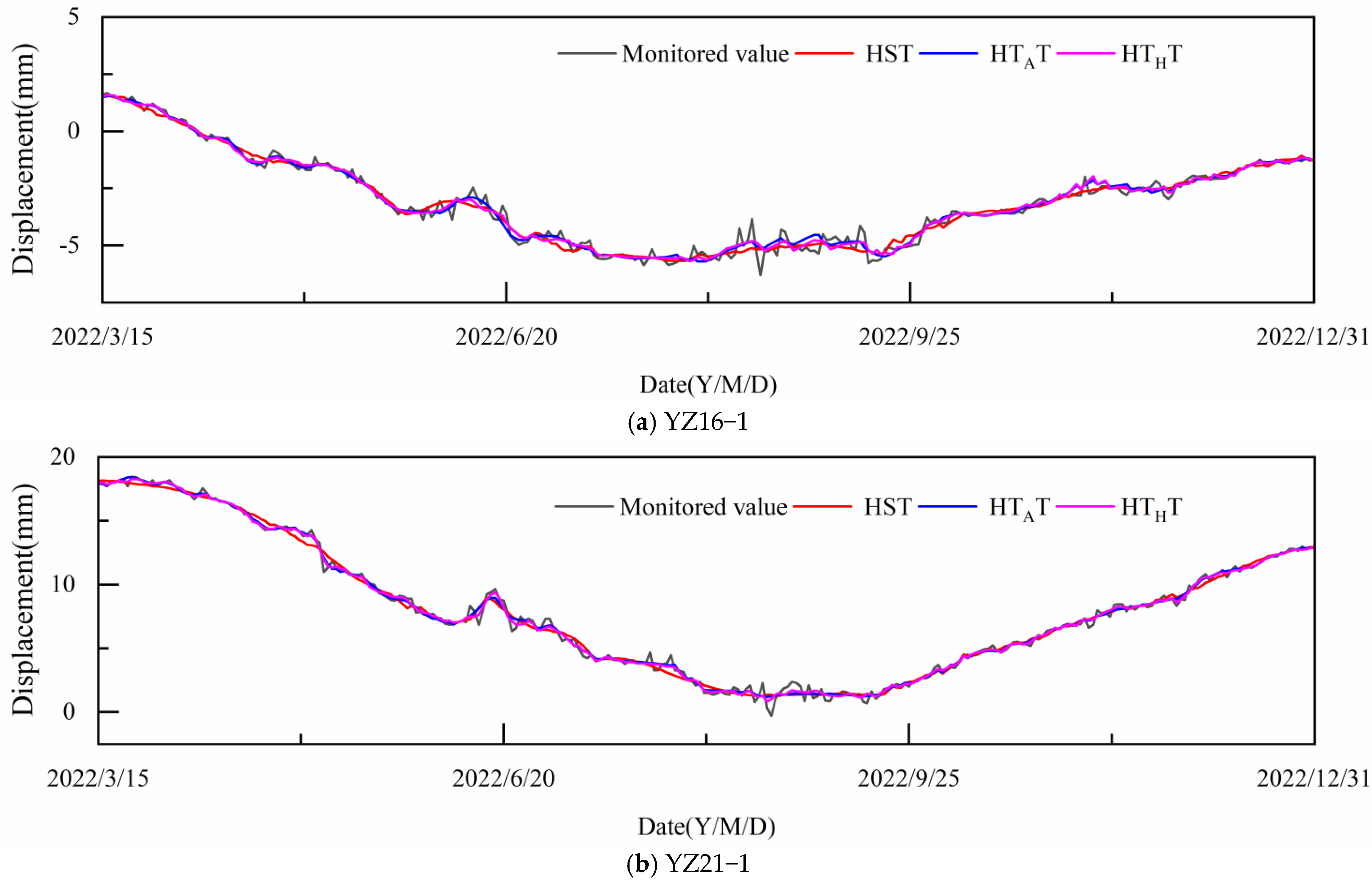
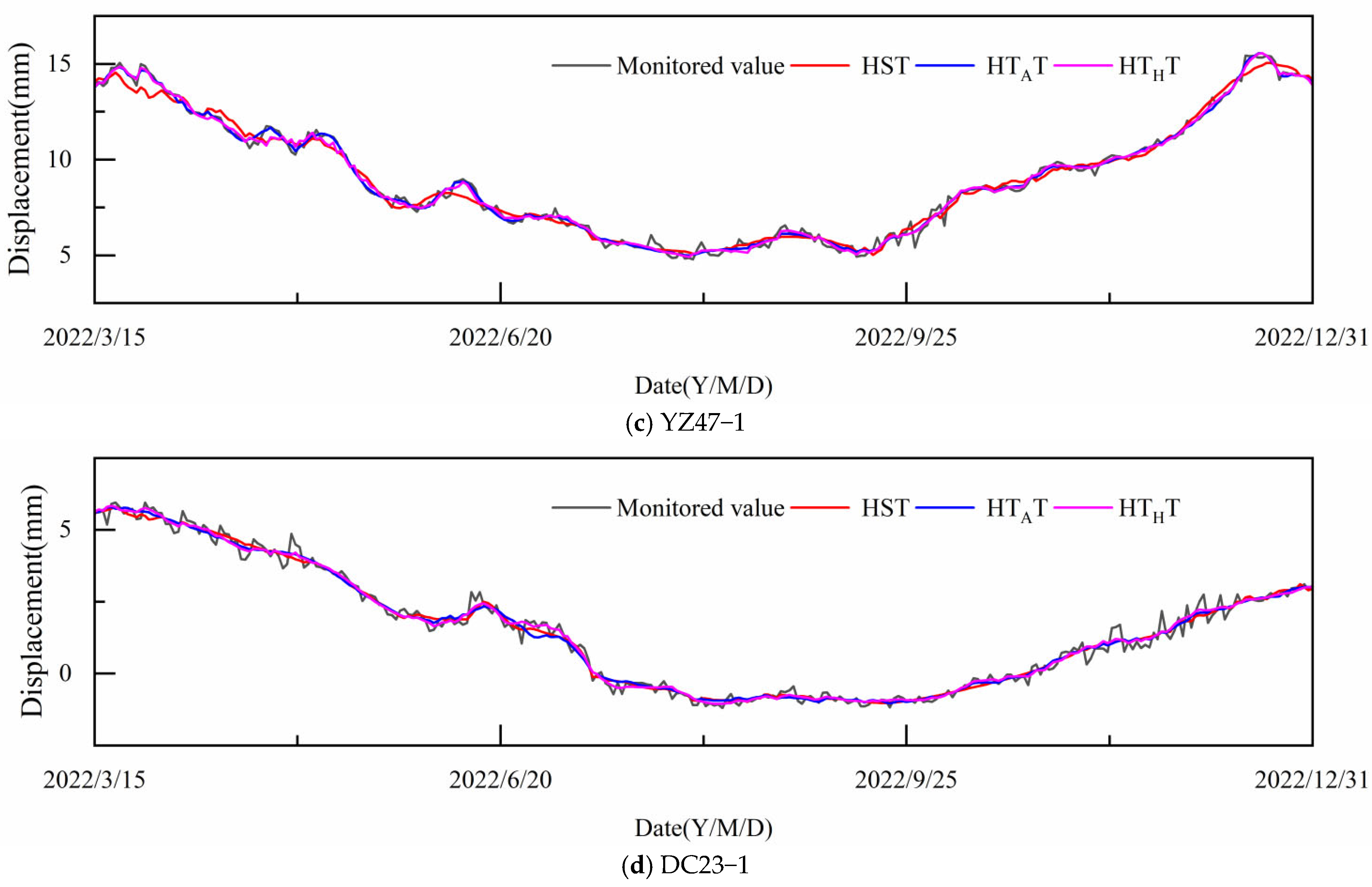
3.2. Comparative Analysis of Factor Sets

This paper mainly follows the method from reference [41], using cosine similarity to initially quantify the lag duration. Subsequently, to facilitate the establishment of a factor set for the MIMO model, the lag time is approximately set to 120 days. The traditional HST factor set and the recently proposed HT_AT factor set (a lag of 180 days is chosen for comparison in this study) are selected for comparison with the proposed HT_HT factor set in this paper, and the constructed factor sets are shown in

Table 2. Comparison of different factor sets.

Factor Sets	Factors
HST	$\left\{H^1\right.,H^2,H^3,\sin \left({\displaystyle \frac{2\pi t}{365}}\right),\cos \left({\displaystyle \frac{2\pi t}{365}}\right),\sin \left({\displaystyle \frac{4\pi t}{365}}\right),\cos \left({\displaystyle \frac{4\pi t}{365}}\right),\theta ,\left.\ln \theta \right\}$
HTAT	$\left\{H^1\right.,H^2,H^3,T_0,T_{1-2},T_{3-7},T_{8-15},T_{16-30},T_{31-60},T_{61-90},T_{91-120},T_{121-180},\theta ,\left.\ln \theta \right\}$
HTHT	$\left\{H^1\right.,H^2,H^3,T_0,T_{1-2},T_{3-7},T_{8-15},T_{16-30},T_{31-60},T_{61-90},T_{91-120},\theta ,\left.\ln \theta \right\}$

. A total of 13 measurement points are selected to predict displacement under the single-output PSO-LSSVM model with different factor sets. The average value of the prediction performance of all the measurement points is taken as the evaluation index to compare the prediction accuracy under different factor sets. The results of the analyses are shown in Figure 9. In each area, a single representative measurement point is selected to plot the displacement prediction fitting curve. The prediction results are displayed in Figure 10. The analysis indicates that the proposed HT_HT factor set demonstrates the highest prediction accuracy. Compared with the HST factor set, the average enhancement rate in the HT_HT factor set of R², MAE, and RMSE has reached 0.60%, 25.59%, and 22.10%, respectively. In subsequent studies, the HT_HT factor set, which considers the hysteresis effect of temperature on displacement, will be employed in the analysis.

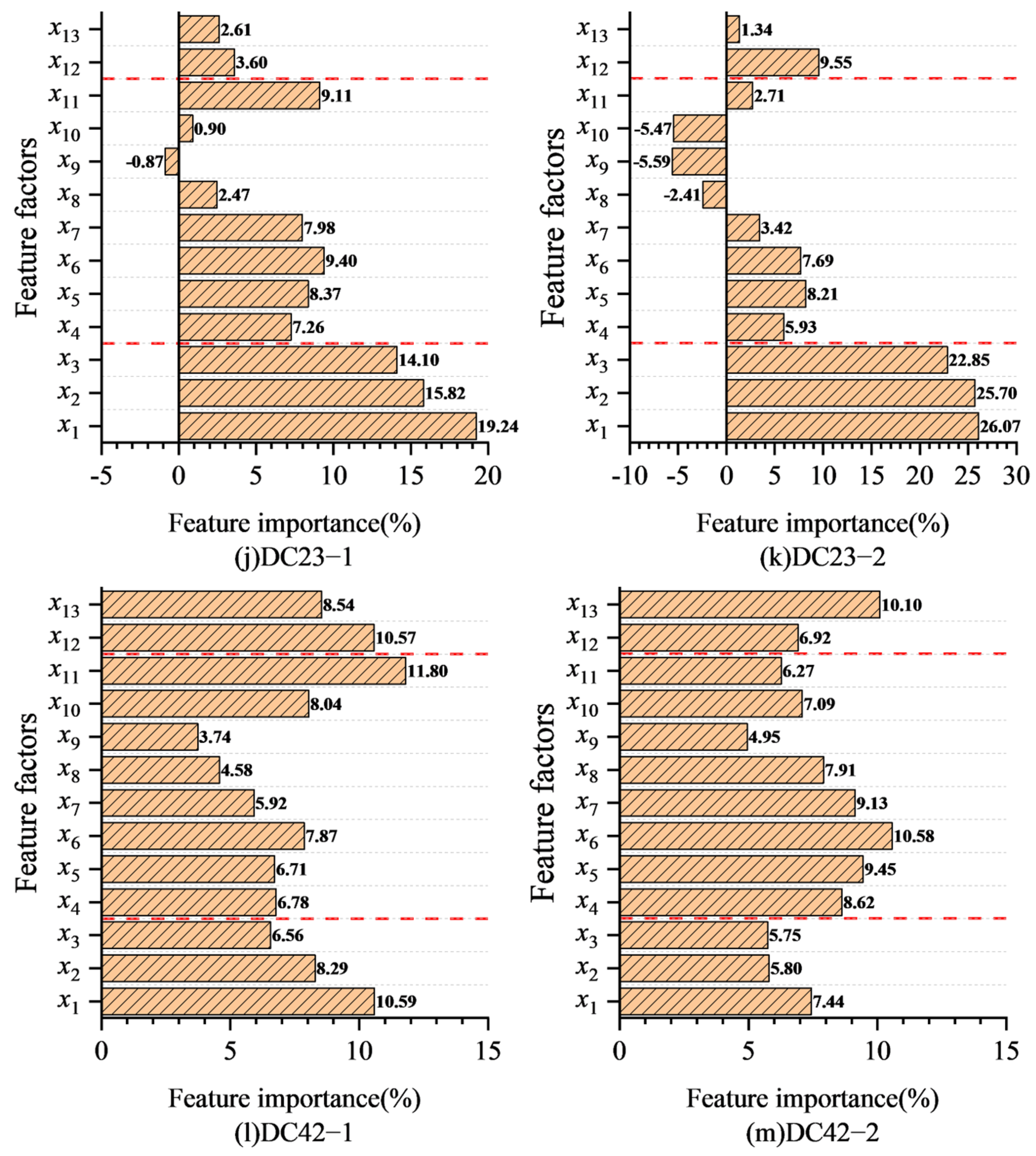
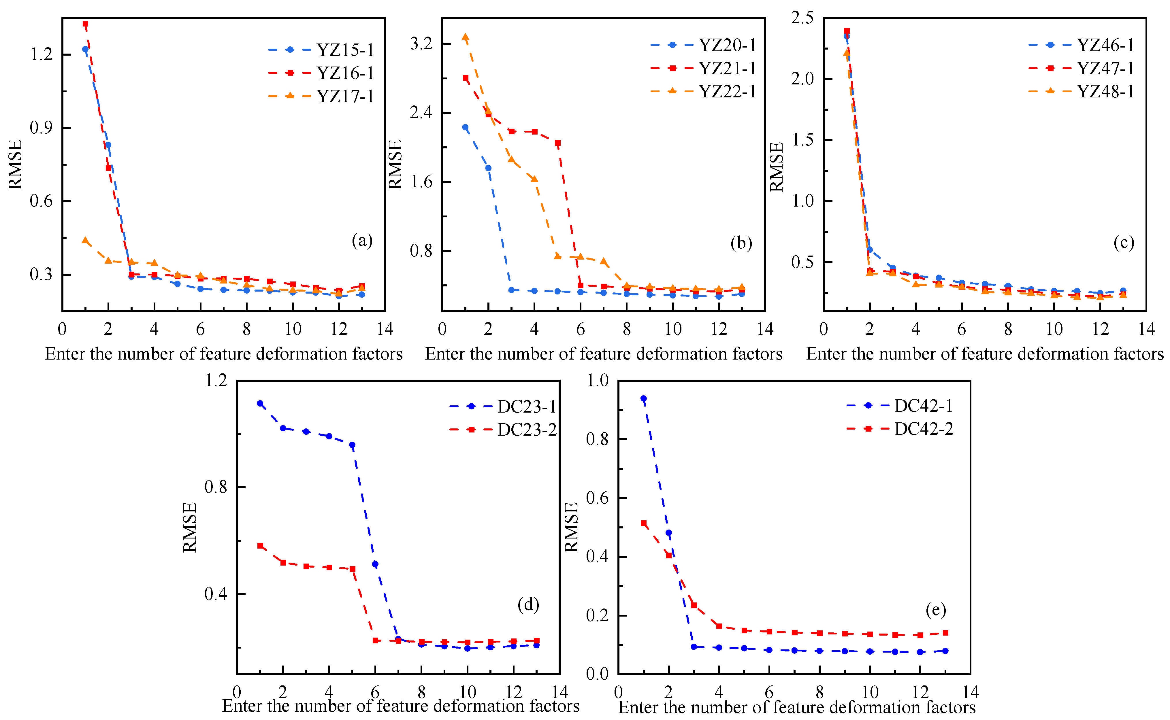
3.3. Screening the Main Factor Set with Feature Selection Method

Following the determination of the HT_HT factor set, the importance of the features in the factor set needs to be analyzed. During the construction of the model, the input features have a substantial impact on the performance of the model. Deformation prediction models map complex non-linear relationships between deformations and features. The introduction of redundant features into the model can potentially result in overfitting. Conversely, an insufficient number of features may result in the model disregarding potential relationships between the data, leading to underfitting. In this paper, the ReliefF feature selection method is employed to rank the importance of input features in the factor set for feature screening.

The feature importance ranking of different measurement points is calculated by the ReliefF feature selection method, and it is evident that there is a consistent trend in the feature importance ranking of measurement points in the same area. The results are shown in Figure 11. It can be assumed that the temperature factor exerts a greater influence on dam displacement in the non-overflow dam section, while the hydraulic pressure factor has a greater effect on dam displacement in the overflow dam section. Furthermore, the percentage of characteristic importance of neighboring points is found to be similar. At the same elevation, the points of neighboring dam sections demonstrate a high degree of consistency in the percentage of characteristic importance. In different elevations, the close vertical distance between two measurement points of different elevations in the studied example leads to similar characteristics of the two measurement points. This results in the percentage of characteristic importance of the two measurement points being similar, which is in line with the conclusions of the reference [58].

According to the order of feature importance derived for different measurement points from the largest to the smallest, the features are sequentially input into the PSO-LSSVM model for training and testing. The input factor set with the smallest RMSE value is selected as the optimal factor set after feature filtering. The results of the analyses for each measurement point are presented in Figure 12. Following a thorough analysis, it can be concluded that, when fewer factors are employed, the RMSE is comparatively large. This is due to the fact that the input factors of the model do not contain sufficient information to accurately reflect the nonlinear characteristics of the dam deformation. Conversely, when all factors with high feature importance are used as input to the model, the RMSE of the model decreases significantly and reaches its lowest point. If the number of factors is further increased, the RMSE of the testing and training sets will tend to increase continuously. This is because the redundant information should have a negative effect on the performance of the model. Therefore, based on the results presented in Figure 12, the optimal sets of feature factors for different measurement points are selected, as illustrated in

Table 3. Optimal factor sets for different measurement points.

Measurement Points	Factor Sets
YZ15-1-YZ17-1	$\left\{H\right.,H^2,H^3,T_0,T_{1-2},T_{3-7},T_{8-15},T_{16-30},T_{61-90},T_{91-120},\theta ,\left.\ln \theta \right\}$
YZ20-1-YZ22-1	$\left\{H\right.,H^2,H^3,T_0,T_{1-2},T_{3-7},T_{8-15},T_{31-60},T_{61-90},T_{91-120},\theta ,\left.\ln \theta \right\}$
YZ46-1-YZ48-1	$\left\{H\right.,H^2,H^3,T_0,T_{1-2},T_{3-7},T_{8-15},T_{16-30},T_{31-60},T_{61-90},T_{91-120},\left.\theta \right\}$
DC23-1-DC23-2	$\left\{H\right.,H^2,H^3,T_0,T_{1-2},T_{3-7},T_{8-15},T_{91-120},\left.\theta ,\ln \theta \right\}$
DC42-1-DC42-2	$\left\{H\right.,H^2,H^3,T_0,T_{1-2},T_{3-7},T_{8-15},T_{16-30},T_{61-90},T_{91-120}\left.,\theta ,\ln \theta \right\}$

.

Take four measurement points (YZ16-1, YZ21-1, YZ47-1, and DC23-1) to plot the displacement prediction fitting curve graph; the prediction value before and after the feature selection is compared with the real value, and the analysis results are shown in Figure 13 and

Table 4. Comprehensive performance evaluation indicators before and after feature selection.

Measurement Point	Without Feature Selection			With Feature Selection
	R2	MAE/(mm)	RMSE/(mm)	R2	MAE/(mm)	RMSE/(mm)
YZ15-1	0.9816	0.1475	0.2183	0.9826 (0.11%)	0.1447 (1.84%)	0.2122 (2.78%)
YZ16-1	0.9825	0.1723	0.2546	0.9852 (0.28%)	0.1534 (11.01%)	0.2348 (7.78%)
YZ17-1	0.9905	0.1555	0.2423	0.9921 (0.17%)	0.1421 (8.61%)	0.2204 (9.05%)
YZ20-1	0.9951	0.2082	0.3010	0.9961 (0.10%)	0.1881 (9.66%)	0.2700 (10.33%)
YZ21-1	0.9953	0.2434	0.3522	0.9959 (0.06%)	0.2301 (5.54%)	0.3295 (6.44%)
YZ22-1	0.9950	0.2544	0.3760	0.9956 (0.06%)	0.2415 (5.10%)	0.3519 (6.40%)
YZ46-1	0.9930	0.2069	0.2687	0.9940 (0.10%)	0.1861 (10.05%)	0.2487 (7.46%)
YZ47-1	0.9938	0.1803	0.2424	0.9950 (0.12%)	0.1657 (8.09%)	0.2194 (9.49%)
YZ48-1	0.9936	0.1772	0.2293	0.9946 (0.10%)	0.1562 (11.85%)	0.2099 (8.45%)
DC23-1	0.9901	0.1540	0.2092	0.9912 (0.12%)	0.1457 (5.35%)	0.1968 (5.95%)
DC23-2	0.9597	0.1743	0.2267	0.9620 (0.24%)	0.1653 (5.16%)	0.2202 (2.87%)
DC42-1	0.9982	0.0576	0.0794	0.9984 (0.03%)	0.0525 (8.86%)	0.0757 (4.65%)
DC42-2	0.9823	0.0855	0.1417	0.9843 (0.20%)	0.0789 (7.77%)	0.1335 (5.79%)
Average	0.9885	0.1705	0.2417	0.99106923076923198 (0.13%)	0.233784615384615577 (7.52%)	0.29210769230769248 (6.97%)

Note: Values in parentheses refer to the percentage enhancement in model performance with feature selection relative to model performance without feature selection.

. It has been determined through analysis that the prediction accuracy is further enhanced following the implementation of feature selection. Compared with the factor sets without feature selection, the average enhancement rate of each measurement point in R², MAE, and RMSE has reached 0.13%, 7.52%, and 6.97%, respectively. It can be concluded that the utilization of feature selection methods for the purpose of factor screening is both reasonable and feasible.

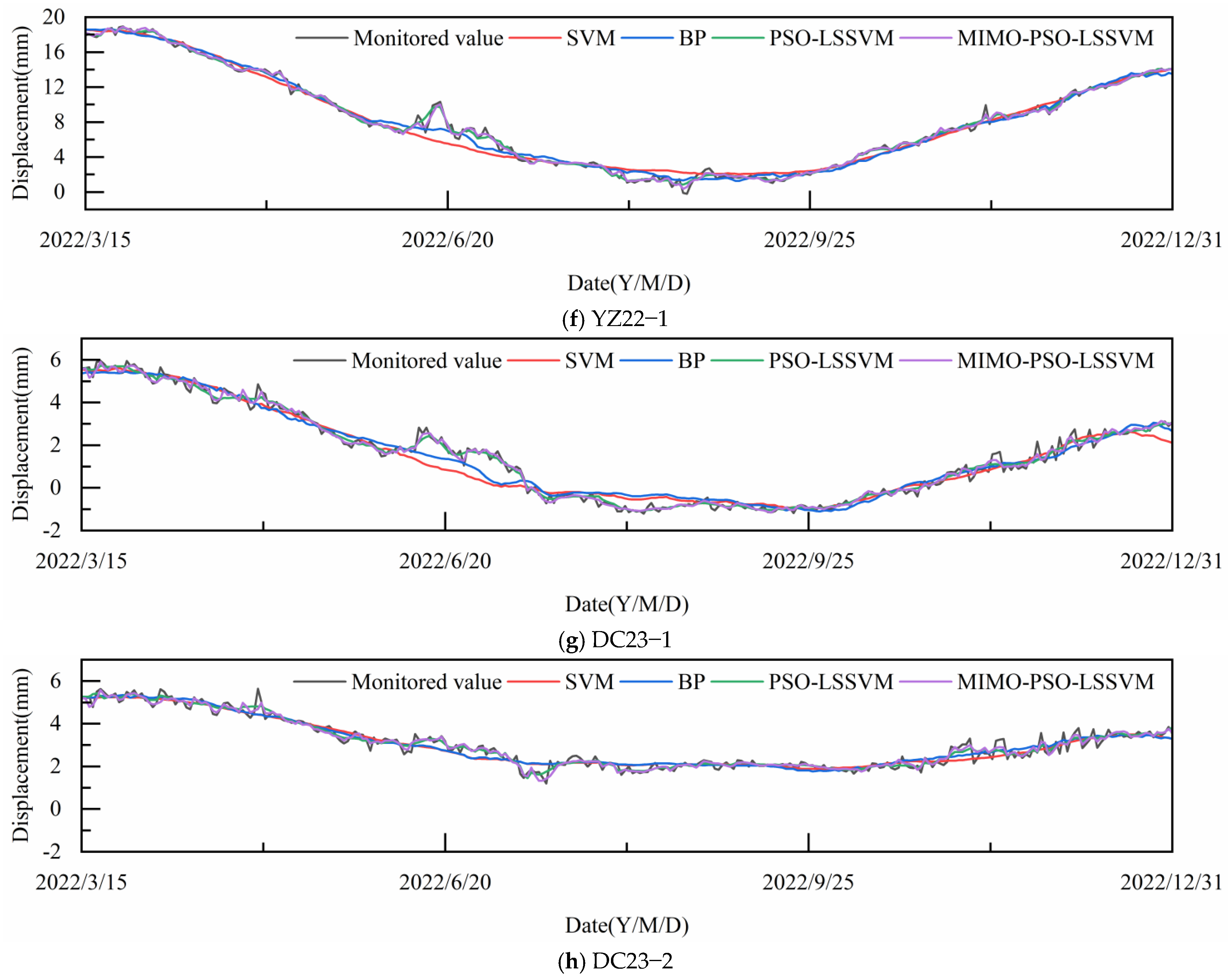
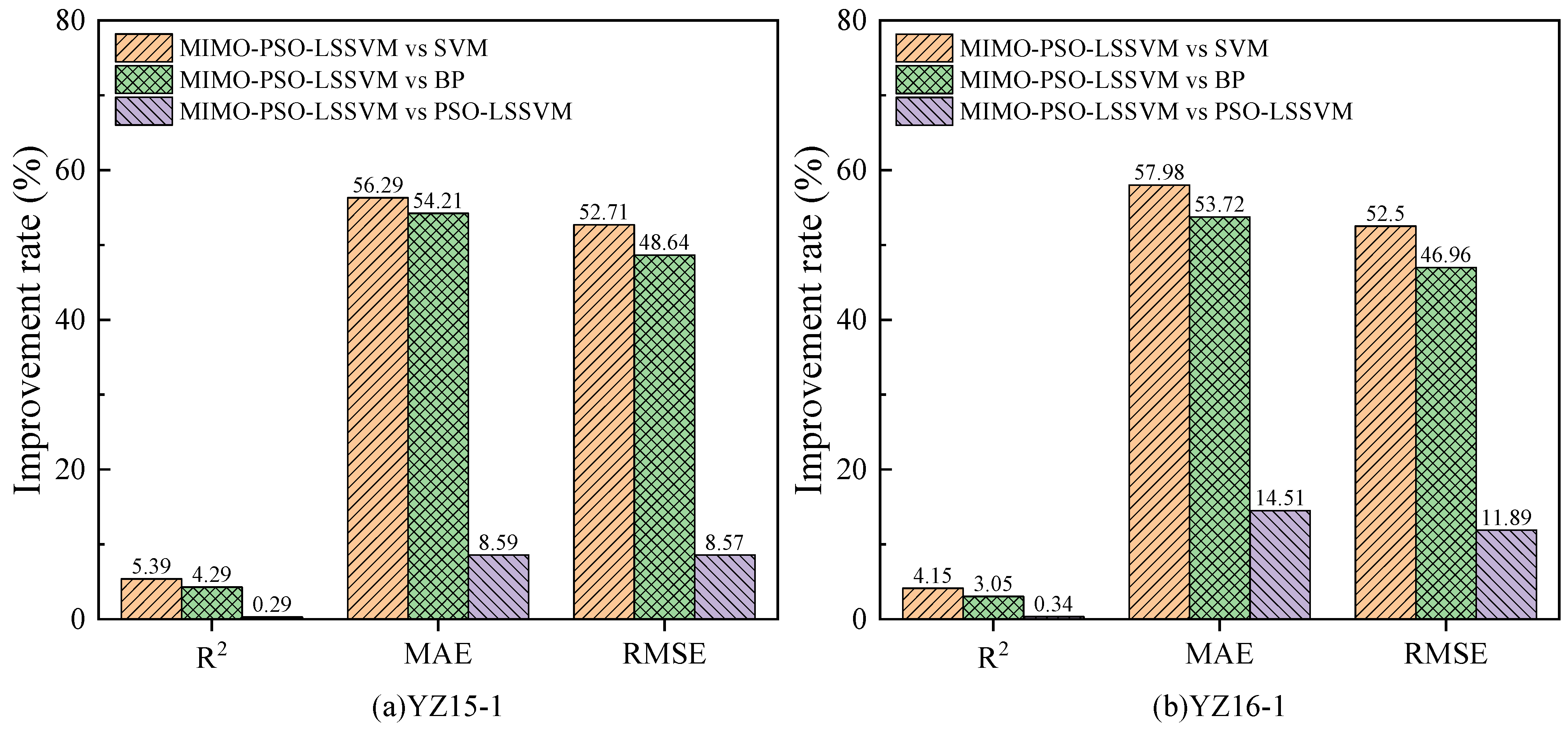
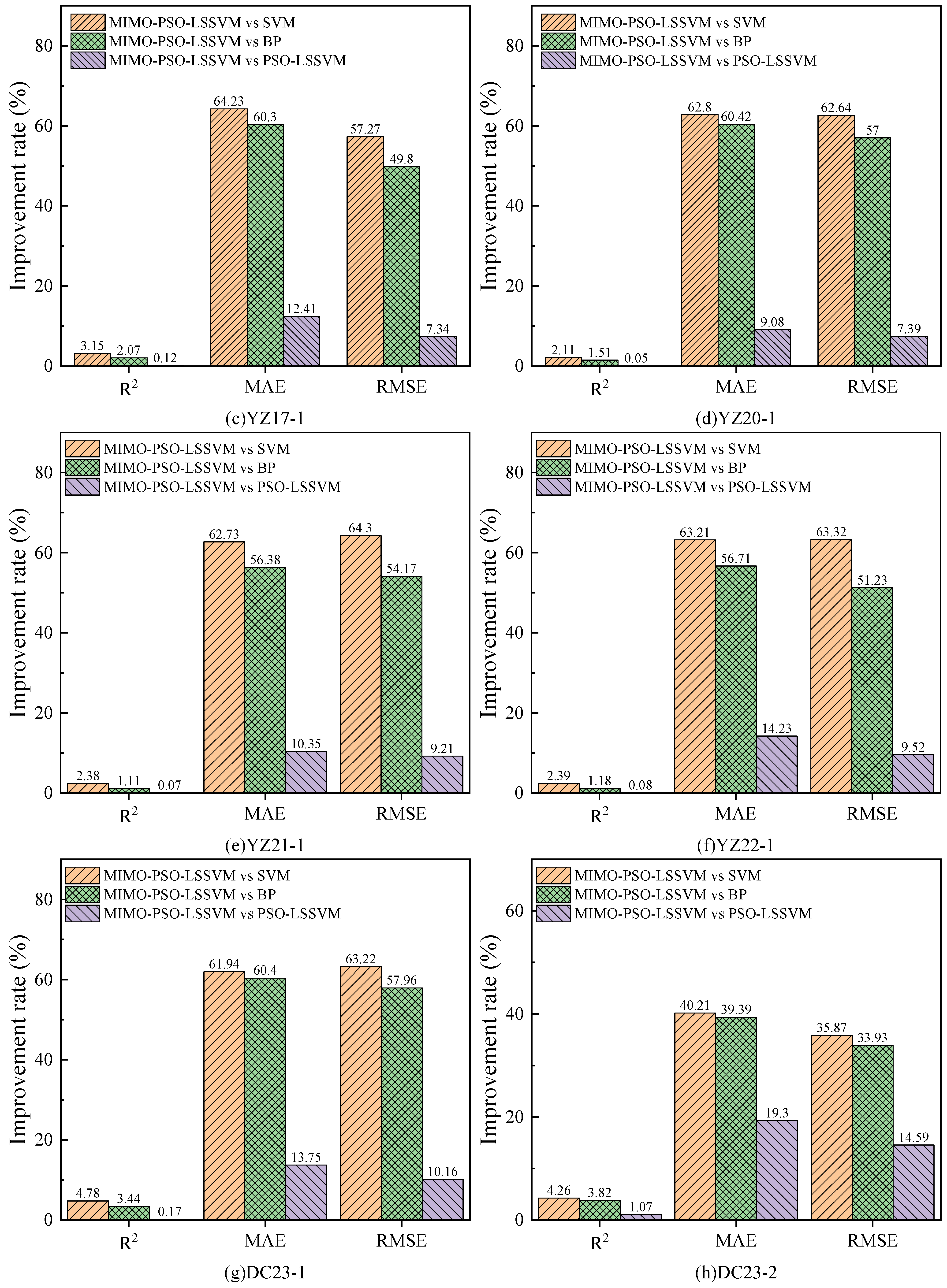
3.4. Synchronous Prediction with Multiple Inputs and Multiple Outputs Model

Following the determination of the unified factor set, the trained MIMO-PSO-LSSVM model can be utilized to achieve the synchronous prediction of the displacement of the same dam block. In this paper, three prediction models, SVM, BPNN, and PSO-LSSVM, are selected as comparison models for the MIMO-PSO-LSSVM model. The computational parameters of the BPNN model are set as follows: the maximum number of training iterations is set to 1000, the learning rate is 0.1, and a default sigmoid function is employed between the input and hidden layers. The computational parameters of the SVM model are set as follows: the radial basis kernel function g takes the value of 0.8, and the penalty factor c takes the value of 4.0. The computational parameters of the PSO-LSSVM model are set as follows: the SVM adopts the least squares learning algorithm and uses the radial basis kernel function, the PSO optimization algorithm is chosen to determine the penalty parameters and the radial basis kernel function parameters, the initial population size of the PSO algorithm is set to 20, the maximum number of iterations is 300, the inertia factor ω is set to 0.8, and the learning factors c₁ and c₂ are set to 2. The computational parameters of the MIMO-PSO-LSSVM model are set as follows: the penalty parameter, the regularisation parameter, and the radial basis kernel function parameter take values ranging from 0.01 to 15, and the PSO optimization algorithm is chosen to determine these parameters; the initial population size of the PSO algorithm is taken to be 20, the maximum number of iterations is 300, the inertia factor ω takes the value of 0.8, and the learning factors c₁ and c₂ take the value of 2.

As illustrated in Figure 14, the performance of the four prediction models, SVM, BPNN, PSO-LSSVM, and MIMO-PSO-LSSVM, is evaluated through eight measurement points. These eight measurement points comprise the non-overflow dam block measurement points YZ15-1, YZ16-1, and YZ17-1, the overflow dam block measurement points YZ20-1, YZ21-1, and YZ22-1, and the different elevation measurement points DC23-1 and DC23-2. It can be observed that all the models capture the main trends of the displacement changes of the dam block, with the MIMO-PSO-LSSVM model predicting the closest to the true value of the displacement, while the PSO-LSSVM model is the next closest, and the BPNN and SVM models predicting the worst.

The comparison of the comprehensive performance evaluation metrics under different prediction models is shown in

Table 5. Comprehensive performance evaluation indicators under different prediction models.

Measurement Point	Prediction Model	R2	MAE/(mm)	RMSE/(mm)
YZ15-1	SVM	0.9351 (−5.39%)	0.3027 (−56.29%)	0.4102 (−52.71%)
	BPNN	0.9450 (−4.29%)	0.2889 (−54.21%)	0.3777 (−48.64%)
	PSO-LSSVM	0.9826 (−0.29%)	0.1447 (−8.59%)	0.2122 (−8.57%)
	MIMO-PSO-LSSVM	0.9855 (0%)	0.1323 (0%)	0.1940 (0%)
YZ16-1	SVM	0.9492 (−4.15%)	0.3120 (−57.98%)	0.4356 (−52.50%)
	BPNN	0.9593 (−3.05%)	0.2833 (−53.72%)	0.3901 (−46.96%)
	PSO-LSSVM	0.9852 (−0.34%)	0.1534 (−14.51%)	0.2348 (−11.89%)
	MIMO-PSO-LSSVM	0.9886 (0%)	0.1311 (0%)	0.2069 (0%)
YZ17-1	SVM	0.9630 (−3.15%)	0.3481 (−64.23%)	0.4779 (−57.27%)
	BPNN	0.9732 (−2.07%)	0.3136 (−60.30%)	0.4068 (−49.80%)
	PSO-LSSVM	0.9921 (−0.12%)	0.1421 (−12.41%)	0.2204 (−7.34%)
	MIMO-PSO-LSSVM	0.9933 (0%)	0.1245 (0%)	0.2042 (0%)
YZ20-1	SVM	0.9760 (−2.11%)	0.4597 (−62.80%)	0.6691 (−62.64%)
	BPNN	0.9818 (−1.51%)	0.4320 (−60.42%)	0.5814 (−57.00%)
	PSO-LSSVM	0.9961 (−0.05%)	0.1881 (−9.08%)	0.2700 (−7.39%)
	MIMO-PSO-LSSVM	0.9966 (0%)	0.1710 (0%)	0.2500 (0%)
YZ21-1	SVM	0.9734 (−2.38%)	0.5535 (−62.73%)	0.8382 (−64.30%)
	BPNN	0.9857 (−1.11%)	0.4730 (−56.38%)	0.6149 (−54.17%)
	PSO-LSSVM	0.9959 (−0.07%)	0.2301 (−10.35%)	0.3295 (−9.21%)
	MIMO-PSO-LSSVM	0.9966 (0%)	0.2063 (0%)	0.2992 (0%)
YZ22-1	SVM	0.9731 (−2.39%)	0.5630 (−63.21%)	0.8681 (−63.32%)
	BPNN	0.9848 (−1.18%)	0.4784 (−56.71%)	0.6528 (−51.23%)
	PSO-LSSVM	0.9956 (−0.08%)	0.2415 (−14.23%)	0.3519 (−9.52%)
	MIMO-PSO-LSSVM	0.9964 (0%)	0.2071 (0%)	0.3184 (0%)
DC23-1	SVM	0.9476 (−4.78%)	0.3303 (−61.94%)	0.4807 (−63.22%)
	BPNN	0.9599 (−3.44%)	0.3174 (−60.40%)	0.4206 (−57.96%)
	PSO-LSSVM	0.9912 (−0.17%)	0.1457 (−13.75%)	0.1968 (−10.16%)
	MIMO-PSO-LSSVM	0.9929 (0%)	0.1257 (0%)	0.1768 (0%)
DC23-2	SVM	0.9326 (−4.26%)	0.2231 (−40.21%)	0.2933 (−35.87%)
	BPNN	0.9365 (−3.82%)	0.2201 (−39.39%)	0.2847 (−33.93%)
	PSO-LSSVM	0.9620 (−1.07%)	0.1653 (−19.30%)	0.2202 (−14.59%)
	MIMO-PSO-LSSVM	0.9723 (0%)	0.1334 (0%)	0.1881 (0%)

Note: Values in parentheses refer to the reduction percentage in performance of the single-output model relative to the multi-output model, respectively. Bold values indicate the optimal value of the indicator.

. Each model is benchmarked against the proposed MIMO-PSO-LSSVM model. The analysis is conducted based on the average data obtained from eight measurement points. Compared with the SVM model, the MIMO-PSO-LSSVM model achieves an improvement of 3.56%, 60.18%, and 58.92%, in terms of R², MAE, and RMSE, respectively. Compared with the BPNN model, the MIMO-PSO-LSSVM model achieves an improvement of 2.54%, 56.13%, and 51.22%, in terms of R², MAE, and RMSE, respectively. Compared with the PSO-LSSVM model, the MIMO-PSO- LSSVM model achieves an improvement of 0.27%, 12.72%, and 9.74%, in terms of R², MAE, and RMSE, respectively. The enhancement effect is illustrated in Figure 15. This result demonstrates that when predicting multiple datasets with high correlation, the prediction accuracy of the traditional single-output model is inferior to that of the proposed MIMO-PSO-LSSVM model. This is due to the fact that the MIMO-PSO-LSSVM model takes into account the potential spatial correlation between the displacement data, thus enhancing the prediction accuracy.

Furthermore, the MIMO-PSO-LSSVM model has been shown to exhibit superiority over the single-output PSO-LSSVM model with regard to prediction efficiency. To illustrate this, consider the non-overflow dam section measurement points YZ15-1, YZ16-1, and YZ17-1. The MIMO-PSO-LSSVM model requires approximately 203 s to predict all the measurement points, whereas the single-output PSO-LSSVM model requires approximately 614 s, which is about three times higher in terms of speed. This is due to the capacity of the MIMO-PSO-LSSVM model to predict the displacements of multiple measurement points synchronously, thereby markedly enhancing the computational efficiency in comparison with the single-output PSO-LSSVM prediction model. Although the SVM and BPNN models, which serve as comparison models, consume minimal time for prediction, their prediction accuracy shows a significant gap compared with the multi-output model due to the absence of optimization algorithms. Therefore, a comparative analysis of prediction efficiency between these models and the multi-output model is not considered.

In summary, the MIMO-PSO-LSSVM model has been demonstrated to enhance prediction accuracy and efficiency when compared with other single-output prediction models, and it can be concluded that it is a reliable and excellent prediction method.

4. Conclusions

In this paper, a new factor set considering the hysteresis effect of temperature on displacement is proposed. The optimal factor set is formed by screening the main factors with the ReliefF according to the prediction accuracy of the PSO-LSSVM model as the index. The correlation between measurement points is then taken into account, and a MIMO displacement prediction model for concrete gravity dams is established by the LSSVM optimized by PSO, which achieves the synchronous prediction of the displacement of multiple measurement points. This process enables the establishment of a MIMO considering correlation and hysteresis prediction method for gravity dam displacement with interpretable functions. The feasibility and superiority of the method are verified by measured data of a concrete gravity dam in North China, and the main conclusions obtained are summarized as follows.

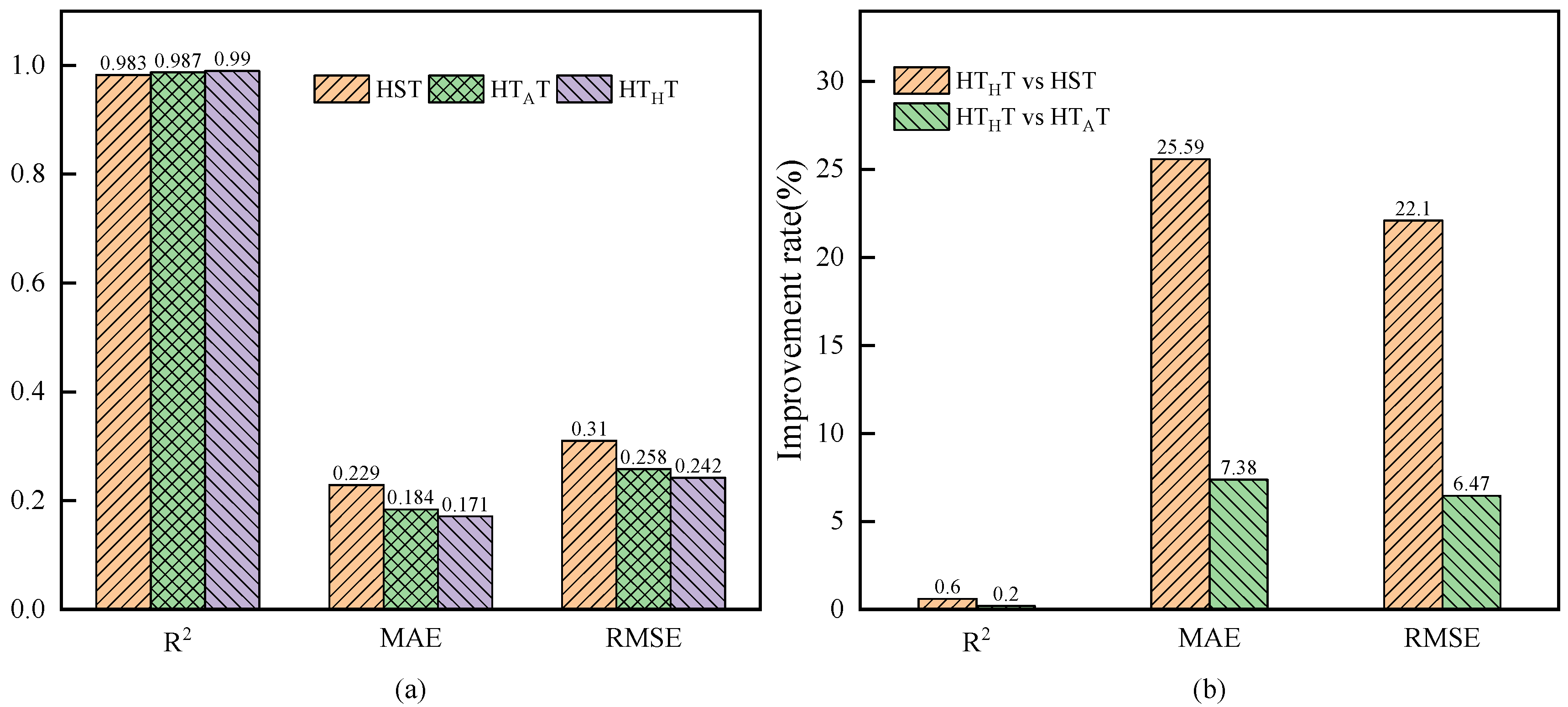
• The specific times at which the temperature at different measurement points exhibits hysteresis effects on the displacement of gravity dams are determined through the utilization of the sliding match method and the cosine similarity calculation method. A factor set that considers the hysteresis effect of temperature on displacement is obtained, and the prediction accuracy of the PSO-LSSVM model is used as an index to compare with the other factor sets. This demonstrated the necessity to consider the hysteresis effect of the environmental factors on the displacement of gravity dams.
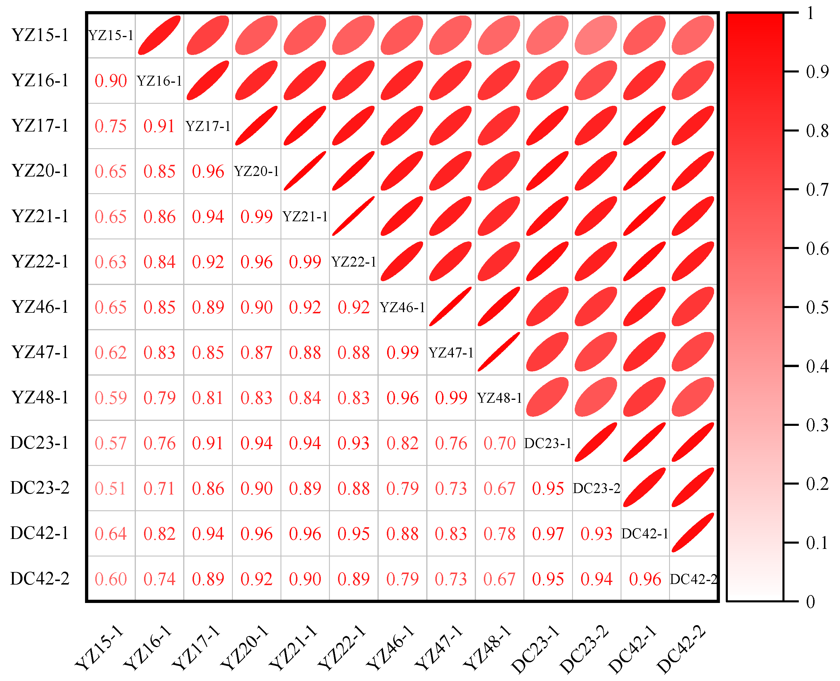
• Through the ReliefF feature selection method, the importance of each feature is found to be similar for the displacements at the measurement points in the same area, for instance, the influence of temperature on the dam displacement is greater in the non-overflow dam section, while the influence of hydraulic pressure on the dam displacement is greater in the overflow dam section. Furthermore, the implementation of a filtering process on the features of the factor set resulted in an enhancement of the model’s prediction accuracy, thereby highlighting the significance of feature selection in the context of predicting dam displacements.
• A MIMO synchronous prediction model, MIMO-PSO-LSSVM, that considers the potential spatial correlation between measurement points is proposed. Compared with the contrastive models, this MIMO-PSO-LSSVM model is able to take into account the potential spatial correlation between the displacement measured data, thereby improving the prediction accuracy. Furthermore, the model exhibits the advantage of being able to predict displacements at multiple measurement points simultaneously, resulting in a significant efficiency improvement over the single-output PSO-LSSVM model.

The method proposed in this paper, with slight modifications, can be applied to predict other monitoring metrics of gravity dams, such as seepage, stress, and strain, as well as the relevant monitoring quantities of other types of dams, including arch dams and earth-rock dams. Concrete dams can be regarded as highly non-stationary systems, and the use of a static lag window to quantify the duration of lag presents certain limitations. Future research will investigate methods for dynamically calibrating lag times based on seasonal variations. Meanwhile, considering that the model treats all output dimensions equally during computation, assuming that each output contributes equally to the task without applying differential weights, future work will explore the introduction of an output weighting mechanism to assign different importance weights to different outputs. Future research will also explore the feasibility of using transfer learning, retraining, or retraining with fewer samples for the MIMO-PSO-LSSVM model. Additionally, the feasibility of applying the method proposed in this paper to strain prediction and damage detection in concrete structures will also be explored [59,60].

References

1. Li, Z.; Jiang, W.G.; Hou, P.; Peng, K.F.; Deng, Y.W.; Wang, X.Y. Changes in the ecosystem service importance of the seven major river basins in China during the implementation of the Millennium development goals (2000–2015) and sustainable development goals (2015–2020). J. Clean. Prod. 2023, 433, 139787. [Google Scholar] [CrossRef]
2. Liu, D.H.; Chen, J.J.; Hu, D.J.; Zhang, Z. Dynamic BIM-augmented UAV safety inspection for water diversion project. Comput. Ind. 2019, 108, 163–177. [Google Scholar] [CrossRef]
3. Sevieri, G.; De Falco, A. Dynamic structural health monitoring for concrete gravity dams based on the Bayesian inference. J. Civ. Struct. Health Monit. 2020, 10, 235–250. [Google Scholar] [CrossRef]
4. Shao, C.F.; Zheng, S.; Gu, C.S.; Hu, Y.T.; Qin, X.N. A novel outlier detection method for monitoring data in dam engineering. Expert Syst. Appl. 2022, 193, 116476. [Google Scholar] [CrossRef]
5. Ren, Q.B.; Li, M.C.; Li, H.; Song, L.G.; Si, W.; Liu, H. A robust prediction model for displacement of concrete dams subjected to irregular water level fluctuations. Comput.-Aided Civ. Infrastruct. Eng. 2021, 36, 577–601. [Google Scholar] [CrossRef]
6. Li, B.; Yang, J.; Hu, D.X. Dam monitoring data analysis methods: A literature review. Struct. Control Health Monit. 2020, 27, e2501. [Google Scholar] [CrossRef]
7. Liu, X.Y.; Li, Z.C.; Sun, L.S.; Khailah, E.Y.; Wang, J.J.; Lu, W.G. A critical review of statistical model of dam monitoring data. J. Build. Eng. 2023, 80, 108106. [Google Scholar] [CrossRef]
8. Stojanovic, B.; Milivojevic, M.; Ivanovic, M. Adaptive system for dam behavior modeling based on linear regression and genetic algorithms. Adv. Eng. Softw. 2013, 65, 182–190. [Google Scholar] [CrossRef]
9. Mata, J.; De Castro, A.T.; De Castro, J.S. Constructing statistical models for arch dam deformation. Struct. Control Health Monit. 2014, 21, 423–437. [Google Scholar] [CrossRef]
10. Xi, G.Y.; Yue, J.P.; Zhou, B.X.; Pu, T. Application of an artificial immune algorithm on a statistical model of dam displacement. Comput. Math. Appl. 2011, 62, 3980–3986. [Google Scholar] [CrossRef]
11. Yu, H.; Wu, Z.R.; Bao, T.F.; Zhang, L. Multivariate analysis in dam monitoring data with PCA. Sci. China-Technol. Sci. 2010, 53, 1088–1097. [Google Scholar] [CrossRef]
12. Xu, C.; Yue, D.; Deng, C.F. Hybrid GA/SIMPLS as alternative regression model in dam deformation analysis. Eng. Appl. Artif. Intell. 2012, 25, 468–475. [Google Scholar] [CrossRef]
13. Wang, S.W.; Gu, C.S.; Liu, Y.; Gu, H.; Xu, B.; Wu, B.B. Displacement observation data-based structural health monitoring of concrete dams: A state-of-art review. Structures 2024, 68, 107072. [Google Scholar] [CrossRef]
14. Ma, C.H.; Yang, J.; Zenz, G.; Staudacher, E.J.; Cheng, L. Calibration of the microparameters of the discrete element method using a relevance vector machine and its application to rockfill materials. Adv. Eng. Softw. 2020, 147, 102833. [Google Scholar] [CrossRef]
15. Kang, F.; Li, J.J.; Zhao, S.Z.; Wang, Y.J. Structural health monitoring of concrete dams using long-term air temperature for thermal effect simulation. Eng. Struct. 2019, 180, 642–653. [Google Scholar] [CrossRef]
16. Chauhan, V.K.; Dahiya, K.; Sharma, A. Problem formulations and solvers in linear SVM: A review. Artif. Intell. Rev. 2019, 52, 803–855. [Google Scholar] [CrossRef]
17. Kang, F.; Liu, J.; Li, J.J.; Li, S.J. Concrete dam deformation prediction model for health monitoring based on extreme learning machine. Struct. Control Health Monit. 2017, 24, e1997. [Google Scholar] [CrossRef]
18. Wen, Z.P.; Zhou, R.L.; Su, H.Z. MR and stacked GRUs neural network combined model and its application for deformation prediction of concrete dam. Expert Syst. Appl. 2022, 201, 117272. [Google Scholar] [CrossRef]
19. Xu, B.; Chen, Z.Y.; Wang, X.; Bu, J.W.; Zhu, Z.H.; Zhang, H.; Wang, S.D.; Lu, J.Y. Combined prediction model of concrete arch dam displacement based on cluster analysis considering signal residual correction. Mech. Syst. Signal Process. 2023, 203, 110721. [Google Scholar] [CrossRef]
20. Xing, Y.; Chen, Y.; Huang, S.P.; Wang, P.; Xiang, Y.F. Research on dam deformation prediction model based on optimized SVM. Processes 2022, 10, 1842. [Google Scholar] [CrossRef]
21. Su, H.Z.; Chen, Z.X.; Wen, Z.P. Performance improvement method of support vector machine-based model monitoring dam safety. Struct. Control Health Monit. 2016, 23, 252–266. [Google Scholar] [CrossRef]
22. Kisi, O.; Parmar, K.S. Application of least square support vector machine and multivariate adaptive regression spline models in long term prediction of river water pollution. J. Hydrol. 2016, 534, 104–112. [Google Scholar] [CrossRef]
23. Cheng, L.; Zheng, D.J. Two online dam safety monitoring models based on the process of extracting environmental effect. Adv. Eng. Softw. 2013, 57, 48–56. [Google Scholar] [CrossRef]
24. Katoch, S.; Chauhan, S.S.; Kumar, V. A review on genetic algorithm: Past, present, and future. Multimed. Tools Appl. 2021, 80, 8091–8126. [Google Scholar] [CrossRef]
25. Cheng, J.H.; Shi, T. Structural optimization of transmission line tower based on improved fruit fly optimization algorithm. Comput. Electr. Eng. 2022, 103, 108320. [Google Scholar] [CrossRef]
26. Xu, L.; Wen, Z.P.; Su, H.Z.; Cola, S.; Fabbian, N.; Fen, Y.M.; Yang, S.S. An innovative method integrating two deep learning networks and hyperparameter optimization for identifying fiber optic temperature measurements in earth-rock dams. Adv. Eng. Softw. 2025, 199, 103802. [Google Scholar] [CrossRef]
27. Saremi, S.; Mirjalili, S.; Lewis, A. Grasshopper optimisation algorithm: Theory and application. Adv. Eng. Softw. 2017, 105, 30–47. [Google Scholar] [CrossRef]
28. Wang, D.S.; Tan, D.P.; Liu, L. Particle swarm optimization algorithm: An overview. Soft Comput. 2018, 22, 387–408. [Google Scholar] [CrossRef]
29. Khatir, A.; Capozucca, R.; Khatir, S.; Magagnini, E.; Benaissa, B.; Le Thanh, C.; Wahab, M.A. A new hybrid PSO-YUKI for double cracks identification in CFRP cantilever beam. Compos. Struct. 2023, 311, 116803. [Google Scholar] [CrossRef]
30. Ouadi, B.; Khatir, A.; Magagnini, E.; Mokadem, M.; Abualigah, L.; Smerat, A. Optimizing silt density index prediction in water treatment systems using pressure-based gradient boosting hybridized with Salp Swarm Algorithm. J. Water Process Eng. 2024, 68, 106479. [Google Scholar] [CrossRef]
31. Wang, S.D.; Xu, B.; Zhu, Z.H.; Li, J.; Lu, J.Y. Reliability analysis of concrete gravity dams based on least squares support vector machines with an improved particle swarm optimization algorithm. Appl. Sci. 2022, 12, 12315. [Google Scholar] [CrossRef]
32. Kang, F.; Li, J.S.; Li, J.J. System reliability analysis of slopes using least squares support vector machines with particle swarm optimization. Neurocomputing 2016, 209, 46–56. [Google Scholar] [CrossRef]
33. Milillo, P.; Perissin, D.; Salzer, J.T.; Lundgren, P.; Lacava, G.; Milillo, G.; Serio, C. Monitoring dam structural health from space: Insights from novel InSAR techniques and multi-parametric modeling applied to the Pertusillo dam Basilicata, Italy. Int. J. Appl. Earth Obs. Geoinf. 2016, 52, 221–229. [Google Scholar] [CrossRef]
34. Tatin, M.; Briffaut, M.; Dufour, F.; Simon, A.; Fabre, J.P. Thermal displacements of concrete dams: Accounting for water temperature in statistical models. Eng. Struct. 2015, 91, 26–39. [Google Scholar] [CrossRef]
35. Kang, F.; Li, J.J.; Dai, J.H. Prediction of long-term temperature effect in structural health monitoring of concrete dams using support vector machines with Jaya optimizer and salp swarm algorithms. Adv. Eng. Softw. 2019, 131, 60–76. [Google Scholar] [CrossRef]
36. Kang, F.; Liu, X.; Li, J.J. Temperature effect modeling in structural health monitoring of concrete dams using kernel extreme learning machines. Struct. Health Monit.-Int. J. 2020, 19, 987–1002. [Google Scholar] [CrossRef]
37. Zhang, J.H.; Wang, J.; Chai, L.S. Factors influencing hysteresis characteristics of concrete dam deformation. Water Sci. Eng. 2017, 10, 166–174. [Google Scholar] [CrossRef]
38. Xu, B.; Zhang, H.; Xia, H.; Song, D.L.; Zhu, Z.H.; Chen, Z.Y.; Lu, J.Y. A multi-level prediction model of concrete dam displacement considering time hysteresis and residual correction. Meas. Sci. Technol. 2025, 36, 015107. [Google Scholar] [CrossRef]
39. Yu, X.; Li, J.J.; Kang, F. A hybrid model of bald eagle search and relevance vector machine for dam safety monitoring using long-term temperature. Adv. Eng. Inform. 2023, 55, 101863. [Google Scholar] [CrossRef]
40. Wang, S.W.; Xu, Y.L.; Gu, C.S.; Bao, T.F.; Xia, Q.; Hu, K. Hysteretic effect considered monitoring model for interpreting abnormal deformation behavior of arch dams: A case study. Struct. Control Health Monit. 2019, 26, e2417. [Google Scholar] [CrossRef]
41. Ren, Q.B.; Li, M.C.; Song, L.G.; Liu, H. An optimized combination prediction model for concrete dam deformation considering quantitative evaluation and hysteresis correction. Adv. Eng. Inform. 2020, 46, 101154. [Google Scholar] [CrossRef]
42. Huang, B.; Kang, F.; Li, J.J.; Wang, F. Displacement prediction model for high arch dams using long short-term memory based encoder-decoder with dual-stage attention considering measured dam temperature. Eng. Struct. 2023, 280, 115686. [Google Scholar] [CrossRef]
43. Dai, B.; Gu, C.S.; Zhao, E.F.; Qin, X.N. Statistical model optimized random forest regression model for concrete dam deformation monitoring. Struct. Control Health Monit. 2018, 25, e2170. [Google Scholar] [CrossRef]
44. Xu, B.; Chen, Z.Y.; Su, H.Z.; Zhang, H. A deep learning method for predicting the displacement of concrete arch dams considering the effect of cracks. Adv. Eng. Inform. 2024, 62, 102547. [Google Scholar] [CrossRef]
45. Robnik-Šikonja, M.; Kononenko, I. Theoretical and empirical analysis of ReliefF and RReliefF. Mach. Learn. 2003, 53, 23–69. [Google Scholar] [CrossRef]
46. Luo, H.; Han, J.Q. Trace ratio criterion based large margin subspace learning for feature selection. IEEE Access 2019, 7, 6461–6472. [Google Scholar] [CrossRef]
47. Zhang, H.; Xu, B.; Chen, Z.Y. A novel reconstruction method for displacement missing data of arch dam via hierarchical clustering and deep learning. Eng. Appl. Artif. Intell. 2024, 133, 108586. [Google Scholar] [CrossRef]
48. Li, Y.L.; Min, K.Y.; Zhang, Y. Prediction of the failure point settlement in rockfill dams based on spatial-temporal data and multiple-monitoring-point models. Eng. Struct. 2021, 243, 112658. [Google Scholar] [CrossRef]
49. Chen, B.; Hu, T.Y.; Huang, Z.S.; Fang, C.H. A spatio-temporal clustering and diagnosis method for concrete arch dams using deformation monitoring data. Struct. Health Monit.-Int. J. 2019, 18, 1355–1371. [Google Scholar] [CrossRef]
50. Wang, S.W.; Xu, C.; Liu, Y.; Wu, B.B. A spatial association-coupled double objective support vector machine prediction model for diagnosing the deformation behaviour of high arch dams. Struct. Health Monit.-Int. J. 2022, 21, 945–964. [Google Scholar] [CrossRef]
51. Rodríguez-Pérez, R.; Bajorath, J. Interpretation of machine learning models using shapley values: Application to compound potency and multi-target activity predictions. J. Comput.-Aided Mol. Des. 2020, 34, 1013–1026. [Google Scholar] [CrossRef]
52. Li, Y.T.; Bao, T.F.; Chen, Z.X.; Gao, Z.X.; Shu, X.S.; Zhang, K. A missing sensor measurement data reconstruction framework powered by multi-task Gaussian process regression for dam structural health monitoring systems. Measurement 2021, 186, 110085. [Google Scholar] [CrossRef]
53. Chen, S.Y.; Gu, C.S.; Lin, C.N.; Hariri-Ardebili, M.A. Prediction of arch dam deformation via correlated multi-target stacking. Appl. Math. Model. 2021, 91, 1175–1193. [Google Scholar] [CrossRef]
54. Li, S.J.; Zhao, H.B.; Ru, Z.L.; Sun, Q.C. Probabilistic back analysis based on Bayesian and multi-output support vector machine for a high cut rock slope. Eng. Geol. 2016, 203, 178–190. [Google Scholar] [CrossRef]
55. Ren, Q.B.; Li, H.; Zheng, X.Z.; Li, M.C.; Xiao, L.; Kong, T. Multi-block synchronous prediction of concrete dam displacements using MIMO machine learning paradigm. Adv. Eng. Inform. 2023, 55, 101855. [Google Scholar] [CrossRef]
56. Wu, Z.R. Safety Monitoring Theory and Its Application of Hydraulic Structures; Higher Education Press: Beijing, China, 2003. (In Chinese) [Google Scholar]
57. Reshef, D.N.; Reshef, Y.A.; Finucane, H.K.; Grossman, S.R.; Mcvean, G.; Turnbaugh, P.J.; Lander, E.S.; Mitzenmacher, M.; Sabeti, P.C. Detecting novel associations in large data sets. Science 2011, 334, 1518–1524. [Google Scholar] [CrossRef]
58. Zhang, Y.; Zhong, W.; Li, Y.L.; Wen, L.F. A deep learning prediction model of DenseNet-LSTM for concrete gravity dam deformation based on feature selection. Eng. Struct. 2023, 295, 116827. [Google Scholar] [CrossRef]
59. Khatir, A.; Capozucca, R.; Khatir, S.; Magagnini, E.; Benaissa, B.; Cuong-Le, T. An efficient improved gradient boosting for strain prediction in near-surface mounted fiber-reinforced polymer strengthened reinforced concrete beam. Front. Struct. Civ. Eng. 2024, 18, 1148–1168. [Google Scholar] [CrossRef]
60. Khatir, A.; Capozucca, R.; Khatir, S.; Magagnini, E.; Cuong-Le, T. Enhancing Damage Detection Using Reptile Search Algorithm-Optimized Neural Network and Frequency Response Function. J. Vib. Eng. Technol. 2025, 13, 88. [Google Scholar] [CrossRef]
Figure 1. General architecture of single-output support vector machine.
Applsci 15 07096 g001
Figure 2. General architecture of multi-output support vector machine.
Applsci 15 07096 g002
Figure 3. Flowchart of dam displacement prediction.
Applsci 15 07096 g003
Figure 4. The concrete gravity dam: (a) upstream view; (b) downstream view.
Applsci 15 07096 g004
Figure 5. Layout of the dam displacement monitoring system.
Applsci 15 07096 g005
Figure 6. The process lines of environmental variables and measuring displacements.
Applsci 15 07096 g006aApplsci 15 07096 g006b
Figure 7. Specific hysteresis time during which the temperature affects the displacements.
Applsci 15 07096 g007
Figure 8. Correlation analysis of the selected dam section displacement.
Applsci 15 07096 g008
Figure 9. Prediction performance histogram: (a) performance metrics; (b) comparison of performance improvement.
Applsci 15 07096 g009
Figure 10. The fitting curve graph for the comparison of model prediction performance.
Applsci 15 07096 g010aApplsci 15 07096 g010b
Figure 11. Importance weights of features at different measurement points.
Applsci 15 07096 g011aApplsci 15 07096 g011b
Figure 12. Curves of RMSE with different feature inputs: (a) YZ15−1, YZ16−1, YZ17−1; (b) YZ20−1, YZ21−1, YZ22−1; (c) YZ46−1, YZ47−1, YZ48−1; (d) DC23−1, DC23−2; (e) DC42−1, DC42−2.
Applsci 15 07096 g012
Figure 13. Comparison of model prediction performance before and after feature selection.
Applsci 15 07096 g013
Figure 14. Comparison of predicted dam displacements using different prediction models.
Applsci 15 07096 g014aApplsci 15 07096 g014b
Figure 15. Comparison of the performance improvement rate of different prediction models.
Applsci 15 07096 g015aApplsci 15 07096 g015b