
Defect R-CNN: A Novel High-Precision Method for CT Image Defect Detection

 ,
,
Abstract
1. Introduction
2. Methods
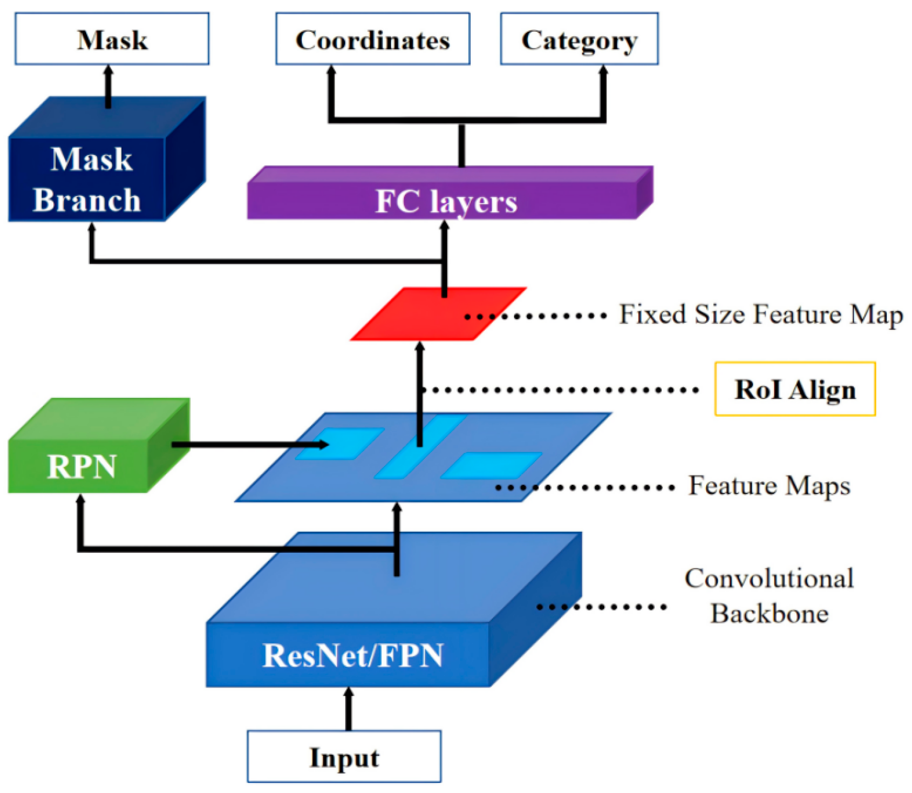
2.1. Mask R-CNN
2.2. Analysis of Model Complexity
2.2.1. Model Parameters
2.2.2. Computational Load
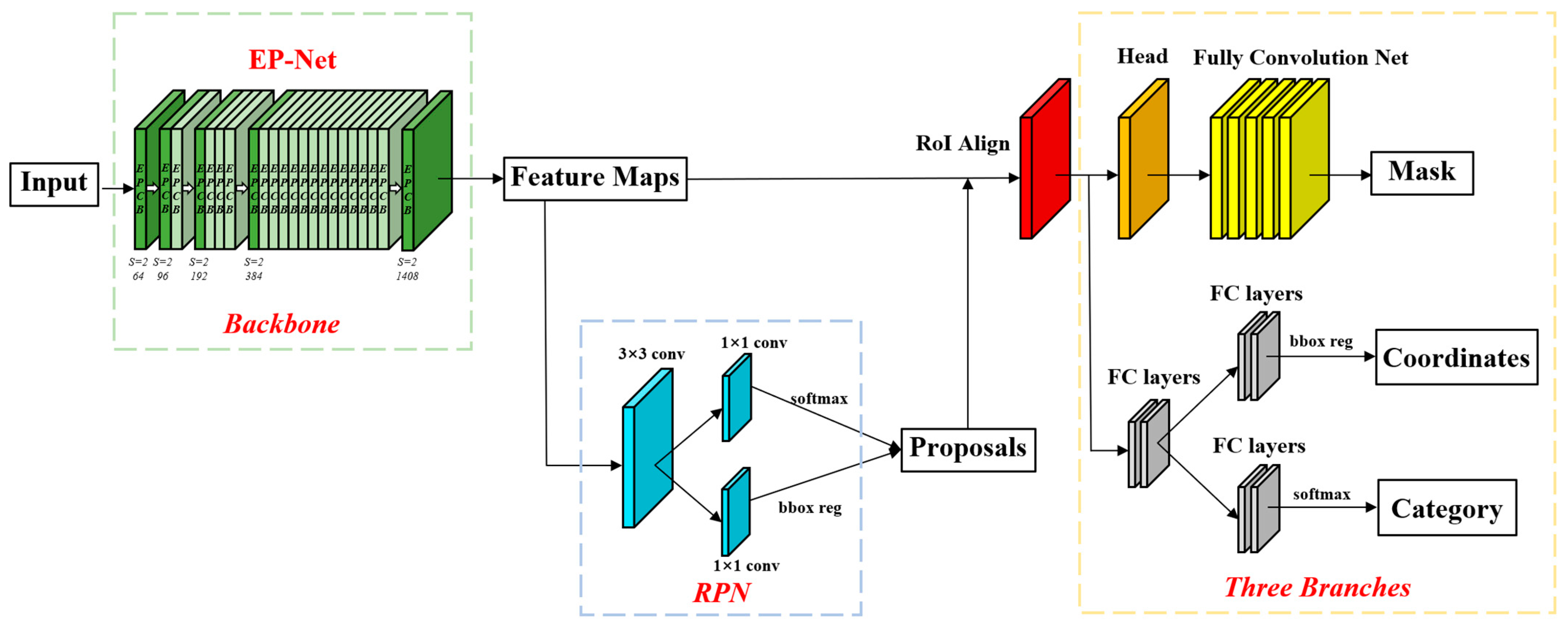
2.3. Improvement on Mask R-CNN
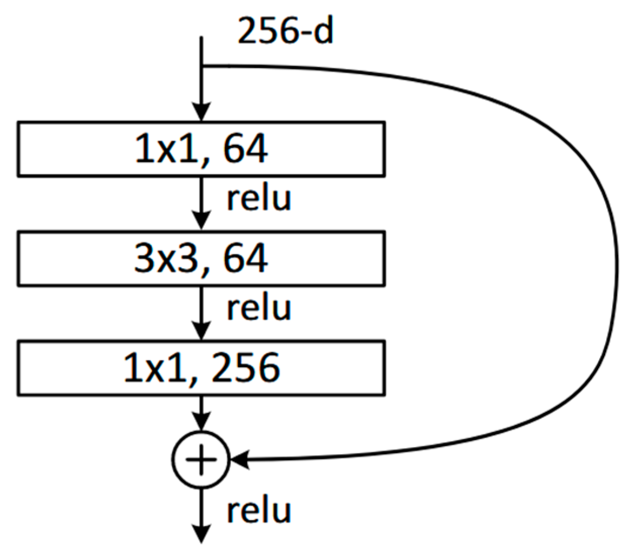
2.3.1. Edge-Prior Convolutional Block
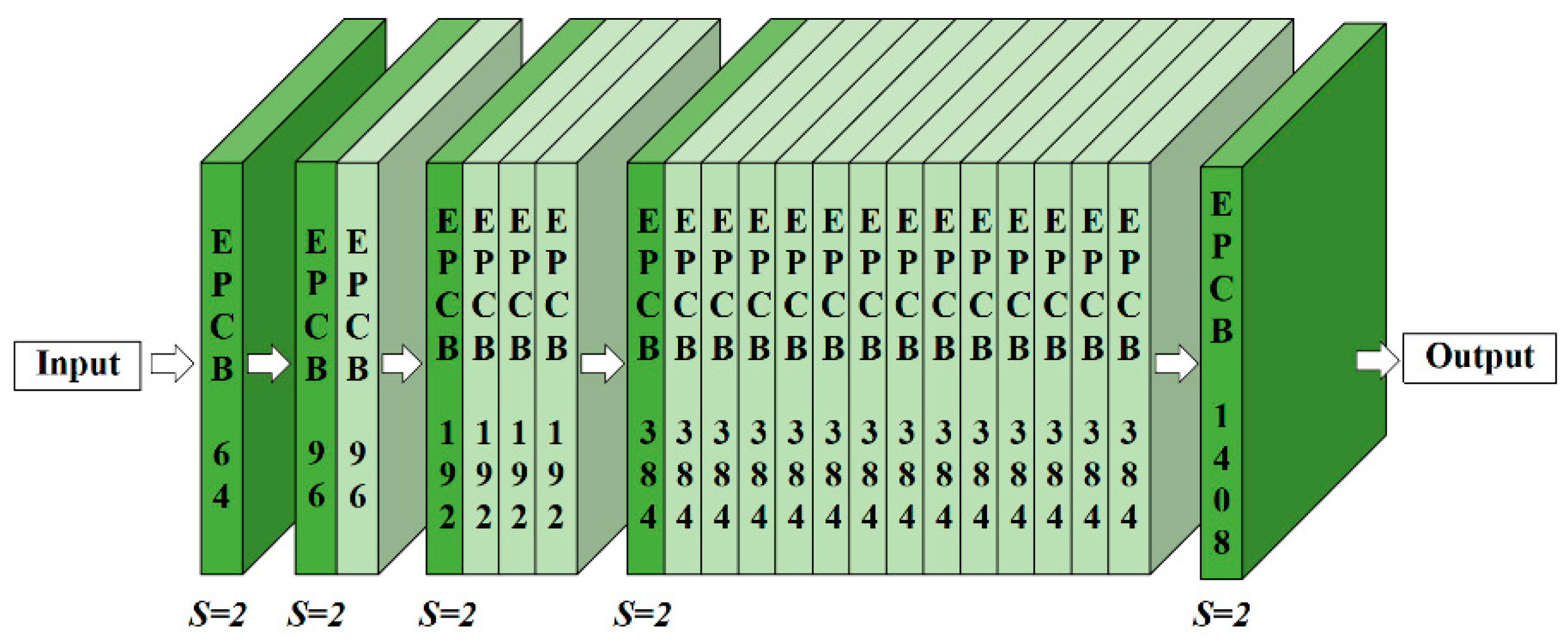
2.3.2. Edge-Prior Net
3. Experimental Data and Parameters
3.1. Experimental Data
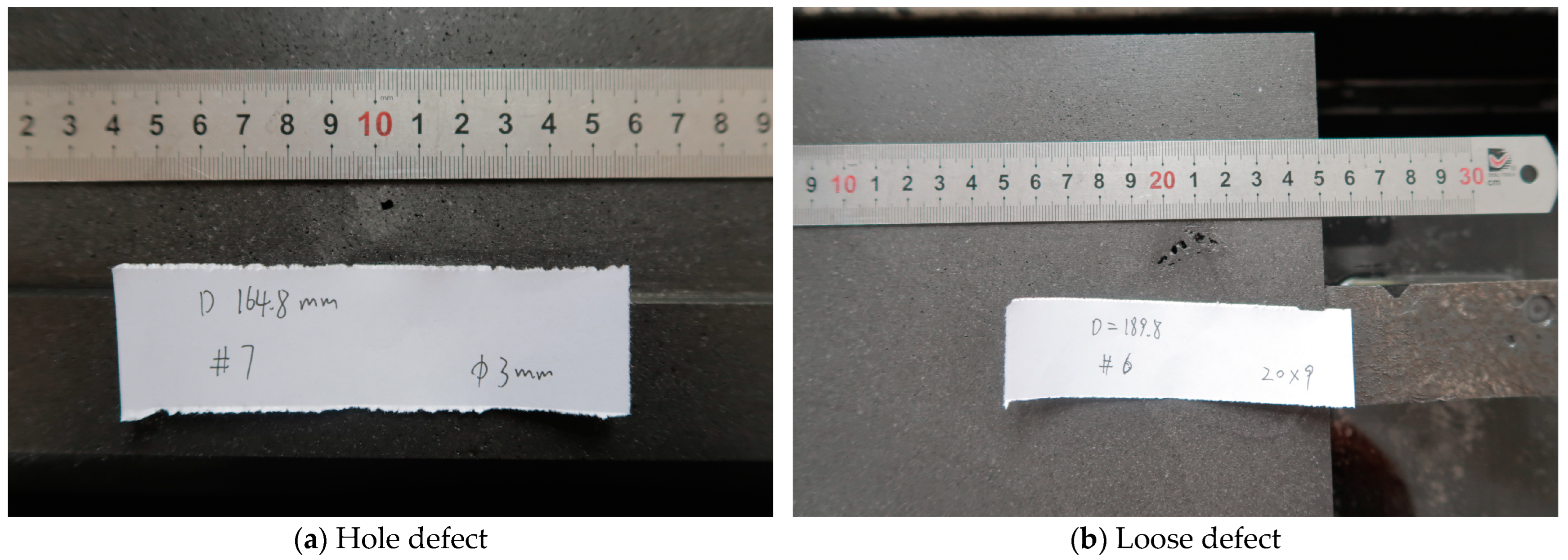
3.1.1. Actual Components Dataset
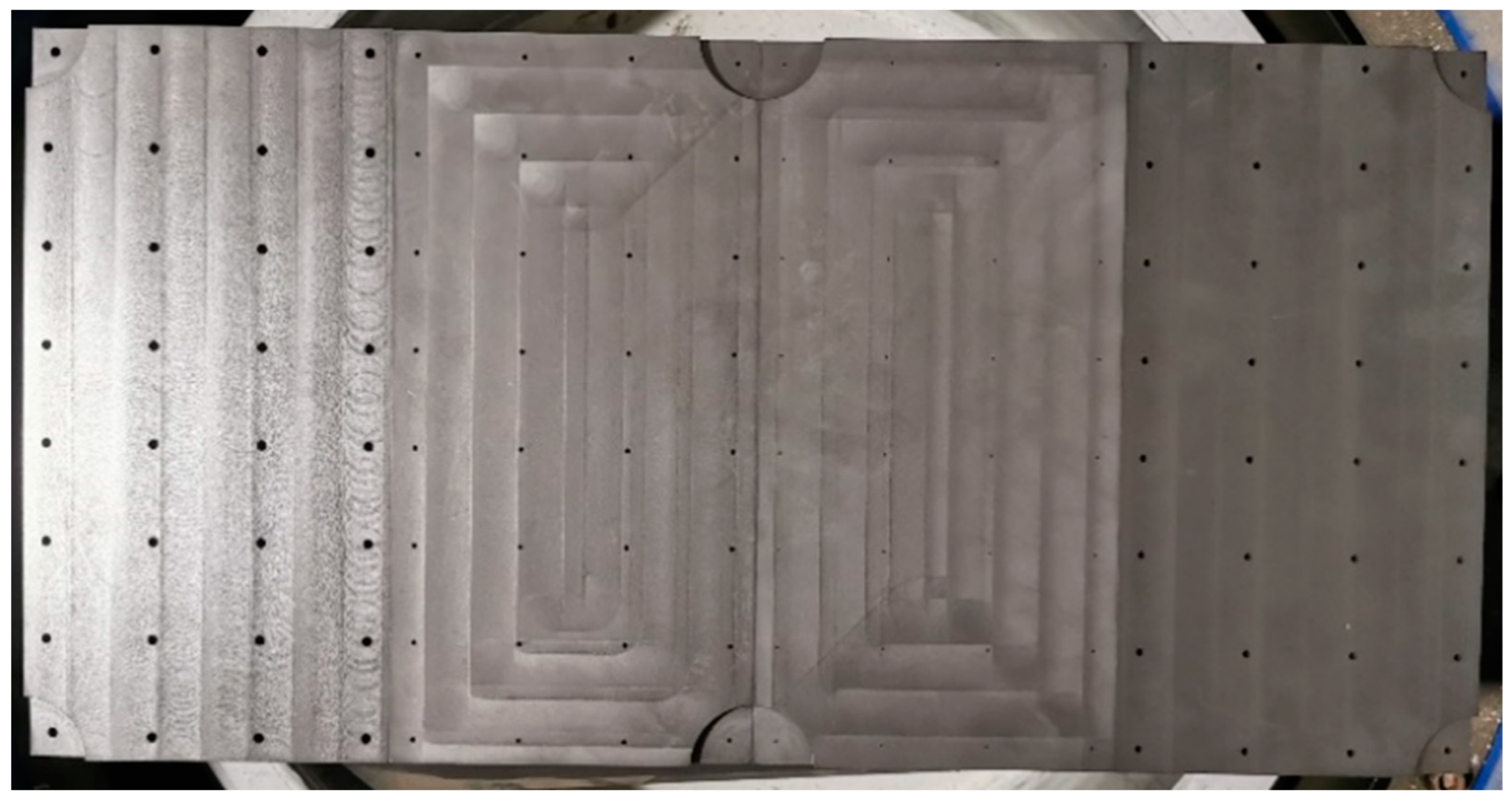
3.1.2. Test Components Dataset
3.1.3. Complete Dataset
3.2. Evaluation Metrics
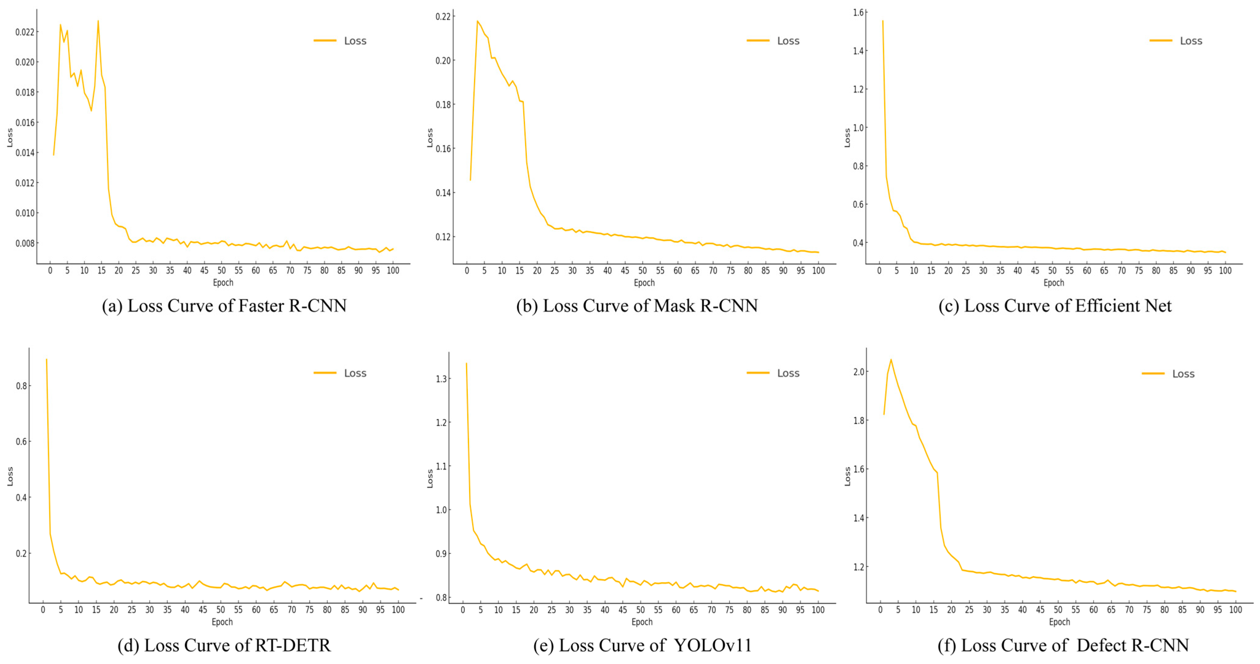
3.3. Models Training
4. Experimental Evaluation and Analysis
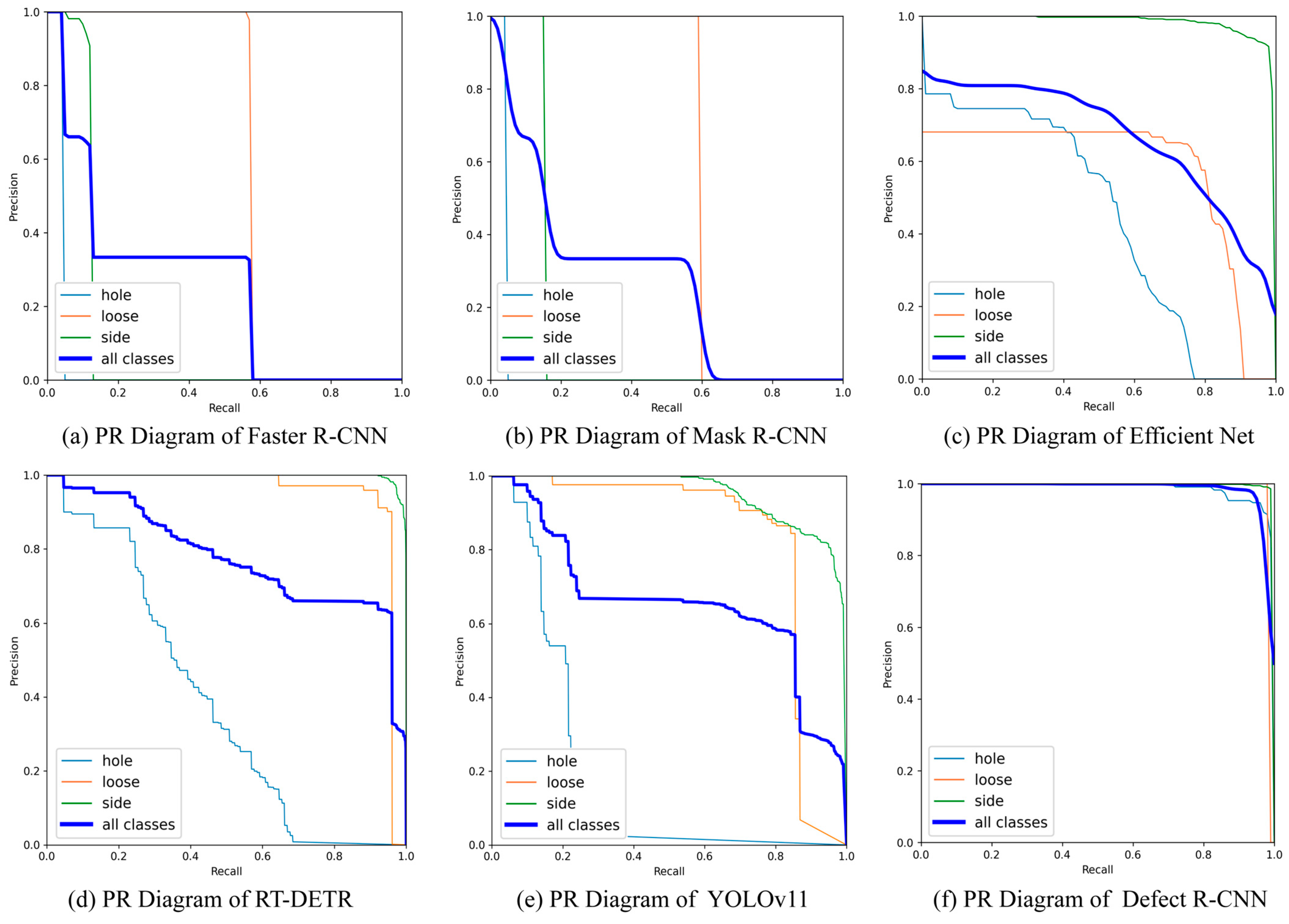
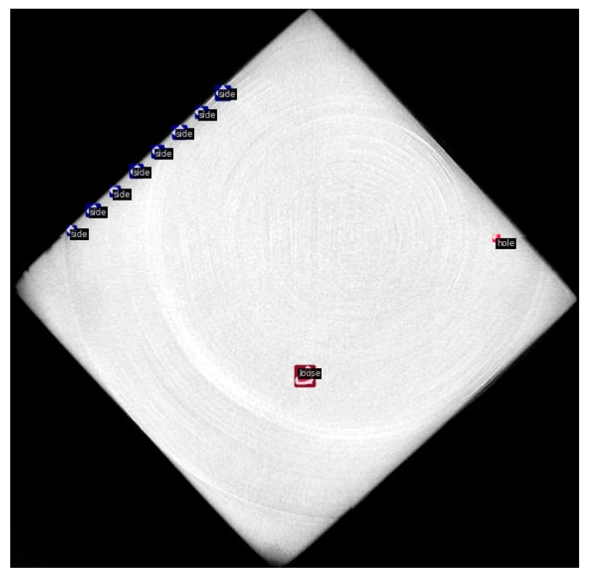
4.1. Test Results of Actual Components Dataset
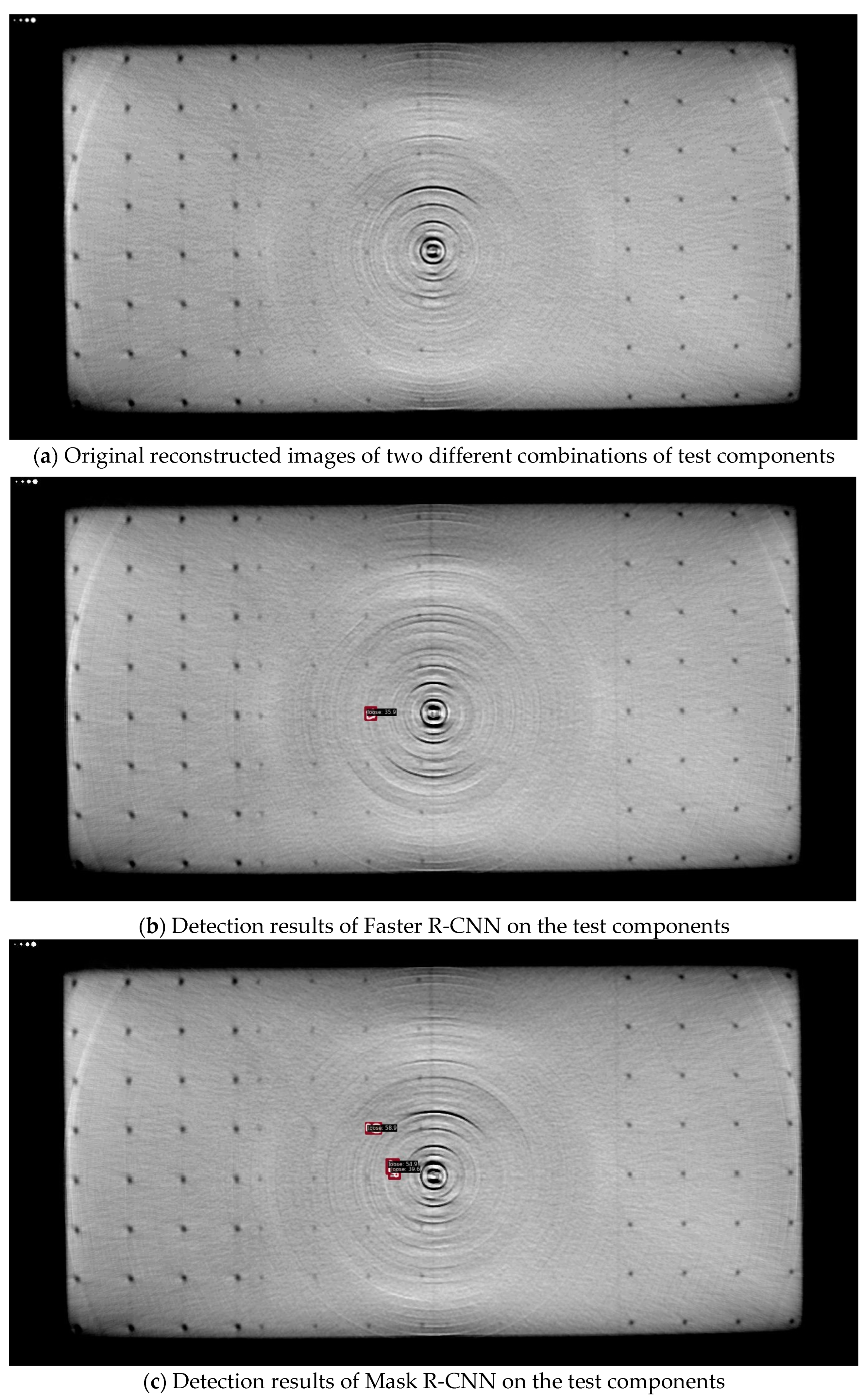
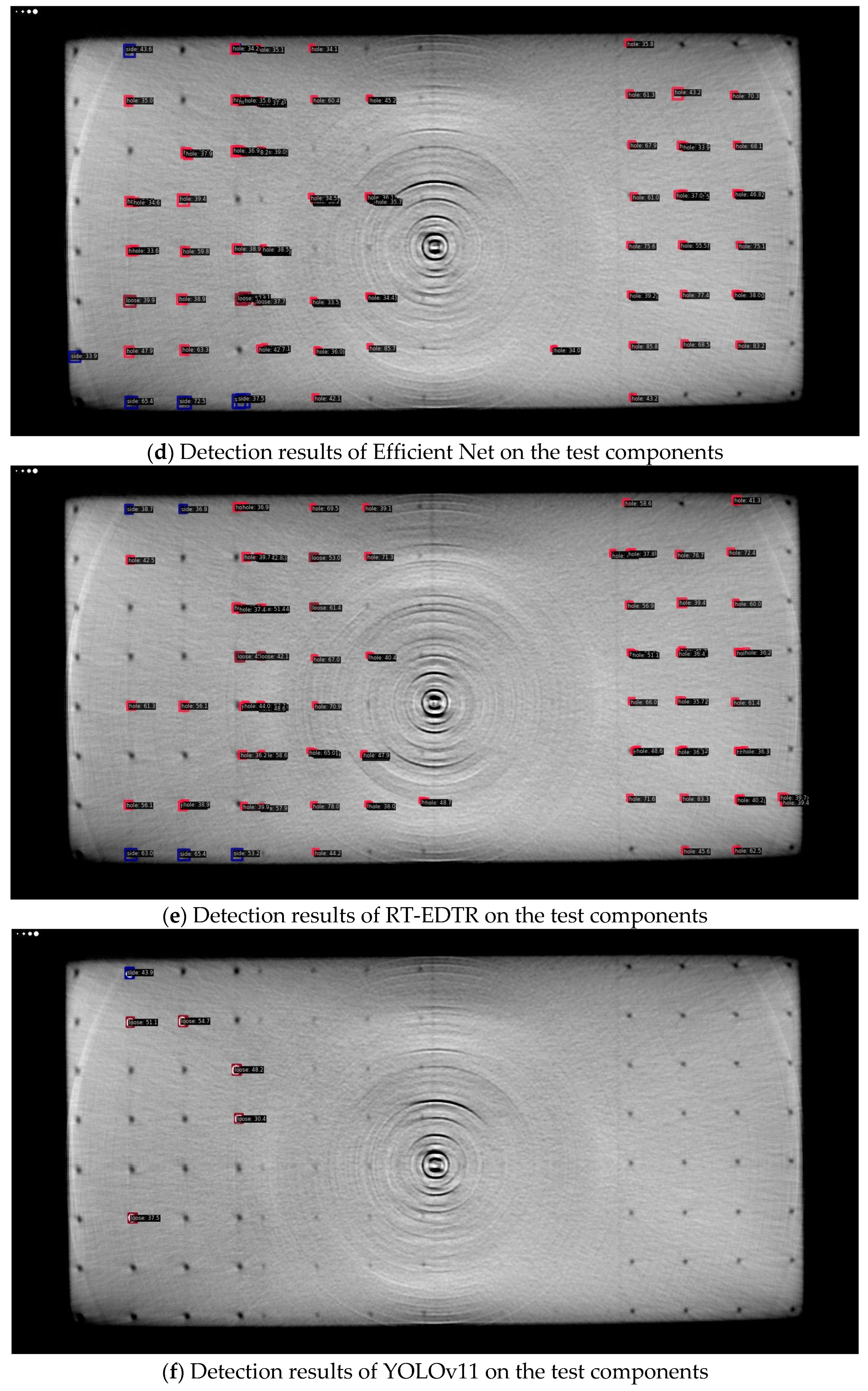
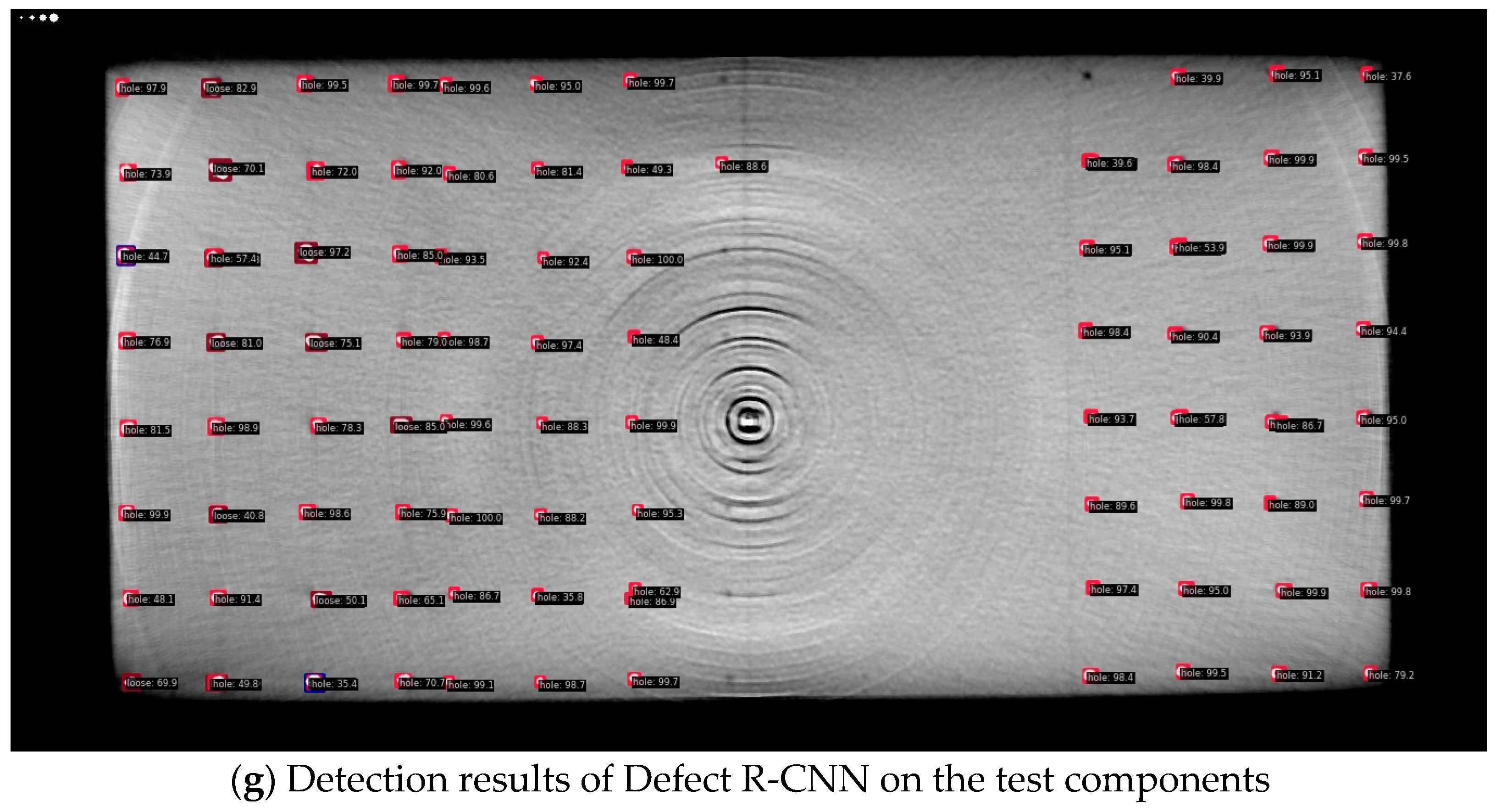
4.2. Test Results of Test Components Dataset
5. Ablation Study
6. Discussion and Conclusions
Author Contributions
Funding
Institutional Review Board Statement
Informed Consent Statement
Data Availability Statement
Conflicts of Interest
Abbreviations
| HTGR | High Temperature Gas-cooled Reactor |
| AP | Average Precision |
| mAP | mean Average Precision |
| mAP-bbox | mean Average Precision of bounding box |
| mAP-segm | mean Average Precision of segmentation mask |
| FPS | Frames Per Second |
| ET | Eddy Current Testing |
| CT | Computed Tomography |
| UT | Ultrasonic Testing |
| RT | Radiographic Testing |
| NDT | Non-destructive Testing |
| MV | Machine Vision |
| DL | Deep Learning |
| CNN | Convolutional Neural Network |
| SSD | Single Shot multibox Detector |
| YOLO | You Only Look Once |
| R-CNN | Regions with CNN features |
| Faster R-CNN | Faster Region-based Convolution Neural Network |
| Mask R-CNN | Mask Region Convolution Neural Network |
| RT-DETR | Real-Time Detection Transformer |
| DSM | Decompound-Synthesize Method |
| PSNR | Peak Signal-to-Noise Ratio |
| SSIM | Structural Similarity |
| BN | Batch Normalization |
| FLOPs | Floating Point Operations |
| GFLOPs | Giga Floating Point Operations |
| RPN | Region Proposal Network |
| MRPN | Multi-scale Region Proposal Network |
| ROI | Region of Interest |
| GAN | Generative Adversarial Network |
| IoU | Intersection over Union |
| FPN | Feature Pyramid Network |
| EPCB | Edge-Prior Convolutional Block |
| EP-Net | Edge-Prior Net |
| PR curve | precision–recall curve |
| TP | True Positive |
| TN | True Negative |
| FP | False Positive |
| FN | False Negative |
| SGD | Stochastic gradient descent |
References
- Sun, J.; Li, Z.; Li, C. Progress of Establishing the China-Indonesia Joint Laboratory on HTGR. Nucl. Eng. Des. 2022, 397, 111959. [Google Scholar] [CrossRef]
- Zeng, T.; Fu, J.; Cong, P.; Liu, X.; Xu, G.; Sun, Y. Research on Ring Artifact Reduction Method for CT Images of Nuclear Graphite Components. J. X-Ray Sci. Technol. 2025, 33, 317–324. [Google Scholar] [CrossRef]
- Johns, S.; Yoder, T.; Chinnathambi, K.; Ubic, R.; Windes, W.E. Microstructural Changes in Nuclear Graphite Induced by Thermal Annealing. Mater. Charact. 2022, 194, 112423. [Google Scholar] [CrossRef]
- Zhang, X.; Deng, Y.; Yan, P.; Zhang, C.; Pan, B. 3D Analysis of Crack Propagation in Nuclear Graphite Using DVC Coupled with Finite Element Analysis. Eng. Fract. Mech. 2024, 309, 110415. [Google Scholar] [CrossRef]
- Thomas, M.; Oh, H.; Schoell, R.; House, S.; Crespillo, M.; Hattar, K.; Windes, W.; Haque, A. Dynamic Deformation in Nuclear Graphite and Underlying Mechanisms. Materials 2024, 17, 4530. [Google Scholar] [CrossRef]
- Lu, J.; Liu, X.; Miao, J.; Wu, Z. Study on Irradiation Light Output Stability of PB-HTGR Pebble Flow CT Detector. At. Energy Sci. Technol. 2018, 52, 1685–1690. [Google Scholar] [CrossRef]
- Xiong, D.; Tsang, D.; Song, J. An Insight into Annealing Mechanism of Graphitized Structures after Irradiation. Radiat. Phys. Chem. 2024, 225, 112137. [Google Scholar] [CrossRef]
- Wang, W.; Wang, P.; Zhang, H.; Chen, X.; Wang, G.; Lu, Y.; Chen, M.; Liu, H.; Li, J. A Real-Time Defect Detection Strategy for Additive Manufacturing Processes Based on Deep Learning and Machine Vision Technologies. Micromachines 2023, 15, 28. [Google Scholar] [CrossRef] [PubMed]
- Lu, M.; Chen, C.-L. Detection and Classification of Bearing Surface Defects Based on Machine Vision. Appl. Sci. 2021, 11, 1825. [Google Scholar] [CrossRef]
- Profili, A.; Magherini, R.; Servi, M.; Spezia, F.; Gemmiti, D.; Volpe, Y. Machine Vision System for Automatic Defect Detection of Ultrasound Probes. Int. J. Adv. Manuf. Technol. 2024, 135, 3421–3435. [Google Scholar] [CrossRef]
- Tao, X.; Gao, H.; Wu, Q.; He, C.; Zhang, L.; Zhao, Y. Detection of Defects in Adhesive Coating Based on Machine Vision. IEEE Sens. J. 2024, 24, 5172–5185. [Google Scholar] [CrossRef]
- Yang, L. Fiber Optic Connector End-Face Defect Detection Based on Machine Vision. Opt. Fiber Technol. 2025, 91, 104158. [Google Scholar] [CrossRef]
- Wang, X.; D’Avella, S.; Liang, Z.; Zhang, B.; Wu, J.; Zscherpel, U.; Tripicchio, P.; Yu, X. On the Effect of the Attention Mechanism for Automatic Welding Defects Detection Based on Deep Learning. Expert Syst. Appl. 2025, 268, 126386. [Google Scholar] [CrossRef]
- Chen, Y.; Ding, Y.; Zhao, F.; Zhang, E.; Wu, Z.; Shao, L. Surface Defect Detection Methods for Industrial Products: A Review. Appl. Sci. 2021, 11, 7657. [Google Scholar] [CrossRef]
- Liu, W.; Anguelov, D.; Erhan, D.; Szegedy, C.; Reed, S.; Fu, C.-Y.; Berg, A.C. SSD: Single Shot MultiBox Detector; Springer: Cham, Switzerland, 2016; Volume 9905, pp. 21–37. [Google Scholar]
- Hussain, M. YOLO-v1 to YOLO-v8, the Rise of YOLO and Its Complementary Nature toward Digital Manufacturing and Industrial Defect Detection. Machines 2023, 11, 677. [Google Scholar] [CrossRef]
- Girshick, R.; Donahue, J.; Darrell, T.; Malik, J. Rich Feature Hierarchies for Accurate Object Detection and Semantic Segmentation. In Proceedings of the IEEE Conference on Computer Vision and Pattern Recognition, Columbus, OH, USA, 23–28 June 2014; pp. 580–587. [Google Scholar]
- Ren, S.; He, K.; Girshick, R.; Sun, J. Faster R-CNN: Towards Real-Time Object Detection with Region Proposal Networks. IEEE Trans. Pattern Anal. Mach. Intell. 2017, 39, 1137–1149. [Google Scholar] [CrossRef]
- He, K.; Gkioxari, G.; Dollár, P.; Girshick, R. Mask R-CNN. IEEE Trans. Pattern Anal. Mach. Intell. 2020, 42, 386–397. [Google Scholar] [CrossRef]
- Xu, J.; Ren, H.; Cai, S.; Zhang, X. An Improved Faster R-CNN Algorithm for Assisted Detection of Lung Nodules. Comput. Biol. Med. 2023, 153, 106470. [Google Scholar] [CrossRef]
- Gamdha, D.; Unnikrishnakurup, S.; Rose, K.J.J.; Surekha, M.; Purushothaman, P.; Ghose, B.; Balasubramaniam, K. Automated Defect Recognition on X-Ray Radiographs of Solid Propellant Using Deep Learning Based on Convolutional Neural Networks. J. Nondestruct. Eval. 2021, 40, 18. [Google Scholar] [CrossRef]
- Huang, C.; Zhou, Y.; Xie, X. Intelligent Diagnosis of Concrete Defects Based on Improved Mask R-CNN. Appl. Sci. 2024, 14, 4148. [Google Scholar] [CrossRef]
- Farag, R.; Upadhyay, P.; Gao, Y.; Demby, J.; Montoya, K.G.; Tousi, S.M.A.; Omotara, G.; DeSouza, G. COVID-19 Detection from Pulmonary CT Scans Using a Novel EfficientNet with Attention Mechanism. arXiv 2024, arXiv:2403.11505. [Google Scholar]
- Su, Q.; Qin, Z.; Mu, J.; Wu, H. YOLO Lung CT Disease Rapid Detection Classification with Fused Attention Mechanism; ACM: Xiamen, China, 2023; pp. 1381–1387. [Google Scholar]
- Liu, Y.; Liu, Y.; Zhang, P.; Zhang, Q.; Wang, L.; Yan, R.; Li, W.; Gui, Z. Spark Plug Defects Detection Based on Improved Faster-RCNN Algorithm. J. X-Ray Sci. Technol. 2022, 30, 709–724. [Google Scholar] [CrossRef] [PubMed]
- Revathy, G.; Kalaivani, R. Fabric Defect Detection and Classification via Deep Learning-Based Improved Mask RCNN. Signal Image Video Process. 2024, 18, 2183–2193. [Google Scholar] [CrossRef]
- Yu, T.; Chen, W.; Junfeng, G.; Poxi, H. Intelligent Detection Method of Forgings Defects Detection Based on Improved EfficientNet and Memetic Algorithm. IEEE Access 2022, 10, 79553–79563. [Google Scholar] [CrossRef]
- Liu, M.; Chen, Y.; Xie, J.; He, L.; Zhang, Y. LF-YOLO: A Lighter and Faster YOLO for Weld Defect Detection of X-Ray Image. IEEE Sens. J. 2023, 23, 7430–7439. [Google Scholar] [CrossRef]
- Liu, Y.; Cao, Y.; Sun, Y. Research on Rail Defect Recognition Method Based on Improved RT-DETR Model. In Proceedings of the 2024 5th International Conference on Computer Engineering and Application (ICCEA), Hangzhou, China, 12–14 April 2024; pp. 1464–1468. [Google Scholar]
- Zhao, L.; Wang, T.; Chen, Y.; Zhang, X.; Tang, H.; Lin, F.; Li, C.; Li, Q.; Tan, T.; Kang, D.; et al. A Novel Framework for Segmentation of Small Targets in Medical Images. Sci. Rep. 2025, 15, 9924. [Google Scholar] [CrossRef]
- Yada, N.; Kuroda, H.; Kawamura, T.; Fukuda, M.; Miyahara, Y.; Yoshizako, T.; Kaji, Y. Improvement of Image Quality for Small Lesion Sizes in 18F-FDG Prone Breast Silicon Photomultiplier-Based PET/CT Imaging. Asia Ocean. J. Nucl. Med. Biol. 2025, 13, 77. [Google Scholar] [CrossRef]
- Zhang, F.; Wang, Q.; Fan, E.; Lu, N.; Chen, D.; Jiang, H.; Yu, Y. Enhancing Non-Small Cell Lung Cancer Tumor Segmentation with a Novel Two-Step Deep Learning Approach. J. Radiat. Res. Appl. Sci. 2024, 17, 100775. [Google Scholar] [CrossRef]
- He, K.; Zhang, X.; Ren, S.; Sun, J. Deep Residual Learning for Image Recognition. In Proceedings of the IEEE Conference on Computer Vision and Pattern Recognition, Las Vegas, NV, USA, 27–30 June 2016; pp. 770–778. [Google Scholar]
- Torralba, A.; Russell, B.C.; Yuen, J. LabelMe: Online Image Annotation and Applications. Proc. IEEE 2010, 98, 1467–1484. [Google Scholar] [CrossRef]
- Fu, J.; Liu, R.; Zeng, T.; Cong, P.; Liu, X.; Sun, Y. A Study on CT Detection Image Generation Based on Decompound Synthesize Method. J. X-Ray Sci. Technol. 2025, 33, 72–85. [Google Scholar] [CrossRef]
- Tan, M.; Le, Q.V. EfficientNet: Rethinking Model Scaling for Convolutional Neural Networks. In Proceedings of the 36th International Conference on Machine Learning, Long Beach, CA, USA, 10–15 June 2019; Volume 97, pp. 6105–6114. [Google Scholar]
- Zhao, Y.; Lv, W.; Xu, S.; Wei, J.; Wang, G.; Dang, Q.; Liu, Y.; Chen, J. DETRs Beat YOLOs on Real-Time Object Detection. In Proceedings of the 2024 IEEE/CVF Conference on Computer Vision and Pattern Recognition (CVPR), Seattle, WA, USA, 17–21 June 2024; pp. 16965–16974. [Google Scholar]
- Khanam, R.; Hussain, M. YOLOv11: An Overview of the Key Architectural Enhancements. arXiv 2024, arXiv:2410.17725. [Google Scholar]
- Chen, K.; Wang, J.; Pang, J.; Cao, Y.; Xiong, Y.; Li, X.; Sun, S.; Feng, W.; Liu, Z.; Xu, J.; et al. MMDetection: Open MMLab Detection Toolbox and Benchmark. arXiv 2019, arXiv:1906.07155. [Google Scholar]
- Lin, T.-Y.; Maire, M.; Belongie, S.; Hays, J.; Perona, P.; Ramanan, D.; Dollár, P.; Zitnick, C.L. Microsoft COCO: Common Objects in Context. In Proceedings of the Computer Vision—ECCV 2014, Zurich, Switzerland, 6–12 September 2014; Fleet, D., Pajdla, T., Schiele, B., Tuytelaars, T., Eds.; Springer International Publishing: Cham, Switzerland, 2014; pp. 740–755. [Google Scholar]


| Module | Params (M) | Parameters Proportion | FLOPs (GFLOPs) | Computation Proportion |
|---|---|---|---|---|
| ResNet50 | 16.88 | 50.38% | 265.34 | 38.51% |
| FPN | 1.51 | 4.50% | 195.76 | 28.41% |
| RPN | 0.60 | 1.79% | 139.66 | 20.27% |
| ROI Head | 14.52 | 43.33% | 88.21 | 12.81% |
| Total | 33.51 | 100.00% | 688.97 | 100.00% |
| Parameters | Training Dataset | Test Dataset | ||||
|---|---|---|---|---|---|---|
| Actual Component | Synthetic Data Made by DSM | Total | Actual Component | Test Component | Total | |
| Number of images | 500 | 1500 | 2000 | 100 | 750 | 850 |
| Image resolution | 1536 × 1536 | 1536 × 1536 | 1536 × 1536 | 1536 × 1536 | 1360 × 760 | — |
| Number of hole defect | 205 | 6729 | 6934 | 104 | 36383 | 36487 |
| Number of loose defect | 113 | 2201 | 2314 | 48 | — | 48 |
| Number of side defect | 615 | 992 | 1607 | 184 | — | 184 |
| Faster R-CNN | Mask R-CNN | Efficient Net | RT-DETR | YOLOv11 | Defect R-CNN | |
|---|---|---|---|---|---|---|
| mAP-bbox | 0.373 | 0.415 | 0.664 | 0.776 | 0.655 | 0.983 |
| AP-bbox-50-hole | 0.048 | 0.05 | 0.442 | 0.383 | 0.187 | 0.98 |
| AP-bbox-50-loose | 0.645 | 0.67 | 0.574 | 0.953 | 0.829 | 0.98 |
| AP-bbox-50-side | 0.426 | 0.526 | 0.977 | 0.993 | 0.949 | 0.988 |
| mAP-segm | — | 0.297 | 0.411 | — | 0.381 | 0.956 |
| AP-segm-50-hole | — | 0.05 | 0.0544 | — | 0.0456 | 0.9 |
| AP-segm-50-loose | — | 0.604 | 0.675 | — | 0.663 | 0.98 |
| AP-segm-50-side | — | 0.237 | 0.503 | — | 0.433 | 0.988 |
| FPS | 68.4 | 53.5 | 100.6 | 111.8 | 91.1 | 76.2 |
| Mask R-CNN | +EPCB | +EP-Net | Defect R-CNN | |
|---|---|---|---|---|
| mAP-bbox | 0.592 | 0.774 | 0.985 | 0.986 |
| AP-bbox-50-hole | 0.05 | 0.397 | 0.98 | 0.98 |
| AP-bbox-50-loose | 0.651 | 0.982 | 0.989 | 0.989 |
| AP-bbox-50-side | 0.538 | 0.987 | 0.988 | 0.989 |
| mAP-segm | 0.313 | 0.787 | 0.961 | 0.979 |
| AP-segm-50-hole | 0.05 | 0.397 | 0.913 | 0.969 |
| AP-segm-50-loose | 0.642 | 0.978 | 0.98 | 0.98 |
| AP-segm-50-side | 0.249 | 0.987 | 0.989 | 0.989 |
| FPS | 51.91 | 50.97 | 50.96 | 78.85 |
Disclaimer/Publisher’s Note: The statements, opinions and data contained in all publications are solely those of the individual author(s) and contributor(s) and not of MDPI and/or the editor(s). MDPI and/or the editor(s) disclaim responsibility for any injury to people or property resulting from any ideas, methods, instructions or products referred to in the content. |
© 2025 by the authors. Licensee MDPI, Basel, Switzerland. This article is an open access article distributed under the terms and conditions of the Creative Commons Attribution (CC BY) license (https://creativecommons.org/licenses/by/4.0/).
Share and Cite
Jiang, Z.; Fu, J.; Zeng, T.; Liu, R.; Cong, P.; Miao, J.; Sun, Y. Defect R-CNN: A Novel High-Precision Method for CT Image Defect Detection. Appl. Sci. 2025, 15, 4825. https://doi.org/10.3390/app15094825
Jiang Z, Fu J, Zeng T, Liu R, Cong P, Miao J, Sun Y. Defect R-CNN: A Novel High-Precision Method for CT Image Defect Detection. Applied Sciences. 2025; 15(9):4825. https://doi.org/10.3390/app15094825
Chicago/Turabian StyleJiang, Zirou, Jintao Fu, Tianchen Zeng, Renjie Liu, Peng Cong, Jichen Miao, and Yuewen Sun. 2025. "Defect R-CNN: A Novel High-Precision Method for CT Image Defect Detection" Applied Sciences 15, no. 9: 4825. https://doi.org/10.3390/app15094825
APA StyleJiang, Z., Fu, J., Zeng, T., Liu, R., Cong, P., Miao, J., & Sun, Y. (2025). Defect R-CNN: A Novel High-Precision Method for CT Image Defect Detection. Applied Sciences, 15(9), 4825. https://doi.org/10.3390/app15094825