Abstract
Characterizing the coastal wave environment, typically composed of wind-driven waves and boat wakes, and its interaction with built infrastructure is essential for planning sustainable and resilient shoreline development and protection. Objectively identifying and measuring non-stationary wave features, particularly boat wakes, in longer data records remains a challenge. A wave gauge array of four pressure sensors was deployed for several weeks in the northernmost section of urbanized Tampa Bay, FL, a sheltered, shallow (mean depth 1.2 m) region with frequent recreational small-boat activity. New methods for analyzing these measurements were explored. The array had a square geometry, allowing the calculation of directional spectra. Most prior studies of boat wakes could only examine amplitude spectra. A nearby seawall was found to be a significant source of wave reflection. Additionally, a novel empirical method for identifying wakes, distinguishing them from wind-driven waves, and providing an estimate of their duration and amplitude was developed. The method was found to reliably identify most primary wakes but not reflected wakes. Reflected boat wakes were identified manually, and only during times of relatively high water levels when the shoreline in front of the seawall was flooded.
1. Introduction
Boat-driven waves [1,2], generally known as “wakes” or “wash”, along with wind-driven waves are primary mechanisms of coastal erosion and bank retreat [3,4,5,6,7]. Seawalls are a common form of hardening built to protect shorelines from wave energies, but these reflect waves back into the environment and can generate scouring at their base [8,9]. In regions of frequent boat activity, wakes can potentially compromise the stability of protective structures, such as seawalls, levees and reventments [10,11], archaeological sites [11], and other nearshore structures. Wakes can also create a broad range of negative impacts on aquatic ecosystems. For example, wakes can enhance sediment resuspension and turbidity, inundate nesting shorebirds, and displace invertebrates, fish eggs, and larvae [12,13,14]. Understanding wake properties is therefore essential for resiliency planning of many coastal regions [15]. Boat wake form, amplitude, and propagation vary with vessel shape, speed, and size, along with water depth and dimensions of the water body [16,17,18]. The multi-variate dependence of wake properties has motivated the use of in situ measurements of wakes in order to determine wake characteristics in specific locations and vessel traffic patterns. We present results from a field study of wind waves and recreational boat wakes in a sheltered sub-embayment of Tampa Bay, FL, that employed novel methods for assessing wave reflection and identifying and measuring ship wakes.
Ship wakes are wave packets generated by objects moving on or near the water surface. They form their distinctive ‘V’-shape due to the dispersion properties of surface gravity waves, as first derived by Kelvin [19] for a point source in deep, open water, and explored by others for more general cases [20,21,22,23]. Wakes travel at the group velocity . Boat wakes are typically created when a vessel travels above a minimum value of the length-based Froude number [24,25,26], where and are the ship length and speed, respectively, and = 9.8 m s−2 is the gravitational acceleration. Wake amplitude (and associated wave drag) increases with , reaching a peak near the “hull speed” at 0.4 [27,28], limiting the speed of displacement vessels. These wakes typically have two primary components. The first is the dispersive “divergent” component whose signal increases in frequency when measured at a fixed point (“chirp”). The second is the relatively narrow-banded “transverse” wave.
Some moderate sized and many small personal water craft can operate in planing or semiplaning mode, and can travel above hull speed by exploiting hydrodynamic lift forces [25,29]. The transverse component and the total wake height of (semi)planing boats generally decrease as their speed increases above hull speed. The angle from the shipline at which the wake travels is 35° in the Kelvin solution and increases for ≥ 0.4 [22,30,31,32]. In shallow water, the depth-based Froude number, , where is the water depth, also plays a determining role in the wake angle and propagation.
Many earlier studies of boat wakes were restricted to conditions where wakes dominated the wave field, either due to limited wind fetch or relatively high amplitude wakes, in order to better isolate the wake signals. In the more general case, windowed Fourier and wavelet techniques have been widely applied to provide a visualization of the time–frequency behavior of dispersive wake packets that often allows for wakes to be identified and distinguished from wind-generated waves [33,34,35,36]. However, in those studies wakes were generally identified by manual inspection of the wavelet amplitude, a potentially laborious procedure when working with large data sets. One novel aspect of this study was the development of a new wavelet-based objective method for wake identification that yielded the wake start time, duration, and chirp rate.
Additionally, most previous publications examining measurements of boat wakes used a single sensor, from which only amplitude and frequency could be computed, or a group of linearly arranged sensors, from which propagation along the array line could also be found. Directional wave information would aid in determining wave origins, attribution to their impacts, and help the development of any management response [37,38], as well as wave–infrastructure interactions, including reflection. Here, a geometric (square) array of pressure sensors was used, allowing for the calculation of directional spectra, differentiation between incoming and reflected wakes, and improved understanding of the wake dynamics and behaviors. Geometric arrays of sensors have been used to examine open ocean and coastal directional spectra e.g., [39,40], but have not been widely applied to wakes. This manuscript presents one of the first studies of wake reflection, though the presence of reflected wakes have been inferred in previous studies [41].
The new approaches presented can also support the design and implementation of living shorelines [42,43,44,45], which are of increasing interest as alternatives to seawalls and other armored coastal structures built to protect shorelines from erosion due to wave action. The design of most living shorelines are often guided by numerical models that may not fully represent the range of conditions in a specific location [46,47,48]. Directional wave gauges can provide additional information on the wave environment useful for planning such projects and for measuring their effectiveness at wave absorption post-installation by measuring changes in shoreline reflectivity. This study was part of the pre-installation phase of living shoreline planned for installation at the study site.
The following section describes the study site, the design of the wave gauge, and the methodologies used in the analysis, particularly the spectral methods employed, including directional and wavelet methods, and the algorithm for objective identification of wakes. Section 3 details the types of wave signatures found, the effectiveness of the identification algorithm, and the presence of wake reflections. Section 4 presents a Discussion of the results.
2. Materials and Methods
2.1. Study Site
Safety Harbor (Figure 1a) is a microtidal region with dimensions about 2 km by 3 km and connects to Old Tampa Bay on its roughly 1 km wide southern boundary. It is bounded to its west by Philippe Park, which is comprised of 122 acres located along the western shores of the harbor. The park was acquired by the local government in 1948 and contains significant archaeological sites. There is a concrete seawall along the western bank of the harbor to protect an adjacent walkway and park land area from erosion primarily from wave action and storm surge. The seawall directly south of the gauge extends about 45 m to the southeast before turning southward. Nearshore water depth is nominally 1 m, but near the seawall, the bottom shoals is often exposed at low tide. It was therefore reasonable to assume there was little boat traffic between the gauge and seawall during this study. Central Safety Harbor has a nominal water depth of ~2–3 m but reaches up to 5 m depth (Figure 1b). Wind fetch from most directions was limited, but the southern boundary of Safety Harbor is open to Tampa Bay with fetch about 10 times that of Safety Harbor.
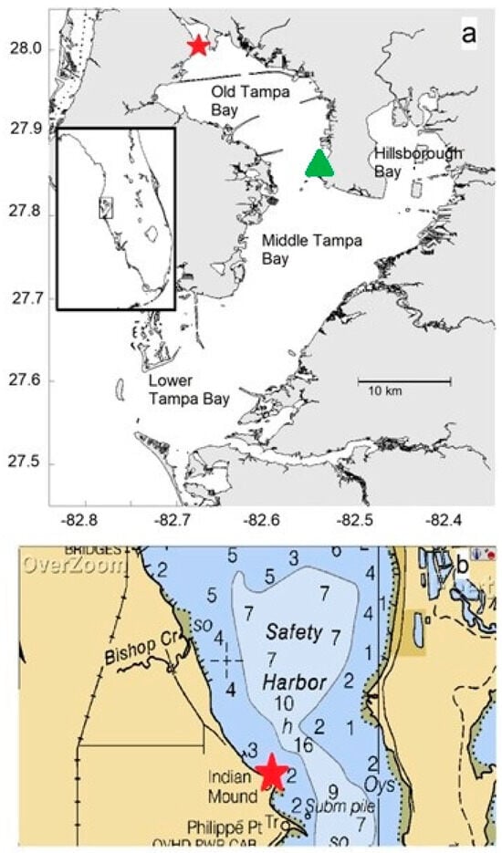
Figure 1.
Location of the wave gauge (star). (a) Tampa Bay major segments and location on the Florida coast (inset). NOAA gauge 8726607 location (green). (b) Navigation chart near deployment. Depth units are feet.
Relevant historical environmental conditions near the sensor site based on federal long-term monitoring data were assessed by [49]. They examined tidal datums, storm surge elevations, historic wind records, and critical fetch lengths. Using a nearby tide gauge (NOAA #8726738), they calculated the tidal range of about 0.85 m. Winds at St. Petersburg and Tampa airports over 48 years showed widely varying wind direction, with almost all speeds being less than 12 m/s. Winds from the northeast were about twice as common as any other direction. The winds during this deployment were generally light, with a mean scalar speed of 2.8 m/s, only exceeding 5 m/s during about 9% of the deployment (Figure 2a). Winds were again generally from the north and northeast (Figure 2b).
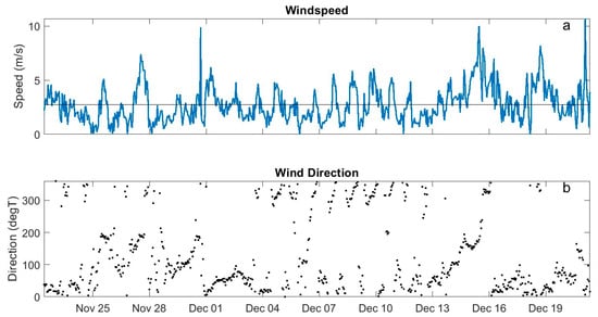
Figure 2.
Hourly winds from NOAA gauge 8726607 in Old Tampa Bay (Figure 1). (a) wind speed (blue) and mean scalar speed (black); (b) wind direction (degrees True).
2.2. Sensor Array
Four RBR Coda 3 pressure gauges were mounted on a 2 m × 2 m square transportable platform, along with an RBR Concerto 3 data logger (Figure 3) that synchronized and recorded all measurements. The sensors were set to measure pressure (sensor number ), at a sampling frequency = 4 Hz, sufficient to sample most surface gravity waves. The array frame was constructed from 1” diameter PVC piping. The mean water depth at the sensor site was about 1.2 m. The array was deployed about 62 m offshore from the seawall.
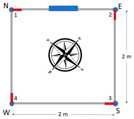
Figure 3.
Schematic of sensor array. Numbered sensors are red, and the logger is blue. Geographic orientation during deployment is indicated.
The dimension of 2 m was selected to provide a phase difference of the measured waves across the array. Typical wave periods in Tampa Bay are about 2 s [50]. Site inspection prior to gauge deployment found this value to be a nominal lower bound to the wave period. The wavelength of these fast waves can be estimated using the deep water approximation , about 3 m. The 4 Hz sampling rate of the array therefore yielded about 7 points per cycle. Larger waves with longer periods had more points per cycle. Longer periods would have larger wavelengths until they transition to intermediate or shallow water conditions, where , and increasing sample points per cycle.
During deployment, the array was fixed about 2 cm off the bottom using screw mounts to secure their position. Changes in water level induced by waves induced changes in bottom pressure, which were measured by the sensors. The sensors selected for this project had an accuracy ≤ 3 × 10⁻⁴ dbar, or around 0.3 mm, and were factory-calibrated. There was no method to compensate for variations in the bottom terrain (nominally 1–10 cm). These small variations only impacted the absolute depths, not measures of the tidal and wave signals that were the focus of this study. The gauge and logger were activated before they were deployed and were stopped when they were disassembled after recovery and cleaning. Pressure data for all sensors were downloaded using the RBR Ruskin v2.19.1 software package. The deployment examined here was from 22 November 2022 to 21 December 2022.
Recreational boats that compromised almost all the traffic in Safety Harbor do not broadcast through the Automatic Identification System [38], so their size, position, and velocity could not be determined. Therefore, ten controlled boat passes were performed over a period of one hour, and their resulting wakes were measured by the array. On 29 November 2022, personnel from Pinellas County made 10 boat passes in the vicinity of the wave gauge (Table 1). Three position readings were taken during each pass along with the boat speed. The boat was a Parker XL1800 (Cleveland, OH, USA), 5.2 m long, with a 115 HP motor. Pass ‘A’ in Table 1 was a skiff driven by a private citizen of indeterminate length. No other boats were operating in Safety Harbor in the vicinity of the gauge during this time. Wind speeds, as measured by a NOAA gauge located about 18 km from the study site, the day before and during this exercise were <4 m/s (Figure 2), so wind-waves were weak compared to the boat generated waves. This was not always true during the entire deployment.

Table 1.
Supervised boat passes. For each pass: pass number, start of each pass, the approximate speed of the pass, the estimated Froude numbers dimensionless depth, and maximum wake amplitude from (4) are shown. The pass at 9:40 was a vessel not associated with this study.
2.3. Data Processing
The times before and after deployment when the gauges were still active were easily identified by inspection and removed from the pressure signals . The pressure measurements were converted to water depth , where = 2010 kg/m3 was the nominal density of the estuarine water at the study site. The relative depth was used to represent the tidal stage and was found to have implications for wake dynamics (below).
2.3.1. Filtering
The depth values were high-pass filtered using a 30 min passband with a steepness of 0.85. The cutoff frequency was selected to be at least one order of magnitude from the periods of the waves being considered (1–10 s) and the highest frequency major tidal component (semidiurnal, ~12 h). Using a 30-min cutoff therefore minimized filtering effects on the wave frequencies and effectively suppressed the tidal frequencies. To minimize numerical artifacts in the filtering process, before filtering the data were demeaned and padded with zeroes so the total number of points was 2n. The filtered signal was back-transformed into real space to obtain the high-pass signal . The initial and final 2 h were removed from the analysis to eliminate residual end-point effects. Wave amplitudes were identified as positive peaks in with at least a 20 s interval between them. The average and maximum wave heights were computed. Wave amplitude was the deviation from the mean and was ½ the wave height.
2.3.2. Spectral Analysis
The Fourier spectrum of an infinite time series is
where is the spectral frequency. The power spectrum was then , for > 0. The finite time spectrum was computed using the Fast Fourier Transform (FFT). Filtering of was accomplished using [51,52].
In this study, the time domain was limited to the period of measurement, and was such that it formed either a high-pass or bandpass filter.
The DIrectional WAve SPectra Toolbox (DIWASP, Version 1.4) [53,54] was used to transform the set of four into a directional spectral power function , where was direction. Note that and were discrete values representing the spectra within bin sizes of and , respectively. The total wave energy from a particular direction was determined by summing the energy within all frequency bins. Measures of the incoming and reflected wave energies were calculated by summing over the relevant directional ranges. See [55,56,57] for some additional applications of DIWASP.
2.3.3. Wavelet Analysis
Continuous wavelet analysis [58,59,60] of an infinite time series is defined as the convolution of a function with a collection of translations and dilations of a zero-mean “mother” wavelet function . Wavelets were used to decompose the signals into the time–frequency domain [61,62]. The decomposition expanded the one-dimensional, real data into a two-dimensional, complex domain
This allowed for separation of amplitude and phase signal elements. Here, is a continuous function with compact support, and * indicates complex conjugate. The parameter is the ‘scale’ or dilation parameter whose inverse can often be directly related to a Fourier frequency [63], so the transform can be equivalently examined in time–frequency space . The Morse wavelet [64,65] was used in this analysis because it is a continuous, oscillatory complex function whose Fourier transform [65] exists only on the positive real axis. Morse wavelets provide good correlation with the type of signals generated by both boat wakes and wind-driven waves. Normalization by in (2) scales the magnitude of such that spectral components are more easily compared [66]. This is in contrast to the more common scaling of [67] that suppresses the amplitude of high-frequency signals relative to lower-frequency signals. The continuous transform is not orthonormal, but it is invertible. In this case,
where
and is the angular frequency. The limits on Equation (4) are known as the admissibility condition. The window is a localized time–frequency filter suitable for highlighting specific signals but can also be configured as a spectral bandpass by removing dependence on , or as a full inverse by setting = 1. Equation (4) was used below with to isolate the wake signal from the wind-generated wave field and calculate wake amplitude and duration.
Boat wakes are often distinguishable from wind driven waves under time–frequency decomposition [33,35,41]. Wakes from small boats, such as those examined in this study, are coherent wave packets with nominal periods of several seconds, and duration of several minutes. When measured by a stationary instrument, their waveform shifts from low frequency to high frequency over time [41], which is reflected in their amplitude as a distributed, arching maxima. Such a changing frequency structure is commonly referred to as a “chirp” [68]. In contrast, wind-driven coastal waves (below) more closely resemble a random process at high frequencies.
2.3.4. Wake Identification
An objective method for identifying wakes was developed based on the chirp signal of the wakes as represented in wavelet space [69]. A family of parabolic curves was generated such that time ( coordinate for curve at frequency was
These were segments of horizontal parabolas with vertices at () and terminations at (), where was the wake duration and = 5 s. The latter being equivalent to the resolution of the duration measure and was much less than the typical wake duration. Quadratics were used to approximate the dispersion of wakes emanating from shiplines of varying orientation and distance from the gauge and poorly known propagation paths over varying bathymetry. For each time, these K-curves were convolved with the masked wavelet amplitude . The convolution took the form of a summation over each K-line
was the number of frequencies included in the integration, from = 0.1 Hz to = 0.6 Hz, the nominal range of the observed wakes. This choice reduced overlap with the typically higher-frequency wind waves. Mask values were equal to one everywhere but were set to zero for < −8, an empirical value corresponding to the nominal amplitude found by examining during time periods of low wind and no boat traffic. This value is likely dependent on and the local wave environment. Applying the mask decreased noise in . The K-lines were designed to detect divergent wakes typically generated when > 0.4 and > 1.
The parameter ranged from 1 to 120, yielding K-curves from 5 sec to 10 min long. A range of values was used since the duration of any particular wake signal was unknown. Wake duration varies with distance traveled by the wake due to wave dispersion—the further the wake travels the longer the signal and the lower its amplitude [70]. The that maximized for each time was selected to create a time series . Long-term background values were calculated using a 20-min Hanning window and removed . This rectification reduced the likelihood of a small peak being falsely identified due to high background values, as was often found during periods of high wind. Peaks of sufficient indicated high correlation between the curves and the wavelet amplitude, and were identified as wakes with duration . This convolutional approach was less computationally intensive then other methods of wake identification when considering unknown shape and duration, such as application of machine learning [71], ridge regression [72], and manual confirmation [35]. For brevity this method will be referred to as AWD (Algorithm for Wake Detection) through the rest of this article.
To summarize, the sequential steps of the AWD are:
- Set-up
- Compute masked ;
- Determine wake frequency range defined by [;
- Find the nominal minimum frequency () of wind waves;
- the wake duration resolution ;
- Select range of such that maximum matches or exceeds longest expected wake duration;
- Define generic set of K-curve array positions for .
- Calculate M(t)
- Integrate over each K-curve starting at the initial , yielding ;
- Determine the that maximizes ;
- Define and at this maximal value of ;
- Repeat for all times of interest.
- Remove background M (rectification)
- Smooth using window much larger than maximum wake duration to generate ;
- Calculate .
- Wake Detection
- Find times of local maxima of ;
- For each , partition into and ;
- Calculate the means and of the two segments;
- If then delete this from the set of wakes, otherwise retain.
Testing of the estimated duration and start times derived from the AWD indicated that the results were insensitive to noise for signal-to-noise ratios (SNRs) above about 0.1 (Appendix A). That is, the AWD was reliable until the noise level significantly exceeded the wake signals. The mean SNR for the identified wakes was 14.8, indicating the results obtained from the AWD were unlikely to have been contaminated by background signals.
3. Results
Wave properties were examined in three ways. The first involved study of common wave forms found in the sensor data. The second involved wakes generated by supervised boat passes, allowing for clear associations between the recorded wakes with known boat activity. The third assessed bulk wave properties over the 29-day deployment.
3.1. Wave Forms
Examination of presented two primary types of signals in that occurred both individually and in combination. The first type was found in a narrow-band (nominally 0.5–1 Hz) with modulating amplitude that produced a ‘keyboard’-like structure in (Figure 4a,c). Directional analysis indicated multiple sources from which these waves were propagating (Figure 5a). This type of signal was associated with wind-driven waves and persisted for minutes to many hours.
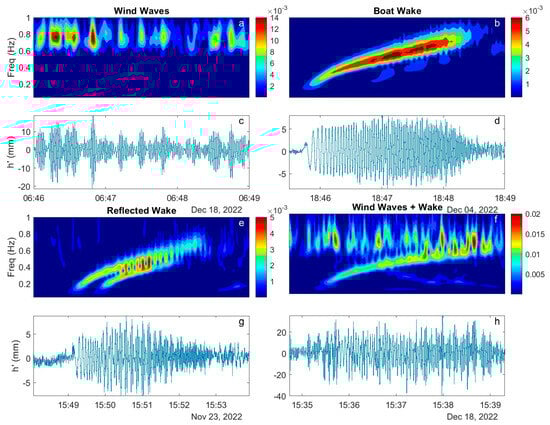
Figure 4.
Common wave types (a,c) wind waves; (b,d) boat wake; (e,g) double (reflected) wake; (f,h) wind wave and wake. Shown are (a,b,e,f) wavelet amplitude and (c,d,g,h) corresponding wave signal h′.
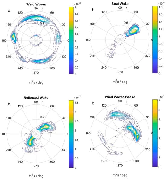
Figure 5.
Directional power spectra from the four-sensor array during the time periods in Figure 4. (a) wind waves; (b) boat wake; (c) double (reflected) wake; (d) wind wave and wake.
The second type (Figure 4b,d) was a smooth wake packet that progressed from lower to higher frequencies (roughly 0.15 to 0.8 Hz) and displayed a temporally narrow chirp structure in wavelet space. These were associated with boat wakes and generally persisted for 1–10 min. Many wake signals were found to be isolated, with one direction of origin (Figure 5b), indicating direct propagation from the boat’s travel line to the location of the gauge. The general lack of spectral overlap of wind waves and boat wakes at frequencies below ~0.5 Hz was important for the development of the AWD in Section 2.3.4. Figure 5b also provided a test of the angular resolution. A single wake packet can be presumed to have originated from a unique direction. The angular resolution of the DIWASP 1.4 software is an adjustable parameter and, in this case, was set to 30°. This resolution was reasonable for the purposes of this study (Figure 5b). The practical resolution will depend on the array configuration, sampling rate, and signal frequency.
A third type of signal was found composed of two overlapping wakes (Figure 4e,g). The in these cases generally showed a beating pattern found when two signals of similar frequency are summed. In this case, the frequency of both wakes ( and ) increased with time, yielding an increasingly rapid carrier wave of period and slowing envelope with period . The difference in arrival times at the gauge of these wakes were finite and typically between 30 and 90 s. The delay was found to be reasonably estimated for a boat traveling parallel to a seawall over a flat bottom (Figure 6), the travel time for the reflected wave to reach the gauge would be , where was the angle of propagation relative to the shipline, and is the distance from the seawall to the gauge. Similarly, the travel time directly from the boat to the gauge would be . The difference in travel time was then , where is the celerity of the wave. This yielded a delay time of 30 s between arrival of the primary wake and the reflected wake, assuming 1.3 m of water, = 62 m, and an angle of (from the Kelvin solution), comparable to the measured values. Direction of boat travel, angle of propagation, and dependence of on depth are likely the most significant sources of uncertainty in this estimate.
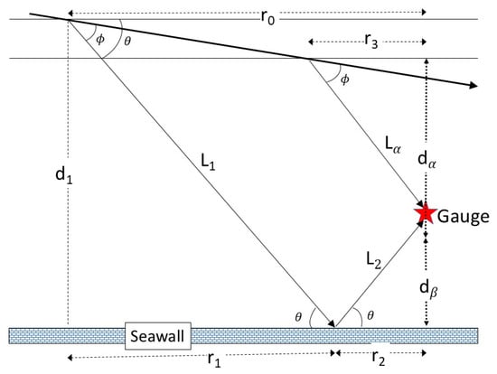
Figure 6.
Paths of boat wakes generated by boat passing (heavy arrow) at an angle with respect to straight seawall. The angle of propagation relative to the shipline is . The gauge-intersecting paths of reflected wake (L1 + L2) and directly impacting wake (Lα) are indicated.
The assumption that the secondary wake was a reflection was further supported by the directional spectrum of this signal, which showed two directions from which the signals propagated (e.g., Figure 5c). One direction was from the deeper region of Safety Harbor, where most boat activity occurs; the second direction was from the seawall. The DIWASP package could not be used to separately verify the different directions of the two wave packets as directional spectra for short (~1 min) time series were sensitive to small changes in length of the input data. Reflected wakes were further documented in the supervised boat passes (below).
The fourth type of signal was a combination of wind-driven waves and wakes. These tended to yield more irregular signals (Figure 4f,h) as the modulating wind waves interacted with the frequency change of the wake. In this case, the two wave types overlapped at moderate to higher frequencies (0.5–0.9 Hz). The directional spectrum was more broadly distributed than the previous boat wake example (Figure 5d).
3.2. Supervised Boat Passes
Most of the wakes recorded in this study were undocumented, with no information on the boat size, speed, direction, or location that generated the wave signals. Supervised boat passes allowed a direct association between recorded wakes at a particular time and vessel activity, as well as testing and calibration of the AWD. Ten passes over a variety of paths, speeds, and distances from the gauge were conducted over 1 h using a single boat (Figure 7, Table 1). The odd-numbered passes were from the west or northwest, and the even-numbered were from the east or southeast. The mean water depth at the gauge changed from 1.28 m to 1.16 m from the first to final transit. Passes 5, 7, and 8 were farthest from the gauge, about 330 m, and 2, 4, and 10 were the closest, about 5, 5, and 1 m, respectively. Passes 7–10 were the fastest, and 6 the slowest. Values of ranged from 0.4 to about 2, and ranged from 0.8 to 4.2, assuming a mean depth of 1.2 m. The water depth over each path varied, with several being between 2 and 3 m deep, but remained > 1.
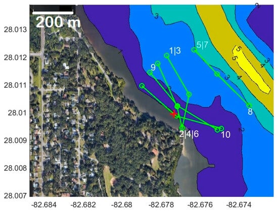
Figure 7.
Boat passes 29 November 2022 (green) near the wave gauge (red). Start, middle, and end boat positions indicated with circles. Pass number is indicated near the starting point. The gauge position was (82.677326° W, 28.009944° N). Mean bathymetry (contours) from [73] was adjusted to match the mean gauge depth. See Table 1 for boat speed.
The start of the generated wakes at the gauge were all identifiable as rapid increases in the amplitude of , followed by a decline over many oscillations to near background levels (Figure 8). The signal strength of each wake varied, and their maxima were taken as representative of the wake amplitude. All wakes were composed of a single wave form, except for wakes 4 and 10, both of which generated two distinct wave packets separated by about 15 and 30 s, respectively. The largest wake was from pass 1, with an amplitude of 51 mm. This wake also had a waveform distinct from the others, likely due to the boat motor being trimmed up, pushing the bow higher, the stern lower, and increasing the effective and . All other passes were with vertical trim. The second largest was from pass 4 at 32 mm. The weakest wakes were from passes 7–9, with amplitudes 8–9.5 mm (Table 1). These low-amplitude wakes were also the highest , except for pass 10 that had but generated a higher wake amplitude, 23 mm. This was due to the proximity of the travel line to the gauge, a minimum of ~1 m, so there was little time for the initial disturbance to disperse.
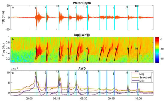
Figure 8.
Wakes from supervised boat passes (Figure 7) on 29 November 2022: (a) high-passed water level () from sensor 1 (orange). Objectively identified wake times (cyan); (b) the natural logarithm of the wavelet amplitude. K-lines of identified primary wakes (solid black) are indicated; (c) Wake-detection function (, orange), smoothed (, yellow), and rectified (, purple). The wake between pass 7 and 8 was not part of this study. See Table 1 for details of each pass.
One other boat traveled through the study area between passes 7 and 8. This was identified as a Carolina skiff about 5 m in length on a path such that its wake was recorded by the gauge. No other boats were in the vicinity of the gauge during this time. The AWD correctly identified the presence of 11 wakes in the supervised period (Figure 8a). The times of maximum and their associated -lines showed a close correspondence with the primary wakes revealed in (Figure 8b). However, AWD did not detect the reflected signals. This was due to the peak of the reflections mixing with those of the primary wake, creating a relatively weak, one-sided peak that was below the detection threshold. Setting the detection threshold low enough to find the reflections resulted in many false positives.
Some wakes showed similar temporal development (Figure 9). Many wakes had secondary (reflected) wakes as indicated by a second dispersive feature following the first in , and by their directional spectra (Figure 10). In some cases (e.g., passes 7 and 8), the lower frequencies of the reflected wake were attenuated compared to the primary wake. The reason for this was unclear. The of wakes 2 and 6 were similar, but their spectral evolution was different (Figure 9), with wake 6 having a single, non-dispersive structure indicative of the transverse wake common for low-Froude number wakes, whereas wake 2 was composed of two dispersive wakes.
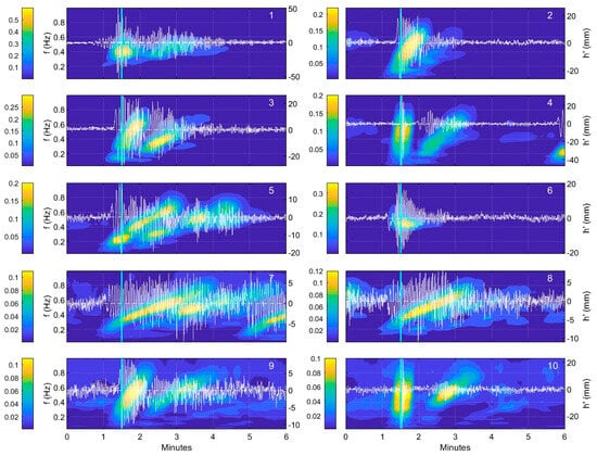
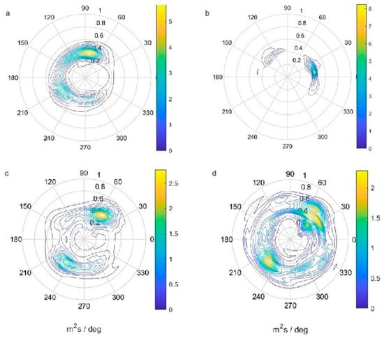
Figure 10.
Directional power spectrum for supervised boat passes (a) 1; (b) 6; (c) 7; and (d) 10. Units are ×10−6. See Table 1 for details of each pass.
The durations of the primary wakes as determined by the AWD were an underestimate of the complete wake signal (Figure 11, Table 2). One reason for this was the cutoff of the K-lines at intermediate frequency to avoid sampling the higher, primarily wind-driven frequencies, terminating the fit even when the wake contained higher frequencies. A more significant reason in relation to determining the total duration was the presence of secondary (reflected) wakes, which overlapped the original wake signal. The reflections started later and tended to have longer duration than the primary wake (Table 2). This was the result of dispersion as the reflected wake traveled a longer distance than the wake arriving directly from the boat (Figure 6). An exception was pass 6, which had no reflected wake (at the gauge site). However, there was a close linear relation between the duration determined from AWD () and the duration determined directly from plots of the wavelet amplitude (). The AWD value was about one-half of that measured (Figure 11), with about a 2% uncertainty (Figure 11). Exceptions to this were the wakes from passes 1 and 6, which were outside the dynamical regimes for which AWD was designed. The total duration from , denoted , was defined as the difference between the end of the secondary wake and the beginning of the primary wake. had a similar rate of dependence on , but with an uncertainty around 15%. These findings were used for estimating the total time of boat wakes over the deployment (below).
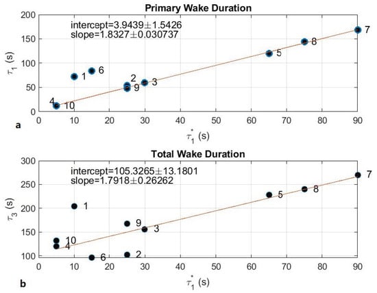
Figure 11.
Duration of primary supervised wakes from AWD () vs. measured duration of (a) primary wake () from (dots); (b) total wake () from (dots). Linear fit to all but Pass 1 and 6 is show (red) with the slopes and intercepts indicated.
3.3. Bulk Properties
The AWD detected wakes by identifying peaks in the function. False positives were found in cases of high wind-wave activity. These were characterized by values of along the lower-frequency portion of the maximum K-line less than about 0.178 Hz being much lower than the high-frequency portion, indicating that the K-line was sampling wind waves. Instances with mean values in the lower frequency portion were < 1/5 of the mean in the higher-frequency portion were eliminated. After this quality control procedure, the AWD yielded 383 wakes, with a mean duration of 5.3 min.
Vessel operations are generally determined by vessel type and function. Recreational boaters prefer to be on the water during times of high visibility. Most of the AWD-identified wakes were found during daylight hours (Figure 12), consistent with boat activity being comprised of recreational vessels. Wakes outside these times may have been law enforcement or from boats engaged in night fishing, but there was insufficient information to confirm this conjecture.
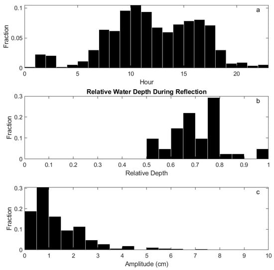
Figure 12.
Statistics derived from AWD. (a) The hour of objectively identified wakes; (b) relative water depth () during reflection identified subjectively; (c) amplitude of all objectively identified wakes.
As noted above, many wakes had no reflection. The occurrence of reflection was found to be tidally controlled. The water depth computed from determined the reflectivity of the seawall. All reflections, identified manually by the presence of a second dispersive wake in immediately following an AWD-identified wake, occurred for 0.5 (Figure 12). No reflected waves were identified during relatively shallow time periods. This was likely due to the shoaling of the shoreline which is exposed during low tide and submerged during high tide. In future studies, the effective reflectivity of the seawall might be estimated by examining the ratio of the reflected wave energy compared to that of the incoming wave.
The maximum amplitudes of each wake were determined using (4) with defined as a polygon around each AWD-identified wake. The beginning of each polygon was 1 min prior to the identified time and the end determined using the relation between and in the previous section. The polygon sides were curved to match the maximum K-line associated with each wake. The mean amplitude of the identified wakes was 1.1 cm with a median of 0.8 cm. This was larger than the mean amplitude of the over the entire deployment (0.2 cm), but this low overall value was likely due to the sheltered location resulting in only intermittent significant wind-generated waves.
Wave energy over the entire deployment was largely from two general directions, the northeast and southwest (Figure 13). The former was the direction of relatively open water, and the latter the direction of the seawall from which they were likely reflected. The largest spectral peak was from the northeast near 6 Hz and was about twice that of the peak of the reflected waves, which also peaked just above 6 Hz. The total energy from the direction of the seawall comprised ~23% of the total energy. This was determined by integrating the power spectrum (Figure 13) over all frequencies and directions and comparing that to the integrated energy over all frequencies but limited to the directional range of the wall (170°–270°) determined by the directional analysis.
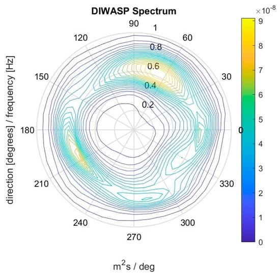
Figure 13.
Directional power spectrum from full deployment.
4. Discussion and Conclusions
A square array of pressure gauges was deployed in an urbanized estuary at a sheltered location with frequent small-boat traffic. The geometry of the array allowed for calculation of directional spectra, a capability that can be useful for coastal planning science and management. For example, directional spectra can help back-trace the origin of wave signals. Potential sources include open ocean or local open waters, structures, such as seawalls or flood control barriers, shipping channels, ports or marinas, or even specific vessels. Distinguishing these disparate sources is useful in adaptation and resilience planning. The directional spectrum can provide information to sort multiple sources by direction, and rank by frequency and intensity. Including additional parameters of time or weather conditions can help develop a dynamic picture of the wave environment, such as separating incoming swell from local wind waves or quantifying how wake propagation and potential reflection from hard boundaries is impacted by the tidal level. While directional wave studies have been common for many years, these have typically involved intermittent sampling bursts, separated by comparable periods without measurements. These limited sampling regimes were developed when battery power and data storage were at a premium but are still useful for very long-term deployments or when only gross wave statistics are needed.
The use of continuous sampling at relatively high rates (compared to the ambient waves) necessary to fully measure ship wakes, as presented here, has not been widely performed. Wake durations are generally several minutes. Interrupting their measurements would result in degraded understanding of their forms and impact. In this study, wake from the personal craft were typically 5 min in duration. Wakes from larger commercial vessels will be significantly longer due to the much larger wavelengths and wave periods generated. Continuous, extended sampling is therefore essential to capture these signals.
Such measurements help support management of coastal areas by providing quantitative measures of the wave environment and the effectiveness of any decisions or regulations such as changes to shoreline structures, vessel speed and size limitations, or coastline morphology. The study site examined here will soon have a living shoreline installed along the seawall to reduce wave impacts and enhance resilience of the region. New measurements using the same wave array at the same location are planned. Impacts of the installation on wave reflectivity (absorptivity) will be performed by computing changes to the energy spectrum from the direction of the seawall compared to the pre-installation spectrum (Figure 13). This will validate the effort associated with the project and provide information useful to future similar projects.
Measurements of wake characteristics, such as amplitude, frequency, duration, and occurrence rates, are useful for designing shoreline protective measures, as these quantities impact the wave energy and their ability to resuspend sediments. In field studies of the wave environment, detecting wakes and separating them from wind-driven wave fields can be challenging [74,75]. Separation has often been accomplished by estimating and then subtracting the nominal wind wave environment from the total signal. This typically required either a strong wake-to-wind wave signal, or a priori knowledge of approximate wake arrival time. The AWD developed here was able to identify wakes under a wide range of conditions and is robust under a range of conditions (Appendix A).
The AWD was optimized for wave forms with dispersive signals, as is commonly found originating from boats operating at a high Froude number, as well as part of more complex wakes from lower Froude number boats. The algorithm was found to be skillful in the detection of primary wakes but not reflected wakes. It would be useful to adapt the AWD to detect reflected signals. This might be accomplished through changes in detection thresholds or pre-conditioning the search using times of detected primary wakes. Experience in this study suggested a minimum of 1 min was required for a stable solution to the directional spectrum. This was consistent with a frequency resolution (, where s is signal length) around 0.03 Hz, which was sufficient to resolve the signals between 0.1 and 1 Hz. Applying the AWD to other vessel types and conditions would likely require additional adjustments to the algorithm, particularly the spectral range and perhaps the form of the K-lines. For example, larger ships generally operate at < 0.4 and produce more complex, lower-frequency wakes with multiple branches in time–frequency space. Additionally, when traveling in shallow or confined waterways these ships can sometimes generate non-dispersive solitons [76,77]. In the case of non-dispersive wakes, it might be possible to replace the K-lines with another filter, such as a simple box, in the computation of . More work is required to expand the AWD method to other Froude ranges and bathymetric conditions.
As the number and size of recreational and commercial vessels continue to increase globally, there is a corresponding growth in potentially destructive wake energy in the coastal environment. Nearshore ecosystems and human infrastructure are increasingly vulnerable to the effects of this form of energy pollution. Quantifying relevant wave characteristics is a first step for designing protective or mitigating structures needed to manage this growing concern. Application of the methods developed here can support such efforts.
Author Contributions
Author S.D.M. developed the objective methodology, conducted the data analysis, and drafted the manuscript. Author M.E.L. designed, built, and operated the wave gauge and edited the manuscript. Author S.D. helped develop the project objectives, conducted the boat pass operations, and helped edit the manuscript. All authors have read and agreed to the published version of the manuscript.
Funding
A grant from the National Fish and Wildlife Foundation (award #0318.20.68852) funded this study. Pinellas County Division of Environmental Management and Tampa Bay Estuary Program contributed to the purchase of the wave array equipment.
Data Availability Statement
Raw pressure data from each of the RBR gauges are available at https://doi.org/10.5063/F1668BMM accessed on 20 April 2025.
Acknowledgments
Pinellas County staff helped with deployment and retrieval of the monitoring equipment. Members of the Tampa Bay Estuary Program helped with project planning and data archiving.
Conflicts of Interest
The authors declare no conflict of interest.
Appendix A
To better assess the accuracy of the AWD, a synthetic test case consisting of a wake plus white noise was generated and processed through the algorithm. A noise-reduced version of the wake in Figure 4 was created by applying a bandpass filter to this data segment with cutoffs of 1 sec and 30 sec (Figure A1). The filtered data () were used as the baseline. Before filtering, the base signal was subject to 30 s cosine tapers at the endpoints, and buffered with 1 min of zeros. After filtering the buffering regions were removed.
The characteristic amplitude () of the base signal was taken as the maximum of . The start time () and durations (, as described in the text) of the base wake were determined using the AWD. Since and are linearly related (Figure 11), only the former duration was examined. White noise was added to the base signal , where were random numbers on the intervals [−1 1] . The amplitude of the noise varied over the interval from to . For each , 1000 independent realizations of were generated. The AWD was applied to each realization, and start times and durations () were computed. The signal to noise ratio (SNR) was quantified as , where rms() 0.577, the standard value for white noise on the given interval. Accuracy of the AWD for the duration and start times were defined as, respectively, and (Figure A2).
For SNRs greater than about 0.1, the estimated durations from the AWD were comparable to that of the base line. Below this value the estimated durations became increasingly uncertain, with relatively large standard deviations in the values estimated by the AWD. The error of the detected time of the wake deteriorated below a SNR of about 0.8, but even the highest noise levels examined only deviated from by a few seconds. The SNR for the initial case in Figure 4 was 6.1. In this case, the noise was defined as rms(). The mean SNR value for all detected wakes was 3.85.
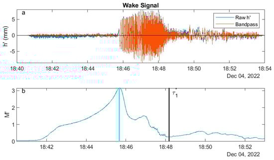
Figure A1.
(a) The raw water level (blue) and the base signal (orange); (b) from the AWD for this data segment. The AWD wake start time (cyan) and estimated durations (black) are indicated. See text for definitions.
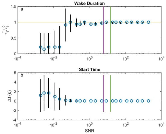
Figure A2.
Error statistics of the AWD for vs. the signal to noise ratio (SNR). Median values are indicated with ‘o’. Vertical black lines are the mean ± 1 standard deviation. The estimated SNR for the base case (green) and the average SNR for all wakes (purple). (a) The primary duration () from the AWD normalized by the value from the base case; (b) the difference in the wake initial time () from the AWD minus that of the base case ().
References
- Kirkegaard, J.; Kofoed-Hansen, H.; Elfrink, B. Wake wash of high-speed craft in coastal areas. In Coastal Engineering 1998; ASCE: Reston, VA, USA, 1998; pp. 325–337. [Google Scholar]
- Saha, G.K.; Abdullah, M.S.B.; Ashrafuzzaman, M. Wave wash and its effects in ship design and ship operation: A hydrodynamic approach to determine maximum permissible speed in a particular shallow and narrow waterway. Procedia Eng. 2017, 194, 152–159. [Google Scholar] [CrossRef]
- Almström, B.; Larson, M.; Hallin, C. Decision support tool to mitigate ship-induced erosion in non-uniform, sheltered coastal fairways. Ocean Coast. Manag. 2022, 225, 106210. [Google Scholar] [CrossRef]
- Shuster, R.; Sherman, D.J.; Lorang, M.S.; Ellis, J.T.; Hopf, F. Erosive potential of recreational boat wakes. J. Coast. Res. 2020, 95, 1279–1283. [Google Scholar] [CrossRef]
- Zhao, K.; Coco, G.; Gong, Z.; Darby, S.E.; Lanzoni, S.; Xu, F.; Zhang, K.; Townend, I. A review on bank retreat: Mechanisms, observations, and modeling. Rev. Geophys. 2022, 60, e2021RG000761. [Google Scholar] [CrossRef]
- Gemba, K.L.; Sarkar, J.; Cornuelle, B.; Durofchalk, N.C.; Sabra, K.G.; Hodgkiss, W.S.; Kuperman, W.A. Differential arrival time accuracy using ships of opportunity. J. Acoust. Soc. Am. 2017, 142, 2709. [Google Scholar] [CrossRef]
- Meyers, S.D.; Luther, M.E.; Ringuet, S.; Raulerson, G.; Sherwood, E.; Conrad, K.; Basili, G. Ship wakes and their potential shoreline impact in tampa bay. Ocean Coast. Manag. 2021, 211, 105749. [Google Scholar] [CrossRef]
- Ahmad, N.; Bihs, H.; Myrhaug, D.; Kamath, A.; Arntsen, Ø.A. Numerical modeling of breaking wave induced seawall scour. Coast. Eng. 2019, 150, 108–120. [Google Scholar] [CrossRef]
- Taylor, D.; Hall, K.; MacDonald, N. Investigations into ship induced hydrodynamics and scour in confined shipping channels. J. Coast. Res. 2007, 50, 491–496. [Google Scholar] [CrossRef]
- Bauer, B.O.; Lorang, M.S.; Sherman, D.J. Estimating boat-wake-induced levee erosion using sediment suspension measurements. J. Waterw. Port Coast. Ocean Eng. 2002, 128, 152–162. [Google Scholar] [CrossRef]
- Miller, S.E.; Ayers-Rigsby, S.; Murray, E.J.; LeFebvre, M.J.; Kangas, R.; Karim, A. Archaeology as a method and tool for resilience. Southeast Archaeol. 2024, 43, 110–122. [Google Scholar] [CrossRef]
- Gabel, F.; Lorenz, S.; Stoll, S. Effects of ship-induced waves on aquatic ecosystems. Sci. Total Environ. 2017, 601, 926–939. [Google Scholar] [CrossRef]
- Fleit, G.; Baranya, S. Acoustic measurement of ship wave–induced sediment resuspension in a large river. J. Waterw. Port Coast. Ocean Eng. 2021, 147, 04021001. [Google Scholar] [CrossRef]
- Zajicek, P.; Wolter, C. The effects of recreational and commercial navigation on fish assemblages in large rivers. Sci. Total Environ. 2019, 646, 1304–1314. [Google Scholar] [CrossRef] [PubMed]
- Bilkovic, D.M.; Mitchell, M.M.; Davis, J.; Herman, J.; Andrews, E.; King, A.; Mason, P.; Tahvildari, N.; Davis, J.; Dixon, R.L. Defining boat wake impacts on shoreline stability toward management and policy solutions. Ocean Coast. Manag. 2019, 182, 104945. [Google Scholar] [CrossRef]
- Dias, F. Ship waves and kelvin. J. Fluid Mech. 2014, 746, 1–4. [Google Scholar] [CrossRef]
- Parnell, K.E.; Soomere, T.; Zaggia, L.; Rodin, A.; Lorenzetti, G.; Rapaglia, J.; Scarpa, G.M. Ship-induced solitary riemann waves of depression in venice lagoon. Phys. Lett. A 2015, 379, 555–559. [Google Scholar] [CrossRef]
- Wu, H.; He, J.; Liang, H.; Noblesse, F. Influence of froude number and submergence depth on wave patterns. Eur. J. Mech. B/Fluids 2019, 75, 258–270. [Google Scholar] [CrossRef]
- Kelvin, L. On ship waves. Proc. Inst. Mech. Eng. 1887, 38, 409–434. [Google Scholar]
- Crawford, F.S. Elementary derivation of the wake pattern of a boat. Am. J. Phys. 1984, 52, 782–785. [Google Scholar] [CrossRef]
- Wehausen, J.V. The wave resistance of ships. In Advances in Applied Mechanics; Yih, C.-S., Ed.; Elsevier: Amsterdam, The Netherlands, 1973; Volume 13, pp. 93–245. [Google Scholar]
- Darmon, A.; Benzaquen, M.; Raphaël, E. Kelvin wake pattern at large froude numbers. J. Fluid Mech. 2013, 738, R3. [Google Scholar] [CrossRef]
- Benzaquen, M.; Darmon, A.; Raphaël, E. Wake pattern and wave resistance for anisotropic moving disturbances. Phys. Fluids 2014, 26, 092106. [Google Scholar] [CrossRef]
- Hager, W.H.; Castro-Orgaz, O. William froude and the froude number. J. Hydraul. Eng. 2016, 143, 02516005. [Google Scholar] [CrossRef]
- Watson, D.G. Practical Ship Design; Elsevier: Amsterdam, The Netherlands, 2002; Volume 1, p. 535. [Google Scholar]
- Froude, W. Experiments Upon the Effect Produced on the Wave-Making Resistance of Ships by Length of Parallel Middle Body; Institution of Naval Architects: London, UK, 1877. [Google Scholar]
- Yousefi, R.; Shafaghat, R.; Shakeri, M. Hydrodynamic analysis techniques for high-speed planing hulls. Appl. Ocean Res. 2013, 42, 105–113. [Google Scholar] [CrossRef]
- Toby, A.S. Us high speed destroyers, 1919–1942: Hull proportions. Nav. Eng. J. 1997, 109, 155–177. [Google Scholar] [CrossRef]
- Papanikolaou, A. Ship Design: Methodologies of Preliminary Design; Springer: Berlin/Heidelberg, Germany, 2014; p. 627. [Google Scholar]
- Pethiyagoda, R.; McCue, S.W.; Moroney, T.J. Wake angle for surface gravity waves on a finite depth fluid. Phys. Fluids 2015, 27, 061701. [Google Scholar] [CrossRef]
- Zhu, Y.; He, J.; Wu, H.; Li, W.; Noblesse, F. Basic models of farfield ship waves in shallow water. J. Ocean Eng. Sci. 2018, 3, 109–126. [Google Scholar] [CrossRef]
- Rabaud, M.; Moisy, F. Ship wakes: Kelvin or mach angle? Phys. Rev. Lett. 2013, 110, 214503. [Google Scholar] [CrossRef]
- Didenkulova, I.; Sheremet, A.; Torsvik, T.; Soomere, T. Characteristic properties of different vessel wake signals. J. Coast. Res. 2013, 65, 213–218. [Google Scholar] [CrossRef]
- Pethiyagoda, R.; Moroney, T.J.; Macfarlane, G.J.; Binns, J.R.; McCue, S.W. Time-frequency analysis of ship wave patterns in shallow water: Modelling and experiments. Ocean Eng. 2018, 158, 123–131. [Google Scholar] [CrossRef]
- Torsvik, T.; Soomere, T.; Didenkulova, I.; Sheremet, A. Identification of ship wake structures by a time–frequency method. J. Fluid Mech. 2015, 765, 229–251. [Google Scholar] [CrossRef]
- Robbins, A.; Thomas, G.; Amin, W.; MacFarlane, G.; Renildon, M.; Dand, I. Vessel wave wake characterisation using wavelet analysis. Int. J. Marit. Eng. Trans. R. Inst. Nav. Archit. Part A 2013, 155, 59–66. [Google Scholar] [CrossRef]
- Valbuena, S.A.; Schladow, S.G.; Bombardelli, F.A. Boat effects on lake water clarity and the efficacy of a no-wake zone policy. Lake Reserv. Manag. 2025, 41, 16–33. [Google Scholar] [CrossRef]
- Scully, B.M.; Young, D.L.; Ross, J.E. Mining marine vessel ais data to inform coastal structure management. J. Waterw. Port Coast. Ocean Eng. 2020, 146, 04019042. [Google Scholar] [CrossRef]
- Ewans, K.C. Observations of the directional spectrum of fetch-limited waves. J. Phys. Oceanogr. 1998, 28, 495–512. [Google Scholar] [CrossRef]
- Ranasinghe, D.P.L.; Kumara, I.G.I.K.; Caldera, H.P.G.M.; Engiliyage, N.L. Adaptation of Directional Wave Measurement in 3d Physical Model to Eliminate the Reflection Component in Uni-Directional Waves. In Proceedings of the 28th International Ocean and Polar Engineering Conference, Sapporo, Japan, 10–15 June 2018. [Google Scholar]
- Sheremet, A.; Gravois, U.; Tian, M. Boat-wake statistics at jensen beach, florida. J. Waterw. Port Coast. Ocean Eng. 2013, 139, 286–294. [Google Scholar] [CrossRef]
- Leatherman, S.P. Coastal erosion and the united states national flood insurance program. Ocean Coast. Manag. 2018, 156, 35–42. [Google Scholar] [CrossRef]
- Gittman, R.K.; Fodrie, F.J.; Popowich, A.M.; Keller, D.A.; Bruno, J.F.; Currin, C.A.; Peterson, C.H.; Piehler, M.F. Engineering away our natural defenses: An analysis of shoreline hardening in the us. Front. Ecol. Environ. 2015, 13, 301–307. [Google Scholar] [CrossRef]
- Bilkovic, D.M.; Mitchell, M.M.; Toft, J.D.; La Peyre, M.K. A primer to living shorelines. In Living Shorelines; CRC Press: Boca Raton, FL, USA, 2017; pp. 3–10. [Google Scholar]
- Herbert, D.; Astrom, E.; Bersoza, A.C.; Batzer, A.; McGovern, P.; Angelini, C.; Wasman, S.; Dix, N.; Sheremet, A. Mitigating erosional effects induced by boat wakes with living shorelines. Sustainability 2018, 10, 436. [Google Scholar] [CrossRef]
- Huff, T.P.; Feagin, R.A.; Figlus, J. Delft3d as a tool for living shoreline design selection by coastal managers. Front. Built Environ. 2022, 8, 926662. [Google Scholar] [CrossRef]
- Nunez, K.; Rudnicky, T.; Mason, P.; Tombleson, C.; Berman, M. A geospatial modeling approach to assess site suitability of living shorelines and emphasize best shoreline management practices. Ecol. Eng. 2022, 179, 106617. [Google Scholar] [CrossRef]
- Jones, S.C.; Pippin, J.S. Towards principles and policy levers for advancing living shorelines. J. Environ. Manag. 2022, 311, 114695. [Google Scholar] [CrossRef]
- Flynn, B.; Cheng, T. Philippe park (north) coastal conditions analysis. ESA Assoc. 2021, 1–12. [Google Scholar]
- Shi, J.Z.; Luther, M.E.; Meyers, S. Modelling of wind wave-induced bottom processes during the slack water periods in tampa bay, florida. Intl. J. Numer. Meth. Fluids 2006, 52, 1277–1292. [Google Scholar] [CrossRef]
- Bloomfield, P. Fourier Analysis of Time Series: An Introduction; John Wiley & Sons: Hoboken, NJ, USA, 2004. [Google Scholar]
- Allen, J. Short term spectral analysis, synthesis, and modification by discrete fourier transform. IEEE Trans. Acoust.Speech Signal Process. 1977, 25, 235–238. [Google Scholar] [CrossRef]
- Johnson, D. Diwasp, a directional wave spectra toolbox for matlab®: User manual. Cent. Water Res. Univ. West. Aust. 2002, WP-1601-DJ, 1–23. [Google Scholar]
- Barber, N. The directional resolving power of an array of wave detectors. Ocean Wave Spectra 1963, 357, 137–150. [Google Scholar]
- Martinelli, L.; Zanuttigh, B.; Lamberti, A. Comparison of Directional Wave Analysis Methods on Laboratory Data. In Proceedings of the IAHR 2003, XXX Congress, Thessaloniki, Greece, 24–28 August 2003; pp. 355–362. [Google Scholar]
- Hole, L.R.; Fer, I.; Peddie, D. Directional wave measurements using an autonomous vessel. Ocean Dyn. 2016, 66, 1087–1098. [Google Scholar] [CrossRef]
- Cruz, J.M.; Sarmento, A.J. Sea state characterisation of the test site of an offshore wave energy plant. Ocean Eng. 2007, 34, 763–775. [Google Scholar] [CrossRef]
- Daubechies, I. The wavelet transform, time-frequency localization and signal analysis. IEEE Trans. Inf. Theory 1990, 36, 961–1005. [Google Scholar] [CrossRef]
- Strang, G. Wavelets and dilation equations: A brief introduction. SIAM Rev. 1989, 31, 614–627. [Google Scholar] [CrossRef]
- Kumar, P.; Foufoula-Georgiou, E. Wavelet analysis for geophysical applications. Rev. Geophys. 1997, 35, 385–412. [Google Scholar] [CrossRef]
- Grossmann, A.; Morlet, J. Decomposition of hardy functions into square integrable wavelets of constant shape. SIAM J. Math. Anal. 1984, 15, 723–736. [Google Scholar] [CrossRef]
- Mallat, S. A Wavelet Tour of Signal Processing; Elsevier: Amsterdam, The Netherlands, 1999. [Google Scholar]
- Meyers, S.D.; Kelly, B.G.; O’Brien, J.J. An introduction to wavelet analysis in oceanography and meteorology: With application to the dispersion of yanai waves. Mon. Wea. Rev. 1993, 121, 2858–2866. [Google Scholar] [CrossRef]
- Olhede, S.C.; Walden, A.T. Generalized morse wavelets. IEEE Trans. Signal Process. 2002, 50, 2661–2670. [Google Scholar] [CrossRef]
- Martinez-Ríos, E.A.; Bustamante-Bello, R.; Navarro-Tuch, S.; Perez-Meana, H. Applications of the generalized morse wavelets: A review. IEEE Access 2022, 11, 667–688. [Google Scholar] [CrossRef]
- Liu, Y.; San Liang, X.; Weisberg, R.H. Rectification of the bias in the wavelet power spectrum. J. Atmos. Ocean. Technol. 2007, 24, 2093–2102. [Google Scholar] [CrossRef]
- Torrence, C.; Compo, G.P. A practical guide to wavelet analysis. Bull. Am. Meteorol. Soc. 1998, 79, 61–78. [Google Scholar] [CrossRef]
- Carmona, R.; Hwang, W.L.; Torrésani, B. Identification of chirps with continuous wavelet transform. Wavelets Stat. 1995, 103, 95–108. [Google Scholar]
- Soomere, T.; Rannat, K. An experimental study of wind waves and ship wakes in tallinn bay. Est. Acad. Sci. Eng. 2003, 9, 157–184. [Google Scholar]
- Macfarlane, G.J.; Duffy, J.T.; Bose, N. Rapid assessment of boat-generated waves within sheltered waterways. Aust. J. Civ. Eng. 2014, 12, 31–40. [Google Scholar] [CrossRef]
- Luo, Y.; Zhang, C.; Liu, J.; Xing, H.; Zhou, F.; Wang, D.; Long, X.; Wang, S.; Wang, W.; Shi, F. Identifying ship-wakes in a shallow estuary using machine learning. Ocean Eng. 2022, 246, 110456. [Google Scholar] [CrossRef]
- Carmona, R.A.; Hwang, W.-L.; Torrésani, B. Characterization of signals by the ridges of their wavelet transforms. IEEE Trans. Signal Process. 1997, 45, 2586–2590. [Google Scholar] [CrossRef]
- Tyler, D.; Zawada, D.G.; Nayegandi, A.; Brock, J.C.; Crane, M.; Yates, K.K.; Smith, K.E. Topobathymetric Data for Tampa Bay, Florida; U. S. Geological Survey: Reston, VI, USA, 2007. [Google Scholar]
- Almström, B.; Danielsson, P.; Göransson, G.; Hallin, C.; Larson, M. Experiences of nature-based solutions for mitigating ship-induced erosion in confined coastal waters. Ecol. Eng. 2022, 180, 106662. [Google Scholar] [CrossRef]
- Parnell, K.E.; Kofoed-Hansen, H. Wakes from large high-speed ferries in confined coastal waters: Management approaches with examples from new zealand and denmark. Coast. Manag. 2001, 29, 217–237. [Google Scholar]
- Wang, P.; Cheng, J. Mega-ship-generated tsunami: A field observation in tampa bay, florida. J. Mar. Sci. Eng. 2021, 9, 437. [Google Scholar] [CrossRef]
- Soomere, T. Nonlinear components of ship wake waves. Appl. Mech. Rev. 2007, 60, 120–138. [Google Scholar] [CrossRef]
Disclaimer/Publisher’s Note: The statements, opinions and data contained in all publications are solely those of the individual author(s) and contributor(s) and not of MDPI and/or the editor(s). MDPI and/or the editor(s) disclaim responsibility for any injury to people or property resulting from any ideas, methods, instructions or products referred to in the content. |
© 2025 by the authors. Licensee MDPI, Basel, Switzerland. This article is an open access article distributed under the terms and conditions of the Creative Commons Attribution (CC BY) license (https://creativecommons.org/licenses/by/4.0/).