A CART-Based Model for Analyzing the Shear Behaviors of Frozen–Thawed Silty Clay and Structure Interface

Abstract

The physical and mechanical properties of the soil–structure interface under the freeze–thaw condition are complex, making empirical shear strength models poorly applicable. This study employs integrated machine learning algorithms to model the shear behavior of frozen–thawed silty clay and the structure interface. A series of direct shear tests have been conducted under high normal stress and freeze–thaw conditions using an improved direct shear test system (DRS-1). The test data obtained were used to train and validate a classification and regression tree (CART)-based integrated model. Through cross-validation, the model’s optimal hyperparameters were determined on the training set, and its performance was then verified on the test set. The results indicated that the proposed integrated learning models closely match the experimental data. The accuracy of the CART-based model on the training set is R² = 0.994, while the accuracy on the test set is R² = 0.763. High pressure and freeze–thaw temperature were identified as key factors influencing the trend of shear stress–strain curves. The CART-based model offers a scientific basis for predicting the shear behavior of the frozen–thawed soil–structure interface.

1. Introduction

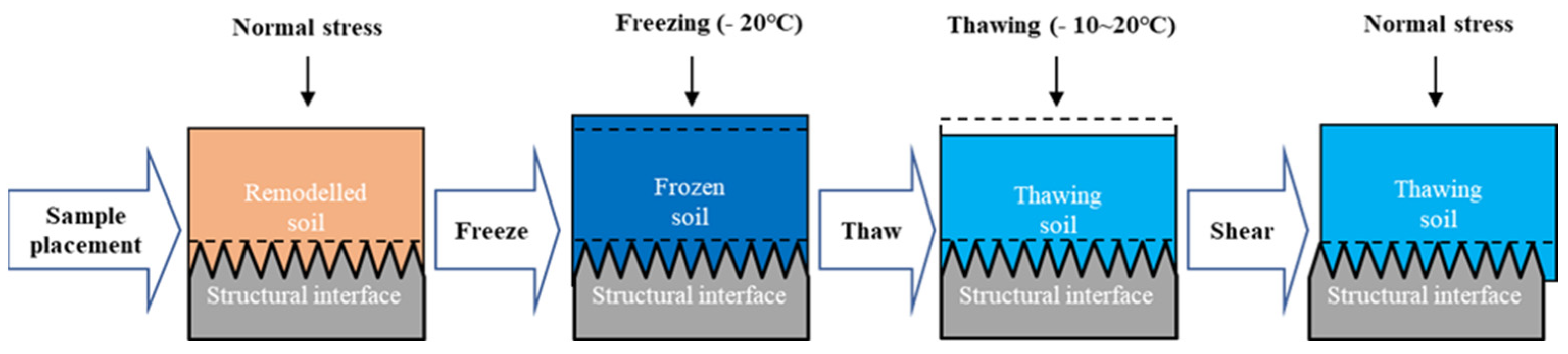
The study of the mechanical properties of the soil–structure interface is crucial for understanding the interaction between soil and underground engineering structures, making it a hot topic in geotechnical engineering [1,2,3]. In recent years, the artificial freezing method has been widely used in underground engineering construction, such as coal mine shafts, subway connecting passages, and tunnel shield originating or receiving. Consequently, the physical and mechanical properties of the frozen–thawed soil–structure interface have attracted increasing attention from researchers [4,5,6,7]. Understanding the shear behavior of the frozen–thawed soil and structure is of great significance in artificial freezing engineering design and construction.

Several researchers have explored and identified significant differences in mechanical behavior between frozen soil and other soil types. In the realm of laboratory testing, Wen et al. studied the shear stress–strain relationship and strength characteristics of the Qinghai–Tibet silt–concrete interface through direct shear tests under varying moisture content and temperature conditions [8]. Zhao et al. developed a multifunctional cyclic direct shear system for the frozen soil–structure interface and conducted shear tests under different boundary conditions [9]. Theoretical models have also been advanced. Zhou et al. established a Duncan–Chang constitutive model describing the stress–strain properties of frozen loess [10]. Liu proposed a new twin-shear strength criterion, elucidating the relationship among single-shear, twin-shear, and triple-shear strength criteria [11]. These achievements have significantly advanced the understanding of the frozen soil–structural interface. However, it should be noted that in deep underground construction using the artificial freezing method, stress in the soil increases with depth, and frost heave force is also significant under freezing conditions. Under such high stress conditions, the mechanical properties of the frozen soil–structure interface will differ significantly from those formed under conventional stress conditions.

Recently, with the development of big data mining technology and machine learning (ML) algorithms, researchers have introduced these techniques into the study of frozen soil. For instance, evolutionary polynomial regression has been used to establish the constitutive function of frozen soil [12], and artificial neural networks (ANNs) have been employed to assess soil thermal conduction [13] and to estimate various soil samples under freeze–thaw conditions [14]. The mechanical behavior of the frozen soil–structure interface is complex and difficult to describe using ordinary mathematical models [15]. Intelligent ML algorithms provide a reasonable, fast, and rigorous solution to this issue. Moreover, establishing ML models based on existing historical data is more economical than conducting laboratory measurements each time to study the mechanical behavior of the frozen soil–structure interface [2,16]. The modeling of frozen–thawed soil–structure interface shear behaviors using machine learning based on extensive indoor shear test data is limited, which deserves further exploration. In this paper, test data obtained from high normal stress and freeze–thaw direct shear tests were used to train and validate an integrated CART-based ML model. The CART algorithm is particularly suitable for small datasets and has high tolerance for data distribution. It demonstrates that the CART-based ML model has a better ability to describe the shear stress–strain relationship and strain softening phenomenon of the frozen–thawed soil–structure interface.

This paper is organized as follows: Section 2 introduces the high-stress frozen–thawed soil–structure shear test. Section 3 details the CART algorithm used in the study. Section 4 describes the process of establishing the CART-based ML model. Section 5 presents the model’s predictive performance on the stress–strain curves and analyzes the importance of various input parameters. Finally, Section 6 discusses the results.

2. Soil–Structure Interface Shear Tests

2.1. Test Instrument

The test device for examining the shear characteristics of the frozen–thawed soil–structure interface utilizes the improved direct shear test system (DRS-1), developed by the State Key Laboratory of Intelligent Construction and Healthy Operation and Maintenance of Deep Underground Engineering at the China University of Mining and Technology [17], as shown in Figure 1.

The DRS-1 system comprises four main components: a soil–structure shear box, a control system, a cooling bath device, and an acquisition system. Shear box, the primary component of the DRS-1 system, conducts direct shear tests on the soil–structure interface and can apply normal stress up to 30 MPa with a control accuracy of 1%. To maintain the specimen’s temperature conditions, the coolant in the cooling bath system must resist viscosity changes due to temperature reduction. Based on studies and laboratory measurements, ethanol glycol was selected as the circulating cooling fluid to cool the shear box through a sealed rubber tube. Additionally, the shear box is placed on a rubber plate of appropriate thickness (10 mm) to minimize heat transfer and reduce the likelihood of ambient temperature changes affecting the test results. The acquisition system collects data every 0.3 mm and automatically saves the file in .txt format. More detailed technical parameters of the DRS-1 are provided in

Table 1. DRS-1 technical parameters.

Index	DRS-1
specimen size	61.8 mm diameter
shearing mode	shear stress/strain control
normal stress range	0~30 MPa
temperature range	−40~30 °C
shear rate	0~4 mm/min
shear displacement	0~20 mm
acquisition rate	0.3 mm

.

2.2. Soil Sample and Test Process

The test soil sample is silty clay and was taken from a subway construction site in Xuzhou, Jiangsu Province, China. Its basic physical properties are listed in

Table 2. Physical properties of silty clay.

Parameters	IP (%)	D50 (mm)	Cu	Cc	wopt (%)
Value	11.0	0.06	5.83	1.38	15.1

. Based on the construction site condition, the soil specimen was prepared with a moisture content of 20% and a dry density of 1.70 g/cm³, using which the soil sample is well formed, and hardly any moisture is squeezed out during compression. The sample height of this study is 30 mm to overcome the increase in normal compression caused by the high pressure.

The structure interface is made of a uniform triangular rough steel plate, ensuring that repeated shearing does not cause wear, thereby maintaining test consistency, as shown in Figure 2.

After preparing all experimental materials, reset and adjust the control and acquisition system for each test, load the structural plate and the specimen into the shear box sequentially. The soil–structure interface shear test process involves four steps, as follows:

• Consolidation Stage: Apply the normal stress to the specimen.
• Freezing Stage: Set the corresponding freezing temperature (−20 °C for the sample).
• Thawing Stage: Adjust the circulating cold bath temperature to the target thawing temperature, start the thawing process until the sample reaches the target temperature, and maintain dynamic stability.
• Shearing Stage: During this stage, shear stress and displacement, normal load and displacement, and temperature are automatically collected and saved.

The mechanical properties of the frozen–thawed soil–structure interface are affected by many factors, such as normal stress (${\sigma }_n$), thawing temperature (T_t), roughness of structural interface (R_si), and shear rate (v), which are considered in this study. The detailed test arrangement is shown in

Table 3. Test arrangement.

Parameter	Meaning of Parameter	Parameter Range
${\sigma }_n$ (MPa)	normal stress	3, 5, 8, 10
Tt (°C)	thawing temperature	−10, −5, −2, 20
Rsi (mm)	roughness of structural surface	0, 0.9, 1.5, 3
v (mm/min)	shear rate	0.8

.

2.3. Test Result

The entire test process spanned over 180 days, during which nearly 50 groups of experiments were completed. Typical shear test results are shown in Figure 3. These results demonstrate that the shape of the shear stress–strain relationship curve is significantly influenced by the vertical pressure and thawing temperature. As vertical pressure increases, the shear stress gradually rises. Additionally, as the thawing temperature increases, the shear stress–strain curve transitions from a strain-hardening behavior (Figure 3a) to a strain-softening behavior (Figure 3b), exhibiting a distinct peak in shear stress. Further shear test results can be found in the literature [18].

3. The CART-Based Methods

The CART-based integrated algorithms, random forest (CART-RF) and adaptive boosting (CART-AdaBoost), are used to train a prediction model for the shear behavior of frozen–thawed soil–structure interface. Next, we introduce the CART and explain its integration algorithms.

3.1. CART-Based Integrated Algorithms

3.1.1. CART Algorithm

The decision tree is a tree structure in which each internal node represents a test on an attribute, each branch represents a test output, and each leaf node represents a category [19]. The most famous CART algorithm assumes that the decision tree is a binary tree and uses discretization methods to discretize continuous variables so that the model can be used for both classification and regression problems. For regression problems, the regression tree selects the minimum square error criterion as the index for evaluating split attributes. Suppose training data $D=\left\{\left(x_1,y_1\right),\left(x_2,y_2\right),...,\left(x_n,y_n\right)\right\}$, where x is the input instance, y is the output variable, then divide the input into M regions (R₁, R₂, R_m), the output value of each area is c₁, c₂, …, c_m. It is important to find the optimal regression tree model.

$$f\left(x\right)=\sum _{m=1}^M{c}_{m}I\left(x\in R_m\right)$$

(1)

The squared error is as follows:

$$\sum _{x_i\in R_m}{\left(y-f\left(x_i\right)\right)}^2$$

(2)

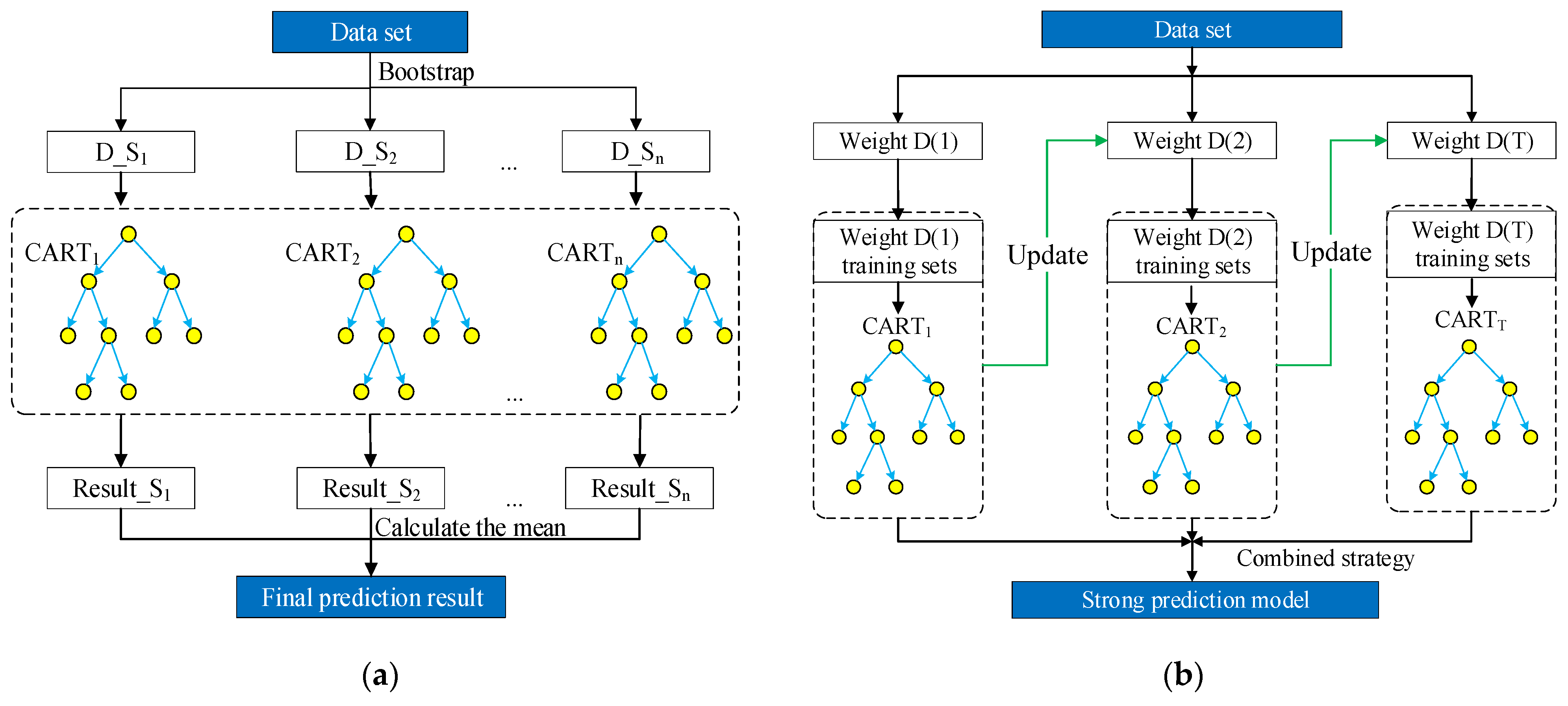
Find the optimal cut-off point for each area to minimize the model’s square error. A single decision tree selects feature variables only once at each node, lacking an iterative feedback process. This can lead to overfitting and low generalization ability on the test set. Additionally, a decision tree’s structure changes drastically with changes in the sample. To address these inherent flaws of a single model, the current popular approach involves using bagging or boosting methods to create an ensemble learning model. Among the most representative algorithms are the random forest (RF) and AdaBoost algorithms. The schematic diagram is shown in Figure 4.

3.1.2. CART-RF Algorithm

As a representative of the bagging algorithm, the CART-RF algorithm is a meta-estimator. Numerous theoretical and case studies have demonstrated that the CART-RF algorithm offers high prediction accuracy and robust tolerance for abnormal data. Using bootstrap resampling technology, multiple classification decision tree models are built on various sub-samples of the dataset. The average of these models is then used to improve predictive accuracy and control overfitting. As shown in Figure 4a, bootstrap resampling extracts n subsets from the original dataset, which serve as the training data for n CART models. The final prediction is obtained by averaging the predictions of the n CART models. The output of the CART-RF algorithm can be expressed as follows:

$$\mathrm{y}={\displaystyle \frac{1}{n}}\sum _{i=1}^n{y}_i\left(x\right)$$

(3)

where $y_i\left(x\right)$ is the individual prediction of a tree for an input x, and n is the total number of decision trees. By taking the average of the decision trees’ predictions, some errors can be canceled out. The CART-RF algorithm achieves a reduced variance by combining diverse trees, sometimes at the cost of slightly increasing bias [20]. Therefore, it is still necessary to combine domain knowledge and select reasonable model parameters to lay a good foundation for subsequent model training.

3.1.3. CART-AdaBoost Algorithm

In contrast to the bagging algorithm, the boosting method dynamically adjusts the distribution of the original training dataset, allowing base regression models to focus on challenging instances [21,22]. AdaBoost’s core concept involves training various classifiers (weak classifiers) on the same training set and subsequently combining them to create a more robust final classifier [23]. Currently, the most prevalent approach is the AdaBoost integrated algorithm, which employs CARTs as base learners. As depicted in Figure 4b, unlike the CART-RF algorithm, which selects certain variables as split variables, the CART-AdaBoost algorithm increases the likelihood of selecting samples prone to misclassification during variable selection. It then assigns weights to the output of each CART to produce the final model prediction [24]. By adjusting the distribution of sample weights, the accuracy of weak learners is enhanced.

3.2. Model Analysis Framework

Generally, two strategies can be employed to train the CART integration algorithm for modeling the behavior of frozen–thawed soil structure interfaces. One strategy involves an incremental shear stress–strain approach, gradually utilizing input and output data, while the other maintains a direct correspondence between input and output in shear stress–strain behavior [12,25]. In this study, the latter strategy is adopted for a more intuitive establishment of the relationship between input and output parameters.

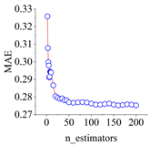
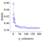
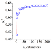
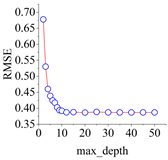
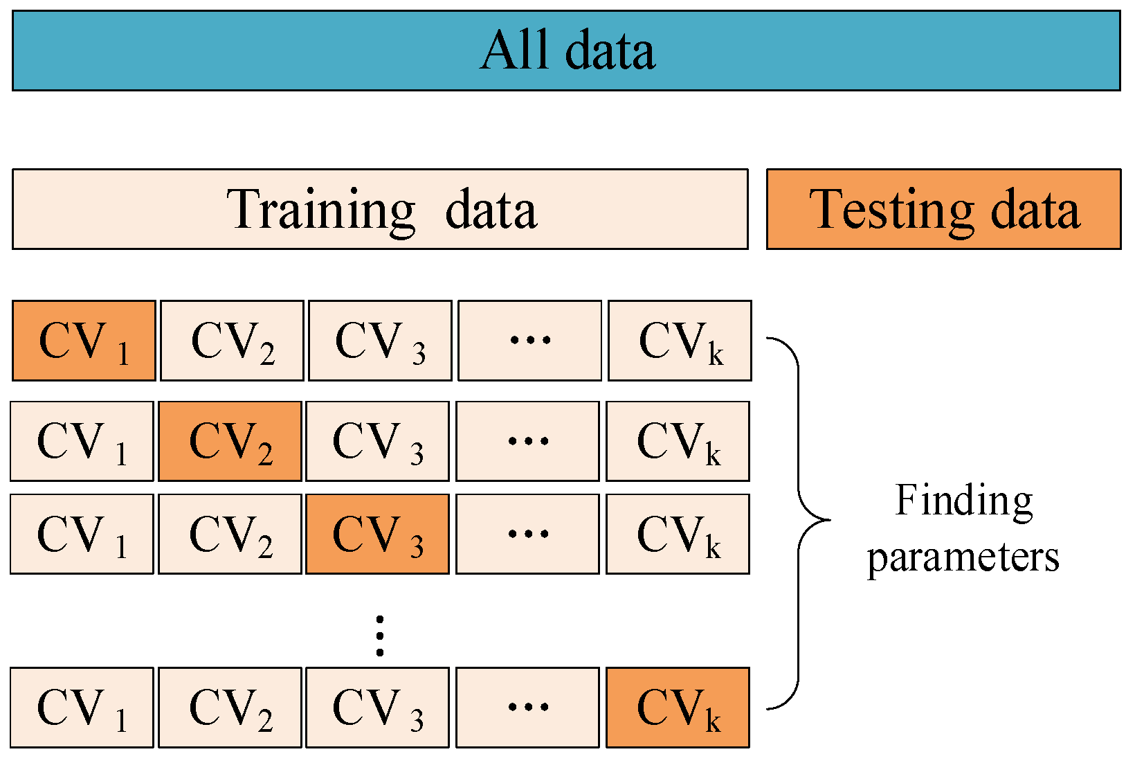
The complete model training and evaluation process for the shear stress–strain of frozen–thawed soil–structure interfaces begins with the results of the direct shear test. A data package is established, and input and output parameters are determined based on these results. The dataset is then divided into training and test sets. Subsequently, cross-validation is employed to determine the optimal hyperparameters of the model. Finally, the CART integrated prediction model, capable of describing the shear stress–strain behavior, is generated.

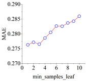
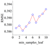
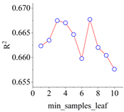
3.3. Model Evaluation Index

To evaluate the performance of the CART integrated model, this study uses three different indicators, namely, mean absolute error (MAE), average root mean square error (RMSE), and coefficient of determination (R²). MAE, RMSE, and R² are defined as follows:

$$MAE={\displaystyle \frac{1}{n}}\sum _{i=1}^n\left|f\left(x_i\right)-y_i\right|$$

(4)

$$RMSE=\sqrt{{\displaystyle \frac{1}{n}}\sum _{i=1}^n{(f\left(x_i\right)-y_i)}^2}$$

(5)

$$R^2=1-{\displaystyle \frac{\sum _{i=1}^n{(y_i-f\left(x_i\right))}^2}{\sum _{i=1}^n{(\overline{y}-\overline{f}\left(x_i\right))}^2}}$$

(6)

where $y_i$ is the true value of the sample; $f\left(x_i\right)$ is the predicted value of the model; n is the number of prediction samples; $\overline{y}$ is the average of the true values of the sample; $\overline{f}\left(x_i\right)$ is the average of the predicted values.

As indicators of regression accuracy, the RMSE and MAE are indicator types that represent the difference between model output and actual value. If the values of these indicators are particularly small, it means that the predicted output matches the recorded output well. The R² represents the proportion of variance that has been explained by the independent variables in the model. When the R² value is larger, it means that there is a strong correlation between the model output and the actual value. In the actual model, we expect lower RMSE and MAE and higher R².

3.4. Variable Importance Measures

To evaluate the importance of each input variable, this study compares the variable importance measures (VIM) of the Gini index calculated by the decision trees. The calculation method of VIM is obtained using the following equations:

$${VIM}_{jz}^{Gini}=Gini\left(X_j\right)-Gini\left(X_{r1}\right)-Gini\left(X_{r2}\right)$$

(7)

where ${VIM}_{jz}^{Gini}$ is the VIM of the $X_j$th in the node z; $Gini\left(X_{r1}\right)$ and $Gini\left(X_{r2}\right)$ are the Gini indices of the two new nodes after splitting. The VIM of $X_j$ in the ith tree is as follows:

$${VIM}_{ij}^{Gini}=\sum _{z\in M}{VIM}_{jz}^{Gini}$$

(8)

The VIM of $X_j$ in the integrated model is as follows:

$${VIM}_j^{Gini}=\sum _{i=1}^n{VIM}_{ji}^{Gini}$$

(9)

where M is the node set of the jth parameters appearing; n is the number of decision trees in the integrated model. The higher the VIM value is, the more vital the input parameters are.

4. Model Building

4.1. Data Processing

4.1.1. Input and Output Parameters

The core of realizing the shear stress (τ) prediction is to accurately grasp the key test parameters that influence the shear stress. In this study, in addition to the four influencing factors (${\sigma }_n$, Tt, Rsi, v), the shear strain (γ) and vertical displacement (s_v), which were automatically collected using the DRS-1 system during the test, were also used as the input parameters of the model. Finally, six input and one output parameters were selected as the training features of the model.

4.1.2. Dataset Segmentation

Training a predictive function’s parameters and then testing it on the same data is conducive to a methodological error: a model that simply memorizes the labels of the samples it is trained on will achieve a perfect score, yet it will not offer meaningful predictions for unseen data. To circumvent this issue, the standard practice is to split the data into two groups for supervised machine learning experiments [26]. In this study, 50 sets of test data were generated from the DRS-1 tests, totaling nearly 6060 data points. Consequently, approximately 90% of the data forms the first group used for model training, while the remaining 10% (not utilized during training) serves as the validation set to assess the model’s predictive ability. Once the dataset is partitioned, the test set comprises five data groups, as outlined in

Table 4. Indoor test conditions of the test data.

Group	${\mathit{\sigma }}_{\mathit{n}}$ (MPa)	Tt (°C)	Rsi (mm)	v (mm/min)
testing set1	8	−5	0.9	0.8
testing set2	3	−5	3	0.8
testing set3	8	−2	0.9	0.8
testing set4	10	20	0.9	0.8
testing set5	3	−10	0.9	0.8

. The distribution of prediction parameters is illustrated in Figure 5.

4.1.3. Data Normalization

The meaning, unit, and value of each physical quantity are different. If the parameters are directly sent to the model for training, the prediction accuracy of the model will be reduced. Thus, we normalize the parameters according to the standard deviation standardization method.

$$\overline{x}={\displaystyle \frac{x-u}{\sigma }}$$

(10)

where u and $\sigma$ are the mean value and the standard deviation of a dimension of the test parameters. After the training process, the results need to be transformed into the original data.

4.2. K-Fold Cross Validation

K-fold cross-validation is a popular method to determine model hyperparameters and verify the model’s validity [27]. It divides the same training data into K parts of equal size to verify a model sequentially. A fold is considered the validation data, and the rest is for training. Figure 6 is the schematic illustration of the K-fold cross-validation. The training data and test data are repeated K times; the K-1 part of the data is used to train the model, and the K part is tested. Each dataset thus has an opportunity to train and test the model. Finally, the CART integrated model with 10-fold cross-validation was selected to obtain the average evaluation indicators of the 10 sets, so as to determine the optimal hyperparameters of the model.

4.3. Determination of Hyperparameters

Hyperparameters such as max depth, min samples split, and min samples leaf in the CART are the main parameters that affect the prediction accuracy of the model. Therefore, before determining the final shear stress–strain model of the frozen–thawed soil–structure interface, the grid search (GS) method was used to determine the hyperparameters, as shown in

Table 5. Optional hyperparameters in the GS method.

Model	Hyperparameters	Range	Optimal Value	Description
CART	max_depth	2~50	10	The maximum depth of the tree; branches exceeding the maximum depth will be reduced
	min_samples_split	2~10	4	The minimum number of samples required to split an internal node
	min_samples_leaf	1~10	4	The minimum number of samples required to be at a leaf node
CART-RF	n_estimators	2~200	60	The number of trees in the forest
	max_depth	2~50	12	Same as CART
	min_samples_split	2~10	3	Same as CART
	min_samples_leaf	1~10	3	Same as CART
CART-AdaBoost	n_estimators	2~200	30	The maximum number of estimators at which boosting is terminated
	learning rate	0.01~1	1	Weight reduction factor for each weak learner
	loss function	linear, square, exponential	Linear	The loss function to use when updating the weights after each boosting iteration

. The hyperparameters of the CART-RF algorithm have one more n_estimators that characterizes the number of trees than CART. CART-AdaBoost algorithm adds two main parameters, the learning rate, which represents the weight reduction coefficient of each weak learner, and the loss function when updating the weight. Additional details of each hyperparameter can be found in the Python v.3.8 machine learning package Scikit-learn [28].

To determine the best parameters of the model, the grid search is used to traverse all the choices of hyperparameters. Take the comparison results of different hyperparameters of the CART-RF algorithm as an example, as shown in

Table 6. Comparison of different hyperparameters of the CART-RF algorithm.

	MAE	RMSE	R2
n_e
m_d
m_s_s
m_s_l

. Under different evaluation indicators, the overall prediction accuracy of the model increases with the increase in n_e and m_d. When the parameter n_e is greater than 60, the accuracy of the model on the test set is basically stable at about MAE = 0.27, RMSE = 0.38, R² = 0.66; therefore, n_e is set to 60. In the same way, m_d is set to 12. On the contrary, when the parameter values of m_s_s and m_s_l are small, the prediction accuracy of the model is high. When the parameter m_s_s is equal to 3, the best values of the three evaluation indices of the model appear (MAE = 0.276, RMSE = 0.39, R² = 0.67). Therefore, in the subsequent training, m_s_s is set to 3. Similarly, m_s_l is set to 3. The parameters of other algorithm models are the same as the CART-RF algorithm, and the best hyperparameters of different models are listed in Table 5.

5. Results and Discussion

The stress–strain dataset, which has not been introduced to the model-building process, is used to test the predictive performance of the model. The prediction results of different models for the test set are summarized in

Table 7. Prediction performance for different models.

Dataset	Evaluation Index	CART	CART-RF	CART-AdaBoost	ANN
Training set	R2	0.994	0.998	0.999	0.913
	RMSE	0.090	0.053	0.034	0.330
	MAE	0.051	0.025	0.024	0.198
Testing set1	R2	0.488	0.730	0.786	0.086
	RMSE	0.538	0.391	0.348	0.719
	MAE	0.440	0.304	0.286	0.663
Testing set2	R2	0.940	0.952	0.932	0.411
	RMSE	0.100	0.090	0.107	0.314
	MAE	0.080	0.072	0.092	0.270
Testing set3	R2	0.955	0.969	0.957	0.950
	RMSE	0.254	0.249	0.201	0.268
	MAE	0.201	0.182	0.208	0.200
Testing set4	R2	0.882	0.953	0.982	0.029
	RMSE	0.427	0.270	0.168	1.227
	MAE	0.231	0.173	0.109	1.118
Testing set5	R2	0.548	0.625	0.660	0.604
	RMSE	0.391	0.356	0.339	0.366
	MAE	0.320	0.285	0.279	0.251

. To more intuitively illustrate the predictive effect of the model, the stress–strain curves of the test set are plotted in Figure 7.

One can notice that the prediction effects are different between different models and the same model on different test sets. Both the ensemble algorithms, the CART-RF algorithm and the CART-AdaBoost algorithm, have good predictive performance for stress–strain curves under different test conditions, whether it is strain softening at high pressure with −5 °C (Figure 7a) or strain hardening at high pressure with 20 °C (Figure 7c). However, it can be seen that the prediction accuracy of the CART-AdaBoost algorithm is higher, and the predicted values were observed to essentially match the trends of the shear test results. The model can reflect the phenomenon of stress convergence in the later process of shearing. Although CART has better predictions under some experimental conditions (Figure 7b), the overall prediction performance of a single decision tree is poor.

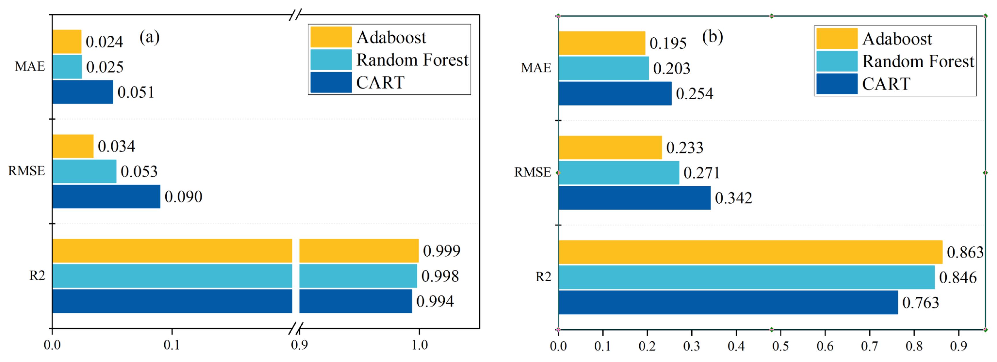
As shown in Figure 8, the accuracy of CART on the training set is R² = 0.994, while the accuracy on the test set is low (R² = 0.763), indicating that CART has poor generalization. It should be noted that, like other big data learning algorithms, the CART-RF algorithm and the CART-AdaBoost algorithm may not be able to accurately predict the material behavior outside the range of training data.

Given the size of the training dataset used in this study, we used a shallow neural network to predict the frozen–thawed soil–structure shear stress–strain curves. As we know, artificial neural network (ANN) is one of the most commonly used prediction algorithms, consisting of an input layer, hidden layers, and an output layer. According to the number of hidden layers, it is divided into a shallow or a deep neural network (DNN). Table 6 shows the performance comparison of the ANN model and the CART-based model in the dataset. For the shear stress–strain curve, the prediction effect of ANN is generally lower than that of the CART-based model, and the accuracy of ANN on the training set is much higher than the test set. Therefore, for a small dataset, we believe that the integrated CART algorithm has more advantages. Faced with big data, the ANN model may be a good choice.

As mentioned before, the VIM of the input variables is presented in

Table 8. The VIM of input variables.

Model	Normal Stress	Thawing Temperature	Roughness	Shear Rate	Strain	Vertical Stress
CART-RF	0.5751	0.0674	0.0005	0.0000	0.1706	0.1864
CART-AdaBoost	0.5994	0.0846	0.0004	0.0000	0.2316	0.0840
CART	0.5764	0.0678	0.0004	0.0000	0.1694	0.1860

. Under the test conditions, normal pressure scores the highest, followed by thawing temperature and the structural interface, while the influence of shear rate is nearly zero across different models. This indicates that the primary factors influencing the stress–strain curve are normal pressure and thawing temperature, followed by the structural interface. The VIM of input variables such as strains and vertical displacement is also high, demonstrating a strong correlation with the output.

6. Conclusions

The indoor testing method to characterize the shear behavior of frozen–thawed soil–structure interfaces often demands specialized equipment and controlled environments, making it costly, time-consuming, and sometimes unavailable. Hence, leveraging the direct shear test, we developed a CART-based integrated learning model. Through cross-validation, optimal hyperparameters of the CART-based model were determined, and subsequent comparison of the model’s prediction performance was discussed. The key findings of this study can be summarized as follows:

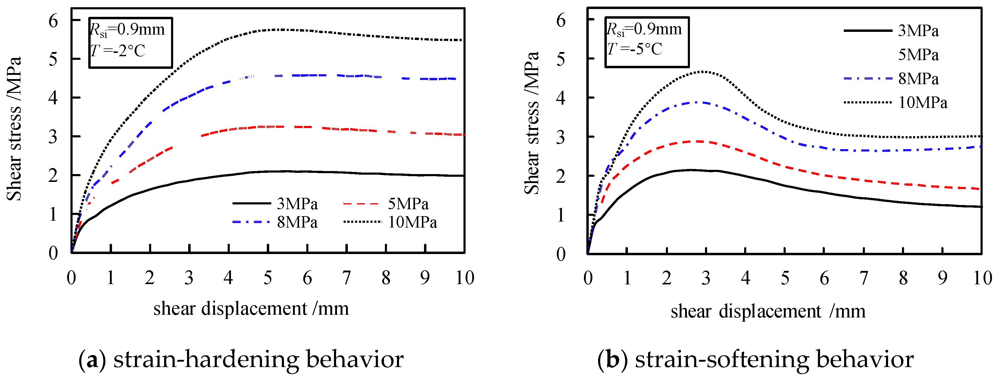
• With the increasing thawing degree of frozen soil, the shear stress–strain curves of the frozen–thawed soil–structure interfaces evolve from exhibiting characteristics of strain softening with distinct shear stress peaks to demonstrating ideal plasticity and strain hardening traits.
• While the prediction accuracy of a single decision tree proved ineffective, the integrated algorithm models (CART-RF and CART-AdaBoost) adeptly simulated the nonlinear shear behavior of a high-stress frozen–thawed soil–structure interface, successfully predicting entire shear stress–strain curves.
• Importance ranking of the influence parameters revealed that normal pressure and thawing temperature emerged as significant influencing factors for the shear behaviors of frozen–thawed soil–structure interfaces under high stress conditions.

This study represents an initial endeavor to utilize data obtained from direct shear tests. A scientifically grounded interpretation of shear stress–strain relationships, particularly employing modern machine learning technology, offers valuable insights for practitioners lacking access to testing facilities to directly simulate the mechanical behavior of thawing soil–structure interfaces. Furthermore, the pursuit of more accurate results necessitates additional experimental data, which will be addressed in subsequent research endeavors.

References

1. Hu, L.; Pu, J. Testing and modeling of soil-structure interface. J. Geotech. Geoenviron. Eng. 2004, 130, 851–860. [Google Scholar] [CrossRef]
2. Chen, W.; Luo, Q.; Liu, J.; Wang, T.; Wang, L. Modeling of frozen soil-structure interface shear behavior by supervised deep learning. Cold Reg. Sci. Technol. 2022, 200, 103589. [Google Scholar] [CrossRef]
3. Wang, H.L.; Jin, Y.F.; Yin, Z.Y.; Gu, X.Q. Uncertainty quantification of soil-structure interface properties with an enhanced hypoplastic interface model. Int. J. Geomech. 2024, 24, 04024103. [Google Scholar] [CrossRef]
4. Liu, J.K.; Lv, P.; Cui, Y.H.; Liu, J.Y. Experimental study on direct shear behavior of frozen soil-concrete interface. Cold Reg. Sci. Technol. 2014, 105, 1–6. [Google Scholar] [CrossRef]
5. Tang, L.Y.; Du, Y.; Liu, L.; Jin, L.; Yang, L.J.; Li, G.Y. Effect mechanism of unfrozen water on the frozen soil-structure interface during the freezing-thawing process. Geomech. Eng. 2020, 22, 145–254. [Google Scholar]
6. Park, S.; Hwang, C.; Choi, H.; Son, Y.; Ko, T.Y. Experimental study for application of the punch shear test to estimate adfreezing strength of frozen soil-structure interface. Geomech. Eng. 2022, 29, 281–290. [Google Scholar]
7. He, P.F.; Guo, H.; Dong, J.H.; Mu, Y.H.; Liu, F.R. Investigating the shear behavior of interfaces between frozen clay and cement blocks. J. Mater. Civ. Eng. 2024, 36, 04024076. [Google Scholar] [CrossRef]
8. Wen, Z.; Yu, Q.H.; Zhang, J.M.; Dong, S.S.; Ma, W.; Niu, F.J.; Zhao, S.P.; Yang, Z. Experimental study on adfreezing bond strength of interface between silt and foundation of Qinghai-Tibetan transmission line. Chin. J. Geotech. Eng. 2013, 35, 2262–2267. [Google Scholar]
9. Sun, H.C.; Yang, P.; Wang, G.L. Development of mechanical experimental system for interface layer between frozen soil and structure and its application. Rock Soil Mech. 2014, 35, 3636–3641. [Google Scholar]
10. Zhao, L.; Yang, P.; Zhang, L.C.; Wang, J.G. Cyclic direct shear behaviors of an artificial frozen soil-structure interface under constant normal stress and sub-zero temperature. Cold Reg. Sci. Technol. 2017, 133, 70–81. [Google Scholar] [CrossRef]
11. Zhou, Z.W.; Ma, W.; Zhang, S.; Mu, Y.; Li, G. Effect of Freeze-Thaw Cycles in Mechanical Behaviors of Frozen Loess. Cold Reg. Sci. Technol. 2018, 146, 9–18. [Google Scholar] [CrossRef]
12. Liu, X.Y.; Liu, E.L. Application of New Twin-Shear Unified Strength Criterion to Frozen Soil. Cold Reg. Sci. Technol. 2019, 167, 102857. [Google Scholar] [CrossRef]
13. Nassr, A.; Esmaeili-Falak, M.; Katebi, H. A new approach to modeling the behavior of frozen soils. Eng. Geol. 2018, 246, 82–90. [Google Scholar] [CrossRef]
14. Zhang, T.; Wang, C.J.; Liu, S.Y.; Zhang, N.; Zhang, T.W. Assessment of soil thermal conduction using artificial neural network models. Cold Reg. Sci. Technol. 2019, 169, 102907. [Google Scholar] [CrossRef]
15. Ren, J.; Vanapalli, S.K.; Han, Z.; Omenogor, K.O.; Bai, Y. The resilient moduli of five Canadian soils under wetting and freeze-thaw conditions and their estimation by using an artificial neural network model. Cold Reg. Sci. Technol. 2019, 168, 102894. [Google Scholar] [CrossRef]
16. Liu, F.Y.; Gao, C.B.; Xu, J.M.; Yang, J. Cyclic shear behavior and BoBiLSTM-based model for soil-rock mixture-concrete interfaces. Constr. Build. Mater. 2024, 426, 136031. [Google Scholar] [CrossRef]
17. Wang, B.; Xiao, H.H.; Liu, Z.Q.; Liang, Z.; Zhao, X.D. High pressure direct/residual shear test system of freeze-thawing soil structure interface and its primary application. J. Min. Saf. Eng. 2017, 34, 1194–1199. [Google Scholar]
18. Wang, B.; Liu, Z.Q.; Zhao, X.D.; Liang, Z.; Xiao, H.H. Experimental study on shearing mechanical characteristics of thawing soil and structure interface under high pressure. Rock Soil Mech. 2017, 38, 3540–3546. [Google Scholar]
19. Abellan, J.; Mantas, C.J.; Castellano, J.G. A random forest approach using imprecise probabilities. Knowl. Based Syst. 2017, 134, 72–84. [Google Scholar] [CrossRef]
20. Mbarak, W.K.; Cinicioglu, E.N.; Cinicioglu, O. SPT based determination of undrained shear strength: Regression models and machine learning. Front. Struct. Civ. Eng. 2020, 14, 185–198. [Google Scholar] [CrossRef]
21. Wang, C.; Yang, C.; Qin, H.; Wang, Y. Examination of determinants and predictive modeling of artificially frozen soil strength utilizing the XGBoost algorithm. Appl. Sci. 2023, 13, 13170. [Google Scholar] [CrossRef]
22. Xiao, H.; Xing, B.; Wang, Y.; Yu, P.; Liu, L.; Cao, R. Prediction of shield machine attitude based on various artificial intelligence technologies. Appl. Sci. 2021, 11, 10264. [Google Scholar] [CrossRef]
23. Freund, Y.; Schapire, R.E. A decision-theoretic generalization of on-line learning and an application to boosting. J. Comput. Syst. Sci. 1997, 55, 119–139. [Google Scholar] [CrossRef]
24. Liu, Q.S.; Wang, X.Y.; Huang, X.; Yin, X. Prediction model of rock mass class using classification and regression tree integrated AdaBoost algorithm based on TBM driving data. Tunn. Undergr. Space Technol. 2020, 106, 2020. [Google Scholar] [CrossRef]
25. Faramarzi, A.; Javadi, A.A.; Alani, A.M. EPR-based material modelling of soils considering volume changes. Comput. Geosci. 2012, 48, 73–85. [Google Scholar] [CrossRef]
26. Ghorbani, B.; Arulrajah, A.; Narsilio, G.; Horpibulsuk, S. Experimental and ANN analysis of temperature effects on the permanent deformation properties of demolition wastes. Trans. Geotech. 2020, 24, 100365. [Google Scholar] [CrossRef]
27. Hasanpour, R.; Rostami, J.; Jürgen, S.; Ozcelik, Y.; Sohrabian, B. Prediction of TBM jamming risk in squeezing grounds using Bayesian and artificial neural networks. J. Rock Mech. Geotech. Eng. 2020, 12, 21–31. [Google Scholar] [CrossRef]
28. Swami, A.; Jain, R. Scikit-learn: Machine Learning in Python. J. Mach. Learn. Res. 2013, 12, 2825–2830. [Google Scholar]
Figure 1. DRS-1 test system.
Applsci 15 04806 g001
Figure 2. Schematic of the shear test process.
Applsci 15 04806 g002
Figure 3. Typical results of the direct shear tests.
Applsci 15 04806 g003
Figure 4. The schematic illustration of the CART-based algorithms: (a) CART-RF algorithm; (b) CART-AdaBoost algorithm.
Applsci 15 04806 g004
Figure 5. Distribution of the predicted shear stress.
Applsci 15 04806 g005
Figure 6. The schematic illustration of the K-fold cross-validation.
Applsci 15 04806 g006
Figure 7. Comparison of prediction results under different models with experimental data: (a) testing set 2; (b) testing set 3; (c) testing set 4.
Applsci 15 04806 g007
Figure 8. Regression performance of the CART-AdaBoost algorithm, CART-RF algorithm, and CART (a) training set; (b) testing set.
Applsci 15 04806 g008