Abstract
Machine learning (ML) algorithms have been developed for cost performance prediction in the form of single-point estimates where they provide only a definitive value. This approach, however, often overlooks the vital influence project complexity exerts on estimation accuracy. This study addresses this limitation by presenting ML models that include interval predictions and integrating a complexity index that accounts for project size and duration. Utilizing a database of 122 infrastructure projects from public works departments totaling HKD 5465 billion (equivalent to USD 701 billion), this study involved training and evaluating seven ML algorithms. Artificial neural networks (ANNs) were identified as the most effective, and the complexity index integration increased the R2 for ANN-based single-point estimation from 0.808 to 0.889. In addition, methods such as bootstrapping and Monte Carlo dropout were employed for interval predictions, which resulted in significant improvements in prediction accuracy when the complexity index was incorporated. These findings not only advance the theoretical framework of ML algorithms for cost contingency prediction by implementing interval predictions but also provide practitioners with improved ML-based tools for more accurate infrastructure project cost performance predictions.
1. Introduction
Uncertainty is inherent to infrastructure projects, arising from factors such as changing site conditions, fluctuating material costs, and unforeseen technical challenges [1,2]. To manage these uncertainties, contingency funds are typically allocated [3]. Traditional methods of contingency estimation often rely on subjective judgment, such as expert interviews or surveys, or simulation techniques, such as Monte Carlo simulations [3,4,5]. However, reliance on the above subjective judgments is often criticized for its inconsistencies and potential bias [6]. Similarly, simulation-based methods depend on underlying assumptions that may not fully capture the complexity of real-world projects. Infrastructure projects, in particular, entail elevated levels of risk and unpredictability due to their large scale, complexity, and extended timelines [7,8]. These characteristics make determining an appropriate contingency allocation especially challenging. Therefore, the development of predictive methods capable of addressing the uncertainty and complexity of infrastructure projects is essential.
Conversely, ML algorithms offer a promising alternative by leveraging data to identify complex, non-linear relations among project variables [9]. ML enables practitioners to anticipate and quantify potential uncertainties more effectively. Research by El-Kholy et al. [10] demonstrated that ML models outperformed traditional estimation techniques, such as regression-based models, in terms of accuracy. ML also offers a more reliable approach to accounting for uncertainties and improves financial planning in construction projects. Several studies have explored the potential of using ML to estimate cost contingencies [1,11]. However, previous studies have predominantly utilized ANNs or linear regression models and often focused on project risk factors rather than the distinct characteristics of individual projects [5]. This highlights a research gap in evaluating diverse ML models to identify those offering superior predictive performance. Incorporating project-specific attributes, such as scale and project duration, would allow these models to better capture the inherent uncertainties that should be accommodated in contingency estimates.
In addition to technical challenges, project complexity plays a critical role in cost outcomes and affects the accuracy of cost estimation [12,13,14]. The evidence suggests that complexity level has a substantial effect on cost performance [15]. Moreover, prior research has also found that complexity affects the accuracy of cost estimation [16]. Thus, a measure of project complexity is necessary to accurately reflect a project’s multifaceted nature when applying ML algorithms to infrastructure projects. A complexity index, which integrates factors such as project scale and capital investment, offers a more comprehensive measure of project risk and the potential of unforeseen challenges during project execution [17]. However, relatively few studies have incorporated a complexity index to capture the multifaceted nature of infrastructure project environments [1]. This study attempts to integrate a complexity index to improve the accuracy and robustness of cost contingency predictions. This approach is particularly valuable in contexts of significant project complexity, such as large-scale infrastructure projects.
Moreover, human cognitive biases also affect the confidence of project cost estimation. A natural aversion to uncertainty often makes project planners reluctant to fully trust point estimates, as project outcomes are inherently unpredictable [18]. Furthermore, reliance on a single-value prediction that does not account for a range of potential outcomes can result in underestimating risks [19]. Formatting cost estimates as interval ranges rather than fixed points mitigates these issues by explicitly acknowledging uncertainty. Confidence intervals, grounded in statistical sampling principles, provide a robust framework for capturing and communicating uncertainty [20]. Despite these advantages, few studies provide confidence intervals for cost contingency estimation [5]. To equip project planners with a realistic range of potential cost outcomes in the form of contingency intervals, advanced uncertainty estimation techniques are needed.
Therefore, an important question arises: how can ML techniques enhance the forecast performance of infrastructure cost contingency materialization, especially for projects with high complexity levels?
To answer this question, this study has three main research objectives:
- (1)
- To select high-performing ML models for cost contingency prediction;
- (2)
- To investigate whether integrating a complexity index can improve prediction performance;
- (3)
- To develop interval predictions and assess whether the incorporation of a complexity index improves their accuracy.
To achieve these objectives, this study used a dataset of 122 Hong Kong infrastructure projects for model development. Seven ML algorithms were examined for cost contingency prediction. Linear regression and support vector regression (SVR) serve as baseline models, offering interpretability but limited capability in capturing non-linear relationships. Tree-based methods, including decision trees, random forest, gradient boosting, and extreme gradient boosting (XGBoost), leverage hierarchical structures to model variable interactions. Finally, ANNs employ interconnected layers of neurons to capture intricate, non-linear relationships. In addition to point predictions, this study incorporates two interval estimation methods, Monte Carlo dropout and bootstrapping, to quantify model uncertainty. Monte Carlo dropout introduces randomness in neural network predictions, while bootstrapping generates multiple resampled datasets to assess prediction variability.
This research contributes to the cost contingency literature in three key ways. First, it employs and compares seven ML algorithms by systematically assessing their predictive performance in cost contingency estimation. Second, it introduces interval prediction methods to capture model uncertainty. To the best of the authors’ knowledge, this is the first study to apply interval estimations in cost contingency prediction. Third, it develops a complexity index that accounts for project scope and duration to improve the accuracy of point and interval estimates. These contributions collectively advance the application of ML in cost contingency estimation by improving predictive accuracy and uncertainty quantification.
2. Literature Review
2.1. Cost Contingency Prediction
Contingency can be defined as the amount of funds, budget, or time needed in addition to the estimate to reduce the risk of project objective overruns to a level that is acceptable to the organization [17]. This study specifically examines cost contingency, where a portion of the project budget is set aside to cover the unforeseen risks or challenges that may occur during a project. This allocation functions as a financial buffer for unexpected expenses beyond the initial project scope, such as design changes, material cost changes, delays, or unforeseen site conditions [11,17]. Typically, cost contingency is determined as a percentage of the total project cost that is informed by historical data and adjusted for factors such as project complexity, risk assessments, and client requirements [2]. Previous research has employed both traditional estimation methods and ML approaches to estimate cost contingency.
2.2. Traditional Approaches to Contingency Estimation
Traditional contingency estimation often relies on expert judgment [5,21], questionnaire surveys [4,22], and simulation analysis [3,23,24]. Questionnaires have proven effective in identifying factors that could influence contingency estimates or cost overruns. The determinants of contingency funds, such as contract type, advance payment amount, and the availability of construction materials, are often revealed through questionnaire surveys [4,17,22]. Furthermore, expert judgment also plays a significant role in this process. For example, Idrus et al. [21] developed a fuzzy expert system for cost contingency estimation based on risk analysis and achieved reasonable accuracy. Similarly, Islam et al. [5], informed by industry experts, identified cost overrun risks and developed a probabilistic risk network to guide contingency estimation.
Conversely, Monte Carlo simulation and parametric modeling have also been applied to estimate contingency funds. Barraza et al. [23] used Monte Carlo simulation to capture the probabilistic nature of project costs. They assumed a normal distribution of project costs. The target cost was set as the mean of the project cost, while the planned budget was established at the 80th percentile. The difference between these two values was then treated as an estimated contingency. Similarly, Hammad et al. [3] applied Monte Carlo simulation to manage cost contingency during project implementation. By assessing the contingency that arose in specific activities and the proportionate cost of these activities compared to the overall project, they calculated the remaining contingency. In addition to Monte Carlo simulation, Thal Jr. et al. [24] used parametric modeling for contingency prediction and identified critical factors that affect contingency estimates, such as project characteristics, design performance metrics, and contract award processes. A regression model was then developed based on these factors.
2.3. Machine Learning Applications in Contingency Estimation
Commonly used ML algorithms in construction management studies include linear regression, support vector machine (SVM), tree-based methods (such as decision trees, random forests, gradient boosting, and XGBoost), and ANNs [9]. Table 1 presents their theoretical underpinnings and strengths.
Linear regression predicts continuous outcomes in terms of one or more input variables [25]. It aims to achieve the optimal fit between the input variables and the target by minimizing the ordinary least squares (see Table 1 for the theoretical grounding). This method is easy to understand and interpret, performs well for linear relationships, and is computationally efficient [9,26]. However, its performance can lag behind more advanced ML algorithms, particularly when capturing complex, non-linear relations [26]. SVM can find an optimal hyperplane to separate the data points in multiple dimensions [9]. SVR, a variant of SVM, extends this concept to regression by fitting a function within a defined margin around the hyperplane to predict continuous outcomes. SVR is robust to outliers and can effectively handle complex, non-linear data [27]. Linear regression and SVR are often employed as foundational models in predictive analysis due to their simplicity and interpretability [28].
Tree-based methods, including decision trees, random forests, gradient boosting, and XGBoost, are known for their versatility and ability to capture complex, non-linear relations [26]. Of these methods, decision trees are the simplest. They are powerful tools for capturing non-linear relationships and identifying feature importance without extensive data preprocessing [9]. However, individual trees can overfit the data. Random forests can address overfitting by combining multiple decision trees and averaging their outcomes [29,30]. Gradient boosting further improves prediction by sequentially building trees where each tree corrects the errors of its predecessor, producing a strong ensemble model [31]. XGBoost further develops gradient boosting by adding regularization and optimization techniques that reduce overfitting and increase efficiency [32]. Studies in construction management have found that XGBoost provides the highest predictive performance of the tree-based methods [9].
ANNs are inspired by the structure of the human brain, where neurons connect and transmit signals to process information [33]. This structure enables ANNs to identify complex patterns in data, making them highly effective for handling non-linear data, as in cost and contingency estimation [1,33], project duration prediction [28], and project risk assessment [34] in the construction industry.
In the last decade, ML algorithms have been applied to cost and contingency estimation. Although numerous ML models have been developed for cost prediction [31,32,35], few studies have focused on cost contingency estimation. Table 2 summarizes the previous studies that applied ML to the predictive analysis of cost contingency. Lhee et al. [1] were among the first to use ML for cost contingency estimation in construction projects, employing an ANN to estimate optimal contingency levels. Their approach used an intermediate contingency form—the contingency rate—as the neural network’s output variable to predict the owner’s contingency. The ANN model developed was based on only four project characteristics (the number of bidders, project letting year, project duration, and contract value), which may limit its capacity to capture the broader uncertainties affecting cost outcomes.

Table 2.
Previous studies of cost contingency prediction using machine learning.
Table 1.
ML algorithms and their theoretical underpinnings and strengths.
Table 1.
ML algorithms and their theoretical underpinnings and strengths.
| Algorithms | Theoretical Underpinnings | Strengths |
|---|---|---|
| Linear regression | Linear regression assumes a linear relationship between the input variables and the target: where is the predicted target, represents the input variables, are the coefficients (weights) that quantify the influence of each input on the target, and is the intercept. The optimal coefficients are achieved by minimizing the ordinary least squares [11]: , where is the actual value, is the predicted value, and is the number of observations. The coefficients in the linear regression model quantify the influence of each input variable on the target. | Simplicity, interpretability, and computational efficiency |
| SVR | Similar to linear regression, SVR fits the function WTX + b while allowing a margin of tolerance . To handle non-linear relations, it performs the kernel trick, which maps data to a higher-dimensional space where linear separation is achievable. Common kernel options include linear (), polynomial, and radial basis function [27]. | Capability to address outliers and model non-linear relationships |
| Decision trees | Decision trees split data into branches based on features that best reduce impurity. Impurity is a measure of the homogeneity of the data within a node, aiming to make each split as “pure” as possible. It can be calculated using metrics like Gini impurity and entropy for classification and variance for regression models [25]. Specifically, Gini impurity is calculated as: , where is the proportion of class in the node ; and entropy is measured as: . | Capability to model non-linear relationship and effectively identify important features |
| Random forest | Random forest improves predictive accuracy by combining multiple decision trees. Each tree is trained on a random subset of data and features, reducing variance and overfitting [26]. The final prediction is the average outcome across all trees: , where is the total number of trees. | Robustness to overfitting |
| Gradient boosting | Gradient boosting builds an ensemble of decision trees sequentially, with each new tree focused on reducing the errors of the previous one [36]. At each step , the model updates predictions as: , where is the learning rate controlling the contribution of each tree. The final model combines these sequentially trained trees, each contributing based on its ability to minimize prior errors. | Promising predictive accuracy through interactive error correction |
| XGBoost | XGBoost employs regularization and optimization techniques to enhance model performance. Regularization, which prevents overfitting by penalizing model complexity, includes two techniques: L1 and L2 [31]. L1 regularization applies a penalty based on the absolute magnitude of coefficients, given by , while L2 uses the squared magnitude, i.e., , where are model parameters, and and control the strength of L1 and L2 regularization, respectively. XGBoost also uses optimization techniques, like second-order approximation and shrinkage. | High predictive accuracy through optimization |
| ANN | An ANN consists of interconnected neuron layers: input, hidden, and output. Each neuron in layer l receives weighted inputs from the previous layer : , where and refer to the weight and bias, respectively. The activation function introduces non-linearity: . During training, the ANN adjusts these weights using backpropagation which calculates the gradient of the loss function (a measure of prediction error) with respect to each weight [28]. | Ability to model complex relationships |
More recently, Islam et al. [5] employed Bayesian belief networks to estimate the probability of cost overruns, focusing on cost overrun-related risks. While a promising estimate can be provided by their Bayesian model, the extensive subjective input and requirement for prior probability data may constrain the model’s applicability. El-Kholy et al. [10] compared ANNs with regression-based models for contingency estimation, focusing on contractors’ approaches to managing cost-related risks. Their results indicate that ANNs provide superior predictive performance. However, the study primarily focused on the influence of steel reinforcement prices, reflecting only a narrow subset of the factors affecting cost contingency. Furthermore, the datasets used by Islam et al. [5] and El-Kholy et al. [10] were limited, with only 12 and 30 projects, respectively. Similarly, Ammar et al. [11] developed a linear regression model to estimate contingency based on cost overrun risks, but this model also lacks diverse project features as input variables and depends heavily on subjective input data.
In summary, despite the increasing interest in ML for cost contingency estimation, the existing studies are limited by their reliance on narrow project-specific characteristics, subjective risk inputs, and a restricted selection of ML algorithms, primarily ANNs and linear regression models [1,10,11]. Expanding the use of ML algorithms to include diverse project-specific characteristics and testing a broader range of algorithms could significantly advance the contingency estimation literature.
2.4. Interval Estimation in Machine Learning
Interval estimation in ML provides a range in which a predicted value is expected to fall, offering a more comprehensive understanding than point predictions alone [37]. While point estimates give a single predicted value, they fail to account for model uncertainty. In contrast, interval estimates reflect prediction uncertainty with a confidence level [20]. This can be crucial in high-stakes applications, such as medical diagnosis [38], unsafe event prediction [39], and construction cost estimation [9]. Common techniques for interval estimation include quantile regression, Bayesian neural networks, Monte Carlo dropout, and bagging [38,39,40]. These approaches account for either uncertainty in the model parameters or input data variability for interval estimates. By conveying the confidence level associated with predictions, interval estimates can support more robust decision-making by providing probabilistic boundaries for their outputs [18,19]. As a result, interval estimates are especially useful in projects that require risk assessment, safety margin considerations, and contingency planning, enabling project managers to anticipate variance and adopt proactive measures to address uncertainty.
Several studies have applied interval estimation to construction management, particularly for classification prediction [40,41]. These studies primarily employed Bayesian ML approaches. Gondia et al. [41] utilized decision trees and naïve Bayesian classification algorithms to predict the project delay risk, categorizing the output into three classes: less than 30%, between 30% and 60%, and more than 60% schedule overrun. More recently, Wu et al. [39] combined a Bayesian framework with ML algorithms to create a binary Bayesian inference model, while Vassilev et al. [42] extended neural networks to develop a Bayesian deep-learning model. However, none of these studies have applied interval estimation specifically to cost or contingency estimation. Furthermore, as the Bayesian approach relies on prior probability data and involves computational complexity, it can be challenging to apply in scenarios that lack prior probability data [5]. To address these data and computational challenges, methods approximating Bayesian techniques can be employed instead [19].
2.5. Project Complexity and Estimation Accuracy
Project complexity is defined as the property of a project that makes it difficult to understand, foresee, and control its overall behavior, even when reasonably complete information about the project system is available [43]. High-complexity projects often have unclear functional requirements and ambiguous objectives, with work content that requires further development during the project [7,44]. These inherent uncertainties in complex projects increase the difficulty of accurately predicting cost outcomes.
The evidence shows that project complexity often affects estimation accuracy. Hatamleh et al. [45] identified project complexity as the most pronounced project characteristic that affects the accuracy of cost estimates. High project complexity—characterized by extended planning horizons, larger budgets, increased technical demands, higher expectations of innovation, and interconnected interfaces—introduces greater uncertainty [15,46]. As complexity grows, the number of unpredictable variables rises, increasing the likelihood of deviations from initial estimates [47]. In addition, high-complexity projects are often large-scale with long durations, allowing even minor deviations to escalate into major shifts as multiple factors interact and amplify their effects. Optimism bias exacerbates performance evaluation challenges as project planners tend to understate potential risks and overestimate project outcomes, particularly in complex projects [48]. Thus, achieving high estimation accuracy in complex projects remains a significant challenge that requires advanced techniques to account for the multifaceted nature of these projects.
Empirical studies highlight the significant influence of project complexity on cost outcomes. Flyvbjerg [13] found that complex projects often encounter substantial cost overruns due to unpredictable factors, and only one in ten large-scale infrastructure projects are delivered on time. Similarly, Doyle and Hughes [16] demonstrated a strong correlation between project complexity and the reliability of cost estimation. In addition, Asmussen et al. [49] revealed that structural complexity particularly reduces cost estimation accuracy in supply chain design as it introduces more conflicting goals. These findings underscore the importance of incorporating complexity measures to better capture the high uncertainty associated with high complexity.
2.6. Research Gap
In summary, while the existing studies provide valuable insights, notable research gaps persist in terms of cost contingency estimation. First, most studies employ a limited selection of ML algorithms, mainly ANNs and linear regression. This may restrict the potential for increasing the accuracy and robustness of predictions. Furthermore, few ML models for contingency estimation incorporate project-specific characteristics, which are essential for capturing unique project dynamics and improving estimation precision. Another key limitation is the absence of interval estimation techniques in contingency models, although these would define a range of probable values and offer project managers a clearer understanding of potential cost variability. Finally, project complexity, although it is a critical factor affecting estimation accuracy, is rarely integrated into current models. This may limit the ability to account for the nuances affecting cost performance, especially for relatively complex infrastructure projects. Therefore, addressing these gaps could significantly advance contingency estimation methods and produce more reliable and adaptable tools for infrastructure project cost management.
3. Materials and Methods
This study comprised four main stages: data collection and preprocessing, project contingency prediction models, ANN and complexity index creation, and interval predictions and complexity index use (see Figure 1).

Figure 1.
Research design.
3.1. Stage 1: Data Collection and Preprocessing
In this stage, data were collected and preprocessed, which included data cleaning, feature selection, and feature scaling. A total of 122 infrastructure project cases were collected from the Hong Kong Public Works Department. Projects were included based on their classification as infrastructure, which was determined according to official categorization by the department. Specifically, the dataset encompassed projects related to transportation (e.g., roads, bridges, and tunnels), utilities (e.g., water supply and drainage systems), and public facilities (e.g., government buildings and hospitals). Only completed projects with available records on cost estimates, contingency allocations, and actual expenditures were considered to ensure data reliability and comparability. During the data collection process, relevant project data, including project characteristics, project estimates (PEs), contract contingencies, and approved PEs under public budget allocation, were gathered.
Data cleaning was performed to remove duplicates and address missing data. The dataset was constructed by integrating various types of projects, including land development projects (LDPs), roads and highways (RH), water treatment projects (WTPs), sewage treatment projects (STPs), and other public functional projects (PFPs, e.g., hospitals, schools, and government offices). Given the integration of diverse project types, potential duplicates were identified and removed using the drop_duplicates() function in Pandas to ensure unique entries across the dataset. Missing data were handled through either imputation or removal, depending on the extent of the missing values, to maintain dataset reliability and facilitate accurate predictions [36,50]. Features with more than 30% missing data were excluded, while those with less than 30% missing data were retained, and the missing values were imputed [51]. For this study, two imputation approaches were considered: (i) replacing missing values with the mean or median or (ii) estimating the missing values more precisely based on underlying data patterns [52]. Although the first method is straightforward, it can reduce data variability and introduce bias. Therefore, the second approach was adopted, and a linear regression model was used for imputation. This method preserved the data patterns and improved the consistency of the predictive models.
A set of seven input variables, including PE, contract contingency, approved PE, project type, starting and completion years, and project scope, was created and used for model development. These variables were selected because they represent key factors influencing the cost and contingency outcomes in infrastructure projects. Specifically, the PE and approved PE capture the project’s initial cost assessments [45]; contract contingency reflects the risk management buffer embedded into the project budget [2]; and project type accounts for variations in project characteristics. The starting and completion years were included to reflect temporal aspects, such as inflation and regulatory changes [28,32]. The construction floor area variable indicated project size. This set of input variables was deemed appropriate as it encompasses both financial planning and inherent project characteristics, which are vital for modeling cost performance and contingency materialization and, therefore, provide a robust foundation for prediction models. After data cleaning, the “project scope” variable was excluded due to a missing data rate of more than 30%. The six remaining features were retained for model development.
The target variable value, cost contingency, was calculated in terms of final cost, project estimate, and contract contingency due to the absence of direct data records for cost contingency values. The materialized cost contingency is defined as the difference between the final cost and the project cost [3]. The project cost is equivalent to the approved project estimate minus the contract contingency. Therefore, the cost contingency was derived using the following formula:
Cost contingency = Final cost − (Approved project estimate − Contract contingency)
In feature scaling, the input variables are transformed into a standardized range, commonly between 0 and 1 [35]. This transformation is essential to improve model performance and stability, particularly when the dataset features high standard deviations [28]. The scaling procedure was implemented using Equation (2), as shown below:
where is the transformed value of the original value , and and refer to the minimum and maximum values of the set of attribute .
To mitigate potential overfitting and determine the optimal ML model, the dataset of 122 project cases was randomly divided into two subsets, and 80% of the data was allocated to the training set, while the remaining 20% was used as the testing set [32,53]. The model’s performance based on the testing set is presented as the final result.
3.2. Stage 2: Project Contingency Prediction Models
This stage focused on developing and evaluating ML models for cost contingency prediction. Seven models were considered: linear regression, SVM, decision trees, random forests, gradient boost, XGBoost, and ANNs. These models were selected for (i) their widespread use in cost and contingency prediction and (ii) their broad capacity to handle different predictive tasks (see Table 2) [9]. Linear regression functioned as a baseline model due to its straightforward approach to cost prediction. SVM was chosen for its ability to capture complex relationships between input features and cost outcomes [28,36]. Decision trees, which model non-linear relationships, were supported by random forests through ensemble learning to improve prediction accuracy [30]. Gradient boosting and XGBoost were included for their focus on iterative error correction and performance optimization [32]. ANNs were utilized for their strength in capturing intricate, non-linear interactions between features [33,35]. Together, these models facilitated a robust comparison analysis to identify the best-performing algorithm for contingency prediction.
Each model was systematically fine-tuned to enhance its predictive accuracy and reliability. A grid search was employed to identify the optimal hyperparameters by systematically exploring predefined parameter ranges and evaluating all possible combinations [54]. Cross-validation was then used to assess model performance and prevent overfitting [55]. The final selection of hyperparameters was based on minimizing prediction error metrics. The optimal hyperparameters derived through this process are presented in Table 3. This tuning approach allowed for systematically evaluating various parameter combinations and enabled the selection of the most appropriate settings for each algorithm [56].
Table 3.
Fine-tuned hyperparameters for the model algorithms.
Then, the performance of each model was evaluated and compared through key metrics, including R2, mean absolute error (MAE), mean square error (MSE), and root mean square error (RMSE) [28]. These metrics were employed to assess the models’ accuracy and robustness in predicting outcomes. R2 measures the proportion of variance in the dependent variable that can be explained by the independent variables. It ranges in value from 0 to 1, with values closer to 1 indicating a better model fit [9]. The calculation of R2 is expressed by Equation (3).
where is the actual value, is the predicted value, is the mean of actual values, and is the number of project cases.
MAE measures the average of the absolute errors between predicted and actual values [36]. It is a straightforward measure of prediction accuracy calculated as shown in Equation (4):
RMSE is the square root of MSE, which offers a metric by squaring the residuals (the differences between the predicted and actual values). Compared to MAE, it weights larger errors more, which can be useful when larger errors are more impactful. Equations (5) and (6) were used to calculate MSE and RMSE, respectively:
According to the evaluation of model performance metrics, the high-performing models were then selected for further analysis due to their superior predictive capabilities and reliability.
3.3. Stage 3: Point Estimation and Complexity Index
In this stage, the top-performing models from Stage 2 were used to generate point estimates for materialized cost contingency. To assess the influence of the complexity index, two versions of each model were developed: one excluding the complexity index and one incorporating it. A feature importance analysis was conducted to quantify the contribution of each input variable, particularly the complexity index, in enhancing predictive accuracy. The methodology for measuring the complexity index and computing feature importance is detailed in the following sections.
Project scope is a crucial determinant of project complexity [15]. Unlike other complexity indices, such as expert interviews to measure technological and environmental complexity [57], which rely heavily on subjective data, scope complexity can be qualified with objective project data. This makes it a readily measurable metric for categorizing construction projects. Therefore, scope complexity was selected to quantify the complexity index used in this study. Nguyen et al. [58] identified project size (in terms of capital), scope ambiguity, and project duration as key determinants of scope complexity. Due to data availability, this study focuses on two measurable factors for the complexity index: project size (capital) and project duration. Each factor is weighted equally (50:50) in the index calculation. The construction of the complexity index is outlined as follows:
To classify project complexity by size and duration, a quantile-based approach was applied. This approach facilitated a straightforward division of projects based on their relative capital size and duration, ensuring objectivity grounded in the dataset distribution. Projects were divided into five categories according to their position within predefined quantile ranges, ensuring objective categories according to the distribution of the dataset. Specifically, a scale of 1 to 5 was used, where projects falling within the [0.8, 1.0] quartile range were assigned a complexity score of 5, those within the [0.6, 0.8] range were assigned a score of 4, etc. Projects within the lowest quartile were assigned a score of 1. The final complexity index is calculated as the average of the two scores, providing an objective and scalable measure of project complexity. This approach standardized the complexity index, enabling consistent comparisons across diverse project cases.
Second, feature importance quantifies the contribution each input feature makes to the predictions made by an ML model [28]. It identifies the most significant features for accurate predictions by evaluating their impact on the model outcome. Depending on the algorithm, various techniques can be used to determine feature importance. As the ANN was the contingency estimation model with the most promising predictive performance in Stage 2, permutation feature importance was conducted at this stage [59]. This works by randomly shuffling the values of a single feature and then measuring the change in the model’s performance [60]. If the performance drops significantly when a feature is permuted, that feature is considered important because it has a critical effect on the prediction model. Conversely, if shuffling a feature results in little to no performance change, the feature is considered less important. The permutation importance of a feature is computed as follows:
where is the permutation importance of feature , and and are the model performance before and after shuffling, respectively. The baseline and permuted performance can be assessed with any of the metrics discussed in Stage 2, including R2, MAE, MSE, and RMSE. In this study, MSE was used to evaluate changes in performance.
3.4. Stage 4: Interval Predictions and Complexity Index
Stage 4 involved generating interval predictions using two methods: Monte Carlo dropout and bootstrapping (see Figure 1). These techniques leverage resampling or dropout as Bayesian approximations, enabling the model to quantify uncertainty and generate prediction intervals based on the output variance [38,61]. Compared to traditional Bayesian methods, these two techniques allow the quantification of uncertainty in datasets that lack explicitly probabilistic information [19,42]. Therefore, they were adopted in this study to increase the robustness of the prediction models. As in Stage 3, two interval prediction models—one excluding the complexity index and one incorporating it—were compared to evaluate the impact of the complexity index on predictive accuracy. The evaluation method for interval predictions followed Milanés-Hermosilla et al.’s [38] approach, where uncertainty accuracy was used to assess the performance of uncertainty estimations. The approaches and evaluation processes for the interval predictions are detailed below:
- (a)
- Monte Carlo dropout
Monte Carlo dropout was applied to obtain interval predictions by performing multiple stochastic forward passes through the ANN [38]. Fundamentally, the Monte Carlo dropout approach involves executing the model n times with dropout enabled to introduce randomness in the network’s weights during inference and generate different predictions for the same test case x [62]. The Monte Carlo dropout process consists of four steps:
- (i)
- Train the model using the original training dataset, with dropout enabled during both training and inference;
- (ii)
- Perform multiple stochastic forward passes (n passes) through the trained model for the same test case x, with dropout activated to introduce randomness in each pass;
- (iii)
- Generate a set of n predictions for the test case x from the stochastic forward passes;
- (iv)
- Calculate the lower and upper bounds of the prediction interval, using the formulas presented below [61]:
- (b)
- Bootstrapping
Bootstrapping was employed to estimate prediction intervals by resampling the training data and generating multiple models [50]. Compared to Monte Carlo dropout, bootstrapping is expected to capture a wider range of uncertainty as it accounts for variations in the training data, potentially offering a more comprehensive representation of model uncertainty [61]. The bootstrapping process mirrors that used in Monte Carlo dropout, with key differences in the first two steps. Instead of generating multiple predictions for a test case by introducing randomness through dropout, bootstrapping generates predictions by resampling the training data. The lower and upper bounds of the prediction interval were then calculated using Equations (8) and (9).
The uncertainty accuracy (UA) of the interval predictions was assessed by calculating the proportion of actual values that fell within the predicted intervals [39]. This metric is defined as:
where is the number of project cases where the actual value fell within the predicted interval, and is the total number of project cases.
4. Results
The model development process integrated comprehensive feature selection, cost contingency prediction model execution, and complexity index incorporation into both point and interval estimations.
4.1. Feature Selection
According to the data preprocessing methods outlined in Stage 1, relevant features were selected; the details of the input and output variables are presented in Table 4.
Table 4.
Description of model variables and their values.
Project PEs ranged from HKD 32.55 million to HKD 44,878.95 million, with a mean value of HKD 1508.99 million. Similarly, the approved PEs ranged from HKD 34.00 million to HKD 44,798.40 million, averaging HKD 1826.55 million. The contract contingency allowed in PEs had a mean value of HKD 114.16 million and standard deviations of HKD 308.88 million. Project timelines showed significant variability, with start years from 1998 to 2021 and completion years from 2002 to 2024. The dataset included a diverse mixture of project types: approximately 45% were public functional projects (PFPs, e.g., hospitals, schools, and government offices), 26% were land development projects (LDPs), 11% were roads and highways (RH), 11% were sewage treatment projects (STPs), and 7% were water treatment projects (WTPs). These attributes indicate significant variation across key parameters, including budget, timeline, and project type, furnishing a robust dataset for analyzing cost contingency predictions across various project scopes and contexts.
The materialized cost contingencies ranged from HKD −7518.71 to HKD 1418.48 million. Negative materialized cost contingency values reflect the approval of provisional sums by the public sector. In many cases, the public sector preferred to allocate additional funds by padding the approved project estimates to create a buffer against potential cost overruns [63]. Therefore, some of the calculated values for the materialized cost contingencies became negative.
4.2. Development of Cost Contingency Prediction Models
As described in Stage 2, seven ML prediction models were developed and evaluated, achieving Objective 1.
Table 5 presents the evaluation outcomes of seven ML models for contingency predictions. The prediction performance was gauged with four metrics: R2, MAE, MSE, and RMSE. Linear regression and SVM yielded R2 values of 0.397 and 0.360, respectively. These values categorize both models as inaccurate as they fall below the R2 threshold of 0.5. According to Elmousalami [9], model performance is considered excellent if the R2 value is higher than 0.9, good if it is higher than 0.8, acceptable if it is above 0.5, and inaccurate if it falls between 0 and 0.5. Moreover, the decision tree model exhibited the lowest performance among the evaluated models, with an R2 of 0.084. The corresponding MAE, MSE, and RMSE values were HKD 156, 101, 470, and 318 million, respectively. These three algorithms were deemed inadequate as their R2 values did not reach the 0.5 threshold.
Table 5.
Performance matrices for the first-stage prediction models.
In contrast, the random forest and gradient boosting models demonstrated substantial improvement in prediction accuracy, achieving R2 values of 0.725 and 0.782, respectively. These improvements highlight the advantage of ensemble learning techniques in capturing non-linear dependencies and reducing overfitting through multiple decision trees [36]. Of the tree-based methods, XGBoost achieved the best predictive performance, with an R2 of 0.795. The other three evaluation metrics (MAE = 86, MSE = 23876, and RMSE = 157) further supported XGBoost’s effectiveness.
The highest prediction accuracy, however, was achieved by the ANN model, which achieved an R2 of 0.808. This made it the highest-performing model among those tested. ANN’s superior performance can be attributed to its capacity to learn complex, non-linear relationships between project characteristics and cost contingency, a capability that traditional regression-based and tree-based models lack [33]. Due to its superior performance, the ANN was selected for further analysis in the next phase of this study, which investigated the potential improvement in the model performance achievable through the integration of a complexity index.
4.3. Integrating the Complexity Index into Point Estimation
According to the methods described in Stage 3, a complexity index was introduced and integrated into the high-performance contingency prediction model: the ANN. The model’s performance was then further evaluated to determine whether significant improvements were obtained, meeting Objective 2.
Integrating the complexity index into the ANN model markedly improved the performance of the contingency prediction model. The efficacy of the models with and without the complexity index was evaluated with R2 values. As detailed in Table 6 and depicted in Figure 2, the integration of the complexity index significantly improved the model’s performance, shown by an increase in the R2 value from 0.808 to 0.809. In addition, the MAE decreased from 93 to 68, the MSE decreased from 21,236 to 11,080, and the RMSE decreased from 145 to 105. Figure 2 illustrates that the predicted values align more closely with the actual values after the complexity index was integrated. These results demonstrate that incorporating a complexity index improves predictions of cost contingency compared to models that rely solely on project characteristics.
Table 6.
Comparison of ANN point estimation: before and after integrating complexity index.
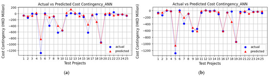
Figure 2.
Comparison of testing results for cost and contingency prediction: before and after integrating complexity index. (a) Prediction of materialized cost contingency before integrating complexity index. (b) Prediction of materialized cost contingency after integrating complexity index.
Further analysis was conducted to ascertain the importance of individual features to the ANN model’s predictive performance, utilizing permutation feature importance as defined in Equation (6). The analyses presented in Table 6 and Figure 3 indicate the significant role of the complexity index in improving the accuracy of the contingency prediction model. As Table 7 shows, the three most influential features affecting the cost prediction were approved PE, complexity index, and contract contingency. These findings align with the existing research, emphasizing the vital role of cost estimates [35] and contract contingencies [64] in project cost predictions. The results also emphasize the substantial impact of project complexity on contingency models, reinforcing the value of integrating a complexity index into future predictive models to improve their estimation accuracy. Furthermore, construction time-related variables, particularly the project start year, significantly influenced cost contingency predictions, while project type ranked fifth in importance (see Figure 3).
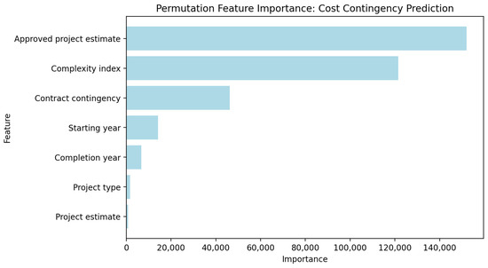
Figure 3.
Results of permutation feature importance.
Table 7.
Permutation feature results.
4.4. Integrating the Complexity Index into Interval Estimation
According to the methods outlined in Stage 4, interval prediction models were developed and evaluated with and without an integrated complexity index to achieve Objective 3.
Monte Carlo dropout and bootstrapping were employed to generate interval predictions for project cost and contingency; these results are illustrated in Figure 4 and Figure 5, respectively. Table 8 summarizes the uncertainty accuracy of the two approaches. The performance of the Monte Carlo dropout methods, which yielded narrower intervals, showed less accuracy, with uncertainty accuracy values of 60% for contingency prediction. Bootstrapping achieved a higher uncertainty accuracy (80%) by capturing a wider range of uncertainty. This difference is visually evident in Figure 4a and Figure 5a. The comparative analysis suggests that the narrower intervals produced by Monte Carlo dropout may have contributed to its lower prediction accuracy. While Monte Carlo dropout provides more precise estimates, its limited ability to capture a wider range of uncertainty may result in underestimating cost variability. On the other hand, bootstrapping’s broader intervals allow for a more comprehensive representation of uncertainty, which translates into improved predictive reliability.
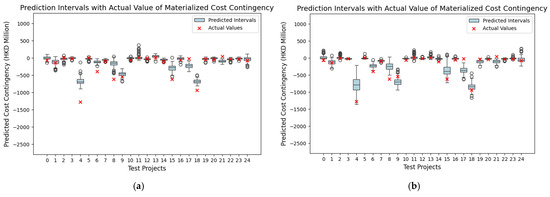
Figure 4.
Comparison of testing results of interval predictions using Monte Carlo dropout: before and after integrating complexity index. (a) Contingency interval predictions before integrating complexity index. (b) Contingency interval predictions after integrating complexity index.

Figure 5.
Comparison of testing results of interval predictions using bootstrapping: before and after integrating complexity index. (a) Contingency interval predictions before integrating complexity index. (b) Contingency interval predictions after integrating complexity index.
Table 8.
Comparison of ANN interval estimation: before and after integrating complexity index.
The subsequent integration of the complexity index markedly improved the performance of interval predictions for both the Monte Carlo dropout and bootstrapping approaches. Specifically, the uncertainty accuracy of cost interval predictions using Monte Carlo dropout increased by nearly 27%, rising from 60% to 76% (see Table 8). This improvement indicates that incorporating project complexity allows Monte Carlo dropout to better capture the underlying variability in cost and contingency estimations. As shown in Figure 4, a greater number of actual values fell within the predicted intervals post-integration, reinforcing the complexity index’s role in refining model performance. Similar improvements were observed in the bootstrapping models; the uncertainty accuracy of the interval predictions increased from 80% to 88% after incorporating the complexity index, as Table 8 shows. In addition, as illustrated in Figure 5b, this improvement signifies that the integration of the complexity index increased the alignment between the predicted intervals and actual data points, underscoring its effectiveness in refining the models’ predictive capability. Overall, these findings demonstrate that while bootstrapping provides a higher uncertainty accuracy, Monte Carlo dropout can yield competitive results when coupled with a complexity-based approach. The fact that integration of the complexity index improves the reliability of both interval predictions suggests that project complexity is a critical factor influencing cost contingency materialization.
5. Discussion
Cost contingency is a financial buffer that is allocated to address unforeseen expenses in a project and plays a pivotal role in risk management. The accurate estimation of cost contingency early in a project is essential for effective cost control and overall project success. Despite its importance, little research has explored the relationship between infrastructure-specific project characteristics and cost contingencies. Furthermore, studies that employ and compare multiple ML algorithms for contingency predictions using real-life datasets are sparse, and even fewer attempt interval estimates. Moreover, the influence of project complexity—a key determinant of cost performance—remains underexplored. This study seeks to close these research gaps by investigating how project characteristics and complexity contribute to both point and interval contingency estimates by leveraging multiple ML algorithms to improve prediction accuracy and reliability.
For point estimations, ANNs demonstrated the strongest predictive performance of the seven ML algorithms evaluated. An ANN’s ability to model complex, non-linear relationships likely accounts for its superior ability to capture the intricate associations between project characteristics and cost contingency, particularly in complex infrastructure projects. These findings align with the existing research on the topic. For example, Meharie [36] reported that ANNs outperformed linear regression and SVM in predicting costs for infrastructure projects, especially highway projects. Similarly, Wang et al. [35] found that ANNs surpassed four other ML algorithms (linear regression, SVM, decision trees, and random forests) in predictive accuracy. In this study, XGBoost ranked second in predictive performance. Elmousalami [9] previously concluded that XGBoost generally exhibits superior accuracy compared to other commonly used ML algorithms. These results suggest that both ANNs and XGBoost are well-suited for modeling contingency predictions and represent robust and reliable tools for academics and professionals addressing cost uncertainties in infrastructure projects.
Furthermore, a complexity index was introduced and integrated into both the point and interval contingency estimations. The complexity index captured key project factors to approximate project complexity through cost and duration. This method balances the trade-off between data availability and the need to encapsulate essential attributes of complexity, as the significance of project complexity in cost estimation has been emphasized in prior studies. Hatamleh et al. [45] demonstrated that increased complexity in supply chain decision-making reduces cost estimation accuracy. Similarly, Asmussen et al. [49] underscored the impact of project complexity on infrastructure cost estimations. In this study, integrating the complexity index significantly improved the ANN’s predictive performance, emphasizing the importance of incorporating a measure of complexity to improve infrastructure project cost estimation accuracy [47,49]. Feature importance analysis confirmed that the complexity index was a key variable affecting cost, ranking it as the second most influential factor and validating its importance for model robustness and predictive reliability.
This study also explored interval estimates for contingency predictions through two techniques: Monte Carlo dropout and bootstrapping. Both approaches offered the ability to operate without prior knowledge of the predictive distribution [38] and exhibited promising predictive performance. The results of these tests revealed an intriguing pattern. While bootstrapping offered superior overall accuracy, Monte Carlo dropout provided narrower prediction intervals, delivering a higher degree of precision in the resulting estimations. Vassilev et al. [42] also applied interval estimation techniques to semantic segmentation and reported that Monte Carlo dropout resulted in inferior classification accuracy compared to variational inference. Our study offers a plausible explanation for this lower uncertainty accuracy: the narrower intervals generated via Monte Carlo dropout likely contribute to its reduced accuracy. Therefore, for project planners seeking high uncertainty accuracy, bootstrapping would prove beneficial; for those seeking narrower intervals, Monte Carlo dropout may be preferable. Notably, integrating the complexity index into the interval estimates significantly improved both methods’ predictive performance, with Monte Carlo dropout showing particularly marked improvement. These findings underscore the value of the complexity index in achieving reliable infrastructure project cost contingency estimates.
In terms of practical implications, the demonstrated predictive power of ANNs and XGBoost presents a significant opportunity for industry adoption. Given their ability to capture complex, non-linear relationships between project characteristics and cost contingencies, these ML models provide a reliable alternative to traditional estimation methods. Construction firms and policymakers can leverage these models to enhance the accuracy of contingency forecasts. Second, the finding that project complexity significantly influences infrastructure cost contingency materialization is particularly relevant for project stakeholders. By incorporating the complexity index, they can better anticipate cost fluctuations and refine their budgetary strategies accordingly. Third, the introduction of interval predictions further enhances the decision-making process by offering project managers a probabilistic view of potential cost deviations. This added layer of uncertainty estimation is particularly valuable, as it facilitates proactive risk management by allowing project teams to assess worst-case and best-case scenarios. These findings suggest that bootstrapping is preferable for those prioritizing uncertainty accuracy, while Monte Carlo dropout demonstrates notable potential when integrated with the complexity index. This distinction allows practitioners to tailor their approach based on specific project characteristics and their risk tolerance.
6. Conclusions
This study improves cost contingency estimation for infrastructure projects by incorporating project-specific characteristics and a complexity index into both point and interval estimates. Among the seven ML algorithms tested, the ANN stood out as having the highest predictive accuracy for point estimates, achieving an R2 of 0.808. The inclusion of a complexity index constructed from cost and duration data significantly improved the ANN’s performance, increasing its R2 to 0.899 from 0.808. For interval estimates, bootstrapping more accurately represented uncertainty, while Monte Carlo dropout produced narrower prediction intervals. The complexity index notably boosted interval prediction performance, improving the uncertainty accuracy by 27% in Monte Carlo dropout and 10% in bootstrapping.
Theoretically, this study advances cost contingency estimation techniques by applying ML to project cost management and comparing multiple algorithms’ performance. It highlights the importance of including a complexity index, especially in highly complex infrastructure projects, and extends contingency prediction to interval estimates. These improvements help provide a deeper understanding of project cost risks and offer project managers valuable confidence ranges to better manage cost uncertainties.
Practically, practitioners can leverage the novel ANN-based model to enhance infrastructure cost planning and improve project delivery. The high predictive accuracy of ANNs positions them as a viable tool for practitioners conducting cost contingency estimations. Refined interval predictions equip project managers with better foresight into potential cost variances, enabling proactive cost management. For a new infrastructure project, key parameters such as project type, PEs, approved PEs, contract contingency, and planned duration can be readily obtained. Using these features, practitioners can quickly and accurately estimate a reasonable cost contingency, streamlining decision-making and reducing budget uncertainties. In summary, the ANN-based model offers a robust and efficient approach to cost estimation, equipping industry professionals with data-driven insights to enhance cost resilience and infrastructure project performance.
This study’s limitations include using a small dataset, which may restrict the generalizability of the results. A more extensive dataset could improve the model’s applicability across diverse project scenarios, as its predictive performance may vary in different contexts or larger-scale infrastructure developments. Future research could address this by using larger datasets to further validate the complexity index and enhance its robustness. In addition, the models used only six input variables due to data limitations. Future studies could improve the accuracy and robustness of their results by incorporating more variables. Moreover, cost contingency values were derived indirectly rather than from direct project records; future research should utilize actual cost contingency data to improve validity. Finally, the study focuses on infrastructure projects within a single geographical region, i.e., Hong Kong. Future research should explore the model’s performance in different geographical contexts to assess its broader applicability.
Author Contributions
Conceptualization, M.C.P.S. and Q.M.; Data curation, M.C.P.S.; Formal analysis, Q.M.; Methodology, M.C.P.S., Q.M. and Q.G.; Validation, Q.G.; Writing—original draft, Q.M.; Writing—review and editing, M.C.P.S. and Q.G. All authors have read and agreed to the published version of the manuscript.
Funding
The research is supported by the PolyU BRE incentive scheme P0047727.
Institutional Review Board Statement
Not applicable.
Informed Consent Statement
Not applicable.
Data Availability Statement
The original contributions presented in the study are included in the article; further inquiries can be directed to the corresponding author.
Acknowledgments
The authors would like to thank the Development Bureau of the HKSAR for sharing real-life project records for this study.
Conflicts of Interest
The authors declare no conflicts of interest.
References
- Lhee, S.C.; Flood, I.; Issa, R.R.A. Development of a two-step neural network-based model to predict construction cost contingency. J. Inf. Technol. Constr. 2014, 19, 399–411. [Google Scholar]
- Hoseini, E.; Bosch-Rekveldt, M.; Hertogh, M. Cost contingency and cost evolvement of construction projects in the preconstruction phase. J. Constr. Eng. Manag. 2020, 146, 5020006. [Google Scholar]
- Hammad, M.W.; Abbasi, A.; Ryan, M.J. Allocation and Management of Cost Contingency in Projects. J. Manag. Eng. 2016, 32, 04016014. [Google Scholar]
- Enshassi, A.; Ayyash, A. Factors affecting cost contingency in the construction industry–Contractors’ perspective. Int. J. Constr. Manag. 2014, 14, 191–208. [Google Scholar]
- Islam, M.S.; Prasad, M.; Skitmore, M.; Drogemuller, R. Automation in Construction Risk induced contingency cost modeling for power plant projects. Autom. Constr. 2021, 123, 103519. [Google Scholar] [CrossRef]
- Cardebat, J.-M.; Figuet, J.-M.; Paroissien, E. Expert opinion and Bordeaux wine prices: An attempt to correct biases in subjective judgments. J. Wine Econ. 2014, 9, 282–303. [Google Scholar]
- Lu, Y.; Luo, L.; Wang, H.; Le, Y.; Shi, Q. Measurement model of project complexity for large-scale projects from task and organization perspective. Int. J. Proj. Manag. 2015, 33, 610–622. [Google Scholar]
- Lin, W.; Wang, G.; Ning, Y.; Ma, Q.; Dai, S. The effects of performance measurement on megaproject performance: The moderating effects of project complexity. Eng. Constr. Archit. Manag. 2025, 32, 172–193. [Google Scholar]
- Elmousalami, H.H. Artificial intelligence and parametric construction cost estimate modeling: State-of-the-art review. J. Constr. Eng. Manag. 2020, 146, 3119008. [Google Scholar]
- El-Kholy, A.M.; Tahwia, A.M.; Elsayed, M.M. Prediction of simulated cost contingency for steel reinforcement in building projects: ANN versus regression-based models. Int. J. Constr. Manag. 2022, 22, 1675–1689. [Google Scholar]
- Ammar, T.; Abdel-Monem, M.; El-Dash, K. Regression-based model predicting cost contingencies for road network projects. Int. J. Constr. Manag. 2024, 1–15. [Google Scholar] [CrossRef]
- Han, Y.; Yang, Q.; Tian, P. The fundamentals of boosting high-quality development by megaprojects: A systematic literature review. Proj. Leadersh. Soc. 2024, 5, 100140. [Google Scholar]
- Flyvbjerg, B. What you should know about megaprojects and why: An overview. Proj. Manag. J. 2014, 45, 6–19. [Google Scholar] [CrossRef]
- Luo, L.; He, Q.; Jaselskis, E.J.; Xie, J. Construction project complexity: Research trends and implications. J. Constr. Eng. Manag. 2017, 143, 4017019. [Google Scholar]
- Project Management Institute. Project Management Body of Knowledge (Pmbok® Guide); Project Management Institute: Newtown Square, PA, USA, 2021. [Google Scholar]
- Doyle, A.; Hughes, W. The influence of project complexity on estimating accuracy. In Proceedings of the 16th Annual ARCOM Conference, Glasgow, UK, 6–8 September 2000. [Google Scholar]
- Sonmez, R.; Ergin, A.; Birgonul, M.T. Quantiative methodology for determination of cost contingency in international projects. J. Manag. Eng. 2007, 23, 35–39. [Google Scholar]
- Calford, E.M. Uncertainty aversion in game theory: Experimental evidence. J. Econ. Behav. Organ. 2020, 176, 720–734. [Google Scholar]
- Gal, Y.; Ghahramani, Z. Dropout as a bayesian approximation: Representing model uncertainty in deep learning. In Proceedings of the International Conference on Machine Learning, New York, NY, USA, 19–24 June 2016; pp. 1050–1059. [Google Scholar]
- Bruce, P.; Bruce, A.; Gedeck, P. Practical Statistics for Data Scientists: 50+ Essential Concepts Using R and Python; O’Reilly Media: Sebastopol, CA, USA, 2020; ISBN 1492072915. [Google Scholar]
- Idrus, A.; Nuruddin, M.F.; Rohman, M.A. Expert Systems with Applications Development of project cost contingency estimation model using risk analysis and fuzzy expert system. Expert Syst. Appl. 2011, 38, 1501–1508. [Google Scholar] [CrossRef]
- Musa, M.M.; Zubairu, I.K.; Bala, K. Appraisal of the performance of contingency cost provision for building projects in Nigeria. ATBU J. Environ. Technol. 2011, 4, 41–48. [Google Scholar]
- Barraza, G.A.; Asce, M.; Bueno, R.A. Cost Contingency Management. J. Manag. Eng. 2007, 23, 140–146. [Google Scholar]
- Thal, A.E., Jr.; Cook, J.J.; Iii, E.D.W. Estimation of Cost Contingency for Air Force Construction Projects. J. Constr. Eng. Manag. 2010, 136, 1181–1188. [Google Scholar]
- Maulud, D.; Abdulazeez, A.M. A review on linear regression comprehensive in machine learning. J. Appl. Sci. Technol. Trends 2020, 1, 140–147. [Google Scholar]
- Khodabakhshian, A. Machine Learning for Risk Management in Construction Projects. Ph.D. Thesis, Politecnico di Milano, Milan, Italy, 2023. [Google Scholar]
- Sohrabi, H.; Noorzai, E. Risk-supported case-based reasoning approach for cost overrun estimation of water-related projects using machine learning. Eng. Constr. Archit. Manag. 2024, 31, 544–570. [Google Scholar]
- Darko, A.; Glushakova, I.; Boateng, E.B.; Chan, A.P.C. Using machine learning to improve cost and duration prediction accuracy in green building projects. J. Constr. Eng. Manag. 2023, 149, 4023061. [Google Scholar]
- Yun, J.; Ryu, K.R.; Ham, S. Spatial analysis leveraging machine learning and GIS of socio-geographic factors affecting cost overrun occurrence in roadway projects. Autom. Constr. 2022, 133, 104007. [Google Scholar] [CrossRef]
- Wang, R.; Asghari, V.; Hsu, S.-C.; Lee, C.-J.; Chen, J.-H. Detecting corporate misconduct through random forest in China’s construction industry. J. Clean. Prod. 2020, 268, 122266. [Google Scholar]
- Chakraborty, D.; Elhegazy, H.; Elzarka, H.; Gutierrez, L. A novel construction cost prediction model using hybrid natural and light gradient boosting. Adv. Eng. Inform. 2020, 46, 101201. [Google Scholar]
- Coffie, G.H.; Cudjoe, S.K.F. Using extreme gradient boosting (XGBoost) machine learning to predict construction cost overruns. Int. J. Constr. Manag. 2023, 24, 1742–1750. [Google Scholar]
- Matel, E.; Vahdatikhaki, F.; Hosseinyalamdary, S.; Evers, T.; Voordijk, H. An artificial neural network approach for cost estimation of engineering services. Int. J. Constr. Manag. 2022, 22, 1274–1287. [Google Scholar]
- Nabawy, M.; Gouda Mohamed, A. Risks assessment in the construction of infrastructure projects using artificial neural networks. Int. J. Constr. Manag. 2024, 24, 361–373. [Google Scholar]
- Wang, R.; Asghari, V.; Man, C.; Hsu, S.; Lee, C. Automation in Construction Assessing effects of economic factors on construction cost estimation using deep neural networks. Autom. Constr. 2022, 134, 104080. [Google Scholar] [CrossRef]
- Meharie, M.G.; Mengesha, W.J.; Gariy, Z.A.; Mutuku, R.N.N. Application of stacking ensemble machine learning algorithm in predicting the cost of highway construction projects. Eng. Constr. Archit. Manag. 2022, 29, 2836–2853. [Google Scholar]
- Hon, C.K.H.; Sun, C.; Xia, B.; Jimmieson, N.L.; Way, K.A.; Wu, P.P.-Y. Applications of Bayesian approaches in construction management research: A systematic review. Eng. Constr. Archit. Manag. 2022, 29, 2153–2182. [Google Scholar]
- Milanés-Hermosilla, D.; Trujillo Codorniú, R.; López-Baracaldo, R.; Sagaró-Zamora, R.; Delisle-Rodriguez, D.; Villarejo-Mayor, J.J.; Núñez-Álvarez, J.R. Monte Carlo dropout for uncertainty estimation and motor imagery classification. Sensors 2021, 21, 7241. [Google Scholar] [CrossRef] [PubMed]
- Wu, L.; Mohamed, E.; Jafari, P.; AbouRizk, S. Machine Learning–Based Bayesian Framework for Interval Estimate of Unsafe-Event Prediction in Construction. J. Constr. Eng. Manag. 2023, 149, 4023118. [Google Scholar]
- Vaysse, K.; Lagacherie, P. Using quantile regression forest to estimate uncertainty of digital soil mapping products. Geoderma 2017, 291, 55–64. [Google Scholar]
- Gondia, A.; Siam, A.; El-Dakhakhni, W.; Nassar, A.H. Machine learning algorithms for construction projects delay risk prediction. J. Constr. Eng. Manag. 2020, 146, 4019085. [Google Scholar]
- Vassilev, H.; Laska, M.; Blankenbach, J. Uncertainty-aware point cloud segmentation for infrastructure projects using Bayesian deep learning. Autom. Constr. 2024, 164, 105419. [Google Scholar]
- Vidal, L.; Marle, F. Understanding project complexity: Implications on project management. Kybernetes 2008, 37, 1094–1110. [Google Scholar] [CrossRef]
- Qazi, A.; Quigley, J.; Dickson, A.; Kirytopoulos, K. Project Complexity and Risk Management (ProCRiM): Towards modelling project complexity driven risk paths in construction projects. Int. J. Proj. Manag. 2016, 34, 1183–1198. [Google Scholar]
- Hatamleh, M.T.; Hiyassat, M.; Sweis, G.J.; Sweis, R.J. Factors affecting the accuracy of cost estimate: Case of Jordan. Eng. Constr. Archit. Manag. 2018, 25, 113–131. [Google Scholar]
- Boonstra, A.; Reezigt, C. A complexity framework for project management strategies. Proj. Manag. J. 2023, 54, 253–267. [Google Scholar]
- Floricel, S.; Michela, J.L.; Piperca, S. Complexity, uncertainty-reduction strategies, and project performance. Int. J. Proj. Manag. 2016, 34, 1360–1383. [Google Scholar]
- Chen, Y.; Ahiaga-Dagbui, D.D.; Thaheem, M.J.; Shrestha, A. Toward a deeper understanding of optimism bias and transport project cost overrun. Proj. Manag. J. 2023, 54, 561–578. [Google Scholar]
- Asmussen, J.N.; Kristensen, J.; Wæhrens, B.V. Cost estimation accuracy in supply chain design: The role of decision-making complexity and management attention. Int. J. Phys. Distrib. Logist. Manag. 2018, 48, 995–1019. [Google Scholar]
- Tsamardinos, I.; Greasidou, E.; Borboudakis, G. Bootstrapping the out-of-sample predictions for efficient and accurate cross-validation. Mach. Learn. 2018, 107, 1895–1922. [Google Scholar]
- Cismondi, F.; Fialho, A.S.; Vieira, S.M.; Reti, S.R.; Sousa, J.M.C.; Finkelstein, S.N. Missing data in medical databases: Impute, delete or classify? Artif. Intell. Med. 2013, 58, 63–72. [Google Scholar]
- Emmanuel, T.; Maupong, T.; Mpoeleng, D.; Semong, T.; Mphago, B.; Tabona, O. A survey on missing data in machine learning. J. Big Data 2021, 8, 140. [Google Scholar] [CrossRef]
- Pham, T.Q.D.; Le-Hong, T.; Tran, X. V Efficient estimation and optimization of building costs using machine learning. Int. J. Constr. Manag. 2023, 23, 909–921. [Google Scholar] [CrossRef]
- Hossain, R.; Timmer, D. Machine learning model optimization with hyper parameter tuning approach. Glob. J. Comput. Sci. Technol. D Neural Artif. Intell. 2021, 21, 31. [Google Scholar]
- Adnan, M.; Alarood, A.A.S.; Uddin, M.I.; ur Rehman, I. Utilizing grid search cross-validation with adaptive boosting for augmenting performance of machine learning models. PeerJ Comput. Sci. 2022, 8, e803. [Google Scholar]
- Belete, D.M.; Huchaiah, M.D. Grid search in hyperparameter optimization of machine learning models for prediction of HIV/AIDS test results. Int. J. Comput. Appl. 2022, 44, 875–886. [Google Scholar]
- AlKheder, S.; Al Otaibi, H.; Al Baghli, Z.; Al Ajmi, S.; Alkhedher, M. Analytic hierarchy process (AHP) assessment of Kuwait mega construction projects’ complexity. Eng. Constr. Archit. Manag. 2025, 32, 1903–1946. [Google Scholar]
- Nguyen, A.T.; Nguyen, L.D.; Le-Hoai, L.; Dang, C.N. Quantifying the complexity of transportation projects using the fuzzy analytic hierarchy process. Int. J. Proj. Manag. 2015, 33, 1364–1376. [Google Scholar]
- Altmann, A.; Toloşi, L.; Sander, O.; Lengauer, T. Permutation importance: A corrected feature importance measure. Bioinformatics 2010, 26, 1340–1347. [Google Scholar] [PubMed]
- Gürsoy, M.İ.; Alkan, A. Investigation of diabetes data with permutation feature importance based deep learning methods. Karadeniz Fen Bilim. Derg. 2022, 12, 916–930. [Google Scholar]
- Saraiva, S.V.; de Oliveira Carvalho, F.; Santos, C.A.G.; Barreto, L.C.; Freire, P.K. de M.M. Daily streamflow forecasting in Sobradinho Reservoir using machine learning models coupled with wavelet transform and bootstrapping. Appl. Soft Comput. 2021, 102, 107081. [Google Scholar]
- Miok, K.; Nguyen-Doan, D.; Zaharie, D.; Robnik-Šikonja, M. Generating data using Monte Carlo dropout. In Proceedings of the 2019 IEEE 15th International Conference on Intelligent Computer Communication and Processing (ICCP), Cluj-Napoca, Romania, 5–7 September 2019; IEEE: Piscataway, NJ, USA, 2019; pp. 509–515. [Google Scholar]
- Offei-Nyako, K.; Ohene Tham, L.C.; Bediako, M.; Adobor, C.D.; Oduro Asamoah, R. Deviations between contract sums and final accounts: The case of capital projects in Ghana. J. Constr. Eng. 2016, 2016, 2814126. [Google Scholar]
- De Marco, A.; Narbaev, T.; Ottaviani, F.M.; Vanhoucke, M. Influence of cost contingency management on project estimates at completion. Int. J. Constr. Manag. 2024, 24, 935–945. [Google Scholar]
Disclaimer/Publisher’s Note: The statements, opinions and data contained in all publications are solely those of the individual author(s) and contributor(s) and not of MDPI and/or the editor(s). MDPI and/or the editor(s) disclaim responsibility for any injury to people or property resulting from any ideas, methods, instructions or products referred to in the content. |
© 2025 by the authors. Licensee MDPI, Basel, Switzerland. This article is an open access article distributed under the terms and conditions of the Creative Commons Attribution (CC BY) license (https://creativecommons.org/licenses/by/4.0/).