Article

A Low-Carbon Scheduling Method for Container Intermodal Transport Using an Improved Grey Wolf–Harris Hawks Hybrid Algorithm

by
Meixian Jiang
1,
Shuying Lv
1,
Yuqiu Zhang
2,
Fan Wu
1,
Zhi Pei
1 and
Guanghua Wu
1,*
1
College of Mechanical Engineering, Zhejiang University of Technology, Hangzhou 310023, China
2
College of Biomedical Science and Engineering, National University of Singapore Suzhou Research Institute, Suzhou 215123, China
*
Author to whom correspondence should be addressed.
Appl. Sci. 2025, 15(9), 4698; https://doi.org/10.3390/app15094698
Submission received: 4 March 2025 / Revised: 22 April 2025 / Accepted: 23 April 2025 / Published: 24 April 2025
(This article belongs to the Special Issue Green Technologies and Applications)

Abstract

:
Container intermodal scheduling is critical for advancing low-carbon logistics within inland port systems. However, the scheduling process faces several challenges, including the complexity of coordinating transport modes and complying with carbon emission policies. To address these issues, this study proposes a multi-objective optimization model that simultaneously considers transportation cost, carbon emissions, and time efficiency under soft time window constraints. The model is solved using an improved grey wolf–Harris hawks hybrid algorithm (IGWOHHO). This algorithm enhances population diversity through Tent chaotic mapping, balances global exploration and local exploitation with adaptive weight adjustment, and improves solution quality by incorporating an elite retention strategy. Benchmark tests show that IGWOHHO outperforms several well-established metaheuristic algorithms in terms of convergence accuracy and robustness. A case study based on an intermodal transport network further demonstrates that adjusting the objective weights flexibly provides decision support under various scenarios, achieving a dynamic balance between cost, efficiency, and environmental impact. Additionally, the analysis reveals that appropriate carbon tax pricing can encourage the adoption of greener transport modes, promoting the sustainable development of multimodal logistics systems.

1. Introduction

Carbon emissions pose a significant global challenge that hinders sustainable development across various sectors. In response, many countries have set carbon neutrality targets and integrated low-carbon strategies into their national development frameworks. The transportation sector, being one of the largest contributors to greenhouse gas emissions, plays a crucial role in achieving carbon reduction targets. Moreover, global events, such as the COVID-19 pandemic, trade tensions, and the Russia–Ukraine conflict, have disrupted international supply chains. These disruptions have highlighted the need for logistics systems that are resilient, economically efficient, and environmentally sustainable. Container intermodal transport has emerged as a promising solution, integrating multiple transportation modes, such as roads, rail, and waterways. This approach enhances operational efficiency, reduces logistics costs, and lowers carbon emissions. However, scheduling such systems remains a complex task. It requires precise coordination among transport modes, adherence to time window constraints, and compliance with environmental regulations.
Inland ports, which function as key hubs linking seaports to hinterland regions, have significant potential to advance low-carbon logistics by enhancing container transport efficiency and enabling multimodal coordination. Figure 1 illustrates the change in cargo distribution before and after the establishment of inland ports. The establishment of inland ports improves port collection and distribution systems, reduces regional logistics costs, and promotes local economic development. Furthermore, Figure 2 presents the operational mechanism of container intermodal scheduling, which necessitates integrated planning across multiple transport modes. The goal is to optimize the allocation of logistics resources while balancing economic and environmental objectives.
The inland container intermodal scheduling problem is a complex combinatorial optimization task with multiple nonlinear objectives and operational constraints. Traditional optimization techniques, such as dynamic programming and linear programming, often fail to provide efficient solutions for large-scale and real-time problems. In contrast, metaheuristic algorithms have gained attention for their global search capabilities and flexibility. Among these, the grey wolf optimizer (GWO) and Harris hawks optimization (HHO) have shown promising results in solving complex multi-objective problems. However, GWO is prone to premature convergence due to its limited local exploitation, while HHO lacks robustness in global exploration.
Optimization algorithms have demonstrated their effectiveness across various domains. In the field of the Internet of Things, both arithmetic optimization and hybrid metaheuristic algorithms have been used to enhance service composition and security. For example, improved shuffled frog leaping algorithms that integrate chaos theory, reverse learning, and Gaussian mutation have outperformed conventional methods [1,2]. In logistics, hybrid strategies have led to significant improvements in cold-chain logistics, vehicle routing, and sustainable supply chain design. These strategies include the combination of a large neighborhood search with non-dominated sorting genetic algorithm II (NSGA-II), tabu search with GWO, and NSGA-II with multi-objective particle swarm optimization [3,4,5]. Furthermore, advanced variants, such as the firefly algorithm integrated with the spotted hyena optimizer and GWO enhanced with artificial bee colony operators, have improved convergence, route optimization, and fleet sizing in multi-objective scenarios [6,7,8].
Building on recent advances in hybrid optimization algorithms, this study addresses container intermodal scheduling within inland port systems under low-carbon constraints. A multi-objective optimization model is proposed, considering transportation cost, carbon emissions, and transport time. To solve this model, an improved grey wolf–Harris hawks hybrid algorithm (IGWOHHO) is developed. This algorithm integrates Tent chaotic initialization, adaptive weight adjustment, and elite perturbation strategies to enhance search diversity and improve convergence performance.
The main contributions of this study are threefold. First, it introduces a unified scheduling model that integrates economic, environmental, and temporal objectives under realistic constraints. Second, it proposes the IGWOHHO algorithm, which improves solution quality through coordinated hybrid search strategies. Third, it presents a case study that validates the model and algorithm, demonstrating notable reductions in cost and emissions and supporting flexible decision-making across different policy and preference settings.
The structure of this paper is organized as follows. Section 1 introduces the research motivation, emphasizing the challenges of low-carbon container intermodal scheduling and the need for advanced optimization approaches. Section 2 reviews the background and related literature, discussing existing optimization methods for multimodal transport scheduling and low-carbon logistics, identifying current limitations, and highlighting the research gap. Section 3 presents the proposed multi-objective scheduling model and provides details on the design of the IGWOHHO algorithm. Section 4 outlines the algorithm parameters, the benchmark test functions used to validate algorithm performance, and the case study data. Section 5 evaluates the performance of the proposed algorithm and analyzes its application to intermodal transport scheduling under various scenarios. Section 6 concludes this study and offers suggestions for future research directions.

2. Background and Related Works

Container intermodal transport plays a pivotal role in global logistics, significantly contributing to low-carbon development. Although it represents only 16% of global maritime cargo by weight, it accounts for nearly 60% of the value of international trade, highlighting its importance in global supply chains [9]. Shifts to more sustainable transport modes, such as rail and waterborne transport, have demonstrated measurable environmental benefits. For instance, the expansion of these modes, alongside the adoption of electric trucks at Shenzhen Yantian Port, has led to a reduction in carbon emissions [10]. The International Energy Agency’s 2023 report on CO2 emissions identifies the transport sector as the largest contributor to the global rise in carbon emissions, with an increase of 240 million tonnes, predominantly driven by road transport. Road transport accounts for 30% of global freight and 5% of energy-related carbon emissions [11,12]. In contrast, inland waterway transport exhibits superior energy efficiency, requiring only 17% of the energy used by road transport to carry the same freight volume, and consuming approximately half the energy of rail transport [13]. These trends highlight the potential of container intermodal transport to enhance energy efficiency, reduce emissions, and support the sustainable transformation of logistics systems.
Path optimization for container intermodal transport has been extensively studied, with early models primarily focusing on transport cost, cargo characteristics, and infrastructure constraints. Recent multimodal routing approaches increasingly incorporate both economic and environmental objectives to support sustainable logistics. To improve network efficiency and reduce operational losses, advanced models have introduced capacity constraints, multi-commodity flow formulations, and cold-chain logistics considerations [14,15,16]. Although transport cost remains the primary factor in decision-making, several extended models have incorporated elements such as vehicle capacity, spoilage rates, and time-based penalties to better reflect practical logistics conditions [17,18]. However, most existing models address these factors separately, lacking a unified framework that simultaneously integrates economic, operational, and environmental objectives. This limitation reduces their applicability to real-world logistics systems, where multiple interdependent constraints must be considered holistically.
Various optimization approaches have been explored for container intermodal transport, including heuristics, hybrid models, and simulation-based strategies. Heuristic techniques, such as approximate dynamic programming, have improved scheduling efficiency under stochastic demand conditions [19]. Hybrid frameworks combining robust and possibilistic programming have been developed to address sustainability goals while coping with parameter uncertainty [20,21]. Simulation models have been applied to represent complex operational dynamics, including underground container handling, thereby offering decision support under realistic operational constraints [22]. Moreover, the integration of particle swarm optimization with dynamic programming has enhanced network recovery strategies and improved system resilience against disruptions [23,24]. Despite these contributions, limited research has examined adaptive hybrid strategies that effectively integrate global and local search capabilities, which are critical for achieving high convergence accuracy and robustness in large-scale multi-objective optimization problems.
Time window constraints are fundamental in intermodal scheduling, with soft time windows offering greater flexibility than rigid constraints. Several studies have developed multi-objective models that incorporate elastic or mixed time windows to simultaneously optimize transport cost, travel time, and emissions [25,26]. Furthermore, reinforcement learning has been introduced to capture spatiotemporal dependencies and enhance solution robustness under varying conditions [27,28]. Nevertheless, limited efforts have been made to integrate soft time window penalties directly into a comprehensive scheduling objective, especially when cost, time, and environmental goals must be balanced concurrently. This creates a need for models that reflect more realistic time flexibility while supporting effective trade-offs among multiple performance indicators.
Environmental sustainability has become increasingly central to intermodal transport optimization, with carbon emissions frequently incorporated as key objectives or constraints. Mixed integer programming has been employed to evaluate carbon pricing strategies and their effects on emissions and profitability [29,30]. Robust optimization frameworks have addressed uncertainties in demand and policy, improving the stability of low-carbon solutions [31,32]. Several models incorporate service-level considerations, including customer satisfaction, alongside economic and environmental factors [33,34]. Carbon tax and cap-and-trade mechanisms significantly influence mode selection and cost effectiveness under varying policy scenarios [35,36,37]. In addition, regional constraints such as emission caps and congestion controls have been integrated into multimodal planning models to assess system-wide impacts [38]. Despite these efforts, carbon pricing is often treated as an external parameter, rather than an internalized variable within the objective function. This limits the ability of existing models to support cost-sensitive and adaptive low-carbon decision-making across transport modes.
Although previous research has primarily focused on cost reduction and network efficiency in intermodal scheduling, limited efforts have been made to integrate multiple performance objectives within a unified framework. In particular, the joint consideration of cost, time, and carbon emissions under soft time window and carbon tax constraints remains insufficiently addressed. To bridge this gap, this study incorporates time window penalty costs and carbon tax expenses into the total cost and proposes a multi-objective optimization model that simultaneously accounts for economic, temporal, and environmental goals. The model is solved using the IGWOHHO algorithm, which effectively balances global exploration and local exploitation. A case study is conducted to validate the proposed model and analyze the impact of carbon tax policies on intermodal scheduling decisions.

3. Proposed Methods

To address the complexity of container intermodal transport scheduling under low-carbon constraints, a multi-objective optimization model is proposed. This model simultaneously considers total cost, transport time, and carbon emissions, incorporating carbon tax pricing and penalties for soft time window violations. Given the model’s nonlinear characteristics and multi-objective structure, an enhanced solution approach based on the IGWOHHO algorithm is introduced to tackle the problem efficiently.

3.1. Container Multimodal Transport Model

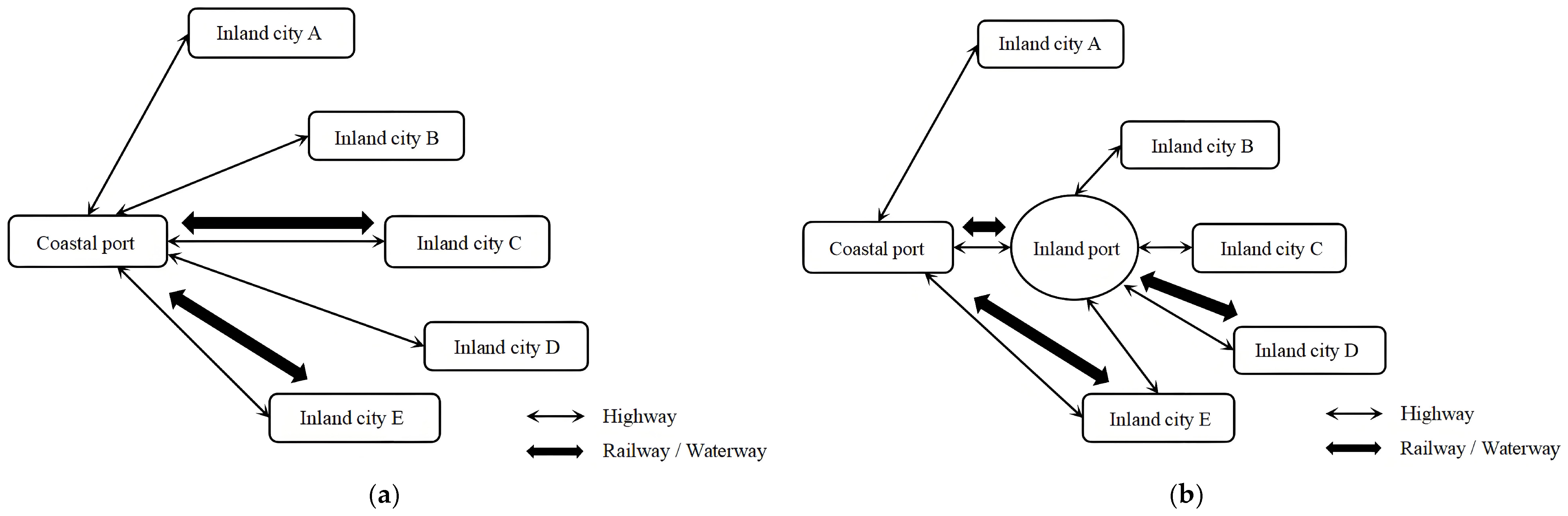
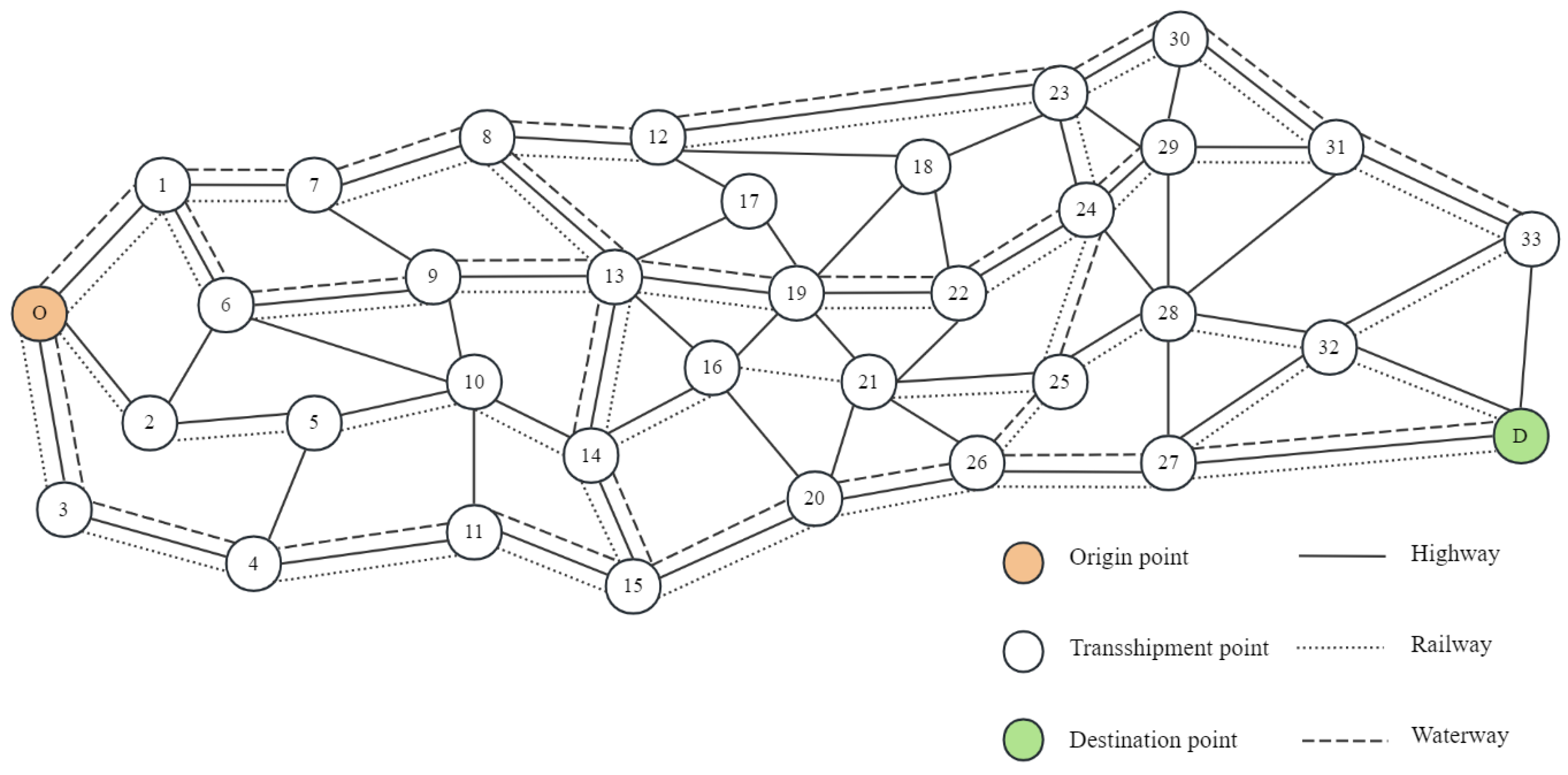
In intermodal container scheduling at inland ports, containers are typically transported directly from the yard to the railway yard or inland waterway terminal by road single-vehicle transport, without intermediate transshipment. To simplify cost calculation, this paper combines pickup and yard-to-yard operations into a single transshipment operation. Based on the actual scheduling process, the model divides the operation costs into three components, which include direct transport cost Cw, nodal transshipment cost Ct, and time penalty cost Cp. This categorization simplifies cost calculation, enhances the model’s practicality, and incorporates constraints related to transportation costs, time efficiency, and carbon emissions, thereby aligning more closely with the practical needs of multimodal transport scheduling optimization.
C w = i N j N k K q d i j k c i j k X i j k ,
C t = i N k N h K q c i k h Y i k h ,
C p = q s 1 i N m a x E i T i , 0 + q s 2 i N m a x T i L i , 0 .
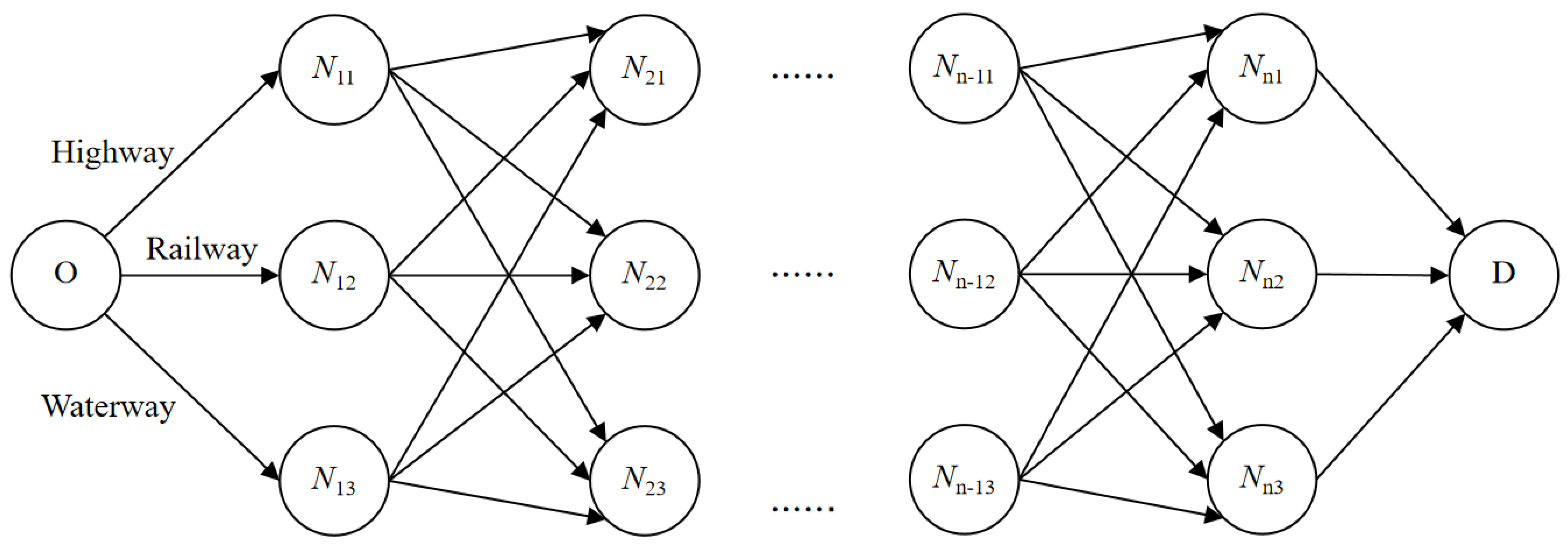
In this context, N represents the set of nodes, and K denotes the set of transport modes. The parameter q indicates the container demand, while d i j k and c i j k refer to the distance and per-unit cost between nodes i and j under mode k, respectively. The binary variable X i j k indicates whether mode k is selected between nodes i and j. The term c i k h denotes the per-unit transition cost from mode k to mode h at node i, with Y i k h representing the corresponding binary transition variable. The pair (Ei, Li) defines the soft time window bounds, Ti is the actual arrival time at node i, and s1 and s2 denote the unit penalty costs for early and late arrivals, respectively.
Carbon emissions E generated during intermodal transport arise from two primary sources. The first is fuel consumption by transport modes in operation, represented as Ef. The second source is the use of mechanized equipment in transshipment processes, represented as Em.
E f = i N j N k K q d i j k e k X i j k ,
E m = i N k K h K q f i k h Y i k h ,
where ek represents the unit carbon emission factor of mode k, and f i k h denotes the unit carbon emission factor associated with transitioning from mode k to h at node i.
In addition to mandatory carbon emission policies, a carbon tax is a key tool for promoting emission reductions by enterprises. By translating carbon emissions into economic costs through carbon tax pricing, the transition to low-carbon transportation can be effectively supported.
C c t = ρ E = ρ q i N j N k K d i j k e k X i j k + i N k K h K f i k h Y i k h ,
where ρ denotes the carbon tax rate. The expression incorporates both operational and transshipment-related emissions, converting them into monetary terms to reflect their economic impact within the scheduling model.
The total transport time T consists of two components. The first is the travel time of the transport vehicle Ts, which represents the duration of goods in transit. The second is the transit time at the transport node Tr, which reflects the efficiency of node operations.
T s = i N j N k K d i j k v k X i j k ,
T r = i N k K h K q t i k h Y i k h ,
where vk denotes the average speed of travel using the kth transport mode, and t i k h represents the transit time between nodes i and j for the selected kth mode.
Based on the above parameter definitions, this study constructs a container intermodal transport path optimization model for inland ports within a given planning period. Considering practical constraints related to cost, transport time windows, and carbon emissions, the objective function is defined as shown in Equation (9).
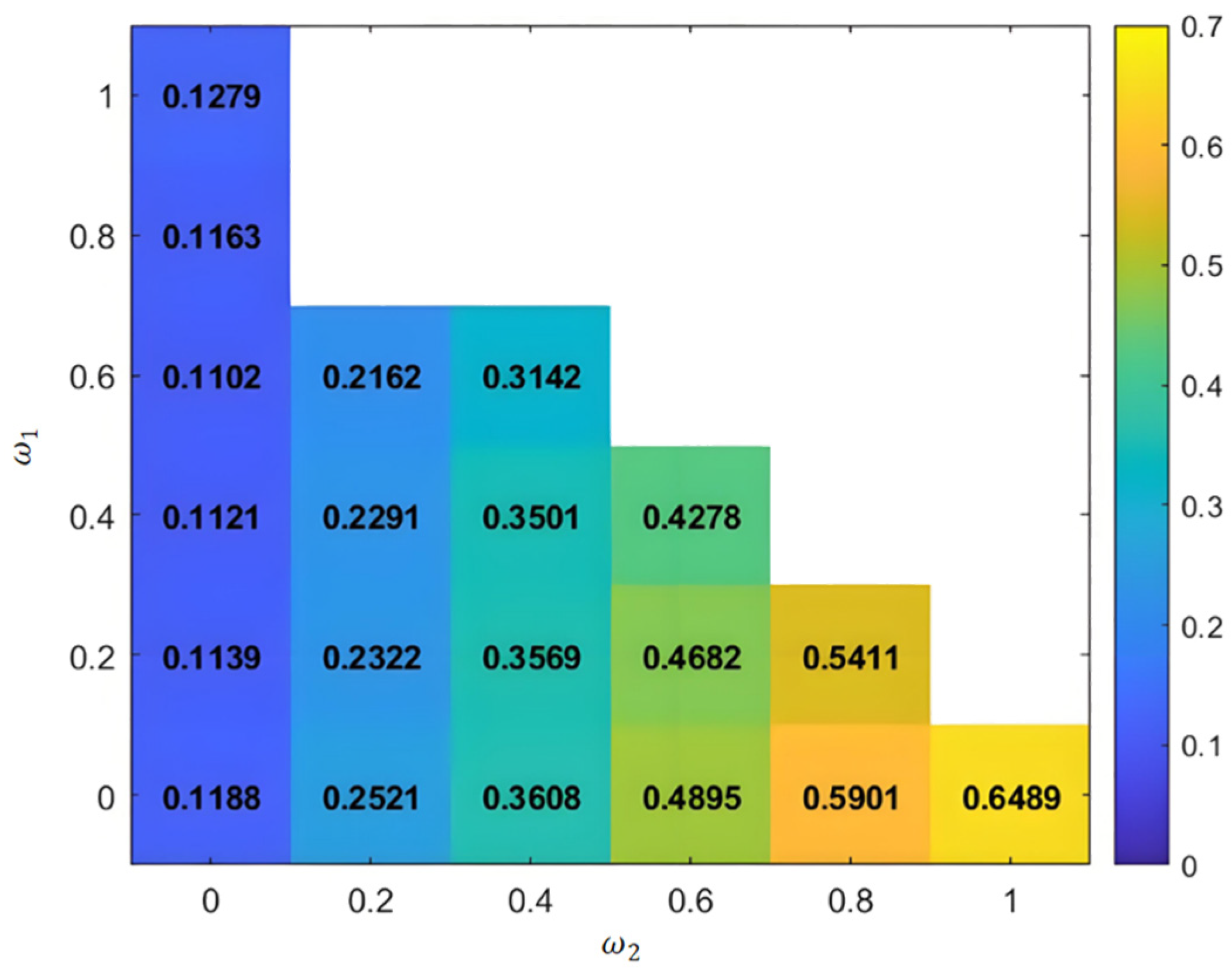
Z = ω 1 C + ω 2 T + ω 3 E = ω 1 C w + C t + C p + C c t + ω 2 T s + T r + ω 3 E f + E m ,
where ω1, ω2, and ω3 denote the weighting coefficients for total transport costs, transport time, and carbon emissions.
To ensure path uniqueness, the model restricts the selection to at most one transport mode between any two nodes, as specified in Equation (10).
k K X i j k 1                                                                   i , j N ,   k K .
The number of mode transitions per node is limited to one, as reflected in Equation (11), thereby avoiding multiple conversions between transport modes at the same node.
k K h K Y i k h 1                                           i N , k , h K , h k .
The coherence of transport modes is maintained by Equation (12), which ensures that if a mode transition occurs at node i, the inbound and outbound transport modes are logically consistent.
X i 1 , i k + X i , i + 1 k 2 Y i k h                                             i N , k , h K , h k .
No transport mode conversion is allowed at the origin or destination node, as specified in Equation (13).
Y o k h = Y d k h = 0                                                                               k , h K , h k .
The non-negativity and normalization of weight parameters are specified in Equation (14), which ensures that all weights range between 0 and 1 and their total equals one.
i = 1 3 ω i = 1 ,   0 ω i 1 .
To control emissions, Equation (15) limits total carbon emissions during the transport process, keeping them within the prescribed upper threshold.
E E m a x .
The arrival time of goods at node j is calculated based on the departure time from node i, the transition time, and the travel time, as shown in Equation (16).
T j = T i + q t i k h Y i k h + d i j k v k X i j k                                                               i , j N , k , h K , h k .  
The total transport time is constrained to remain within a predefined hard time window, as indicated in Equation (17).
T m i n T d = i N j N k K t i j k X i j k + i N k K h K t i k h Y i k h T m a x   i , j N , k , h K , h k .
The binary nature of the decision variables is specified in Equations (18) and (19), where both X i j k and Y i k h are restricted to values of 0 or 1.
X i j k 0 ,   1                                                                                                               i , j N , k K ,
Y i k h 0 ,   1                                                                                         i N , k , h K , h k .
The balance of cargo flow is maintained by Equation (20), which ensures that the inflow and outflow at each node remain equal throughout the scheduling process.
i , j N , k K X i j k i , j N , k K X j i k 1 ,                           j = d 0 , j N \ o , d 1 ,                     j = o                                               i , j N , k K .
The proposed model integrates soft time window constraints, alongside time penalty costs and carbon tax considerations, to balance the economic and environmental objectives. It includes a comprehensive set of constraints that guarantee the selection of feasible transport modes, compliance with time constraints, control of carbon emissions, and balance of flow. This approach establishes a strong foundation for optimizing intermodal transport scheduling with a focus on both cost efficiency and low-carbon objectives.

3.2. Multi-Objective Normalization and Weighted Aggregation

Since total cost, transport time, and carbon emissions differ in units and magnitudes, directly summing them may lead to biased optimization results. To ensure comparability and fairness in multi-objective scheduling, this study adopts a weighting approach. Each objective function is first normalized using a linear transformation to the range (0, 1). The multi-objective model is then converted into a single-objective formulation by assigning the weight coefficient ωi = 1 for one objective and ωj = 0 for others, minimizing total cost and transport time individually and determining the minimum carbon emissions by adjusting the corresponding weight. The maximum values of the remaining objectives are recorded as upper bounds for normalization. These reference values ensure consistent scaling of all objectives, preventing any single objective from dominating due to its larger magnitude. The objective function values are then transformed into dimensionless form using the max–min normalization method, as defined in Equation (21).
C = C i C i m i n C i m a x C i m i n , T = T i T i m i n T i m a x T i m i n , E = E i E i m i n E i m a x E i m i n ,  
where Ci, Ti, and Ei represent the original objective value. C i m i n , T i m i n , and E i m i n , along with C i m a x ,   T i m a x , and E i m a x , correspond to the minimum and maximum values obtained under single-objective optimization. The normalized dimensionless objective values, denoted as C , T , and E , fall within the range of (0, 1), indicating the relative deviation of the current solution from the optimal one.
A comprehensive evaluation of the objective function is performed by applying different weight combinations. The weighted objective function is constructed to calculate the overall evaluation value, as defined in Equation (22).
Z = ω 1 C + ω 2 T + ω 3 E .
Based on this, transport decisions are analyzed under various weighting schemes to assess the trade-offs between different objectives. By evaluating different weight combinations, the optimal scheduling solution is identified, considering factors such as cost efficiency, transport time, and carbon emissions. This analysis helps determine the most effective balance between these conflicting objectives, leading to an optimal low-carbon and cost-effective transport schedule.

3.3. Improved Grey Wolf–Harris Hawks Hybrid Algorithm

Proposed by Mirjalili et al. [39] in 2014, GWO is a heuristic algorithm inspired by grey wolf hunting behavior and social hierarchy. It solves complex optimization problems by simulating leadership structures and collaborative strategies within the wolf pack. The population is divided into α, β, δ, and ω, which correspond to the best, suboptimal, superior, and general solutions. The optimization process involves three main phases, including encircling the prey, tracking its position, and performing the attack.
In the encirclement phase, each individual estimates the distance to the prey using the distance vector D and updates its position by adjusting the step size based on the control coefficients A and C, thereby gradually approaching the optimal solution.
D = C · X p r e y t X t ,
X t + 1 = X p r e y t A · D ,
where X p r e y t represents the prey’s position, i.e., the current optimal solution at iteration t, while X t denotes the position of a grey wolf at the same iteration. T refers to the maximum number of iterations.
The adjustment coefficients A and C are determined by random variables r1 and r2, uniformly distributed within the range [0, 1], with their formulations provided in Equations (25) and (26).
A = 2 a · r 1 a ,
C = 2 r 2 .
The convergence factor a, which controls the magnitude of these coefficients, decreases linearly from 2 to 0 during the iteration process in accordance with Equation (27).
a = 2 2 t T .
In the position update phase, the general grey wolf generates candidate solutions X1, X2, and X3 by following the guidance of the three leading wolves, as illustrated in Equation (28).
D α = C 1 · X α X , X 1 = X α A · D α , D β = C 2 · X β X , X 2 = X β A · D β , D δ = C 3 · X δ X , X 3 = X δ A · D δ ,
where Xα, Xβ, and Xδ denote the positions of α, β, and δ wolves, which correspond to the top three solutions with the highest fitness. The distances of individual wolves from α, β, and δ head wolves are represented by Dα, Dβ, and Dδ, respectively. Additionally, C1, C2, and C3 are the random coefficients.
This process is further illustrated in Figure 3, which shows how the grey wolf updates its position based on the optimal, suboptimal, and superior solutions within the population.
The final position is calculated as a weighted average of the positions of the optimal, suboptimal, and superior individuals, guiding the population toward the optimal direction and enhancing convergence reliability, as presented in Equation (29).
X t + 1 = X 1 + X 2 + X 3 3 .
Due to its dynamic balance between global exploration and local exploitation, GWO is highly efficient for solving complex scheduling problems. Its simple structure, rapid convergence, and effective global search capability make GWO a powerful tool. It demonstrates strong robustness and fast convergence in multi-objective optimization and is widely applied in path planning, intelligent scheduling, and low-carbon logistics [40,41,42]. However, GWO tends to fall into local optima, particularly in high-dimensional problems, which limits its solution accuracy. The HHO algorithm addresses this issue by enhancing local search capabilities and improving adaptability in escaping local optima. Combining both algorithms enhances convergence stability and search performance for multi-objective scheduling problems.
Originally proposed by Heidari et al. [43] in 2019, the HHO algorithm is an emerging intelligent optimization method that has shown strong potential in logistics-related problems, such as the traveling salesman problem and vehicle routing [44,45]. Despite these promising results, its application in multimodal transport optimization remains limited and has not been systematically investigated in the literature.
During the exploration phase of the HHO algorithm, when |E| ≥ 1, the Harris hawk switches between two position update strategies depending on the value of q. If q ≥ 0.5, the hawk selects a random location within the population range for its next move. If q < 0.5, the hawk adjusts its position by considering the distance between the prey and the group’s central location. These two update strategies are presented in Equation (30), while Equation (31) defines the calculation of the group center.
X t + 1 = X r a n d t r 1 X r a n d t 2 r 2 X t                                       , X r a b b i t t X m t r 3 B 1 + r 4 B u B 1 ,       q 0.5 , q < 0.5 ,
X m t = 1 N i = 1 N X i t ,
where Xrand(t) represents the current position of a randomly selected individual, while Xrabbit(t) denotes the prey’s position. Xm(t) corresponds to the central position of the hawk flock, which is typically calculated as the average position of all the hawks in the population. This central position plays a guiding role in the HHO algorithm, allowing the hawks to coordinate their movements toward the prey during the optimization process. The set of random factors {ri|i = 1, 2, 3, 4} and q are values within the range (0, 1). Additionally, B1 and Bu define the upper and lower bounds of the parameters being optimized.
The escape energy E gradually decreases with the number of iterations, as formulated in Equation (32), reflecting the diminishing evasion capacity of the prey over time.
E = 2 E 0 1 t T ,
where E0 represents the initial random energy value within the range (−1, 1), t denotes the current iteration count, and T indicates the maximum number of iterations.
When |E| < 1, the HHO algorithm enters the exploitation phase and applies different hunting strategies based on the prey’s escape behavior. Under the soft encirclement condition, where |E| ≥ 0.5 and r ≥ 0.5, the hawks update their position according to the prey’s escape pattern.
X t + 1 = X t E J × X r a b b i t t X t ,
where X t represents the difference between the prey and hawk positions, and J denotes the jump distance during the rabbit’s escape process, as expressed in Equations (34) and (35).
X t = X r a b b i t t X t ,
J = 2 1 r 5 .
Upon satisfying the conditions |E| < 0.5 and r ≥ 0.5, the algorithm transitions into the hard encirclement phase, during which the hawks fixate on the prey, gradually reduce the search radius, and update their positions, as shown in Equation (36).
X t + 1 = X r a b b i t t E X t .
When |E| ≥ 0.5 and r < 0.5, the hawks either perform a high-speed dive to softly encircle the prey if it demonstrates strong escape ability or initiate Lévy flight behavior when predation fails. The updated position is expressed in Equation (37). The formulation of Lévy flight is provided in Equation (38).
X t + 1 = Y = X r a b b i t t E J × X r a b b i t t X t , Z = Y + S × L F D                                                                   ,     i f   F Y < F X t , i f   F Z < F X t ,  
L F X = 0.01 × u × σ v 1 β , σ = Γ 1 + β · sin π β 2 Γ 1 + β 2 · β · 2 β 1 2 1 / β ,  
where D represents the problem dimension, and S is a random vector of the same dimension. The variables u and v are random numbers uniformly distributed within the interval [0, 1]. The parameter β is a constant set to 1.5.
When the Lévy flight fails to yield an improved solution and the conditions |E| < 0.5 and r < 0.5 are satisfied, the algorithm enters the hard encirclement phase with high-speed swooping. In this stage, the hawks contract around the group center, and the position is updated using the following formulation as shown in Equation (39):
X t + 1 = Y = X r a b b i t t E J × X r a b b i t t X m t , Z = Y + S × L F D                                                                         ,     i f   F Y < F X t , i f   F Z < F X t .
In the original GWO-HHO hybrid optimization algorithm, GWO is primarily responsible for global exploration, while HHO focuses on local exploitation. However, the use of fixed weight assignment often leads to performance degradation and premature convergence. To address this issue and improve the balance between exploration and exploitation, this study proposes the IGWOHHO algorithm. The enhanced method integrates adaptive weighting, hybrid search, elite retention, and perturbation strategies to enhance search efficiency, convergence precision, and overall robustness.

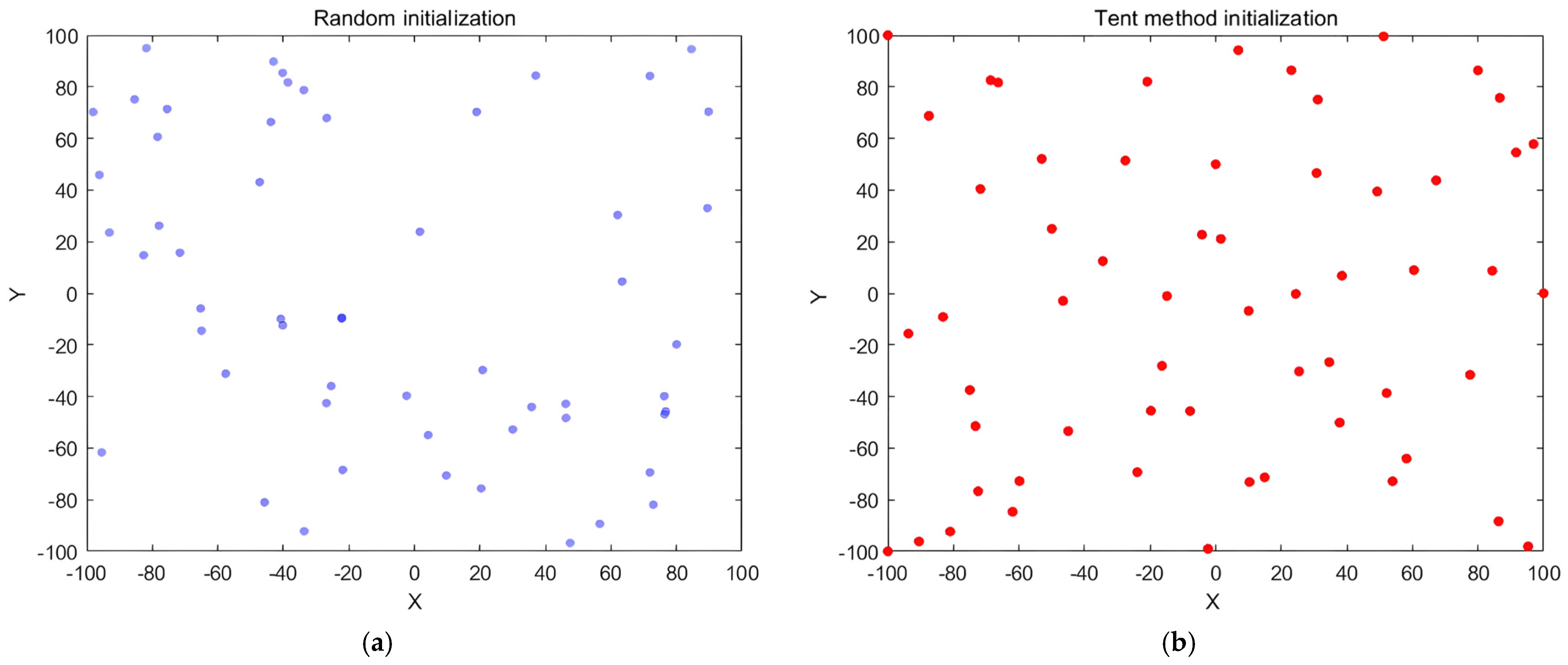
3.3.1. Tent Chaotic Mapping for Initial Population

At the initial stage of the algorithm, the Tent chaotic map is used to initialize the population, enhancing diversity and spatial coverage. As a representative chaotic mapping method, the Tent map exhibits strong traversal ability, uniform distribution, and dynamic complexity. These properties help avoid the clustering and sparsity issues often associated with random initialization, thereby improving the algorithm’s global search performance [46]. The mathematical expression of the Tent map used to generate the chaotic sequence is given in Equation (40).
z n + 1 = z n u                 ,     0 z n < 1 2 , 1 z n 1 u ,     1 2 z n 1 ,
where z n [ 0, 1] denotes the chaotic sequence of the nth generation. The initial value z o is typically generated randomly within the interval (0, 1). When u = 1 2 , the Tent map exhibits its most representative chaotic behavior.
Figure 4 compares the population distribution resulting from random initialization and Tent map-based initialization. The Tent mapping generates a more uniformly distributed sequence in the solution space, effectively reducing blind search regions and enhancing algorithmic robustness. This initialization approach provides a more favorable starting point for subsequent optimization.
The initial chaotic sequence zn, generated via the Tent map, is subsequently mapped into the problem domain [Xmin, Xmax] to construct the initial population X i 0 , as presented in Equation (41).
X i 0 = X m i n + X m a x X m i n × z n .

3.3.2. Convergence Factor and Flight Step Size Optimization

During the trapping phase of the GWO algorithm, the original implementation uses a linearly decreasing convergence factor a, as defined in Equation (27). However, this linear strategy may cause the search range to shrink prematurely in later iterations, reducing global exploration capability. To enhance search flexibility and avoid early convergence, this study introduces a stochastic disturbance based on the gamma distribution to adaptively adjust the convergence factor. The revised formulation is given in Equation (42).
a = 2 1 + e 0.025 t T 2 + ϑ · g a m r n d ,
where ϑ is the perturbation adjustment factor.
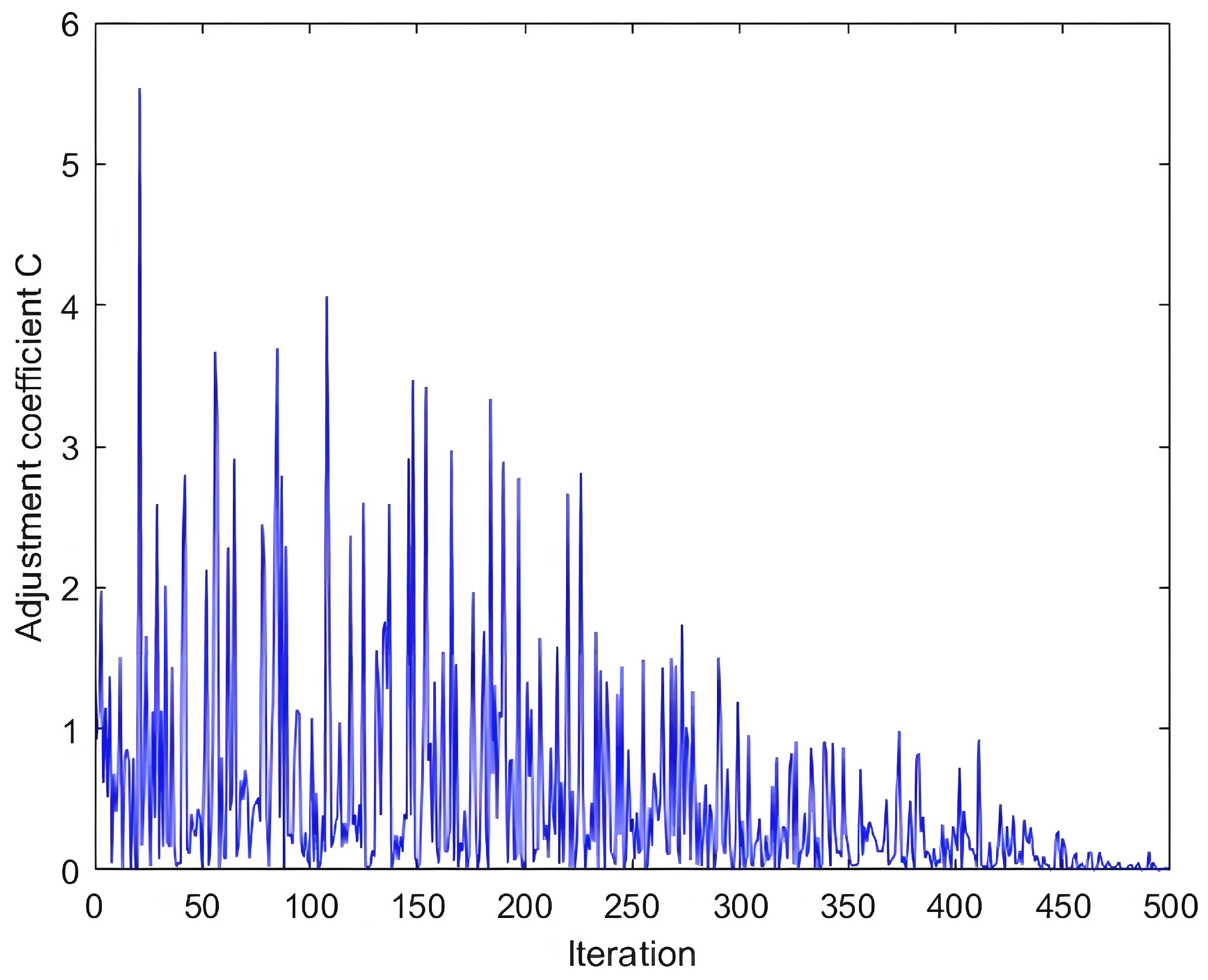
In addition, the adjustment coefficient C, which maintains stochastic fluctuations throughout the iteration process, does not fully capture the dynamic nature of the search phase. This limitation may lead to excessive dispersion during the early stage of the search. To address this issue, an adaptive convergence factor is introduced to refine the calculation of coefficient C in the GWO algorithm, as defined in Equation (43).
C = 4 r 1 μ , μ = 4 r 2 r 3 t T ,
where r 1 ,     r 2 ,     r 3 0 , 1 is a random factor used to improve search diversity.
Figure 5 illustrates that the dynamically adjusted value of coefficient C fluctuates significantly in the early stages, enhancing global exploration. As the iteration progresses, the value gradually stabilizes, supporting a balanced transition between exploration and exploitation.
The Lévy flight mechanism, proposed by the mathematician Paul Lévy, is a stochastic process characterized by a power-law distribution. In the local exploitation phase of the HHO algorithm, a fixed step size is typically used. In contrast, the original Lévy flight strategy introduces search jumps through randomly varying step sizes. Although its heavy-tailed distribution helps balance local intensification and global exploration, the step scaling factor is usually constant. This lack of adaptability may cause excessive variations in the search range during later iterations, which can undermine convergence stability and degrade solution quality. To address this issue, a dynamic step size adjustment mechanism is introduced. This allows the step length to gradually decrease with the iteration process, thereby adaptively controlling the search scope. The adjustment formulation is provided in Equation (44).
S = S 0 1 + β t T ,
where S0 is the initial step size and β controls the step contraction rate.
To further enhance search efficiency, each round of Lévy flights incorporates a dynamic step size adjustment. If the fitness of the newly generated solution does not surpass that of the current best solution, the search position is updated using a modified step size. When no improvement is observed over three consecutive iterations, a more refined local search is triggered to intensify exploitation.

3.3.3. Adaptive Weight Dynamic Switching Strategy

To enable adaptive adjustment and ensure a smooth transition during the search process, this study introduces a switching threshold, as defined in Equation (45).
ε t = ε m a x · e γ t T + ε m i n · 1 e γ t T ,
where the parameters   ε m a x and   ε m i n denote the maximum and minimum values of the switching threshold, respectively, and γ denotes the control parameter that regulates the rate of change. Preliminary experiments indicated that setting γ to 5 provides an optimal balance between exploration and exploitation. This setting enables the algorithm to effectively explore the search space while also converging to optimal or near-optimal solutions within a reasonable number of iterations.
To evaluate the search state in real time, the optimal solution change rate is introduced, as shown in Equation (46).
f = f b e s t t f b e s t t 1 f b e s t t 1 + η ,
where f b e s t t is the current optimal fitness, and η = 10−8 is added to avoid zero in the denominator.
If f   >   ε t , the search is still exhibiting significant improvement, and the GWO algorithm continues to guide global exploration. Conversely, when the change rate falls below the threshold, the solution tends to stabilize, and control is gradually shifted to the HHO algorithm to enhance local exploitation.
To prevent premature switching to the HHO algorithm caused by fluctuations in the optimal solution, the switching mechanism is further refined by introducing a weight ratio R t = λ H λ G as the dominant criterion. This mechanism dynamically adjusts the search weights of both algorithms based on the relationship between f and ε t , using a Sigmoid function as defined in Equation (47).
λ H t = 1 1 + e θ ε t f , λ G t = 1 λ H t ,
where θ is the sensitivity adjustment parameter, typically set to 10 [47].
Based on the dynamic changes in f and ε t , different switching conditions are defined for various search phases. In the early stage, a higher threshold allows larger solution fluctuations, promoting global exploration. In the middle stage, R t as the threshold gradually decreases to 1/2 R t 2.0, and the GWO and HHO algorithms cooperate to maintain a balance between exploration and exploitation. In the late stage, the threshold reaches its minimum while the improvement rate increases, allowing the HHO algorithm to dominate and enhance local search accuracy.
In the coordinated search phase, the GWO algorithm generates candidate solutions according to Equation (29), while the HHO algorithm selects appropriate position update strategies based on the prey escape energy E and the random factor r. The final position of each individual is then determined by a weighted combination of the two solutions, as defined in Equation (48).
X c o m b i n e d t = λ G t · X G W O t + λ H t · X H H O t .
However, the weighted combination is treated as a candidate solution rather than the final output. A multi-source selection mechanism is subsequently applied to determine whether the optimal solution should be updated, as defined in Equation (49).
X b e s t t = X G W O t           ,           i f   f G W O < f H H O f c o m b i n e d , X H H O t           ,           i f   f H H O < f G W O f c o m b i n e d , X c o m b i n e d t   ,             o t h e r w i s e .

3.3.4. Elite Retention and Perturbation Strategies

In population-based optimization algorithms, the elite retention strategy enhances convergence by preserving the best-performing individuals in each iteration, thereby preventing the loss of high-quality solutions [48]. However, relying solely on elite retention may reduce population diversity and increase the risk of premature convergence. To address this issue, a Gaussian stochastic perturbation mechanism is introduced to perform localized searches around elite individuals, thereby enhancing search diversity and improving global exploration capability.
After each iteration, individuals are ranked in descending order according to their fitness values, and the top P% are selected to form the elite set. To ensure retention of the current best solution X b e s t t , it is forcibly included in the elite set if it does not fall within the top P%. The elite set is defined in Equation (50).
X e l i t e t + 1 = X 1 , X 2 , . . . , X m X b e s t t , m = N × P .
To further enhance the exploration capability of elite individuals, Gaussian perturbation is introduced in Equation (51) to generate neighboring solutions. Building on this, Equation (52) incorporates a pair of sinusoidal functions to dynamically adjust the perturbation amplitude throughout the iteration process. In the early stage, a larger amplitude encourages broad exploration and reduces the risk of premature convergence. As the iteration progresses, the amplitude gradually decreases, enabling more focused local searches and improving solution refinement accuracy.
X e l i t e t + 1 = X e l i t e t + 1 + N 0 , σ 2 , σ = σ c × 1 t T × sin π t T ,
σ = σ c × 1 t T × sin π t T .
After each round of perturbation, the fitness of the newly generated neighboring solution is evaluated and compared with that of the original elite individual. The better-performing solution is retained for the next iteration, as defined in Equation (53).
X e n d e l i t e t + 1 = X e l i t e t + 1 ,     i f   f X e l i t e t + 1 < f X e n d e l i t e t , X e n d e l i t e t ,     o t h e r w i s e .                                                                                                      
During the hybrid search phase of the GWO and HHO algorithms, the fitness values of the combined candidate solutions and the elite-perturbed solutions are compared. The solution with the lowest fitness value is selected as the optimal one for the current iteration.
To maintain a constant population size, the updated elite and non-elite individuals after perturbation are merged and ranked in ascending order of fitness. The top N individuals are then selected to form the next generation. This merging process is expressed in Equation (54).
X n e w t + 1 = S e l e c t B e s t X e l i t e t X n o n e l i t e t , N ,
where   X n o n e l i t e t denotes the set of updated non-elite individuals, and the SelectBest function represents the selection of the top N optimal solutions based on fitness values to keep the population size constant.

3.3.5. Algorithm Execution Framework

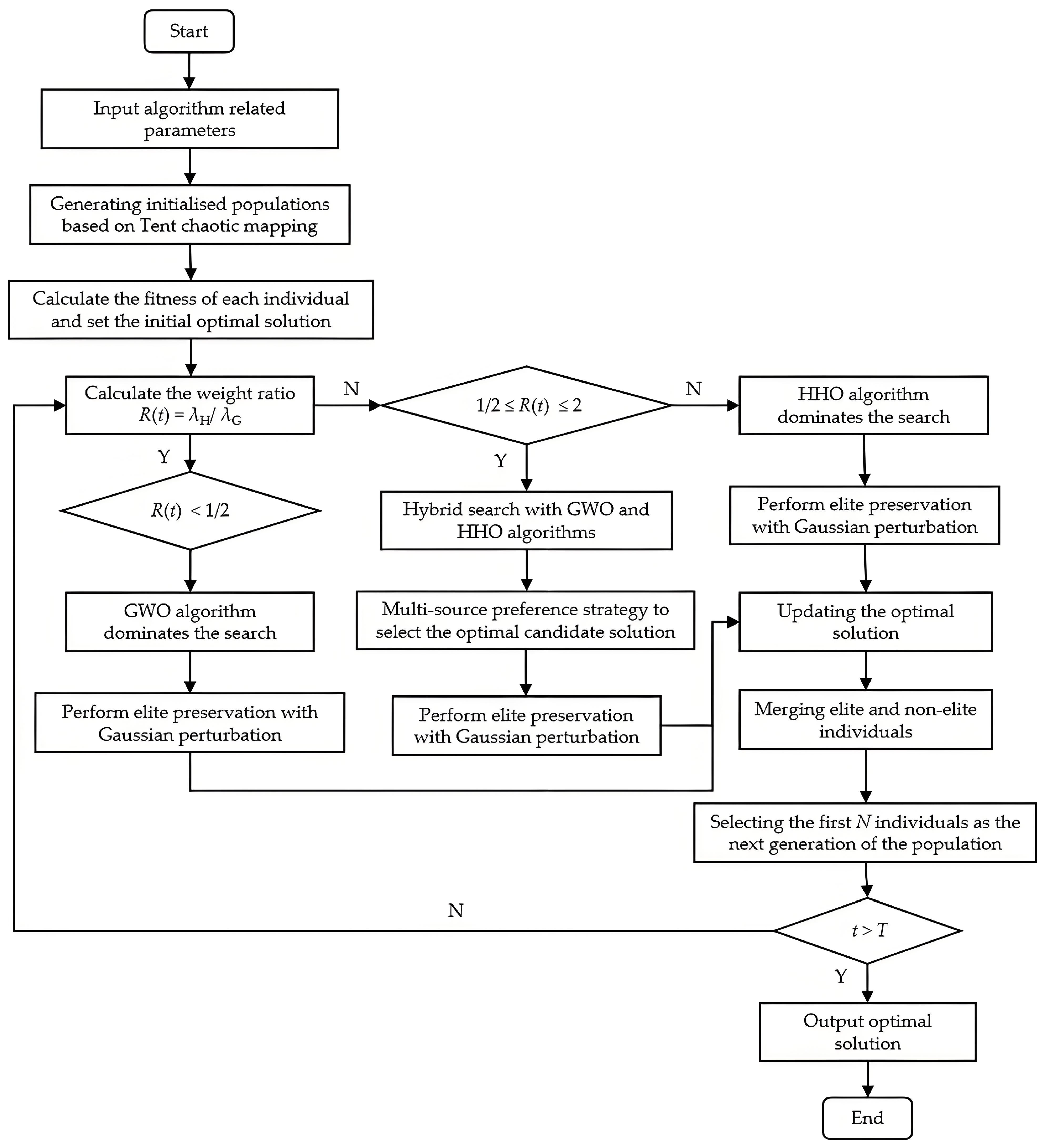
To systematically present the procedural logic of the proposed IGWOHHO algorithm, the pseudocode is provided in Algorithm 1, accompanied by a flowchart. These offer a clear and structured overview of the algorithm’s initialization, dynamic phase transition, hybrid search mechanism, and elite retention strategy.
Algorithm 1: Framework of the IGWOHHO algorithm
Input: population size N, max iterations T, perturbation adjustment coefficient ϑ , minimum switching threshold ε m i n , maximum switching threshold   ε m a x , elite retention ratio proportion P
Output: optimal solution X*
1: Initialize parameters N, T, ϑ ,   ε m i n ,   ε m a x , P
2: Generate initial population X0 using Tent chaotic mapping
3: Evaluate fitness of each individual in X0
4: Set the best individual as X*
5: for t = 1 to T do
6:   Evaluate fitness for all individuals
7:   Compute ε(t), change rate Δf(t), and dynamic weights λ_GWO, λ_HHO
8:   Compute ratio R(t) = λ_HHO/λ_GWO
9:   if R(t) < 0.5 then
10:     Perform the global search using GWO
11:     Apply elite retention and perturbation
12:     Update X* if better solution is found
13:   else if 0.5 ≤ R(t) ≤ 2.0 then
14:     Perform hybrid search
15:     Generate candidate solutions using both GWO and HHO
16:     Compute weighted combination
17:     Apply multi-source selection
18:     Apply elite retention and perturbation
19:     Update X* if a better solution is found
20:   else
21:     Perform local search using HHO based on E and r
22:     Apply Lévy-based dynamic refinement
23:     Apply elite retention and perturbation
24:     Update X* if a better solution is found
25:   end if
26:   Merge elite and non-elite groups, sort by fitness
27:   Select top N individuals for next generation
28: end for
29: return X*
Figure 6 presents the flowchart of the IGWOHHO algorithm, outlining the key steps from initialization to adaptive strategy selection and solution update. It illustrates the dynamic switching mechanism among GWO, HHO, and hybrid search phases.

4. Experimental Setup

This study was conducted in a Windows 10 environment with a hardware configuration of 16 GB RAM and an Intel Core i5-12400 CPU at 2.50 GHz. All algorithms were implemented and executed using MATLAB 2022b in Hangzhou.

4.1. Algorithm Parameter Settings

To enhance the performance of the IGWOHHO algorithm and ensure the robustness of its parameters, a sensitivity analysis was conducted on eight key parameters. Figure 7 illustrates the results using a heat map, where the color gradient ranges from black to white, with darker colors representing lower values and lighter colors corresponding to higher values. The analysis shows that the initial step size S0 has minimal impact on the objective function, indicating strong robustness, while the perturbation factor, switching thresholds, and elite retention ratio P exhibit greater sensitivity and require further tuning.
Since the algorithm’s performance tends to decline as the problem size increases, this study employed the Taguchi orthogonal design method to identify suitable parameter combinations through preliminary experiments. A signal-to-noise ratio (S/N ratio) analysis was performed using Minitab 19 software, and the main effect plot of the S/N ratio is presented in Figure 8. A higher S/N ratio indicates greater stability and improved solution quality.
Based on the analysis, the population size is set to 150, the maximum number of iterations to 500, the perturbation factor to 0.4, the minimum switching threshold to 0.025, the maximum switching threshold to 0.09, and the elite retention ratio to 0.08.

4.2. Benchmark Test Functions

To comprehensively evaluate the convergence behavior and global optimization performance of the proposed IGWOHHO algorithm, six representative benchmark functions were selected. Schwefel 2.22 and Rosenbrock are unimodal functions, used to assess the convergence speed and accuracy of the algorithm. Ackley and Penalized are multimodal functions characterized by complex landscapes with numerous local optima, making them suitable for testing global exploration capabilities. Foxholes and Kowalik are fixed-dimensional multimodal functions with intricate topologies, commonly used to evaluate local exploitation ability and solution stability. The definitions, dimensional settings, variable bounds, and known global optima for these benchmark functions are consistent with standard references in the literature [49,50], ensuring a reliable basis for performance comparison. The mathematical formulations are provided in Equations (55)–(60).
The Schwefel 2.22 function, defined in Equation (55), is a unimodal and separable test function that evaluates performance based on the combination of the sum and product of the absolute values of decision variables.
F 1 x = i = 1 n x i + i = 1 n x i ,
where x = (x1, x2, …, xn)∈[−10, 10]n, and the global minimum is 0, which occurs when xi = 0.
The Rosenbrock function, defined in Equation (56), is a unimodal and non-separable function characterized by a narrow, curved valley. It is commonly used to evaluate an algorithm’s convergence ability.
F 2 x = i = 1 n 1 100 x i + 1 x i 2 2 + x i 1 2 ,
where x∈[−30, 30]n, and the global minimum is 0, which occurs when xi = 1.
The Ackley function, defined in Equation (57), is a multimodal and non-separable function commonly used to evaluate global exploration capability in complex search spaces.
F 3 x = 20 e x p 0.2 1 n i = 1 n x i 2 e x p 1 n i = 1 n c o s 2 π x i + 20 + e ,
where x∈[−32, 32]n, and e is Euler’s number. The global optimum is 0.
The Penalized function, defined in Equation (58), incorporates penalty terms that increase the complexity of the optimization process, making it suitable for evaluating an algorithm’s robustness.
F 4 x = π n 10 s i n π y 1 + i = 1 n 1 y i 1 2 1 + 10 s i n 2 π y i + 1 + y n 1 2 + i = 1 n u x i , 10,100,4 ,
where yi = 1+ u(xi). The function introduces penalty terms for solutions outside the allowed region and has a global minimum value of 0 within the domain x∈[−50, 50]n.
The Foxholes function, defined in Equation (59), features a highly complex landscape with numerous local optima. It is commonly used to evaluate an algorithm’s ability to escape local optima and perform an effective global search.
F 5 x = 1 500 + j = 1 25 1 j + i = 1 2 x i a i j 6 1 ,
where x∈[−65, 65]2, and aij are constants define the positions of the holes in the landscape. The global minimum is approximately 0.998.
The Kowalik function, defined in Equation (60), is a low-dimensional multimodal function commonly used to evaluate local search accuracy and fine-tuning capability.
F 6 x = i = 1 11 a i x 1 b i 2 + b i x 1 b i 2 + b i x 3 + b i x 4 2 ,
where x = (x1, x2, …, xn)∈[−5, 5]4, and the parameters ai and bi are constants typically derived from empirical datasets. The global minimum is 0.
To illustrate the structural characteristics of the benchmark functions, Figure 9 presents three-dimensional plots that reveal key landscape features, including modality, convexity, basin depth, and the distribution of local optima. These visualizations facilitate the assessment of algorithm adaptability to both smooth and rugged search spaces. Comparing the landscapes clarifies the challenges posed by different objective functions. The plots also assist in analyzing algorithm behavior in flat regions, narrow valleys, and deceptive local minima, thereby enhancing the understanding of convergence dynamics and search efficiency.

4.3. Case Study Description

To evaluate the practical effectiveness of the proposed IGWOHHO algorithm, a case study is constructed based on a 35-node urban intermodal transport network. This case is adapted from the city arithmetic example network developed by Xiong and Wang [51], with further reference to the experimental framework used in multimodal transport scheduling optimization by Sun and Lang [52]. The network serves as a realistic and structured platform for validating the proposed model and algorithm.
The network structure is illustrated in Figure 10, reflecting an urban transport layout with multiple intermodal transfer possibilities. Between each pair of adjacent nodes, up to three transport modes are available in the fixed order of roads, rail, and inland waterways. Table 1 provides the transport distances for each mode and section. A blank entry indicates that a specific transport mode is not available for the corresponding segment.
The 35 nodes in the network consist of origin points, destination terminals, and intermediate transshipment hubs. Transport demand is defined for selected node pairs based on typical container flow patterns in inland logistics systems. Each node is associated with a soft time window, within which early or late arrivals are allowed but incur penalty costs. According to Table 2, soft time window constraints are applied to intermediate nodes, whereas a hard time window (25, 50) is enforced at the destination node D. The penalty cost is 100 CNY/TEU⋅h for early arrival and 200 CNY/TEU⋅h for delayed arrival.
The cargo is transported in standard containers, with each task involving the shipment of 40 TEUs from the origin to the destination. To enhance the model’s practical relevance, weighted average values of key parameters are adopted, reflecting actual conditions across different regions. For example, the International Carbon Price Floor policy establishes differentiated carbon prices based on economic development levels. The recommended rate is 75 USD/t CO2 for developed economies such as the United States, the European Union (EU), Canada, and the United Kingdom. For high-income emerging economies like China, the rate is 50 USD/t CO2, while for low-income developing countries like India, it is 25 USD/t CO2. Accordingly, this study adopts a carbon tax rate of 0.25 CNY/kg CO2.
Data on transport modes and modal transfer costs are sourced from the China Logistics Yearbook 2023 and the relevant academic literature. Table 3 and Table 4 summarize the operational parameters for each transport mode, including the associated costs, time requirements, and carbon emissions during intermodal transfers. The model incorporates emissions from both transportation and mechanized transshipment, calculated using standardized fuel consumption coefficients.

5. Results and Discussion

The experimental results for the proposed IGWOHHO algorithm are presented. A time complexity analysis is conducted to assess computational efficiency. Benchmark test functions are then used to evaluate the algorithm’s convergence, global search ability, and robustness, with comparisons to multiple heuristic algorithms under identical conditions. Furthermore, a case study involving a 35-node intermodal transport network analyzes the model’s performance, focusing on total cost, transport time, and carbon emissions under various operational settings, and carbon tax policies.

5.1. Algorithm Performance Evaluation

To comprehensively evaluate the performance of the proposed IGWOHHO algorithm, this subsection presents both theoretical analysis and empirical validation. The time complexity is examined to assess computational efficiency, while convergence performance is investigated through simulation experiments to demonstrate solution accuracy and stability.

5.1.1. Time Complexity Analysis

With a population size of N, problem dimension d, and a maximum number of iterations T, the time complexity of the algorithm primarily stems from population initialization, dynamic search, and elite retention. During the initialization phase, N individuals are generated using Tent chaotic mapping, each with d dimensions, yielding a complexity of O N d . In the dynamic search phase, both GWO and HHO algorithms update individual positions per iteration, with a computational complexity of O N d . The elite retention and perturbation mechanism involves sorting and perturbing elite individuals, resulting in an approximate complexity of O N log N + P N d .
Thus, the total time complexity per iteration is O N d + N log N + P N d . Given that P and log N are relatively small, their impact can be neglected. Therefore, the overall time complexity of the algorithm across T iterations is O T N d . Compared with the standard GWO and HHO algorithms, the IGWOHHO algorithm introduces multiple improvement strategies without significantly increasing computational cost. It effectively enhances global search ability and convergence performance, making it suitable for high-dimensional and complex optimization problems.

5.1.2. Convergence Performance Analysis

The whale optimization algorithm (WOA) is recognized for its robust global search capability, which is inspired by the hunting behavior of whales. Its ability to explore large search spaces effectively makes it particularly suitable for complex optimization problems. The sparrow search algorithm (SSA) is known for its ability to balance exploration and exploitation, mimicking the social behavior of sparrows to dynamically adjust its search strategy. This flexibility allows SSA to navigate both global and local search spaces. The dung beetle optimization (DBO) algorithm excels in multi-objective optimization, leveraging the dung beetle’s behavior to find optimal solutions by focusing on diverse objective functions and handling conflicting goals. To evaluate the performance of the proposed IGWOHHO algorithm, six benchmark test functions were selected and compared with several swarm intelligence algorithms, including WOA, SSA, DBO, GWO, and HHO. All algorithms were implemented under identical computational conditions using MATLAB 2022b, with a population size of 150 and a maximum of 500 iterations. Each algorithm was independently executed 20 times to ensure statistical reliability.
Table 5 summarizes the comparative results across all benchmark functions. The optimal value represents the best solution obtained and is used to evaluate solution accuracy. The average value reflects the algorithm’s robustness across multiple runs, while the standard deviation indicates the stability of its convergence behavior.
The results indicate that, for the unimodal Schwefel 2.22 function, the IGWOHHO algorithm successfully reaches the theoretical optimum of zero and outperforms all other algorithms across all evaluation metrics. In the case of the multimodal Ackley function, IGWOHHO, along with SSA, DBO, and HHO, achieves the theoretical optimal value. However, IGWOHHO demonstrates superior average convergence and a lower standard deviation, indicating better consistency in performance. For the Penalized function, IGWOHHO exhibits a stronger ability to escape local optima while maintaining higher solution stability compared to other algorithms. Regarding the fixed-dimensional multimodal functions, Foxholes and Kowalik, IGWOHHO outperforms the other algorithms in both optimal and average values. This further confirms its overall advantage in tackling complex optimization problems.
To further assess the convergence efficiency of IGWOHHO, its performance is compared with several other swarm intelligence algorithms across six benchmark functions. The convergence curves in Figure 11 demonstrate that although both GWO and HHO exhibit effective search capabilities, they show slightly lower stability and adaptability to complex problem landscapes than IGWOHHO. In contrast, algorithms such as SSA, WOA, and DBO are more susceptible to premature convergence, tend to get trapped in local optima, and display larger fluctuations in accuracy, indicating weaker robustness.
The dynamic adjustment mechanism of the IGWOHHO algorithm is further analyzed through the exploration and exploitation distribution illustrated in Figure 12. For unimodal functions, local exploitation increases rapidly as the iterations progress, indicating the algorithm’s strong refinement capability. In contrast, for multimodal functions, the algorithm maintains a high level of global exploration during the early stages and transitions smoothly to local exploitation in later iterations. This behavior reflects a well-balanced and adaptive search strategy that effectively responds to different landscape characteristics.
The performance evaluation confirms that the IGWOHHO algorithm outperforms several swarm intelligence algorithms across various benchmark functions. It achieves high solution accuracy, strong robustness, and stable convergence in both unimodal and multimodal scenarios. The dynamic adjustment mechanism ensures a balanced exploration and exploitation process, enhancing adaptability to different problem landscapes. Moreover, the algorithm maintains a competitive time complexity, demonstrating efficiency without increasing computational cost.

5.2. Intermodal Scheduling Case Study

To evaluate the practical applicability of the proposed model and algorithm, a case study is conducted using a 35-node intermodal transport network, as detailed in Section 4.3. The IGWOHHO algorithm is employed to solve the multi-objective scheduling problem, with a focus on total cost, transport time, and carbon emissions. The analysis compares the scheduling results obtained from different algorithms, examines the influence of varying objective weights on optimization outcomes, and assesses the impact of carbon tax rates on scheduling decisions.

5.2.1. Scheduling Performance Comparison

The intermodal container scheduling model is solved using six algorithms. Each algorithm independently generates a complete transport scheme based on the same input data and parameter settings. In practical decision-making, cost is usually the primary concern. Environmental impact and time efficiency are considered secondary but remain important. Therefore, the objective weights for cost, time, and carbon emissions are set to 0.5, 0.25, and 0.25, respectively. The results are presented in Table 6. This includes the objective function values, detailed transport routes, and selected transport modes. In the table, a, b, and c represent highways, railways, and waterways, respectively. The corresponding computation times are also reported. Figure 13 illustrates the total cost, carbon emissions, and transport time associated with the solutions produced by each algorithm, providing a comprehensive comparison of scheduling performance.
Algorithm solving time is an important indicator of computational performance. While the IGWOHHO algorithm requires slightly more time than the SSA algorithm, it outperforms the original WOA and DBO algorithms in terms of solving speed. In terms of cost optimization, IGWOHHO achieves a reduction of over 12% in total cost compared to the GWO and HHO algorithms. Regarding carbon emissions, it reports the lowest total emissions, which are 42.1% lower than those of the DBO algorithm. These results highlight its environmental advantages. Overall, the IGWOHHO algorithm demonstrates well-balanced performance in economic efficiency, environmental sustainability, and computational cost. Its improved objective function value further confirms its effectiveness in solving multi-objective optimization problems.

5.2.2. Weighting Factors’ Impact on Decision-Making

Changes in the weight coefficients of the objective function can significantly affect transport decision outcomes. In this experiment, all initial parameters are kept constant, with only the weight coefficients varied. The IGWOHHO algorithm is executed ten times for each setting to determine the optimal solution that minimizes the objective value, with the results presented in Figure 14. A higher weight coefficient indicates a greater emphasis on minimizing the corresponding sub-objective. Different weight configurations lead to varying levels of total cost, carbon emissions, and transport time, reflecting distinct optimization priorities.
Among the results, three representative solutions with objective values of 0.2162, 0.2322, and 0.4682 are selected for further analysis. Table 7 provides the details of the corresponding transport schemes for these selected solutions. Figure 15 visualizes the comparative performance of these schemes, focusing on total cost, carbon emissions, and transport time. This comparison highlights the effects of different weight settings on the algorithm’s ability to balance cost efficiency, environmental sustainability, and time efficiency.
The analysis of the results in Table 7 and Figure 15 reveals that varying the weightings of the objective function leads to different transport schemes. When cost is prioritized, as in option 1, the total cost is minimized, but both transport time and carbon emissions increase. In contrast, option 3, which emphasizes environmental sustainability, reduces carbon emissions, though it results in higher costs and longer transport times. By examining the effects of objective function weighting on optimization outcomes, customized transportation strategies can be developed to support decision-makers with diverse priorities. Adjusting the weightings provides flexibility, allowing for a dynamic balance between cost efficiency and environmental sustainability. This approach offers decision support for multi-scenario intermodal transport scheduling.

5.2.3. Carbon Tax Rate Impact Analysis

Both academic research and international practices acknowledge that, alongside mandatory carbon emission regulations, carbon taxation plays a crucial role in incentivizing enterprises to manage their carbon emissions effectively. Based on the previously described network structure, Table 8 presents the input data for arithmetic examples of varying sizes, which serve as the basis for subsequent analysis. The influence of carbon tax fluctuations, gradually increasing from zero, on transport mode selection and carbon emissions is analyzed. The results are visualized in a line graph, with Figure 16 illustrating the impact of carbon tax on transport modes and associated costs.
The introduction of a carbon tax has significantly contributed to reducing CO2 emissions. As the tax rate increases from 0.05 CNY/kg to 1 CNY/kg, emissions decrease substantially. However, beyond a tax rate of 0.8 CNY/kg, emissions stabilize, indicating that the relationship between the carbon tax and emissions is not strictly linear. While higher carbon taxes tend to increase total costs, the reduction in emissions at elevated tax levels partially offsets these costs, leading to a decline in total costs after reaching a peak.
In terms of transport modes, higher carbon taxes encourage a shift from road transport to rail and waterway alternatives, promoting a transition to more sustainable logistics. When the tax is below 0.15 CNY/kg, road transport remains dominant and contributes the most to pollution. At the EU’s base rate of 0.35 CNY/kg, stricter carbon tax policies result in a greater adoption of low-carbon transport modes. A well-calibrated carbon tax can optimize transport structures and mitigate emissions, but excessively high rates may impose economic burdens. Thus, achieving a balance between environmental sustainability and cost efficiency is essential.

6. Conclusions

This study presents a multi-objective optimization model for low-carbon multimodal transport scheduling, considering transportation cost, transit time, and carbon emissions under carbon tax constraints. The model incorporates flexible time window control, enhancing its adaptability to real-world scheduling scenarios. To solve this complex optimization problem efficiently, we propose the IGWOHHO algorithm, which combines the global exploration capability of the GWO algorithm with the local exploitation strength of the HHO algorithm. Additionally, the algorithm uses Tent chaotic mapping to improve initial population diversity, adaptive dynamic weight switching to balance exploration and exploitation, and an elite retention–perturbation strategy to enhance solution quality and avoid local optima.
Extensive benchmark tests on six classical test functions show that IGWOHHO outperforms GWO, HHO, SSA, WOA, and DBO in terms of convergence accuracy, robustness, and solution stability. In a case study based on a 35-node multimodal transport network, the algorithm achieves the best objective value, reducing total transport cost and carbon emissions by approximately 11.8% and 18.7%, respectively. Sensitivity analysis of weight parameters reveals that decision-makers with different strategic preferences can derive optimal transport solutions, supporting diverse policy or enterprise objectives. Furthermore, carbon tax simulations show that a moderate increase in carbon pricing can encourage shifts toward rail and water transport, effectively reducing emissions while keeping costs within a manageable range.
Future research could explore dynamic elements such as uncertain demand, traffic congestion, equipment failures, and supply chain disruptions to improve model adaptability and robustness. Incorporating such elements would enable the scheduling framework to better respond to complex and time-varying logistics environments. Additionally, alternative multi-objective optimization methods, such as Pareto front solutions, fuzzy preference models, or goal programming, could better address flexible decision-making preferences in scenarios with multiple stakeholders. Future studies may also focus on inland port scheduling with operational constraints, such as berth availability, yard capacity, and container handling time. With the increasing use of clean energy vehicles, integrating electric or hydrogen-powered transport into multimodal routing could further reduce emissions. Furthermore, applying the IGWOHHO algorithm in real-world systems, supported by artificial intelligence, deep learning, and large-scale data platforms, could enable intelligent and adaptive logistics scheduling under dynamic conditions.

Author Contributions

Conceptualization, S.L. and M.J.; methodology, S.L.; software, S.L.; validation, S.L. and F.W.; formal analysis, S.L.; investigation, S.L.; resources, Y.Z.; data curation, S.L.; writing—original draft preparation, S.L.; writing—review and editing, M.J.; visualization, G.W.; supervision, M.J. and Z.P.; project administration, M.J.; funding acquisition, M.J. and Z.P. All authors have read and agreed to the published version of the manuscript.

Funding

This research was funded by the National Natural Science Foundation of China (Grant No. 72271222), the National Natural Science Foundation of China (Grant No. 51605442), and Zhejiang Provincial Natural Science Foundation of China (Grant No. LGN18G010002).

Institutional Review Board Statement

Not applicable.

Informed Consent Statement

Not applicable.

Data Availability Statement

The data presented in this study are available on request from the corresponding author. The data are not publicly available, because they relate to the data privacy of the project.

Conflicts of Interest

The authors declare no conflicts of interest.

References

  1. Milutinovic, N.; Gajevic, M.; Krstovic, J.; Petrovic, A.; Bacanin, N.; Antonijevic, M. Performance of arithmetic optimization algorithm for ELM tuning applied to iot security. In Proceedings of the 2022 30th Telecommunications Forum (TELFOR), Belgrade, Serbia, 15–16 November 2022; pp. 1–4. [Google Scholar] [CrossRef]
  2. Tang, Z.; Wu, Y.; Wang, J.; Ma, T. IoT service composition based on improved Shuffled Frog Leaping Algorithm. Heliyon 2024, 10, e28087. [Google Scholar] [CrossRef] [PubMed]
  3. Wu, K.; Lu, Z.J.; Bai, E. Optimization of cold chain logistics distribution path considering traffic condition and replenishment along the way. PLoS ONE 2025, 20, e0305982. [Google Scholar] [CrossRef]
  4. Zhang, H.; Yan, J.; Wang, L. Hybrid Tabu-Grey wolf optimizer algorithm for enhancing fresh cold-chain logistics distribution. PLoS ONE 2024, 19, e0306166. [Google Scholar] [CrossRef]
  5. Abbasi, S.; Mousavi, S.S.; Farbod, E.; Sorkhi, M.Y.; Parvin, M. Hybrid data mining and data-driven algorithms for a green logistics transportation network in the post-COVID era: A case study in the USA. Systs. Soft Comput. 2024, 6, 200156. [Google Scholar] [CrossRef]
  6. Almazroi, A.A.; Ayub, N. Hybrid algorithm-driven smart logistics optimization in iot-based cyber-physical systems. Comput. Mater. Contin. 2023, 77, 3921–3942. [Google Scholar] [CrossRef]
  7. Ahmad, I.; Qayum, F.; Rahman, S.U.; Srivastava, G. Using improved hybrid grey wolf algorithm based on artificial bee colony algorithm onlooker and scout bee operators for solving optimization problems. Int. J. Comput. Intell. Systs. 2024, 17, 111. [Google Scholar] [CrossRef]
  8. Jiang, J.; Yu, N.; Ye, J.P.; Bai, W. Vehicle logistics path optimization based on ant colony and particle hybrid algorithm. JPCS 2021, 1865, 042086. [Google Scholar] [CrossRef]
  9. Organisation for Economic Co-Operation and Development-European Union Intellectual Property Office. Misuse of Containerized Maritime Shipping in the Global Trade of Counterfeits; OECD Publishing: Paris, France, 2021. [Google Scholar]
  10. World Resources Institute. Research on the Potential for Low-Carbon Development in Container Port Collection and Distribution Systems: Insights from Shenzhen Port. Available online: https://wri.org.cn/research/Optimizing-container-ports-transportation-and-Distribution-systems-toward-a-low-carbon-future (accessed on 1 March 2025).
  11. International Energy Agency. CO2 Emissions in 2023. Available online: https://iea.blob.core.windows.net/assets/33e2badc-b839-4c18-84ce-f6387b3c008f/CO2Emissionsin2023.pdf (accessed on 2 March 2025).
  12. Peet, K.; Gota, S.; Huizenga, C.; Medimorec, N.; Enriquez, A.; Yiu, A.; Verheul, B.; Dalkmann, H.; Cardama, M. Transport and Climate Change: Global Status Report 2018. Available online: http://slocat.net/tcc-gsr (accessed on 2 March 2025).
  13. Inland Waterways. Available online: https://transport.ec.europa.eu/transport-modes/inland-waterways_en (accessed on 3 March 2025).
  14. Moccia, K.; Zbigniew, G.; Marcin, P. Telematics-electronic data interchange/EDI/in port transport logistics. J. Decis. Syst. 2020, 29, 879–895. [Google Scholar] [CrossRef]
  15. Shang, C.J.; Li, Z.W.; Wang, J.; Liu, G.L.; Du, X.D. Research on evaluation of port railway collection and transportation system. E3S Web Conf. 2021, 261, 03028. [Google Scholar] [CrossRef]
  16. Meng, X.R.; Sun, J.M.; Wang, H.N. Cost Analysis of Multimodal Transport on Refrigerated Container. IOP Conf. Ser. Earth Environ. Sci. 2021, 791, 012078. [Google Scholar] [CrossRef]
  17. Kurtuluş, E.; Çetin, I.B. Analysis of modal shift potential towards intermodal transportation in short-distance inland container transport. Transp. Policy 2020, 89, 24–37. [Google Scholar] [CrossRef]
  18. Wang, L.; Liu, G.J.; Ahmad, I. Cost optimization model design of fresh food cold chain system in the context of big data. Big Data Res. 2023, 35, 100417. [Google Scholar] [CrossRef]
  19. Rivera, A.E.P.; Mes, M.R.K. Anticipatory scheduling of synchromodal transport using approximate dynamic programming. Ann. Oper. Res. 2022, 1–35. [Google Scholar] [CrossRef]
  20. Rahiminia, S.; Mehrabi, A.; Jabbarzadeh, A.; Aghaee, M.P. A hybrid optimization approach for designing sustainable intermodal freight transport under mixed uncertainty. Socio-Econ. Plan. Sci. 2025, 98, 102146. [Google Scholar] [CrossRef]
  21. Aparicio, J.T.; Arsenio, E.; Henriques, R. Assessing robustness in multimodal transportation systems: A case study in Lisbon. Eur. Transp. Res. Rev. 2022, 14, 28. [Google Scholar] [CrossRef]
  22. Pan, Y.; Liang, C.; Dong, L. A two-stage model for an urban underground container transportation plan problem. Comput. Ind. Eng. 2019, 138, 106113. [Google Scholar] [CrossRef]
  23. Viridiana, L.R.; Angélica, C.R.; Jesús Emilio, M.M.; Marco, A.; Liñán, C. Rescue and relocation of benthic organisms during an urban-port development project: Port of Manzanillo, case study. Aquat. Conserv. 2020, 30, 426–465. [Google Scholar] [CrossRef]
  24. Zukhruf, F.; Frazila, R.B.; Burhani, J.T.; Prakoso, A.D.; Sahadewa, A.; Langit, J.S. Developing an integrated restoration model of multimodal transportation network. Transp. Res. D Transp. Environ. 2022, 110, 103413. [Google Scholar] [CrossRef]
  25. Li, L.; Zhang, Q.; Zhang, T.; Zou, Y.; Zhao, X. Optimum Route and Transport Mode Selection of Multimodal Transport with Time Window under Uncertain Conditions. Mathematics 2023, 11, 3244. [Google Scholar] [CrossRef]
  26. Xiao, H.; Gong, H.J.; Wang, X.K.; Hang, B. Routes Choice in the international intermodal networks under the soft time window. Wirel. Commun. Mob. Com. 2022, 2022, 3355883. [Google Scholar] [CrossRef]
  27. Gülmez, B.; Emmerich, M.; Fan, Y. Multi-objective Optimization for Green Delivery Routing Problems with Flexible Time Windows. Appl. Artif. Intell. 2024, 38, 2325302. [Google Scholar] [CrossRef]
  28. Yu, F.H.; Chen, M.J.; Xia, X.Y.; Zhu, D.P.; Peng, Q.; Deng, K.B. Logistics distribution route optimization with Time Windows based on Multi-Agent Deep Reinforcement learning. Int. J. Inf. Technol. Sys. Appr. 2024, 17, 1–23. [Google Scholar] [CrossRef]
  29. Majumdar, A.; Singh, S.P.; Jessica, J.; Agarwal, A. Network design for a decarbonised supply chain considering cap-and-trade policy of carbon emissions. Ann. Oper. Res. 2023, 1–35. [Google Scholar] [CrossRef]
  30. Chen, X.; Hu, X.; Liu, H. Low-carbon route optimization model for multimodal freight transport considering value and time attributes. Socio-Econ. Plan. Sci. 2024, 96, 102108. [Google Scholar] [CrossRef]
  31. Zhang, X.; Jin, F.Y.; Yuan, X.M.; Zhang, H.Y. Low-Carbon Multimodal Transportation Path Optimization under Dual Uncertainty of Demand and Time. Sustainability 2021, 15, 8180. [Google Scholar] [CrossRef]
  32. Liu, Z.; Zhou, S.; Liu, S. Optimization of Multimodal Transport Paths Considering a Low-Carbon Economy Under Uncertain Demand. Algorithms 2025, 18, 92. [Google Scholar] [CrossRef]
  33. Cui, T.; Shi, Y.; Wang, J.; Ding, R.J.; Li, J.Z.; Li, K. Practice of an improved many-objective route optimization algorithm in a multimodal transportation case under uncertain demand. Complex Intell. Syst. 2025, 11, 136. [Google Scholar] [CrossRef]
  34. Tao, Y.; Zhang, S.L.; Lin, C.H.; Lai, X.F. A bi-objective optimization for integrated truck operation and storage allocation considering traffic congestion in container terminals. Ocean Coast. Manag. 2022, 12, 106417. [Google Scholar] [CrossRef]
  35. Wu, C.; Zhang, Y.; Xiao, Y.; Mo, W.; Xiao, Y.; Wang, J. Optimization of Multimodal Paths for Oversize and Heavyweight Cargo under Different Carbon Pricing Policies. Sustainability 2024, 16, 6588. [Google Scholar] [CrossRef]
  36. Sun, Y.; Zhang, C.; Chen, A.; Sun, G. Modeling a Green and Reliable Intermodal Routing Problem for Food Grain Transportation Under Carbon Tax and Trading Regulations and Multi-Source Uncertainty. Systems 2024, 12, 547. [Google Scholar] [CrossRef]
  37. Wang, X.N.; Cui, Z.Y.; Liu, M.Z.; Wang, L.F. Research on the choice of multimodal transportation emission reduction schemes based on different carbon tax models. JPCS 2021, 1972, 012111. [Google Scholar] [CrossRef]
  38. Kilani, M.; Diop, N.; De Wolf, D. A Multimodal Transport Model to Evaluate Transport Policies in the North of France. Sustainability 2022, 14, 1535. [Google Scholar] [CrossRef]
  39. Mirjalili, S.; Mirjalili, S.M.; Lewis, A. Grey wolf optimizer. Adv. Eng. Softw. 2014, 69, 46–61. [Google Scholar] [CrossRef]
  40. Yang, J.; Yan, F.; Zhang, J.; Peng, C. Hybrid chaos game and grey wolf optimization algorithms for UAV path planning. Appl. Math. Model. 2025, 142, 115979. [Google Scholar] [CrossRef]
  41. Rajamoorthy, R.; Arunachalam, G.; Kasinathan, P.; Devendiran, R.; Ahmadi, P.; Pandiyan, S.; Muthusamy, S.; Panchal, H.; Kazem, H.A.; Sharma, P. A novel intelligent transport system charging scheduling for electric vehicles using grey wolf optimizer and sail fish optimization algorithms. Energy Sources Part A 2022, 44, 3555–3575. [Google Scholar] [CrossRef]
  42. Lu, Y.; Li, S. Green Transportation Model in Logistics Considering the Carbon Emissions Costs Based on Improved Grey Wolf Algorithm. Sustainability 2023, 15, 11090. [Google Scholar] [CrossRef]
  43. Heidari, A.A.; Mirjalili, S.; Faris, H.; Aljarah, I.; Mafarja, M.; Chen, H. Harris hawks optimization: Algorithm and applications. Future Gener. Comput. Syst. 2019, 97, 849–872. [Google Scholar] [CrossRef]
  44. Gharehchopogh, F.S.; Abdollahzadeh, B. An efficient harris hawk optimization algorithm for solving the travelling salesman problem. Clust. Comput. 2022, 25, 1981–2005. [Google Scholar] [CrossRef]
  45. Li, S.; Zhang, R.; Ding, Y.; Qin, X.; Han, Y.; Zhang, H. Multi-UAV path planning algorithm based on BINN-HHO. Sensors 2022, 22, 9786. [Google Scholar] [CrossRef]
  46. Qi, Y.; Jiang, A.; Gao, Y. A Gaussian convolutional optimization algorithm with tent chaotic mapping. Sci. Rep. 2024, 14, 31027. [Google Scholar] [CrossRef]
  47. Tu, B.; Wang, F.; Huo, Y.; Wang, X.T. A hybrid algorithm of grey wolf optimizer and harris hawks optimization for solving global optimization problems with improved convergence performance. Sci. Rep. 2023, 13, 22909. [Google Scholar] [CrossRef] [PubMed]
  48. Li, Z.; Li, G.S.; Bilal, M.; Liu, D.Q.; Huang, T.; Xu, X. Blockchain-assisted server placement with elitist preserved genetic algorithm in edge computing. IEEE Internet Things J. 2023, 10, 21401–21409. [Google Scholar] [CrossRef]
  49. Naser, M.Z.; Al-Bashiti, M.K.; Tapeh, A.T.; Eslamlou, A.D.; Naser, A.; Kodur, V.; Hawileh, R.A.; Abdalla, J.; Khodadadi, N.; Gandomi, A.H. A Review of 315 Benchmark and Test Functions for Machine Learning Optimization Algorithms and Metaheuristics with Mathematical and Visual Descriptions. arXiv 2024, arXiv:2406.09581. [Google Scholar]
  50. Sharma, P.; Raju, S. Metaheuristic optimization algorithms: A comprehensive overview and classification of benchmark test functions. Soft Comput. 2024, 28, 3123–3186. [Google Scholar] [CrossRef]
  51. Xiong, G.; Wang, Y. Best routes selection in multimodal networks using multi-objective genetic algorithm. J. Comb. Optim. 2014, 28, 655–673. [Google Scholar] [CrossRef]
  52. Sun, Y.; Lang, M. Bi-objective optimization for multi-modal transportation routing planning problem based on Pareto optimality. J. Ind. Eng. Manag. 2015, 8, 1195–1217. [Google Scholar] [CrossRef]
Figure 1. Impact of inland ports on cargo distribution in coastal ports. (a) Transport routes before inland port implementation; (b) transport routes after inland port implementation.
Applsci 15 04698 g001
Figure 2. Container loading scheduling process.
Applsci 15 04698 g002
Figure 3. The grey wolf location update in the grey wolf algorithm.
Applsci 15 04698 g003
Figure 4. Two methods for initializing the population distribution. (a) Random initialization; (b) Tent method initialization.
Applsci 15 04698 g004
Figure 5. Variation in adjustment coefficient C during the iteration process.
Applsci 15 04698 g005
Figure 6. Flowchart of the IGWOHHO algorithm.
Applsci 15 04698 g006
Figure 7. Sensitivity analysis of algorithm parameters.
Applsci 15 04698 g007
Figure 8. Main effect chart of S/N ratio for algorithm parameter evaluation.
Applsci 15 04698 g008
Figure 9. Three-dimensional graphs of functions. (a) Schwefel 2.22 function; (b) Rosenbrock function; (c) Ackley function; (d) Penalized function; (e) Foxholes function; (f) Kowalik function.
Applsci 15 04698 g009
Figure 10. Network structure of the arithmetic example.
Applsci 15 04698 g010
Figure 11. Convergence trends of algorithms on benchmark test functions. (a) Schwefel 2.22 function; (b) Rosenbrock function; (c) Ackley function; (d) Penalized function; (e) Foxholes function; (f) Kowalik function.
Applsci 15 04698 g011
Figure 12. Function exploitation and exploration progress. (a) Schwefel 2.22 function; (b) Rosenbrock function.
Applsci 15 04698 g012
Figure 13. Comparison of total cost, carbon emission, and time across algorithms.
Applsci 15 04698 g013
Figure 14. Optimal values with different weight coefficients.
Applsci 15 04698 g014
Figure 15. Targeted results of different programs.
Applsci 15 04698 g015
Figure 16. Impact of a carbon tax on transport modes and costs. (a) Changes in total costs and carbon emissions; (b) changes in the frequency of modes of transport.
Applsci 15 04698 g016
Table 1. Distance traveled by different modes of transport.
SectionsTransport DistanceSectionsTransport DistanceSectionsTransport Distance
O–1(110, 101, 129)12–18(103, —, —)22–24(133, 115, 142)
O–2(134, 164, —)12–23(128, 138, 132)23–24(133, 135, —)
O–3(75, 83, 107)13–14(143, 146, 146)23–29(150, —, —)
1–6(148, 161, 166)13–16(63, —, —)23–30(135, 145, 161)
1–7(120, 133, 112)13–17(107, —, —)24–25(94, 98, —)
2–5(103, 80, —)13–19(130, 136, 145)24–28(138, —, —)
2–6(85, —, —)14–15(103, 87, 111)24–29(146, 136, 153)
3–4(117, 125, 137)14–16(132, 141, —)25–26(73, —, 96)
4–5(75, —, —)15–20(100, 73, 114)25–28(107, 82, —)
4–11(150, 166, 173)16–19(129, —, —)26–27(132, 120, 150)
5–10(101, 86, —)16–20(81, —, —)27–28(137, —, —)
6–9(144, 167, 162)16–21(—, 80, —)27–32(110, 104, —)
6–10(133, —, —)17–19(67, —, —)27–D(117, 129, 143)
7–8(128, 119, 134)18–19(110, —, —)28–29(76, —, —)
7–9(105, —, —)18–22(76, —, —)28–31(130, —, —)
8–12(112, 84, 115)18–23(115, —, —)28–32(104, 96, —)
8–13(113, 112, 124)19–21(119, —, —)29–30(141, —, —)
9–10(126, —, —)19–22(125, 114, 138)29–31(129, 140, —)
9–13(135, 149, 140)20–21(95, —, —)30–31(95, 89, 118)
10–11(88, —, —)20–26(110, 97, 119)31–33(106, 106, 114)
10–14(120, 136, —)21–22(73, —, —)32–33(120, 125, —)
11–15(90, 74, 90)21–25(111, 89, —)32–D(117, 84, —)
12–17(55, —, —)21–26(65, —, —)33–D(108, —, —)
Table 2. Time windows for different nodes.
NodeSoft Time WindowNodeSoft Time WindowNodeSoft Time Window
1(1, 3)12(12, 19)23(26, 35)
2(1, 3)13(13, 20)24(27, 36)
3(2, 5)14(14, 23)25(28, 37)
4(3, 6)15(17, 25)26(28, 37)
5(3, 7)16(18, 27)27(30, 39)
6(4, 8)17(20, 29)28(31, 39)
7(4, 9)18(21, 30)29(32, 40)
8(5, 12)19(22, 33)30(34, 41)
9(7, 15)20(22, 33)31(34, 43)
10(8, 17)21(24, 34)32(36, 43)
11(10, 18)22(25, 35)33(36, 46)
Table 3. Data relating to the mode of transport.
SymbolHighwayRailwayWaterway
v k   k m · h 806525
c i j k   C N Y / k m · T E U 6.223.451.87
e k   k g / k m · T E U 0.890.160.32
Table 4. Data related to the modal shift in transport.
SymbolHighway–RailwayRailway–WaterwayWaterway–Highway
t i k h   h / T E U 0.140.200.26
c i k h   C N Y / T E U 150275200
f i k h   k g / T E U 2.161.891.95
Table 5. Algorithm optimization results.
FunctionEvaluation
Indicators
GWOSSAWOADBOHHOIGWOHHO
Schwefel 2.22Best4.80 × 10−241.82 × 10−2453.75 × 10−601.77 × 10−961.90 × 10−610
Mean1.19 × 10−233.14 × 10−2342.51 × 10−561.74 × 10−773.37 × 10−559.03 × 10−238
St.dev6.62 × 10−2405.02 × 10−563.89 × 10−777.32 × 10−550
RosenbrockBest2.56 × 1012.92 × 10−72.63 × 1012.41 × 1018.21 × 10−52.82 × 10⁻¹¹
Mean2.64 × 1012.94 × 10−12.66 × 1012.47 × 1014.17 × 10−42.05 × 10⁻⁶
St.dev6.52 × 10−13.01 × 10−62.84 × 10−14.24 × 10−13.43 × 10−43.17 × 10⁻¹⁰
AckleyBest2.58 × 10−148.88 × 10−168.88 × 10−168.88 × 10−168.88 × 10−168.88 × 10⁻¹⁶
Mean2.86 × 10−148.88 × 10−163.02 × 10−158.88 × 10−168.88 × 10−168.88 × 10⁻¹⁶
St.dev1.58 × 10−1503.18 × 10−15000
PenalizedBest6.57 × 10−32.45 × 10−133.02 × 10−47.26 × 10−162.55 × 10−117.25 × 10⁻¹⁶
Mean1.92 × 10−21.86 × 10−121.56 × 10−33.18 × 10−88.70 × 10−78.23 × 10−14
St.dev1.61 × 10−22.15 × 10−122.54 × 10−37.11 × 10−81.67 × 10−61.27 × 10−13
FoxholesBest9.98 × 10−19.98 × 10−19.98 × 10−19.98 × 10−19.98 × 10−19.98 × 10⁻¹
Mean3.33 × 1003.73 × 1009.98 × 10−19.98 × 10−11.20 × 1009.98 × 10−1
St.dev5.22 × 1005.07 × 1003.79 × 10−102.89 × 10−144.45 × 10⁻¹⁰
KowalikBest3.31 × 10−43.31 × 10−43.24 × 10−43.08 × 10−43.08 × 10−43.07 × 10⁻⁴
Mean3.07 × 10−43.08 × 10−48.20 × 10−48.07 × 10−44.96 × 10−43.07 × 10⁻⁴
St.dev2.54 × 10−94.58 × 10−84.30 × 10−44.32 × 10−44.07 × 10−42.05 × 10⁻¹²
Table 6. Solution results of different algorithms.
AlgorithmObjective Function ValueTransport RouteType of TransportSolution Time (s)
GWO0.2739O-3-4-11-15-20-26-27-Db–b-a-b-c-c-b-b142.29
WOA0.3418O-1-6-10-14-15-20-26-27-Db-b-a-b-b-c-c-b-b174.35
SSA0.2672O-1-7-8-12-23-30-31-33-Db-b-b-c-c-b-b-b-a108.57
DBO0.3183O-1-7-8-12-17-19-21-26-27-Db-b-b-c-a-a-a-a-b-b187.03
HHO0.2711O-1-7-8-13-19-21-25-28-32-Db-b-b-b-c-a-b-b-b-b156.25
IGWOHHO0.2405O-2-5-10-14-15-20-26-27-Db-b-b-b-a-c-c-b-b119.56
Table 7. Information on transport programs with different weighting factors.
NumberWeighting Factor ( ω 1 ,   ω 2 ,   ω 3 ) Objective Function ValueTransport RouteType of Transport
Option 1(0.6, 0.2, 0.2)0.2162O-3-4-11-15-20-26-27-Db-b-a-c-c-c-b-b
Option 2(0.2, 0.6, 0.2)0.4682O-2-5-10-14-16-21-25-28-32-Da-b-b-a-a-b-b-b-b-b
Option 3(0.2, 0.2, 0.6)0.2322O-2-5-10-14-16-20-26-27-Da-b-b-b-b-a-c-b-b
Table 8. Information on different orders.
Task Origin–DestinationQuantity Demanded (TEU)
1O-10(20, 30)
2O-15(20, 40)
3O-20(25, 50)
4O-25(30, 60)
5O-30(30, 70)
Disclaimer/Publisher’s Note: The statements, opinions and data contained in all publications are solely those of the individual author(s) and contributor(s) and not of MDPI and/or the editor(s). MDPI and/or the editor(s) disclaim responsibility for any injury to people or property resulting from any ideas, methods, instructions or products referred to in the content.

