MEASegNet: 3D U-Net with Multiple Efficient Attention for Segmentation of Brain Tumor Images

Abstract

Brain tumors are a type of disease that affects people’s health and have received extensive attention. Accurate segmentation of Magnetic Resonance Imaging (MRI) images for brain tumors is essential for effective treatment strategies. However, there is scope for enhancing the segmentation accuracy of established deep learning approaches, such as 3D U-Net. In pursuit of improved segmentation precision for brain tumor MRI images, we propose the MEASegNet, which incorporates multiple efficient attention mechanisms into the 3D U-Net architecture. The encoder employs Parallel Channel and Spatial Attention Block (PCSAB), the bottleneck layer leverages Channel Reduce Residual Atrous Spatial Pyramid Pooling (CRRASPP) attention, and the decoder layer incorporates Selective Large Receptive Field Block (SLRFB). Through the integration of various attention mechanisms, we enhance the capacity for detailed feature extraction, facilitate the interplay among distinct features, and ensure the retention of more comprehensive feature information. Consequently, this leads to an enhancement in the segmentation precision of 3D U-Net for brain tumor MRI images. In conclusion, our extensive experimentation on the BraTS2021 dataset yields Dice scores of 92.50%, 87.49%, and 84.16% for Whole Tumor (WT), Tumor Core (TC), and Enhancing Tumor (ET), respectively. These results indicate a marked improvement in segmentation accuracy over the conventional 3D U-Net.

1. Introduction

Brain tumors are a type of central nervous system disease that has attracted considerable attention. They differ greatly in biological characteristics and prognosis; therefore, their effective treatment strategies are also different [1]. Brain tumor disease is mainly treated by surgical resection, followed by radiation and chemotherapy [2,3]. Consequently, preoperative comprehension of position, morphology, dimensions, the extent of peritumoral edema, and the interaction of the tumor with adjacent nerve fiber tracts is paramount. Imaging studies play a crucial role as adjuncts in the diagnostic and therapeutic journey of neurosurgeons [4]. The spectrum of brain tumor imaging encompasses modalities such as X-ray, CT, and MRI [5]. The foundation of MRI [6] lies in the disparities of tissue relaxation times and the intrinsic proton density of human tissues, both of which dictate the relative signal intensity variations across different tissues in magnetic resonance imagery, thereby highlighting the attributes of both healthy and pathological tissues. Its superior soft tissue resolution, elevated signal-to-noise ratio, and capability for multiplanar imaging render it the method of choice for brain tumor imaging. In the realm of tumor radiotherapy, it is crucial to precisely outline the tumor margins and the boundaries of adjacent healthy tissues to establish the treatment area accurately [7]. Precision is essential to protect patients from the effects of excessive radiation. However, achieving accurate contouring of brain tumors is a complex and time-consuming task, often characterized by low levels of reproducibility, precision, and consistency.

The advent of artificial intelligence has introduced novel prospects in the realm of medical imaging, augmenting diagnostic assistance for physicians [8]. Its role in aiding the diagnosis of MRI-detected brain lesions is particularly noteworthy, with a significant impact on the development of junior physicians. This development paves the way for more precise and efficient intelligent diagnostic tools in clinical practice moving forward. However, the intricate anatomical structure and critical functionality of the brain, coupled with the uneven grayscale nature of MRI imaging, pose substantial challenges. The variability in tumor location, size, shape, and appearance, along with the alterations in the surrounding brain tissue architecture due to the mass or infiltrative effects of tumors, compound the difficulty of automated detection and segmentation of brain tumors [9]. Attention mechanisms, integrated into the 3D U-Net [10] framework, have substantially boosted the precision of 3D U-Net models. However, devising attention mechanisms that accentuate the functionality of each component within 3D U-Net presents a formidable challenge. Researchers are now delving into the intricacies of seamlessly embedding attention mechanisms into the encoder and decoder of 3D U-Net, aiming to gain a deeper comprehension and enhance the performance of individual elements. This involves fine-tuning the attention weights across various layers, ensuring the network prioritizes critical image features while disregarding less relevant details. By employing this approach, 3D U-Net can enhance its precision in MRI segmentation and deliver more robust and dependable outcomes in intricate contexts, such as medical imaging. Moreover, these tailored attention mechanisms can alleviate the computational load of the model and expedite processing, which is crucial for real-time applications. By addressing the distinct characteristics of each part within the 3D U-Net architecture, the main contributions of this study are as follows:

(1)

We propose a PCSAB block for the encoding layer of the 3D U-Net network, such a layer being able to extract more detailed information and integrate global features from the encoding layer, providing more accurate features for the decoding layer.

(2)

We design a CRRASPP block for the bottleneck layer which enriches the extraction of detailed features by effectively capturing multiscale features and enhancing the interaction of information between different features.

(3)

We develop an SLRFB block for decoder layer that augments the receptive field, significantly boosting the ability to perceive global features. The enhancement ensures a more comprehensive preservation of image details after the upsampling block, leading to an improved segmentation outcome.

(4)

We craft an innovative network, MEASegNet, that strategically embeds diverse attention mechanisms within the encoder, bottleneck, and decoder layers of the 3D U-Net architecture. This approach enhances the meaningful feature extraction capabilities of each segment, thereby improving the segmentation accuracy of brain tumor MRI images.

The remainder of this paper is organized as follows. Section 2 provides an overview of related work. Section 3 delves into the methodology and intricacies of MEASegNet. Section 4 offers a comprehensive examination of the datasets, architectural parameters, evaluation metrics, loss function, and experimental setups. Section 5 presents a comparative analysis of the results along with ablation studies. Section 6 introduces limitations and future perspectives. Finally, Section 7 is dedicated to the conclusions.

2. Related Work

2.1. Deep-Learning-Based Methods for Medical Image Segmentation

Deep learning technology in the field of medical imaging is expanding rapidly, yet it faces challenges such as suboptimal accuracy. Numerous researchers are dedicated to refining neural networks to enhance segmentation precision. CNNs (Convolutional Neural Networks) [11] have demonstrated significant potential in the domain, offering the distinct advantage of automatically extracting image features, thereby eliminating the need for laborious manual feature extraction—a factor that has garnered substantial interest. Building upon CNNs, FCNs (Fully Convolutional Networks) [12] have been refined to accept images of any dimension and classify them at the pixel level, addressing semantic segmentation challenges. The U-Net architecture, specifically tailored for medical image segmentation, has evolved rapidly in the field and has become a classic model for image segmentation tasks. As the U-Net has been widely adopted, a variety of networks inspired by its design have come to light. In 2016, Özgün Çiçek et al. [10] introduced a 3D version of the U-Net to leverage volumetric information and enhance the efficacy of medical image segmentation, achieving promising outcomes. In 2021, Lu et al. [13] developed a streamlined version of U-Net known as Half U-Net. This architecture standardizes the channel, integrates features across various scales, and introduces a novel ghost module. Extensive experimental validation has revealed that Half U-Net matches the segmentation precision of U-Net while substantially reducing the number of parameters and computational complexity. Moving forward to 2023, Huang et al. [14] enhanced U-Net by integrating residual blocks, an approach which led to more efficient feature extraction. They also introduced skip connections that facilitate the integration of low-level details with high-level features across different scales, significantly boosting the segmentation accuracy of retinal vasculature images. In 2024, Akash Verma et al. [15] introduced RR-UNet, a U-Net-derived model which leverages residual learning to capture more abstract and informative representations. This innovation notably improved the segmentation outcomes for brain tumors. The enhanced U-Net framework, ResUNet++, was put forward by Amrita Kaur et al. [16]. This framework replaced the standard convolutional blocks in both the encoder and intermediate stages with 3D dense convolutional blocks and the ResNet50 architecture. Additionally, the convolutional layers in the decoder stage of the original U-Net were replaced with transposed convolution layers, resulting in a notable enhancement over the conventional U-Net. While U-Net and its derivatives have garnered considerable acclaim, there is still untapped potential for enhancing the precision of brain tumor segmentation. We are committed to exploring innovative approaches that can elevate the performance of these models, striving to unlock new levels of accuracy in this vital domain.

2.2. The Attention-Based Module for Medical Image Segmentation

The attention mechanism has attracted widespread attention due to its ability to extract important feature information while ignoring information that is not helpful for segmentation. Incorporating attention mechanisms into the U-Net architecture to enhance the performance of medical image segmentation has garnered the attention of many researchers. In 2022, Mobeen Ur Rehman et al. [17] proposed RAAGR2-Net, which is based on U-Net. In the network, to minimize the loss of positional information in different modules, they introduced a Residual Atrous Spatial Pyramid Pooling (RASPP) module. Additionally, they utilized an Attention Gate (AG) module to effectively emphasize and recover segmentation outputs from the extracted feature maps. In 2023, Chang et al. [18] developed an efficient 3D segmentation model based on the U-Net structure, named DPAFNet. The network integrated a Dual Path (DP) module to expand the network scale, a Multiscale Attention Fusion (MAF) module to obtain feature maps rich in semantic information, and a 3D Iterative Dilation Convolution Merge (IDCM) module to enhance contextual awareness. Through ablation experiments, they concluded that their network improved segmentation accuracy. Cao et al. [19] used group convolution and shuffle operations to obtain feature maps of the current channels and formed the BU module. They also created a new attention layer in the encoder using multibranch 3D Stochastic Attention (SA), and the resulting MBANet showed significant improvement in segmentation performance compared to other networks. Liu et al. [20] designed MimicNet, incorporating a fine-grained attention module in each subtask of the network to achieve region-aware multimodal fusion, and then obtained accurate positional information through multiscale context. Jiao et al. [21] developed region-attention fusion (RAF) in the U-Net architecture which can effectively fuse images of different modalities. Jia et al. [22] embedded a coordinate attention module before the upsampling operation in the 3D U-Net, thereby enhancing the ability to capture local textural feature information and global positional feature information. In 2024, Li et al. [23] developed an attention module for optimizing the segmentation boundary region which improved the efficiency of feature extraction. Liu et al. [24] proposed an MD-Unet, a U-shaped medical image segmentation network based on the Mixed Depth Convolution Residual Module (MDRM). In this network, the MDRM constructed with Mixed Depth Convolution Attention Blocks (MDAB) captures local and global dependencies in the image to mitigate the impact of intraclass differences. Feng et al. [25] integrated attention mechanism modules in the bottleneck layer and during the upsampling operation, enhancing the correlation between different layers of the network. Wang et al. [26] introduced multiscale context blocks capable of extracting rich feature information and attention-guided blocks that reduce the impact of learning redundant features, achieving good results. Li et al. [27] introduced 3D attention mechanisms into the 3D U-Net framework, promoting the comprehensive learning of three-dimensional information in brain tumor MRI images and obtaining excellent segmentation results.

Corresponding to 3D U-Net and attention mechanisms is the Transformer architecture, which has attracted widespread attention from many researchers due to its excellent ability to extract global feature information, and a large number of improvements have been made from the perspective of medical image segmentation. Although the Transformer evolved from self-attention, its architecture is more complex compared to that of 3D U-Net and attention mechanism modules, and it requires a relatively larger amount of original image data. Therefore, there are still many researchers conducting in-depth studies on the integration of attention mechanisms within the 3D U-Net architecture.

3. Methodology

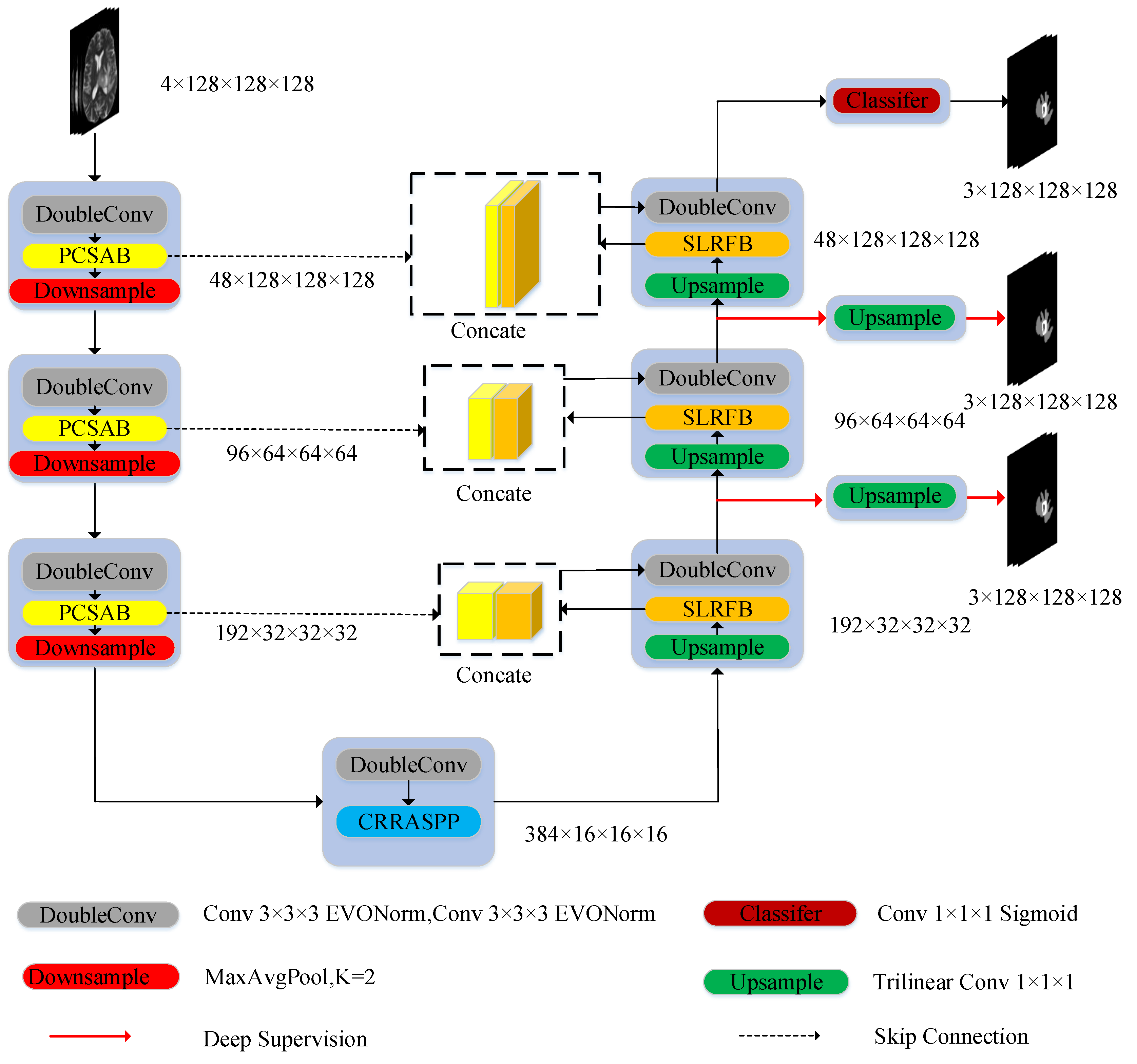
3.1. Network Architecture

To better segment brain tumor MRI images, the network adopts a U-shaped symmetric structure, as shown in Figure 1. Corresponding to the decoder on the right is the encoder on the left. On the right side of the decoder is the deep supervision module, and at the bottom of the network architecture is the bottleneck layer. The left encoder consists of three layers, each of which is referred to as an encoding block. Each encoding block is composed of three parts: two convolutions with a kernel size of 3 × 3 × 3 and a stride of 1. To reduce the impact on the batch and improve segmentation performance, an evolving normalization–activation layer (EVO Norm) [28] is placed after each convolution. Following the normalization is the PCSAB attention module for extracting fine features, in turn followed by the downsampling. The downsampling uses maximum average pooling with a kernel size of 2 to reduce the image size to half of the original. On the right side of the network is the decoder, which is also divided into three layers. Each layer contains a decoding block, which is divided into three parts. The first part is an upsampling module, which includes trilinear interpolation and convolution with a kernel size of 1 × 1 × 1 and a stride of 1 to restore the image size, doubling the size of the image. The second part is the SLRFB attention module, which follows its upsampling counterpart to enhance the receptive field. The third part consists of two convolutions with a kernel size of 3 × 3 × 3 and a stride of 1, with EVO Norm normalization following each convolution. Between the corresponding layers of the encoder and decoder, skip connections are used to transmit information. The difference from the traditional 3D U-Net in this part is that the information passed from the encoder is concatenated with the information processed by the SLRFB attention module before being passed to the DoubleConv module for processing. At the bottom of the network is the bottleneck layer, which includes two parts. First, there are two convolutions with a kernel size of 3 × 3 × 3 and a stride of 1, with EVO Norm normalization following each convolution. Second, there is the CRRASPP module to enhance the interaction between different pieces of information. At the end of the network, a convolution with a kernel size of 1 × 1 × 1 and a stride of 1 is used as the classifier to restore the image size to 128 × 128 × 128, and the number of channels is changed to three, each channel storing the obtained WT, TC, and ET results, respectively.

3.2. Parallel Channel and Spatial Attention Block (PCSAB)

In the process of brain tumor MRI image segmentation, the encoding process is an important step for obtaining features. Effective feature extraction is crucial for the final segmentation; in particular, the effective fusion of global and local features plays a significant role. However, the effective extraction of global and local features is one of the current research challenges. The PSCAB module can enhance the fusion and extraction of details and global information by using spatial and channel attention as optimization means. A diagram of the PSCAB block is shown in Figure 2. It mainly consists of three parts: the channel attention mechanism (the upper part in Figure 2), the original information retention part (the middle part), and the spatial attention mechanism (the lower part). Channel attention first uses global average pooling to obtain as much global information as possible, then maps the image with global feature information to one-dimensional features, called $F_{map}$ operation, and uses a one-dimensional convolution with a kernel size of 3 and a stride of 1 to capture the interaction information between different features, learning the complex relationships between local features. Then, the information is restored to three-dimensional information, and the channel weights are obtained through the Sigmoid activation function.

The process of obtaining global features and transforming three-dimensional data into one-dimensional data can be mathematically expressed as follows:

$$X_{map}=F_{map}\left(GlobalAvgPool\right(x\left)\right)$$

(1)

where x represents the input data, while $X_{map}$ denotes the output result of the mapping operation. $GlobalAvgPool$ denotes global average pooling and $F_{map}$ indicates the mapping operation.

The operation of integrating detailed information and restoring one-dimensional data to three-dimensional data can be defined as follows:

$$x^{’}=F_{anti-map}\left({Conv}_{1d}\right(X_{map}\left)\right)$$

(2)

where $x^{’}$denotes the output result of this operation, while $F_{anti-map}$ indicates the transformation that restores one-dimensional data back to its three-dimensional form. ${Conv}_{1d}$denotes a one-dimensional convolution with a kernel size of 3 and a stride of 1.

Channel attention can be represented as follows:

$$X_{channel}=Sigmoid\left(x^{’}\right)$$

(3)

where $x^{’}$ represents the input data, while $X_{channel}$ represents the output result of channel attention.

In the lower half of the PSCAB module lies the spatial attention mechanism. Initially, average pooling and maximum pooling are employed to retain comprehensive information and accentuate local salient features, with a particular focus on edge details. Subsequently, the feature information derived from both average and maximum pooling is concatenated. This combined feature set is then processed through a convolutional layer featuring a 3 × 3 × 3 kernel and a stride of 1, enabling the extraction of refined features. Ultimately, the resultant feature map, enhanced by spatial attention, is generated via the Sigmoid activation function. Spatial attention can be described as follows:

$$X_{spatial}={Sigmoid(Conv}_{3\times 3\times 3}\left(concate\left(maxpool\left(x\right),avgpool\left(x\right)\right)\right))$$

(4)

where x represents the input data. The $maxpool$ and $avgpool$ terms can be respectively expressed as maximum pooling and average pooling. ${Conv}_{3\times 3\times 3}$represents a convolution operation with a kernel size of 3 × 3 × 3 and a stride of 1. After the convolution, InstanceNorm normalization and LeakyReLU activation function operations are applied.

To capture features that elude spatial and channel attention mechanisms, the PSCAB module preserves the original information in its central section. This allows for the extraction of more nuanced edge and texture details, enriching the feature set. Consequently, the learned features become more holistic, as the retained original data contribute to subsequent processing steps. As a result, the feature information obtained from the PSCAB attention is as follows:

$$Y_{out}=X_{channel}\times x\times X_{spatial}$$

(5)

where $Y_{out}$ represents the feature information after processing through PSCAB. $X_{channel}$, $x$ , and $X_{spatial}$ correspond to the results after channel attention processing, the original information, and spatial attention processing, respectively.

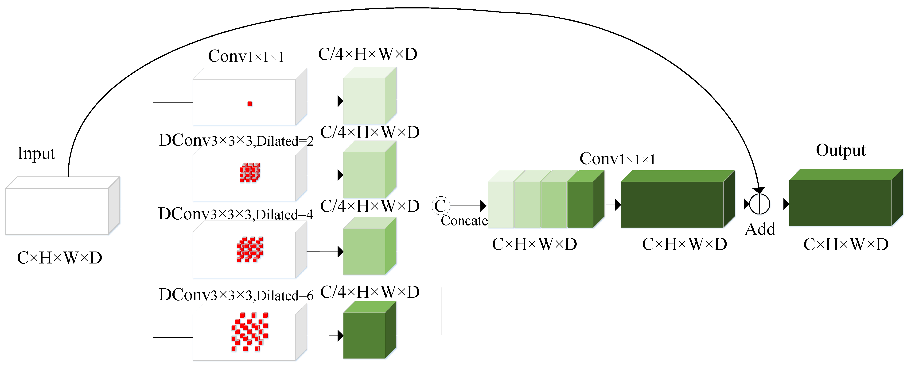
3.3. Channel Reduce Residual Atrous Spatial Pyramid Pooling Block (CRRASPP)

Situated at the terminal end of the encoder, the bottleneck layer emerges after the input image has undergone a cascade of downsampling and convolutional transformations. In this process, the spatial dimensions of the input image undergo a marked contraction, while there is a concomitant surge in the number of channels. The iterative downsampling imparts to the bottleneck layer’s feature maps an expansive receptive field, enabling them to encompass the vast majority of the input image, thereby encapsulating global contextual information. This endows the model with an enhanced capacity to comprehend the overarching structure and semantic nuances of the image, thus establishing a robust groundwork for the ensuing decoder to execute precise segmentation tasks. Functioning as a pivotal conduit between the encoder and decoder, the bottleneck layer facilitates the transfer of high-level features, meticulously extracted by the encoder, to the decoder. This transfer is instrumental in providing the decoder with crucial sustenance for its subsequent undertakings of upsampling and the intricate process of feature amalgamation. Nevertheless, considering the inherent complexity and variety of features within the bottleneck layer, adeptly capturing features across multiple scales serves to amplify their expressive capabilities. Consequently, this enrichment renders the features more aptly tailored for the ensuing processes of upsampling and segmentation, thereby elevating the overall efficacy of these tasks.

As shown in Figure 3, to capture multiscale features, in the CRRASPP module, a convolution with a kernel size of 1 × 1 × 1, a stride of 1, and dilated convolutions with a kernel size of 3 × 3 × 3, a stride of 1, and dilation rates of 2, 4, and 6 are first employed to extract multiscale features. In order to reduce the number of model parameters, the number of channels in the image is reduced to a quarter of the original following each dilated convolution. Subsequently, the four dilated convolutions with different dilation rates are concatenated and then aggregated via a convolution with a kernel size of 1 × 1 × 1 and a stride of 1. To enhance the feature representation capability, the features are abstracted and subjected to further learning in conjunction with the input data features, thereby preserving the key information. The CRRASPP block can be described as follows:

$$U_{out}=x+{Conv}_{1\times 1\times 1}\left(concate\right({{Conv}_{1\times 1\times 1},DConv}_{3\times 3\times 3}(x,{\theta }_i)\left)\right),{\theta }_i\in \{2,4,6\}$$

(6)

where $U_{out}$ represents the output features processed by the CRRASPP attention mechanism, ${Conv}_{1\times 1\times 1}$ refers to a convolution with a kernel size of 1 × 1 × 1 and a stride of 1, the concate operation indicates the concatenation operation, and ${DConv}_{3\times 3\times 3}$ describes a dilated convolution with a kernel size of 3 × 3 × 3, a stride of 1, and a dilation rate of ${\theta }_i$, where the value of the dilation rate $\theta$ is $\{2,4,6\}$.

3.4. Selective Large Receptive Field Block (SLRFB)

During the upsampling stage, to comprehensively capture multiscale image feature information, the designed SLRFB attention module employs group convolutions with different kernel sizes and varying dilation rates. To more effectively capture features, a group convolution with a kernel size of 3 × 3 × 3 is applied first, followed by a group convolution with a kernel size of 5 × 5 × 5 and a dilation rate of 2. As shown in Figure 4, to capture more valuable information after obtaining multiscale features, a channel attention mechanism identical to the upper part of the PCSAB attention is utilized to capture different weights, identify the most contributive channels, and reduce the impact of irrelevant or redundant channels. This process enables the model to focus on key features, thereby enhancing segmentation performance.

The SLRFB consists of three parts: a group convolution with a kernel size of 3 × 3 × 3, a group convolution with a kernel size of 5, and channel attention. The group convolution with a kernel size of 3 × 3 × 3 can be described as follows:

$${KGC}_3\left(x\right)=groupCon{v}_{3\times 3\times 3}\left(x,G,\theta \right)$$

(7)

where ${KGC}_3$represents the result after processing through a group convolution with a kernel size of 3 × 3 × 3. Here, x is the input feature. The $groupCon{v}_{3\times 3\times 3}$denotes the group convolution, where the parameter $G$ represents the number of groups which is equal to the number of input channels, and $\theta$ denotes the dilation rate, which is set to 1.

The group convolution with a kernel size of 5 × 5 × 5 can be described as follows:

$${KGC}_5\left(x\right)=groupCon{v}_{5\times 5\times 5}\left({KGC}_3\left(x\right),G,\theta \right)$$

(8)

where${KGC}_5$denotes the output result. The input feature is ${KGC}_3\left(x\right)$. The $groupCon{v}_{5\times 5\times 5}$ refers to the group convolution with a kernel size of 5 × 5 × 5, where the parameter $G$ represents the number of groups, equal to the number of input channels, and $\theta$ denotes the dilation rate, which is set to 2.

The channel attention mechanism can be expressed as follows:

$${CA}_{out}=CA\left(concate\right({KGC}_3\left(x\right),{KGC}_5\left(x\right)\left)\right)$$

(9)

where ${CA}_{out}$ is the output result and $CA$ denotes the channel attention operation.

The SLRFB attention mechanism is a combination of ${KGC}_3\left(x\right)$, ${KGC}_5\left(x\right)$, and ${CA}_{out}$and can be described as follows:

$$Z_{out}={CA}_{out}\times ({KGC}_3\left(x\right)+{KGC}_5\left(x\right))$$

(10)

where $Z_{out}$ represents the feature extracted following the application of the SLRFB attention mechanism.

4. Experiments and Results

4.1. Datasets and Preprocessing

To evaluate the segmentation performance on brain tumor MRI images, we selected the publicly available and freely usable BraTS (Brain Tumor Segmentation) challenge dataset, which includes BraTS2019, BraTS2020, and BraTS2021 [29,30,31]. Among the three datasets, the BraTS2019 dataset includes 335 training cases and 125 validation cases, the BraTS2020 dataset includes 369 training cases and 125 validation cases, and the BraTS2021 dataset includes 1251 training cases and 219 validation cases. All training data included images manually annotated by neuroradiologists. The validation data used for online validation contained manually annotated images that were not publicly accessible. During validation, the model was first trained on a local server. Upon completion of training, online validation was performed on the Synapse platform, where the final evaluation results were obtained. The Synapse platform is accessible via https://www.synapse.org/#platform (accessed on 14 March 2025).

The images in the BraTS dataset contain a significant amount of black background. To focus more on the analysis and processing of brain images, the black background was removed as much as possible during the preprocessing stage. In this process, the input image volume was cropped to the minimum bounding box containing nonzero voxels, and then the image size was cropped from 240 × 240 × 155 to 128 × 128 × 128 using the random cropping method, and then the input image was preprocessed by z-score normalization. To minimize the impact on segmentation performance, all intensity values were clipped to the 1st and 99th percentiles of the non-zero voxel distribution within the volume. Data augmentation was also employed in this study, including random Gaussian noise, rand smoothing, random flip, random shift, random contrast intensity adjustment, and random rotation of 90 degree.

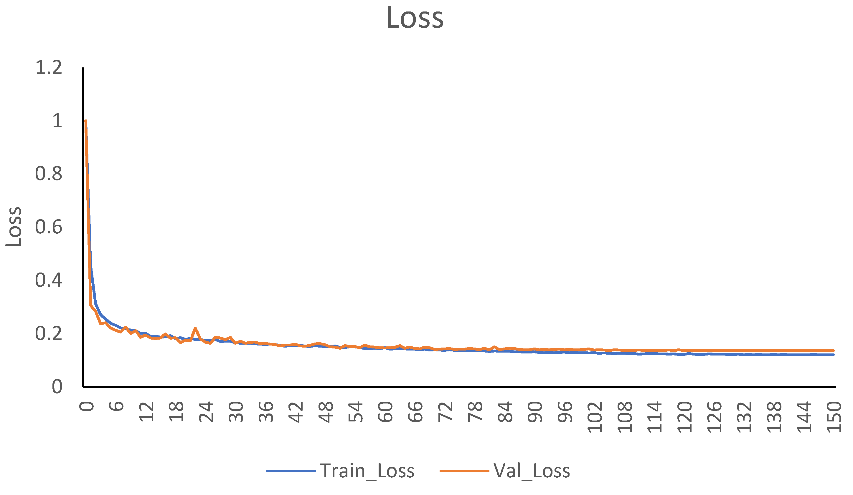
4.2. Implementation Details

MEASegNet was developed using Python 3.8.10 and PyTorch 1.11.0. The server configuration used includes an AMD EPYC 7551P processor (AMD, Santa Clara, CA, USA) and a single NVIDIA RTX A5000 graphics card (PNY, Parsippany, NJ, USA). The initial learning rate was set to 3.00 × 10⁻⁴. Due to the computational limitations of the server, the batch size was set to 1 in the experiments. As shown in

Table 1. Model parameter configuration.

Basic Configuration	Value
PyTorch version	1.11.0
Python	3.8.10
GPU	NVIDIA RTX A5000 (24 G)
Cuda	cu113
Learning rate	3.00 × 10−4
Optimizer	Ranger
Batch size	1
Loss	Jaccard loss
Epoch	150
Input size	128 × 128 × 128
Output size	128 × 128 × 128

, the Ranger [32] optimizer was used to enhance the stability of the model during training and accelerate the convergence speed, while the Jaccard loss function was used to solve the class imbalance problem during brain tumor segmentation.

4.3. Evaluation Metrics and Loss Function

To effectively evaluate the final results, the Dice Similarity Coefficient (Dice) [33] score and the Hausdorff distance (HD) [34,35] were employed in this study. The similarity between the two groups was measured by the Dice score. During image segmentation, it is used to evaluate the similarity between the predicted segmentation results and manual annotations, and is expressed as follows:

$$Dice={\displaystyle \frac{(2\times \mathrm{p}\mathrm{r}\mathrm{e}\mathrm{d}\mathrm{i}\mathrm{c}\mathrm{t}\mathrm{V}\mathrm{a}\mathrm{l}\mathrm{u}\mathrm{e})\cap (2\times \mathrm{m}\mathrm{a}\mathrm{n}\mathrm{u}\mathrm{a}\mathrm{l}\mathrm{V}\mathrm{a}\mathrm{l}\mathrm{u}\mathrm{e})}{predictValue+manualValue}}$$

(11)

where $predictValue$ represents the result predicted by the model, while $manualValue$ represents the value manually annotated by neuroradiologists.

The Hausdorff distance (HD) represents the maximum distance between the predicted and actual boundaries. A lower HD value indicates smaller errors. The HD can be mathematically expressed as follows:

$$D(P,T)=\mathrm{m}\mathrm{a}\mathrm{x}\{su{p}_{t\in T}in{f}_{p\in P}d\left(t,p\right),su{p}_{p\in P}in{f}_{t\in T}d\left(t,p\right)\}$$

(12)

where $t$ and $p$ represent the actual region boundary and the predicted segmentation region boundary, respectively. The term $d\left(·\right)$ denotes the distance between $t$ and $p$. The term$sup$ represents the supremum (least upper bound), while the $inf$ term represents the infimum (greatest lower bound).

Considering the class imbalance problem in brain tumor subregions, the Jaccard loss function was introduced. This loss function is derived from the Jaccard coefficient, also known as Intersection over Union (IoU), which measures the similarity of two sets. The Jaccard loss function can directly calculate the matching degree between the tumor region predicted by the model and the real tumor region in the image, thus playing an important role in improving the performance of brain tumor segmentation tasks. In addition, the Jaccard loss function is more robust to the class imbalance situation when the target area is small and the background area is large, alleviating the large difference between the number of foreground and background pixels, to a certain extent, and improving the segmentation effect. The Jaccard loss function is expressed as follows:

$$\mathrm{Los}{\mathrm{s}}_{\mathrm{Jaccard}}=1-{\displaystyle \frac{\mathrm{p}\mathrm{r}\mathrm{e}\mathrm{d}\mathrm{i}\mathrm{c}\mathrm{t}\mathrm{V}\mathrm{a}\mathrm{l}\mathrm{u}\mathrm{e}\cap \mathrm{m}\mathrm{a}\mathrm{n}\mathrm{u}\mathrm{a}\mathrm{l}\mathrm{V}\mathrm{a}\mathrm{l}\mathrm{u}\mathrm{e}}{predictValue\cup manualValue}}$$

(13)

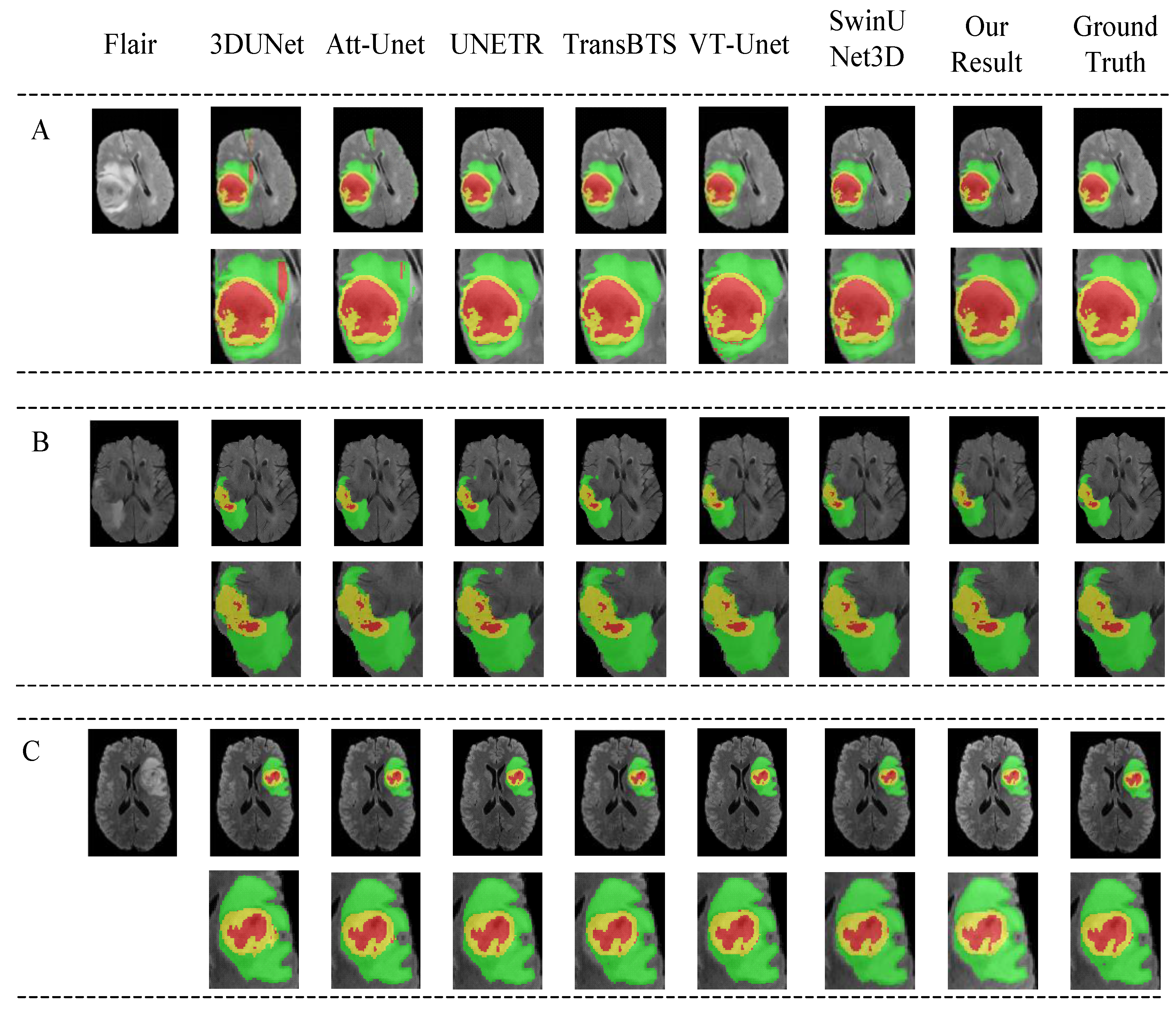
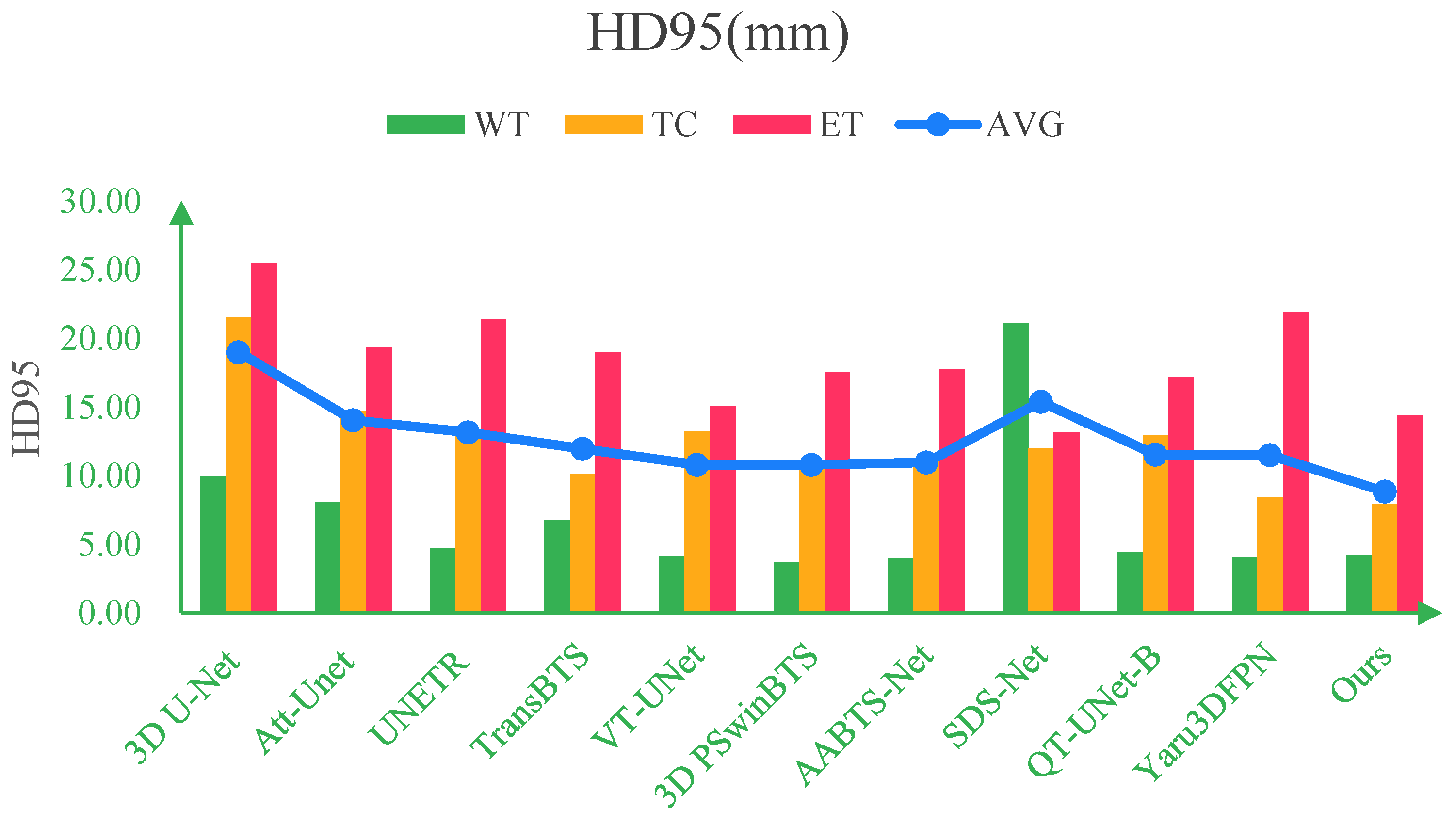
4.4. Comparison with Other Methods

To evaluate the performance of the MEASegNet model, we compared it with 11 popular models. Among them, two models were published in 2024 (Yaru3DFPN and QT-UNet-B), two in 2023 (Swin Unet3D and SDS-Net), and two in 2022 (AABTS-Net and 3D PSwinBTS); the other five are classic models (3D U-Net, Att-Unet, UNETR, TransBTS, and VT-UNet). Among these models, those combining U-Net with attention mechanisms are Att-Unet, AABTS-Net, and SDS-Net, while the Transformer-based models are UNETR, TransBTS, 3D PSwinBTS, Swin Unet3D, and QT-UNet-B. The results of MEASegNet and the 11 networks on the BraTS2021 dataset online validation are shown in

Table 2. The online validation results for the comparison of different methods in relation to BraTS2021, with the best performance highlighted in bold.

Methods	Dice (%)				HD95 (mm)
	WT	TC	ET	AVG	WT	TC	ET	AVG
3D U-Net (2016) [10]	88.02	76.17	76.20	80.13	9.97	21.57	25.48	19.00
Att-Unet (2018) [36]	89.74	81.59	79.60	83.64	8.09	14.68	19.37	14.05
UNETR (2021) [37]	90.89	83.73	80.93	85.18	4.71	13.38	21.39	13.16
TransBTS (2021) [38]	90.45	83.49	81.17	85.03	6.77	10.14	18.94	11.95
VT-UNet (2022) [39]	91.66	84.41	80.75	85.60	4.11	13.20	15.08	10.80
3D PSwinBTS (2022) [40]	92.64	86.72	82.62	87.32	3.73	11.08	17.53	10.78
AABTS-Net (2022) [41]	92.20	86.10	83.00	87.10	4.00	11.18	17.73	10.97
SDS-Net (2023) [42]	91.80	86.80	82.50	87.00	21.07	11.99	13.13	15.40
Swin Unet3D (2023) [43]	90.50	86.60	83.40	86.83	-	-	-	-
QT-UNet-B (2024) [44]	91.24	83.20	79.99	84.81	4.44	12.95	17.19	11.53
Yaru3DFPN (2024) [45]	92.02	86.27	80.90	86.40	4.09	8.43	21.91	11.48
Our(MEASegNet)	92.50	87.49	84.16	88.05	4.18	7.96	14.40	8.85

and Figure 5.

The online validation results of the MEASegNet model for WT, TC, ET, and average Dice were 92.5%, 87.49%, 84.16%, and 88.05%, respectively. As shown in Figure 6, the HD95 results were 4.18, 7.96, 14.40, and 8.85, respectively. The 3D PSwinBTS model outperformed MEASegNet in relation to WT due to its advantages in modeling global or long-range contextual interactions and spatial dependencies. However, MEASegNet achieved higher Dice values with respect to TC and ET compared to 3D PSwinBTS thanks to the attention mechanisms incorporated at various stages of feature acquisition and processing. Additionally, MEASegNet exhibited slightly higher Dice values than the other networks listed in Table 2. From the HD95 perspective, 3D PSwinBTS and SDS-Net performed slightly better than MEASegNet, but the differences were not significant. Among the compared networks, MEASegNet had relatively lower HD95 values with respect to TC and ET, also indicating that the segmentation results were within an acceptable range.

In order to further verify the segmentation ability of MEASegNet, the offline experimental results of six popular models, i.e., 3D U-Net, Att-UNet, UNETR, TransBTS, VT-UNet, and Swin Unet3D, were obtained through model training in the same experimental environment.

Table 3. The offline validation results for the comparison of different methods in relation to BraTS2021, with the best performance highlighted in bold.

Methods	Dice (%)				HD95 (mm)
	WT	TC	ET	AVG	WT	TC	ET	AVG
3D U-Net [10]	91.29	89.13	85.78	88.73	7.50	5.47	3.82	5.59
Att-Unet [36]	91.43	89.51	85.71	88.88	7.30	5.39	3.81	5.50
UNETR [37]	91.53	88.57	85.27	88.46	7.42	5.98	3.74	5.71
TransBTS [38]	90.61	88.78	84.29	87.89	7.64	5.56	3.90	5.70
VT-UNet [39]	92.39	90.12	86.07	89.53	7.14	5.17	3.97	5.42
Swin Unet3D [43]	92.85	90.69	86.26	89.93	7.17	4.94	3.83	5.31
Our (MEASegNet)	93.29	93.16	88.19	91.55	6.87	4.57	3.59	5.01

shows the offline experimental results of MEASegNet and six popular models. As it can be seen in Table 3, MEASegNet achieved a outperformance in terms of the Dice score and HD95.

In order to verify that the difference in Dice scores of MEASegNet was not generated by random variation but by the actual model, performance was improved. We conducted paired t-test experiments to verify that the improvement in MEASegNet was statistically significant. The offline results of the above six popular models and the experimental results are shown in

Table 4. Ratio (in %) of the improvement in the performance of MEASegNet compared to different methods. Bold numbers indicate statistical significance (p < 0.05).

Methods	WT		TC		ET
	%Subjects	p	%Subjects	p	%Subjects	p
MEASegNet (ours) vs. 3D U-Net	78.09	7.427 × 10−15	84.86	2.499 × 10−10	79.68	0.0007
MEASegNet (ours) vs. Att-Unet	77.69	5.505 × 10−8	84.06	1.087 × 10−8	79.68	0.0032
MEASegNet (ours) vs. UNETR	77.29	2.481 × 10−7	86.45	1.837 × 10−9	80.48	0.0022
MEASegNet (ours) vs. TransBTS	82.87	1.046 × 10−7	85.66	1.197 × 10−8	82.87	5.048 × 10−6
MEASegNet (ours) vs. VT-UNet	73.71	0.0052	82.87	2.370 × 10−7	78.88	0.0048
MEASegNet (ours) vs. Swin Unet3D	71.71	0.0047	81.27	5.619 × 10−6	78.49	0.0182

.

As it can be seen in Table 4, the p-values of the Dice scores for MEASegNet and the other models were all less than 0.05, indicating that the Dice values of different models in the table are significantly different.

In order to test the generalization of the proposed model, MEASegNet was trained and evaluated using two datasets, i.e., BraTS2019 and BraTS2020, under the same experimental conditions and training parameters. Since the online evaluation platform of the BraTS2019 and BraTS2020 datasets is no longer in use, the training set of the two datasets were divided into the model training set and the model validation set according to the ratio of 4:1, and the validation set results of the model were referred to as the offline results. The segmentation effect of MEASegNet on BraTS2020 and BraTS2019 was evaluated using the model validation set.

MEASegNet was compared with five excellent networks, namely AMPNet, 3D U-Net, DMFNet, CANet, and AE AU-Net, in relation to the BraTS2019 dataset. Among them, 3D U-Net is a classic network, while the other four network structures are inspired to the encoder–decoder structure.

Table 5. The offline validation results for the comparison of different methods in relation to BraTS2019, with the best performance highlighted in bold.

Methods	Dice (%)				HD95 (mm)
	WT	TC	ET	AVG	WT	TC	ET	AVG
AMPNet [46]	90.29	79.32	75.57	81.73	4.49	8.19	4.77	5.82
3D U-Net [10]	88.40	79.60	77.60	81.87	9.11	8.68	4.48	7.42
DMFNet [47]	90.00	81.50	77.60	83.03	4.64	6.22	2.99	4.62
CA Net [48]	88.50	85.10	75.90	83.17	7.09	8.41	4.81	6.77
AE AU-Net [49]	90.20	81.50	77.30	83.00	6.15	7.54	4.65	6.11
Our (MEASegNet)	90.24	88.80	80.36	86.47	7.85	6.10	4.08	6.01

shows the comparison between MEASegNet and the other excellent networks.

As it can be seen from Table 5, the Dice scores of MEASegNet with respect to WT, TC, and ET of the BraTS2019 model validation set were 90.24%, 88.80%, and 80.36%, and the HD95 were 7.85, 6.10, and 4.08. Among them, the Dice score of AMPNet in the WT region was slightly higher than that of MEASegNet, because its model prediction part takes the minimum value at different resolutions and aggregates the information of multiscale prediction. However, MEASegNet achieved better Dice scores than AMPNet with respect to TC and ET regions. MEASegNet showed better results in terms of Dice scores compared to the remaining models in the table. Concerning HD95, AMPNet and DMFNet performed slightly better in terms of WT and ET, while MEASegNet showed a slight advantage with respect to TC.

MEASegNet was also compared with four excellent networks, i.e., U-Net++, Point-UNet, TransBTS, and RFNet, with respect to the BraTS2020 dataset. Among them, Point-UNet combines U-Net with Point cloud technology, and TransBTS combines Transformer and U-Net structures. The MEASegNet results using the BraTS2020 dataset are shown in

Table 6. The offline validation results for the comparison of different methods in relation to BraTS2020, with the best performance highlighted in bold.

Methods	Dice (%)
	WT	TC	ET	AVG
U-Net++ [50]	89.77	85.57	79.83	85.06
Point-UNet [51]	89.67	82.97	76.43	83.02
TransBTS [38]	90.09	81.73	78.73	83.52
RFNet [52]	91.11	85.21	78.00	84.77
Our (MEASegNet)	91.66	86.97	79.09	85.91

, where they are compared to the results of the other networks.

As it can be seen from Table 6, the Dice scores of MEASegNet with respect to WT, TC, and ET of the BraTS2020 dataset were 91.66%, 86.97%, and 79.09%. MEASegNet showed the best performance in terms of the Dice score compared to the other models in the table. Among them, the Dice score of U-Net++ was 0.74% higher than that of MEASegNet in the ET region, because it introduces dense connections in the skip structure to fuse features of multiple scales at different levels. However, MEASegNet achieved better Dice scores than U-Net++ with respect to WT and TC regions.

Given the significant impact of small targets and data class imbalance on segmentation outcomes in brain tumor MRI images, the Jaccard loss function was employed in MEASegNet. This choice was driven by its superior ability to enhance segmentation accuracy and its robust performance in handling small targets and imbalanced datasets. As illustrated in Figure 7, the network stabilized by epoch 150, yielding a smooth curve that attests to the model’s rapid convergence and efficient inference capabilities.

To verify the actual segmentation outcomes, three FLAIR image cases were randomly chosen from the BraTS2021 dataset for segmentation evaluation. The models used for comparison, from left to right, included 3D U-Net, Att-Unet, UNETR, TransBTS, VT-Unet, Swin UNet3D, and MEASegNet (ours), with the manually annotated ground-truth segmentation on the right. As depicted in Figure 8, the segmentation results generated by MEASegNet (ours) more closely resembled the ground-truth images than those produced by other segmentation methods, thereby highlighting the practical potential of MEASegNet.

5. Ablation Experiments

5.1. Ablation Study of Each Module in MEASegNet

In the MEASegNet network, we incorporated three distinct attention modules: the PCSAB within the encoder, the CRRASPP in the bottleneck layer, and the SLRFB in the decoder. An ablation experiment entails “removing” or “eliminating” certain components of the model to assess how their removal affects the overall effect. To systematically assess their individual contributions, we performed ablation experiments (Expt) on these modules.

As illustrated in

Table 7. Results of the ablation studies of each module in MEASegNet, with the best performance highlighted in bold.

NO	Expt	Dice (%)				HD95 (mm)
		WT	TC	ET	AVG	WT	TC	ET	AVG
A	Base	90.83	85.93	82.54	86.43	6.00	10.47	16.97	11.15
B	Base+SLRFB	92.17	86.61	82.75	87.18	5.02	8.37	19.72	11.04
C	Base+CRRASPP	91.67	86.76	83.48	87.30	4.74	10.25	13.31	9.43
D	Base+PCSAB	92.07	86.46	82.70	87.08	4.67	10.41	18.56	11.21
E	Base+SLRFB+CRRASPP	92.28	86.58	83.72	87.53	4.39	10.14	13.20	9.24
F	Base+SLRFB+PCSAB	92.21	87.11	83.76	87.69	5.00	9.81	17.91	10.91
G	Base+PCSAB+CRRASPP	92.22	87.05	82.94	87.40	4.49	8.85	18.75	10.70
H	Base+PCSAB+CRRASPP+SLRFB	92.50	87.49	84.16	88.05	4.18	7.96	14.40	8.85

and Figure 9 and Figure 10, the average (AVG) Dice score improved by 0.75% (Experiment B), 0.87% (Experiment C), and 0.65% (Experiment D) when SLRFB, CRRASPP, and PCSAB were individually integrated into the baseline network, respectively. Except for Experiment D, the average HD95 values were also optimized. To assess the synergistic effects of the developed attention mechanisms, we performed experiments with various combinations of SLRFB, CRRASPP, and PCSAB. The results demonstrate that the pairwise combinations of these attention modules consistently enhanced both the average Dice score and HD95 values compared to the baseline network. When all three attention mechanisms were applied concurrently, the optimal performance was achieved. Specifically, the Dice values for WT, TC, ET, and the average reached 92.50%, 87.49%, 84.16%, and 88.05%, respectively, while the HD95 values for WT, TC, ET, and the average were 4.18, 7.96, 14.40, and 8.85, respectively.

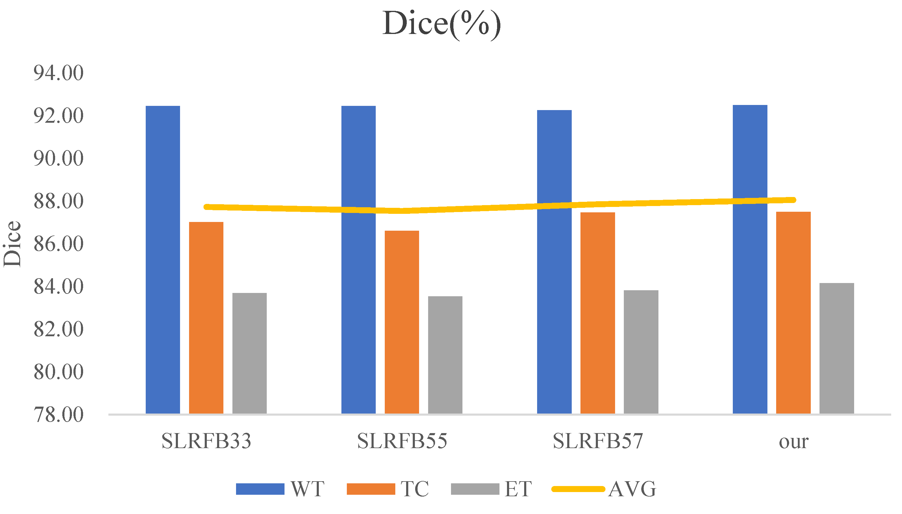
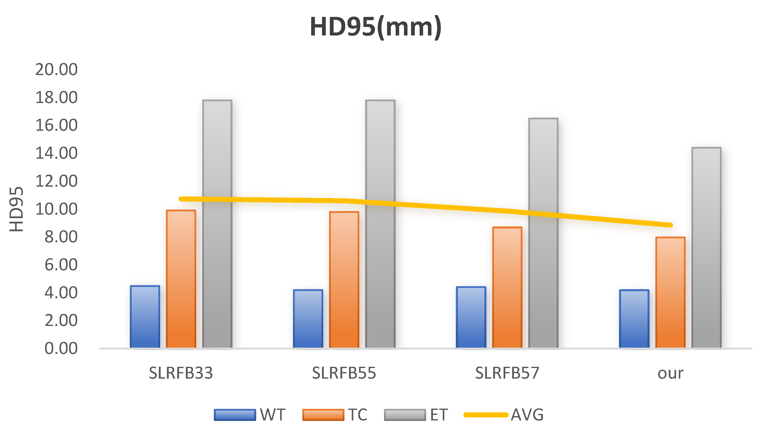
5.2. The Studies of Different Convolutional Kernels in SLRFB in the Context of Multiscale Feature Extraction

The efficacy of the SLRFB attention module compared to the baseline network was established, with the results reported in Table 7. However, the capacity to capture multiscale features can differ significantly depending on the combination of the convolutional kernels employed. To explore how different convolutional kernels influence the MEASegNet network, this study conducted three sets of experiments. These experiments tested sequential kernel sizes of 3 × 3 × 3 followed by 3 × 3 × 3 (SLRFB33), 3 × 3 × 3 followed by 5 × 5 × 5 (SLRFB35), 5 × 5 × 5 followed by 5 × 5 × 5 (SLRFB55), and 5 × 5 × 5 followed by 7 × 7 × 7 (SLRFB57).

As indicated in

Table 8. The results of ablation experiments for different convolutional kernels in SLRFB, with the best performance highlighted in bold.

Methods	Dice (%)				HD95 (mm)
	WT	TC	ET	AVG	WT	TC	ET	AVG
SLRFB33	92.46	87.01	83.69	87.72	4.48	9.9	17.80	10.73
SLRFB55	92.46	86.61	83.53	87.53	4.19	9.79	17.80	10.59
SLRFB57	92.26	87.47	83.81	87.85	4.4	8.68	16.49	9.86
SLRFB35 (our)	92.50	87.49	84.16	88.05	4.18	7.96	14.40	8.85

, the SLRFB35 experiment demonstrated superior performance, achieving Dice values of 92.50% for WT, 87.49% for TC, 84.16% for ET, and an average of 88.05%. The corresponding HD95 values were 4.18 for WT, 7.96 for TC, 14.40 for ET, and an average of 8.85. Figure 11 and Figure 12 further reveal that larger convolutional kernels did not always result in improved performance. In fact, it is the judicious selection of kernel sizes that leads to optimal outcomes, particularly within the decoder.

5.3. The Studies of ASPP, CRRASPP, and Deep Supervision

Table 7 has already demonstrated the effectiveness of CRRASPP in the bottleneck layer. However, the ASPP [53] module is also capable of capturing multiscale feature information. To conclusively prove that CRRASPP outperforms the ASPP module, a comparative experiment was conducted between the two. Additionally, deep supervision has the ability to mask irrelevant noise. To further validate the necessity of deep supervision, experiments assessing its effectiveness were also performed.

Table 9. The results of the experimental comparison between ASPP and CRRASPP.

Methods	Dice (%)				HD95 (mm)
	WT	TC	ET	AVG	WT	TC	ET	AVG
ASPP	92.29	86.28	80.71	86.43	4.52	10.24	18.43	11.06
CRRASPP (our)	92.50	87.49	84.16	88.05	4.18	7.96	14.40	8.85

demonstrates that the CRRASPP module significantly outperformed the ASPP module, particularly in the context of segmenting multiscale targets. This superiority is primarily attributed to CRRASPP’s ability to capture both global semantic information and local details more effectively through adaptive dilation rates. Moreover, the integration of 1 × 1 × 1 convolutions with a stride of 1 in CRRASPP further enhances its capacity to capture long-range contextual information.

Table 10. The results of ablation studies on deep supervision.

Methods	Dice (%)				HD95 (mm)
	WT	TC	ET	AVG	WT	TC	ET	AVG
Without deep supervision	91.63	85.03	82.43	86.36	5.64	11.36	17.37	11.46
With deep supervision (our)	92.50	87.49	84.16	88.05	4.18	7.96	14.40	8.85

demonstrates that incorporating deep supervision into the MEASegNet network led to a notable enhancement in performance. By integrating deep supervision across multiple layers, the model was able to capture more nuanced and comprehensive feature representations. This, in turn, bolstered its generalization ability when using unseen data while mitigating the influence of irrelevant noise.

5.4. The Studies of Parameters and Floating-Point Operations in MEASegNet

The influence of the attention mechanism of MEASegNet on the number of parameters and FLOPs (floating-point operations) was investigated, and the experimental results are shown in

Table 11. The results of parameters and FLOPs in MEASegNet, with the best performance highlighted in bold.

NO	Expt	Dice (%)				FLOPs (G)	Parameter (M)
		WT	TC	ET	AVG
A	Base	90.83	85.93	82.54	86.43	1056.983	14.537
B	Base+PCSAB+CRRASPP+SLRFB	92.50	87.49	84.16	88.05	1090.586	17.856

.

As it can be seen from Table 11, compared to the base network, MEASegNet increased the number of FLOPs by 33.603 G and the number of parameters by 3.319 M, although it improved the average Dice score by 1.62%. Although the increased number of FLOPs and parameters improved the dice score, the increase was small compared to their total amount, and this has implications for the study of more accurate brain tumor segmentation networks.

6. Limitations and Future Perspectives

MEASegNet achieved a certain improvement in terms of the Dice score and HD95 distance when using the three datasets BraTS2019, BraTS2020, and BraTS2021. However, there are still some challenges in the practical application of the BraTS dataset, which is manually annotated. The BraTS annotation is a widely accepted benchmark; however, differences in ratings between neuroradiologists may introduce label noise. As for how to deal with wrong annotations or inconsistencies, we introduce preprocessing methods such as Z-score normalization, clipping to the minimum bounding box containing non-zero voxels, and intensity values to the 1st and 99th percentiles of voxel distribution to solve the problem of outliers, to some extent. In addition, the motion artifact phenomenon of brain tumor images, caused by the patient’s own motion and uneven magnetic fields of hardware devices, is not dealt with in the data preprocessing process of MEASegNet, but it is an important factor affecting brain tumor segmentation and recognition. We implemented data augmentation techniques such as affine transformation to simulate motion artifacts. The Dice scores for WT, TC, and ET were 91.37%, 86.06%, and 80.06%, respectively, and the HD95 values were 5.99, 9.04, and 20.50, respectively. The performance worsened, and affine transformation had a certain impact on the final effect. Our subsequent studies will focus on the motion artifacts and on enhancing the generalization of the model, thus improving the ability of the model to be used in clinical applications.

7. Conclusions

This paper introduces MEASegNet, a U-shaped network tailored for brain tumor MRI segmentation. MEASegNet integrates three novel attention modules: PCSAB, CRRASPP, and SLRFB. SLRFB , positioned in the decoder, deeply integrates global and local features to enhance feature extraction robustness. CRRASPP, located in the bottleneck layer, captures and effectively fuses multiscale information, thereby strengthening feature interactions. PCSAB further refines these features, improving segmentation performance on the basis of enhanced multiscale information. The effectiveness of these attention modules was empirically validated. Compared with 11 state-of-the-art networks, including 3D U-Net, U-Net variants with attention mechanisms, and Transformer-based models, MEASegNet achieved superior Dice scores for WT (92.50%), TC (87.49%), ET (84.16%), and the average (88.05%). Additionally, ablation studies on the combination of PCSAB, CRRASPP, and SLRFB demonstrated that integrating diverse attention mechanisms at different stages of the 3D U-Net architecture significantly boosts its performance. These results highlight the fact that designing specialized attention modules for distinct regions and integrating them effectively can markedly enhance the brain tumor MRI segmentation capabilities of 3D U-Net. In the network’s bottleneck layer, capturing multiscale features is advantageous, but it is not always the case that more scales lead to better performance. Effective fusion of multiscale features and enhanced interactions between feature information are also crucial in this layer. Moreover, our medical case visualization studies confirm the feasibility of using MEASegNet for segmenting brain tumor MRI images. We believe that our method provides a robust theoretical foundation for future research and offers valuable insights for developing treatment plans for brain tumors.

References

1. De Simone, M.; Iaconetta, G.; Palermo, G.; Fiorindi, A.; Schaller, K.; De Maria, L. Clustering functional magnetic resonance imaging time series in glioblastoma characterization: A review of the evolution, applications, and potentials. Brain Sci. 2024, 14, 296. [Google Scholar] [CrossRef] [PubMed]
2. Owonikoko, T.K.; Arbiser, J.; Zelnak, A.; Shu, H.-K.G.; Shim, H.; Robin, A.M.; Kalkanis, S.N.; Whitsett, T.G.; Salhia, B.; Tran, N.L. Current approaches to the treatment of metastatic brain tumours. Nat. Rev. Clin. Oncol. 2014, 11, 203–222. Available online: https://www.nature.com/articles/nrclinonc.2014.25 (accessed on 4 September 2024).
3. De Simone, M.; Conti, V.; Palermo, G.; De Maria, L.; Iaconetta, G. Advancements in glioma care: Focus on emerging neurosurgical techniques. Biomedicines 2023, 12, 8. [Google Scholar] [CrossRef] [PubMed]
4. Vadhavekar, N.H.; Sabzvari, T.; Laguardia, S.; Sheik, T.; Prakash, V.; Gupta, A.; Umesh, I.D.; Singla, A.; Koradia, I.; Patiño, B.B.R. Advancements in Imaging and Neurosurgical Techniques for Brain Tumor Resection: A Comprehensive Review. Cureus 2024, 16, e72745. Available online: https://pmc.ncbi.nlm.nih.gov/articles/PMC11607568/ (accessed on 7 November 2024).
5. Pulumati, A.; Pulumati, A.; Dwarakanath, B.S.; Verma, A.; Papineni, R.V. Technological advancements in cancer diagnostics: Improvements and limitations. Cancer Rep. 2023, 6, e1764. [Google Scholar]
6. Bauer, S.; Wiest, R.; Nolte, L.-P.; Reyes, M. A survey of MRI-based medical image analysis for brain tumor studies. Phys. Med. Biol. 2013, 58, R97. [Google Scholar] [CrossRef]
7. Yang, M.; Timmerman, R. Stereotactic ablative radiotherapy uncertainties: Delineation, setup and motion. Semin. Radiat. Oncol. 2018, 28, 207–217. Available online: https://www.sciencedirect.com/science/article/abs/pii/S1053429618300183 (accessed on 10 September 2024). [CrossRef]
8. Eskandar, K. Artificial Intelligence in Healthcare: Explore the Applications of AI in Various Medical Domains, Such as Medical Imaging, Diagnosis, Drug Discovery, and Patient Care. 2023. Available online: https://seriesscience.com/wp-content/uploads/2023/12/AIHealth.pdf (accessed on 14 September 2024).
9. Imtiaz, T.; Rifat, S.; Fattah, S.A.; Wahid, K.A. Automated brain tumor segmentation based on multi-planar superpixel level features extracted from 3D MR images. IEEE Access 2019, 8, 25335–25349. Available online: https://ieeexplore.ieee.org/abstract/document/8939438 (accessed on 16 September 2024).
10. Çiçek, Ö.; Abdulkadir, A.; Lienkamp, S.S.; Brox, T.; Ronneberger, O. 3D U-Net: Learning dense volumetric segmentation from sparse annotation. In Proceedings of the Medical Image Computing and Computer-Assisted Intervention–MICCAI 2016: 19th International Conference, Athens, Greece, 17–21 October 2016; Proceedings, Part II 19. pp. 424–432. Available online: https://link.springer.com/chapter/10.1007/978-3-319-46723-8_49 (accessed on 20 September 2024).
11. LeCun, Y.; Bottou, L.; Bengio, Y.; Haffner, P. Gradient-based learning applied to document recognition. Proc. IEEE 1998, 86, 2278–2324. Available online: https://ieeexplore.ieee.org/abstract/document/726791 (accessed on 25 September 2024).
12. Long, J.; Shelhamer, E.; Darrell, T. Fully convolutional networks for semantic segmentation. In Proceedings of the IEEE Conference on Computer Vision and Pattern Recognition, Boston, MA, USA, 7–12 June 2015; pp. 3431–3440. Available online: https://openaccess.thecvf.com/content_cvpr_2015/html/Long_Fully_Convolutional_Networks_2015_CVPR_paper.html (accessed on 29 September 2024).
13. Lu, H.; She, Y.; Tie, J.; Xu, S. Half-UNet: A simplified U-Net architecture for medical image segmentation. Front. Neuroinformatics 2022, 16, 911679. Available online: https://www.frontiersin.org/journals/neuroinformatics/articles/10.3389/fninf.2022.911679/full (accessed on 4 October 2024). [CrossRef]
14. Huang, K.-W.; Yang, Y.-R.; Huang, Z.-H.; Liu, Y.-Y.; Lee, S.-H. Retinal vascular image segmentation using improved UNet based on residual module. Bioengineering 2023, 10, 722. Available online: https://www.mdpi.com/2306-5354/10/6/722 (accessed on 6 October 2024). [CrossRef] [PubMed]
15. Verma, A.; Yadav, A.K. Residual learning for brain tumor segmentation: Dual residual blocks approach. Neural Comput. Appl. 2024, 36, 22905–22921. Available online: https://link.springer.com/article/10.1007/s00521-024-10380-2 (accessed on 12 October 2024). [CrossRef]
16. Kaur, A.; Singh, Y.; Chinagundi, B. ResUNet++: A comprehensive improved UNet++ framework for volumetric semantic segmentation of brain tumor MR images. Evol. Syst. 2024, 15, 1567–1585. Available online: https://link.springer.com/article/10.1007/s12530-024-09579-4 (accessed on 19 October 2024).
17. Rehman, M.U.; Ryu, J.; Nizami, I.F.; Chong, K.T. Medicine. RAAGR2-Net: A brain tumor segmentation network using parallel processing of multiple spatial frames. Comput. Biol. Med. 2023, 152, 106426. Available online: https://www.sciencedirect.com/science/article/abs/pii/S0010482522011349 (accessed on 25 October 2024). [CrossRef]
18. Chang, Y.; Zheng, Z.; Sun, Y.; Zhao, M.; Lu, Y.; Zhang, Y. Control. DPAFNet: A residual dual-path attention-fusion convolutional neural network for multimodal brain tumor segmentation. Biomed. Signal Process. Control 2023, 79, 104037. Available online: https://www.sciencedirect.com/science/article/abs/pii/S1746809422005146 (accessed on 4 November 2024).
19. Cao, Y.; Zhou, W.; Zang, M.; An, D.; Feng, Y.; Yu, B. Control. MBANet: A 3D convolutional neural network with multi-branch attention for brain tumor segmentation from MRI images. Biomed. Signal Process. Control 2023, 80, 104296. Available online: https://www.sciencedirect.com/science/article/abs/pii/S1746809422007509 (accessed on 7 November 2024). [CrossRef]
20. Liu, Z.; Cheng, Y.; Tan, T.; Shinichi, T. MimicNet: Mimicking manual delineation of human expert for brain tumor segmentation from multimodal MRIs. Appl. Soft Comput. 2023, 143, 110394. Available online: https://www.sciencedirect.com/science/article/abs/pii/S156849462300412X (accessed on 14 November 2024).
21. Jiao, C.; Yang, T.; Yan, Y.; Yang, A. RFTNet: Region–Attention Fusion Network Combined with Dual-Branch Vision Transformer for Multimodal Brain Tumor Image Segmentation. Electronics 2023, 13, 77. Available online: https://www.mdpi.com/2079-9292/13/1/77 (accessed on 17 November 2024). [CrossRef]
22. Jia, Z.; Zhu, H.; Zhu, J.; Ma, P. Two-branch network for brain tumor segmentation using attention mechanism and super-resolution reconstruction. Comput. Biol. Med. 2023, 157, 106751. Available online: https://www.sciencedirect.com/science/article/abs/pii/S0010482523002160 (accessed on 20 November 2024). [CrossRef]
23. Li, H.; Zhai, D.-H.; Xia, Y. ERDUnet: An Efficient Residual Double-coding Unet for Medical Image Segmentation. IEEE Trans. Circuits Syst. Video Technol. 2023, 34, 2083–2096. Available online: https://ieeexplore.ieee.org/abstract/document/10198487 (accessed on 22 November 2024).
24. Liu, Y.; Yao, S.; Wang, X.; Chen, J.; Li, X. MD-UNet: A medical image segmentation network based on mixed depthwise convolution. Med. Biol. Eng. Comput. 2024, 62, 1201–1212. Available online: https://link.springer.com/article/10.1007/s11517-023-03005-8 (accessed on 24 November 2024).
25. Feng, Y.; Cao, Y.; An, D.; Liu, P.; Liao, X.; Yu, B. DAUnet: A U-shaped network combining deep supervision and attention for brain tumor segmentation. Knowl. Based Syst. 2024, 285, 111348. Available online: https://www.sciencedirect.com/science/article/abs/pii/S0950705123010961 (accessed on 26 November 2024).
26. Wang, Z.; Zou, Y.; Chen, H.; Liu, P.X.; Chen, J. Multi-scale features and attention guided for brain tumor segmentation. J. Vis. Commun. Image Represent. 2024, 100, 104141. Available online: https://www.sciencedirect.com/science/article/abs/pii/S1047320324000968 (accessed on 28 November 2024).
27. Li, Y.; Kang, J. TDPC-Net: Multi-scale lightweight and efficient 3D segmentation network with a 3D attention mechanism for brain tumor segmentation. Biomed. Signal Process. Control 2025, 99, 106911. Available online: https://www.sciencedirect.com/science/article/abs/pii/S1746809424009698 (accessed on 28 January 2025). [CrossRef]
28. Liu, H.; Brock, A.; Simonyan, K.; Le, Q. Evolving normalization-activation layers. Adv. Neural Inf. Process. Syst. 2020, 33, 13539–13550. Available online: https://proceedings.neurips.cc/paper/2020/hash/9d4c03631b8b0c85ae08bf05eda37d0f-Abstract.html (accessed on 31 November 2024).
29. Bakas, S.; Akbari, H.; Sotiras, A.; Bilello, M.; Rozycki, M.; Kirby, J.S.; Freymann, J.B.; Farahani, K.; Davatzikos, C. Advancing the cancer genome atlas glioma MRI collections with expert segmentation labels and radiomic features. Sci. Data 2017, 4, 170117. Available online: https://www.nature.com/articles/sdata2017117 (accessed on 3 December 2024). [CrossRef]
30. Baid, U.; Ghodasara, S.; Mohan, S.; Bilello, M.; Calabrese, E.; Colak, E.; Farahani, K.; Kalpathy-Cramer, J.; Kitamura, F.C.; Pati, S. The rsna-asnr-miccai brats 2021 benchmark on brain tumor segmentation and radiogenomic classification. arXiv 2021, arXiv:2107.02314. [Google Scholar]
31. Menze, B.H.; Jakab, A.; Bauer, S.; Kalpathy-Cramer, J.; Farahani, K.; Kirby, J.; Burren, Y.; Porz, N.; Slotboom, J.; Wiest, R. The multimodal brain tumor image segmentation benchmark (BRATS). IEEE Trans. Med. Imaging 2014, 34, 1993–2024. Available online: https://ieeexplore.ieee.org/abstract/document/6975210 (accessed on 3 December 2024).
32. Liu, L.; Jiang, H.; He, P.; Chen, W.; Liu, X.; Gao, J.; Han, J. On the variance of the adaptive learning rate and beyond. arXiv 2019, arXiv:1908.03265. [Google Scholar]
33. Dice, L.R. Measures of the amount of ecologic association between species. Ecology 1945, 26, 297–302. Available online: https://www.jstor.org/stable/1932409 (accessed on 6 December 2024).
34. Kim, I.-S.; McLean, W. Computing the Hausdorff distance between two sets of parametric curves. Commun. Korean Math. Soc. 2013, 28, 833–850. Available online: https://koreascience.kr/article/JAKO201334064306689.page (accessed on 6 December 2024). [CrossRef]
35. Aydin, O.U.; Taha, A.A.; Hilbert, A.; Khalil, A.A.; Galinovic, I.; Fiebach, J.B.; Frey, D.; Madai, V.I. On the usage of average Hausdorff distance for segmentation performance assessment: Hidden error when used for ranking. Eur. Radiol. Exp. 2021, 5, 4. Available online: https://link.springer.com/article/10.1186/s41747-020-00200-2 (accessed on 6 December 2024). [PubMed]
36. Oktay, O.; Schlemper, J.; Folgoc, L.L.; Lee, M.; Heinrich, M.; Misawa, K.; Mori, K.; McDonagh, S.; Hammerla, N.Y.; Kainz, B.J.a.p.a. Attention u-net: Learning where to look for the pancreas. arXiv 2018, arXiv:1804.03999. [Google Scholar]
37. Hatamizadeh, A.; Tang, Y.; Nath, V.; Yang, D.; Myronenko, A.; Landman, B.; Roth, H.R.; Xu, D. Unetr: Transformers for 3d medical image segmentation. In Proceedings of the IEEE/CVF Winter Conference on Applications of Computer Vision, Waikoloa, HI, USA, 3–8 January 2022; pp. 574–584. Available online: https://openaccess.thecvf.com/content/WACV2022/html/Hatamizadeh_UNETR_Transformers_for_3D_Medical_Image_Segmentation_WACV_2022_paper.html (accessed on 8 December 2024).
38. Wenxuan, W.; Chen, C.; Meng, D.; Hong, Y.; Sen, Z.; Jiangyun, L. Transbts: Multimodal brain tumor segmentation using transformer. In Proceedings of the International Conference on Medical Image Computing and Computer-Assisted Intervention, Springer, Strasbourg, France, 27 September–1 October 2021; pp. 109–119. Available online: https://arxiv.org/abs/2103.04430 (accessed on 10 December 2024).
39. Peiris, H.; Hayat, M.; Chen, Z.; Egan, G.; Harandi, M. A robust volumetric transformer for accurate 3D tumor segmentation. In Proceedings of the International Conference on Medical Image Computing and Computer-Assisted Intervention, Singapore, 18–22 September 2022; pp. 162–172. Available online: https://springer.longhoe.net/chapter/10.1007/978-3-031-16443-9_16 (accessed on 11 December 2024).
40. Liang, J.; Yang, C.; Zeng, L. 3D PSwinBTS: An efficient transformer-based Unet using 3D parallel shifted windows for brain tumor segmentation. Digit. Signal Process. 2022, 131, 103784. Available online: https://www.sciencedirect.com/science/article/abs/pii/S1051200422004018 (accessed on 14 December 2024).
41. Tian, W.; Li, D.; Lv, M.; Huang, P. Axial attention convolutional neural network for brain tumor segmentation with multi-modality MRI scans. Brain Sci. 2022, 13, 12. Available online: https://www.mdpi.com/2076-3425/13/1/12 (accessed on 16 December 2024). [CrossRef] [PubMed]
42. Wu, Q.; Pei, Y.; Cheng, Z.; Hu, X.; Wang, C. SDS-Net: A lightweight 3D convolutional neural network with multi-branch attention for multimodal brain tumor accurate segmentation. Math. Biosci. Eng. 2023, 20, 17384–17406. Available online: https://www.aimspress.com/aimspress-data/mbe/2023/9/PDF/mbe-20-09-773.pdf (accessed on 18 December 2024). [CrossRef]
43. Cai, Y.; Long, Y.; Han, Z.; Liu, M.; Zheng, Y.; Yang, W.; Chen, L. Swin Unet3D: A three-dimensional medical image segmentation network combining vision transformer and convolution. BMC Med. Inform. Decis. Mak. 2023, 23, 33. Available online: https://link.springer.com/article/10.1186/s12911-023-02129-z (accessed on 19 December 2024). [CrossRef]
44. Håversen, A.H.; Bavirisetti, D.P.; Kiss, G.H.; Lindseth, F. QT-UNet: A self-supervised self-querying all-Transformer U-Net for 3D segmentation. IEEE Access 2024, 12, 62664–62676. Available online: https://ieeexplore.ieee.org/abstract/document/10510280 (accessed on 20 December 2024).
45. Akbar, A.S.; Fatichah, C.; Suciati, N.; Za’in, C. Yaru3DFPN: A lightweight modified 3D UNet with feature pyramid network and combine thresholding for brain tumor segmentation. Neural Comput. Appl. 2024, 36, 7529–7544. Available online: https://link.springer.com/article/10.1007/s00521-024-09475-7 (accessed on 21 December 2024).
46. Chen, M.; Wu, Y.; Wu, J. Aggregating multi-scale prediction based on 3D U-Net in brain tumor segmentation. In Brainlesion: Glioma, Multiple Sclerosis, Stroke and Traumatic Brain Injuries, Proceedings of the 5th International Workshop, Shenzhen, China, 26–27 September 2020; Springer: Cham, Switzerland, 2020; pp. 142–152. Available online: https://link.springer.com/chapter/10.1007/978-3-030-46640-4_14 (accessed on 23 December 2024).
47. Chen, C.; Liu, X.; Ding, M.; Zheng, J.; Li, J. 3D dilated multi-fiber network for real-time brain tumor segmentation in MRI. In Proceedings of the Medical Image Computing and Computer Assisted Intervention–MICCAI 2019: 22nd International Conference, Shenzhen, China, 13–17 October 2019; pp. 184–192. Available online: https://arxiv.org/pdf/1904.03355 (accessed on 24 December 2024).
48. Liu, Z.; Tong, L.; Chen, L.; Zhou, F.; Jiang, Z.; Zhang, Q.; Wang, Y.; Shan, C.; Li, L.; Zhou, H. Canet: Context aware network for brain glioma segmentation. IEEE Trans. Med. Imaging 2021, 40, 1763–1777. Available online: https://ieeexplore.ieee.org/abstract/document/9378564 (accessed on 25 December 2024). [CrossRef]
49. Rosas-Gonzalez, S.; Birgui-Sekou, T.; Hidane, M.; Zemmoura, I.; Tauber, C. Asymmetric ensemble of asymmetric u-net models for brain tumor segmentation with uncertainty estimation. Front. Neurol. 2021, 12, 609646. Available online: https://www.frontiersin.org/journals/neurology/articles/10.3389/fneur.2021.609646/full (accessed on 26 December 2024).
50. Zhou, Z.; Siddiquee, M.M.R.; Tajbakhsh, N.; Liang, J. Unet++: Redesigning skip connections to exploit multiscale features in image segmentation. IEEE Trans. Med. Imaging 2019, 39, 1856–1867. Available online: https://ieeexplore.ieee.org/abstract/document/8932614 (accessed on 30 December 2024).
51. Ho, N.-V.; Nguyen, T.; Diep, G.-H.; Le, N.; Hua, B.-S. Point-unet: A context-aware point-based neural network for volumetric segmentation. In Proceedings of the Medical Image Computing and Computer Assisted Intervention–MICCAI 2021: 24th International Conference, Strasbourg, France, 27 September–1 October 2021; pp. 644–655. Available online: https://link.springer.com/chapter/10.1007/978-3-030-87193-2_61 (accessed on 1 January 2025).
52. Ding, Y.; Yu, X.; Yang, Y. RFNet: Region-aware fusion network for incomplete multi-modal brain tumor segmentation. In Proceedings of the IEEE/CVF International Conference on Computer Vision, Virtual, 11–17 October 2021; pp. 3975–3984. Available online: https://openaccess.thecvf.com/content/ICCV2021/html/Ding_RFNet_Region-Aware_Fusion_Network_for_Incomplete_Multi-Modal_Brain_Tumor_Segmentation_ICCV_2021_paper.html (accessed on 2 January 2025).
53. Chen, L.-C.; Papandreou, G.; Kokkinos, I.; Murphy, K.; Yuille, A.L. Deeplab: Semantic image segmentation with deep convolutional nets, atrous convolution, and fully connected crfs. IEEE Trans. Pattern Anal. Mach. Intell. 2017, 40, 834–848. Available online: https://ieeexplore.ieee.org/abstract/document/7913730 (accessed on 4 January 2025). [PubMed]
Figure 1. An illustration of the proposed MEASegNet for brain tumor image segmentation.
Applsci 15 03791 g001
Figure 2. An illustration of the building blocks of the PSCAB block.
Applsci 15 03791 g002
Figure 3. An illustration of the building blocks of the CRRASPP block.
Applsci 15 03791 g003
Figure 4. An illustration of the building blocks of the SLRFB block.
Applsci 15 03791 g004
Figure 5. Comparison of the Dice results of different segmentation methods.
Applsci 15 03791 g005
Figure 6. Comparison of the HD95 results of different segmentation methods.
Applsci 15 03791 g006
Figure 7. Training and validation loss curves.
Applsci 15 03791 g007
Figure 8. Visualization results of medical cases. The union of green, yellow, and red, the union of red and yellow, and the yellow labels represent WT, TC, and ET, respectively. (AC) are randomly chosen from the BraTS2021.
Applsci 15 03791 g008
Figure 9. Dice results of the ablation studies of each module in MEASegNet.
Applsci 15 03791 g009
Figure 10. HD95 results of the ablation studies of each module in MEASegNet.
Applsci 15 03791 g010
Figure 11. Dice results of the ablation experiments for different convolutional kernels in SLRFB.
Applsci 15 03791 g011
Figure 12. HD95 results of the ablation experiments for different convolutional kernels in SLRFB.
Applsci 15 03791 g012