Article

From Battlefield to Building Site: Probabilistic Analysis of UXO Penetration Depth for Infrastructure Resilience

1
Civil and Urban Engineering Department, NYU Tandon School of Engineering (SoE), Brooklyn, NY 11201, USA
2
Civil & Environmental Engineering Department, Manhattan University, New York, NY 10463, USA
*
Author to whom correspondence should be addressed.
Appl. Sci. 2025, 15(6), 3259; https://doi.org/10.3390/app15063259
Submission received: 12 February 2025 / Revised: 11 March 2025 / Accepted: 13 March 2025 / Published: 17 March 2025
(This article belongs to the Special Issue Infrastructure Resilience Analysis)

Abstract

:
Remediation of formerly used war zones requires knowledge of the depth of burial (DoB) of unexploded ordnances (UXOs). The DoB can vary greatly depending on soil and ballistic conditions, and their associated uncertainties. In this study, the well-known physics-based Poncelet equation is used to set a framework for stochastic prediction of the DoB of munitions in sandy, clayey sand, and clayey sediments using Monte Carlo simulations (MCSs). First, the coefficients of variation (COVs) of the empirical parameters affecting the model were computed, for the first time, from published experimental data. Second, the behavior of both normal and lognormal distributions was investigated and it was found that both distributions yielded comparable DoB predictions for COVs below 30%. However, a lognormal distribution was preferred, to avoid negative value sampling, since COVs of the studied parameters can easily exceed this threshold. Third, the performance of several MCS sampling techniques, including the Pseudorandom Generator (PRG), Latin Hypercube Sampling (LHS), and Gaussian Process Response Surface Method (GP_RSM), in predicting the DOB was explored. Different probabilistic sampling techniques produced similar DoB predictions for each soil type, but GP_RSM was the most computationally efficient method. Finally, a sensitivity analysis was conducted to determine the contribution of each random variable to the predicted DoB. Uncertainty of the density, drag coefficient, and bearing coefficient dominated the DoB in sandy soil, while uncertainty in the bearing coefficient controlled DoB in clayey sand soils. In clayey soil, all variables under various distribution conditions resulted in approximately identical predictions, with no single variable appearing to be dominant. It is recommended that Monte Carlo simulations using GP_RSM sampling from lognormally distributed effective variables be used for predicting DoB in soils with high COVs.

1. Introduction

The resilience of critical infrastructure in formerly used conflict zones is increasingly challenged by the presence of unexploded ordnance (UXO), which poses both environmental and structural risks, as well as risk of bodily injury. These UXOs are often encountered during the construction or repair of infrastructure lifelines such as water, gas, communication, and electric lines, as well as roads, tunnels, and foundations. Thus, comprehensive risk management of infrastructures at these locations requires that these sites be remediated [1].
Effective remediation requires accurate prediction of the depth of burial (DoB) of munitions, as detection and extraction technologies depend on depth-specific capabilities. However, DoB prediction is complicated by significant uncertainties in soil properties and impact conditions, necessitating a probabilistic approach. Thus, uncertainty in munition detection remains a pressing concern [2]. Therefore, selecting the most appropriate technology for UXO detection depends on an initial estimation of the DoB for the ordnance at a specific site considering the spatial uncertainty of geotechnical conditions [3,4] and uncertainty of ballistic conditions [5]. This has led to a growing interest in applying statistical methods for studying UXO sites [6,7,8,9]. However, these methods have not been applied specifically to the DoB problem.
Engineers and scientists have studied DoB in soil for over two centuries dating back at least to Robins [10]. In recent years, problems of interest ranged from the penetration of torpedo anchors and dynamic penetrometers into the sea floor [11,12,13,14], to planetary impact [15]. Many studies have been performed under either controlled laboratory conditions [16], or using verified numerical simulations [17,18,19]. These have led to several deterministic models; however, a stochastic treatment of the problem is required to consider the effect of uncertainties in soil properties.
Unlike materials in many other engineering disciplines, soil deposits exhibit large variations in stratigraphy not only between sites but even within seemingly homogeneous deposits at a single site. In particular, geotechnical data is more appropriately represented as a histogram of values rather than a single point [20,21]. In addition, failure to account for uncertainties in geotechnical models can introduce bias and influence the predictions. For example, Griffiths et al. [22] examined the role of randomness on the predicted failure of a slope using probabilistic slope stability analysis employing the finite element method. Their findings demonstrate that in slopes comprising soil with spatial variability, the critical failure mechanism tends to follow the path of least strength within the soil, which may not be the same as that observed in deterministic slope stability analysis. In addition, it has been observed that failure probabilities calculated without considering model uncertainty do not represent the actual failure probabilities of geotechnical systems [23].
Reliability analysis within geotechnical engineering has experienced substantial advancements in recent decades, with the application of various probabilistic methods to a wide range of geotechnical problems. For instance, Monte Carlo simulations have been utilized to characterize uncertainties in geotechnical models, including the at-rest earth pressure coefficient and shallow foundation bearing capacity [24], as well as for probabilistic site characterization using multiple cone penetration test data [25]. On the other hand, the penetration of projectiles has been a vexing problem that has eluded engineers and scientists for two centuries. The problem does not lend itself to deterministic analysis because of the great variability associated with the various soil and impact parameters. The current study systematically explores the effect of uncertainties in soil density and empirical parameters of a phenomenological penetration model on the prediction of the depth of burial of munitions in soil.
Poncelet equations [26] have been applied to several geotechnical penetration applications [15,27], but they have not been used to predict the depth of burial of munitions stochastically. This study compares different Monte Carlo simulation sampling techniques and random variable distributions to predict the depth of burial (DoB) of a projectile penetrating a uniform soil layer. While a closed-form solution for this problem is available, employing a probabilistic framework provides a robust foundation for incorporating in situ site variability.

2. Problem Definition

The penetration of a cylindrical projectile with a 60° conical nose is explored stochastically in this work. This geometry was selected as a generic representation of many UXOs. The projectile impacts a uniform soil layer. Three uniform materials are considered: sand, clayey sand, and clay. All soils are impacted vertically at a velocity of 200 m/s (Figure 1). The analysis aims to forecast the depth of penetration of the projectile in soils, considering the uncertainties associated with the soil properties.
Probabilistic simulations were carried out using Numerical Evaluation of Stochastic Structures under Stress (NESSUS) software [28] (https://www2.swri.org/www2/nessus/register-acad.asp?_gl=1*yoyse7*_ga*MTQxNDUzOTQ2Ni4xNjg2NTkxMTY0*_ga_9QTX9F8GG4*MTY4NjU5MTE2My4xLjEuMTY4NjU5MTE4Ni4zNy4wLjA, accessed on 2 July 2024). The software computes the probabilistic response of engineered systems that can be defined by an analytical or numerical model, incorporating the various uncertainties in the model. The simulated problem was defined in the form of a functional relationship between the DoB and several geotechnical and ballistic inputs. The software provided cumulative distribution functions of the DoB given the inputs provided.

Penetration Model

In UXO cleanup practice at formerly used military sites, it is usual to utilize empirical or semi-empirical physics-based equations, known as phenomenological models, to estimate the final depth of burial (DoB) before the cleaning process [16]. The model utilized in this study for penetration is the well-known Poncelet model [29], which is a phenomenological model based on Newton’s second law of motion [30]. It was chosen for its well-established applicability in modeling high-speed projectile penetration in soils. Unlike purely empirical models that require extensive calibration with experimental data, the Poncelet equation provides a physics-based approach by accounting for resistive forces that vary with velocity and depth. This makes it particularly suitable for probabilistic analyses, where variations in soil properties and impact conditions significantly influence penetration outcomes. Furthermore, its relative simplicity allows for efficient Monte Carlo simulations, enabling a systematic exploration of uncertainty in UXO burial depth predictions without the computational cost of more complex numerical models.
Newton’s third law requires that the stress experienced by the target material equals the stress exerted on the projectile. This fundamental requirement leads to the formulation of the Tate (1969) [31] equation (Equation (1)).
P = 1 2 ρ p v u 2 + Y = 1 2 ρ u 2 + R
where P is the pressure at the projectile–target interface, v is the projectile’s impact velocity, u is the projectile’s penetration velocity, ρ p is the projectile density, ρ is the target density, Y is the projectile strength, and R is the target strength. Equation (1) may result in various scenarios based on the relation between the projectile’s strength, Y , and the target’s strength, R , as follows:
  • If Y < < R , the projectile collapses on the surface of the target, and no penetration occurs.
  • If Y R , penetration occurs. The projectile decelerates and fails gradually during penetration.
  • If Y > > R , penetration occurs. The projectile decelerates but does not deform during penetration. This is the case of rigid UXOs penetrating soils, as considered for this study.
For the case of Y > > R , Equation (1) is replaced by the Poncelet (1839) equation [26]. The studied projectile with mass, M , cross-section area, A , and velocity, V , is rigid, so it does not absorb any energy. Consider that in time, t , the projectile loses velocity, V . In time, t , the kinetic energy, K . E . , of the projectile changes by:
K . E . = M V 2 2 = M   V V
In that time, material in the path of the projectile must be moved out of the path of the projectile. Using the approximations that the mass flow rate of soil moved in time, t , is ρ A V and it acquires velocity, V , as it is pushed away from the projectile’s surface, and equating the change in momentum gained by the lateral motion of the soil to that lost by the projectile, we have:
M V = ρ A V 2 t
or
M V t = ρ A V 2
where, according to Newton’s second law, M V t is the force of the projectile. The situation is also analogous to stagnation pressure in a fluid, where it is customary to modify Equation (4) with a drag coefficient to account for geometric simplifications. Hence, the inertial penetration resistance is expressed by Equation (5).
F = M d v d t = C ρ A v 2
where C is the Poncelet drag.
The velocity-dependent resistance encountered during penetration is captured by Equation (5). However, in soils there exists an additional frictional resistance to penetration that depends on the mean stress at the penetration front. To incorporate this frictional resistance, referred to as bearing resistance, R , Equation (5) is extended as follows:
F = m d v d t = A C ρ v 2 + R
By integrating Equation (6), a relationship can be established between the penetration velocity, v f , impact velocity, v i , and depth of penetration (Equation (7)) where Z is the depth of penetration:
Z = M 2 ρ C A ln V i 2 + R ρ C V f 2 + R ρ C
The final DoB is calculated by substituting v f = 0 in Equation (7).
D o B = M 2 ρ C A ln ρ C V i 2 R + 1
Equation (8) is sufficient to predict DoB deterministically, given the projectile’s ballistic properties ( V i , M , A ) and the uniform soil properties ( ρ , C , R ) . This form of the equation to predict the DoB has previously been implemented by the authors, among others, to study penetration in soil targets [16,29,30]. Equation (8) was defined in NESSUS to permit probabilistic investigation of the DoB, considering the uncertainties in the input properties.

3. Random Variables

The random variables in the penetration model (Equation (8)) are associated with both the projectile and the soil. However, in this work, the manufacturing and ballistic uncertainties of the projectile are ignored. Thus, in this context, uncertainties are only soil-related, including (1) the density of the soil, ρ , (2) the Poncelet drag coefficient, C , and (3) the Poncelet bearing resistance, R .

3.1. Uncertainties of Soil Parameters

The required inputs for conducting probabilistic analyses, including key parameters like the mean and standard deviation of stochastic variables, inherently possess uncertainties. These uncertainties are commonly estimated through statistical analysis of relevant data where available, and by the professional judgment of experts, which may be subject to refinement over time. For instance, COVs ranging from 1% to 10% have been reported in the literature for soil bulk density [32,33,34]. The COVs for drag coefficient and bearing resistance in the Poncelet model are lacking in the literature to the best of the authors’ knowledge. However, penetration data for laboratory-prepared soils have recently become available [19,35,36,37,38]. These data were employed to develop, for the first time, statistical distributions for the empirical parameters affecting the phenomenological penetration model deployed.
The dependence between soil parameters can be considered in sophisticated reliability studies. For example, He et al. [39] investigated the dependence structures of various soil parameters using data from a construction site in Shenzhen, China. Employing copula theory, the study examined correlations between soil parameters and selected appropriate copulas to model their dependence structures, emphasizing the significance of such structures in reliability analysis. However, the lack of information regarding the dependency between the Poncelet parameters and soil density thwarted the use of similar sophisticated approaches in this work. Thus, all soil random variables were treated as independent random variables.

3.1.1. Sandy Soil Parameters

Data on the COVs for C and R were calculated from tests conducted by Omidvar et al. [37,38] where 60-degree cone projectiles were launched vertically at an impact velocity of 200 m/s into soil targets. Soil targets of Ottawa sand, D 50 = ~ 0.3   m m , were prepared under loosely packed and densely packed conditions using dry pluviation into cylindrical barrels 0.31 m in diameter and 0.76 m tall. The samples’ densities were consistent with depth, with a density range of 1.82 gm/cm3 and 1.57 gm/cm3 for the dense and loose soil targets. The range of relative densities was 95% to 41%, respectively. The projectile used in these experiments was a 14.3 mm diameter cylindrical rod with a 60-degree nose. It was precision-machined from 6061-T6 aluminum alloy with a length-to-diameter ratio of 6. Projectiles were launched by a vertical launcher into the soil targets.
A Photon Doppler Velocimeter (PDV) was used to monitor the motion of the projectile in the soil target from impact to the final DoB [37]. The PDV resolves the velocity–time history of the moving projectile based on the Doppler shift in coherent laser light waves reflected from the tail of the projectile [37,40]. The penetration versus velocity relations derived from the PDV measurements were fitted by the Poncelet model to obtain the C and R values for each experiment. Omidvar et al. [38] reported the values for C and R for seven ballistic experiments. These values were used in the current study despite being a small sample and due to the scarcity of similar experiments at these velocities in the literature. The mean value and COV for each of C and R was calculated. The calculations showed that the COV for C is 33%, while the COV for R is 58% (Table 1).

3.1.2. Clayey Sand Soil Parameters

Mercurio et al. [35,36,40] used the same experimental setup for shooting into clayey sand soil. The soil was a mixture of 70% Ottawa 50–80 sand and 30% Kaolin clay with 11%, 13%, and 15% water content. Again, the soil was prepared in the 0.76 m tall barrel with a 0.31 m diameter circular cross-section using static compaction. They shot the same aluminum rod with a 60-degree cone nose in the clayey sand soil at 200 m/s. Once more, seven shots were reported where the penetration versus velocity relations derived from the PDV measurements were fitted by the Poncelet model to obtain the C and R values for each shot. The same approach used to get the mean values and COVs for sand was used here. The calculations show that the COV for C is 14%, while the COV for R is 66% (Table 1).

3.1.3. Clayey Soil Parameters

Ranges of COVs for C and R for clay were back-calculated based on numerical data reported by White [19] and Morkos et al. [41] for the penetration of an M-107 projectile in clay at 200 m/s. The studied clay had a density of 1.8 gm/cm3. They recorded penetration versus velocity for penetration in clays having undrained shear strength, S u , ranging from 50 to 400 kPa. The penetration versus velocity data were fitted by the Poncelet model to get C and R for each shot. The study reported a constant C of 0.05 for all undrained shear strengths and a relationship between R and S u was established.
For this work, a mean S u of 100 kPa and a COV of 40% [42] were used along with the previously established S u R relationship to calculate R for 10,000 iterations of S u . The mean value for all R values was calculated and the COV for R was found to be 29%. The COV of C for all clayey soils was also assumed to be 29%, consistent with the values established for R (Table 1).

3.2. Distribution of Random Variables

To appropriately represent the variability in each of the random variables, a suitable probability distribution is required, along with their respective means and standard deviations. The most frequently utilized distributions for expressing variabilities in soil properties are the normal distribution and the lognormal distribution [43,44] due to theoretical principles like the central limit theorem, empirical observations, and mathematical convenience. These distributions facilitate statistical analysis, parameter estimation, and compatibility with geotechnical models while effectively capturing soil variability. Additionally, they aid in data interpolation and ensure physically meaningful representations of soil properties. The implementation of these distributions within a Monte Carlo framework aims to select the optimal distributional choices for various soil types and stochastic variables, especially since the uncertainties of the studied empirical parameters are not well studied in the literature.
The normal distribution is the most widely used distribution [45]. It relies on the fact that the sums of random variables tend to follow a Gaussian distribution, as demonstrated by the central limit theorem. Numerous natural phenomena that involve the accumulation of factors often exhibit a normal distribution [33]. However, a main drawback of the normal distribution is allowing negative values, which is problematic when attempting to model physical quantities that cannot be negative in practice, such as density. For example, the probability of getting a negative drag coefficient in sand is nontrivial for the typical mean and COV involved in this work. This is demonstrated in Figure 2, where the normal mean (µ) and COV of Rsand were 0.94 MPa and 58%, resulting in an approximately 17% chance of getting a negative Rsand. It is noteworthy that the difference in the peaks of the two distributions returns to the nature of these distributions. First, in the case of normal distribution, the mode, M , coincides with the mean value; thus, this distribution is symmetric. However, in the case of lognormal distribution, the mode is given by:
M = e μ σ 2
where μ and σ 2 are the mean and variance of the underlying normal distribution before exponentiation. Since σ 2 is positive, the mode is always smaller than the mean.
To address this issue, it is preferable to use a non-negative distribution as long as it accurately represents the population concerned. Several non-negative distributions, such as the exponential, gamma, and Weibull distributions, are available [46]. However, the simplest and most commonly used positive distribution for describing soil properties is the lognormal distribution [47].
Since the effect of employing a normal versus lognormal distribution of properties on the predicted DoB of UXOs is unknown, and to identify the proper distribution to use for each random variable in natural soils ( ρ , C , R ), four approaches, involving 27 different combinations of distributions, were explored in the context of a Monte Carlo simulation (Table 2).

3.2.1. Restrict Normal Distribution to COV Values Lower than 30%

The first analysis involved the use of normally distributed random variables for all parameters, with COV kept under 30% for all soil targets considered. Although normal distribution may result in unrealistic negative values for physical parameters that cannot be negative, it is nevertheless employed as an approximation since errors tend to be small when the COV is small. Notably Griffiths and Fenton [48] reported that the probability of obtaining a negative value P X < 0 is less than 0.04%, for COV < 30%, which is acceptable.
Many statistical methods rely on the assumption of normality [49]. High COVs can violate this assumption, particularly if the distribution of the data is heavily skewed, which can undermine the validity of statistical inferences drawn from the data and compromise the accuracy of model predictions. Thus, maintaining COVs below 30% also helps ensure that the data are more interpretable and conducive to meaningful analysis. In some cases, initial trials with COV = 30% resulted in some negative variables using the normal distribution for the problem and parameters employed. Therefore, a threshold of COV < 30% was obtained by trial and error and reported in Table 2.

3.2.2. Restrict Lognormal Distribution to COV Values Lower than 30%

To provide a frame of reference for comparing normal and lognormal distributions, a second analysis was performed using the lognormal distribution of all variables where the COV is restricted to the same threshold adopted for the normal distribution for sand, clay, and clayey sand soils. The main purpose of this analysis was to investigate if the skewness in the data would affect the final DoB.

3.2.3. Unrestricted Lognormal Distribution

The main advantage of a lognormal distribution is that it can accommodate any COV. Thus, the third analysis involved using a lognormal distribution to describe all variables with their true COVs described in Table 1, for each of the three considered soils.

3.2.4. Use of Mixed Normal and Lognormal Distributions

To make use of the advantages of both normal and lognormal distributions, and to decide on the proper distribution to use for each of the three random variables affecting this problem ( ρ , C , R ), use of various combinations of normal and lognormal distributions was explored. First, each random variable was considered separately to be lognormally distributed using the maximum COVs in Table 1, while keeping the other two variables normally distributed with COVs < 30% (three trials). Next, three combinations of two random variables lognormally distributed with their maximum COVs (Table 1), while keeping the third variable normally distributed with COV < 30%, were carried out. These six analyses were performed for each of the three studied soils. A side benefit of this analysis is that it served to identify the sensitivity of the DoB to the chosen distribution and variable ( ρ , C , R ) in each soil. The details of all distribution conditions and used COVs in each case are shown in Table 2.

4. Monte Carlo Simulations

Monte Carlo simulation (MCS) has proven to be a valuable approach for addressing problems involving numerous uncertain variables, making it an attractive method for addressing the challenging issue of ballistic penetration model uncertainty. MCS has been applied by many researchers for geotechnical applications, including probabilistic stratification in site characterization [50], analysis of the load-deflection behavior for laterally loaded piles [51], random finite element method for bearing capacity analyses [52], and more.
In MCS, the response of a complex system is iteratively computed using a sequence of randomly generated samples as inputs. In order to conduct an MCS, a significant number of random samples are generated based on predefined probability distributions, and these samples are subsequently utilized as inputs for the analysis. The higher the number of iterations, the more accurate the prediction and the more computationally expensive the analysis is. A sample size of 10,000 was used for this analysis because iterations using larger sample sizes (100,000 and 1,000,000) yielded marginal changes in the results with considerable computational time increase.
Traditional MCS, while accurate, is computationally intensive. Some researchers introduce methods to overcome this drawback. For example, Ji and Wang [53] introduced a modified Weighted Uniform Simulation (WUS) method designed to efficiently handle correlated non-normal random variables through the Nataf transformation. The method transforms the correlated non-normal random variables into independent standard normal variables, allowing for a more efficient analysis with reduced sample sizes under the same accuracy requirements. In addition to the aforementioned weighted simulation technique, several variance reduction techniques can be used to improve MCS [21]. Examples of these techniques used in the current study are the Latin Hypercube Sampling (LHS) and Gaussian Process Response Surface, in addition to the common pseudorandom sampling, as discussed next.

4.1. Pseudorandom Sampling (PRS)

This sampling technique is frequently employed to produce a sequence of random samples. It serves as a practical alternative to generating sequences that are entirely random and offers the benefit of low discrepancy. Nonetheless, it is not genuinely random and relies on the initial seed value [54]. One advantage of pseudorandom sampling is the ability of a third party to obtain the same random distribution if the same seed is used.

4.2. Latin Hypercube Sampling (LHS)

Stratified sampling techniques can enhance the efficiency of Monte Carlo simulation. Latin Hypercube Sampling [55] has emerged as an appealing alternative to simple random sampling in computer experiments.
The name “Latin Hypercube” is derived from the combination of “Latin” (from Latin square) and “Hypercube”, which refers to the multidimensional equivalent of a cube. A Latin square is an arrangement of symbols in a grid such that no symbol appears more than once in each row and each column. LHS extends this concept to higher dimensions, creating a more sophisticated sampling strategy [56]. The technique is used in experimental design and sampling for simulation studies to ensure a more even and representative sampling of the input space of a model.
LHS possesses a distinctive characteristic; that is, unlike simple random sampling, it concurrently stratifies across all dimensions of input variables [55,56,57]. LHS partitions the distribution of the random variable into n intervals and selects a random sample from each interval, ensuring an unbiased representation of all regions within the distribution [58].
LHS has been applied in various domains, such as probabilistic-based analysis of mechanically stabilized earth walls [59] and stochastic finite element analysis [60].

4.3. Gaussian Process Response Surface Method (GP_RSM)

A Gaussian Process (GP) is a probabilistic model used in machine learning and statistics for modeling relationships between data points. It is particularly useful for regression and classification tasks, as well as for uncertainty quantification. GPs are often employed when dealing with small datasets. It defines a distribution over all possible functions that are consistent with the observed data instead of directly modeling a deterministic function like in traditional regression. This allows GPs to capture uncertainty and provide not only point predictions but also confidence intervals for predictions [61].
The Response Surface Method (RSM) is a statistical and mathematical technique used to approximate and model the relationship between input variables (random variables) and an output response (performance response). The main idea behind RSM is to create a simplified mathematical model, in this case a polynomial function, that approximates the behavior of a more complex underlying process. This allows making predictions about the response based on different combinations of input variables without the need to repeatedly perform expensive simulations or experiments.
The first step of the GP_RSM method is to use Latin Hypercube sampling over a user-defined bound to uniformly randomly sample the training points for the response surface. The defined function (penetration model) is then evaluated at each training point. The resulting output is then used to form a Gaussian Process Regression model. Finally, Monte Carlo simulation is used to sample the regression model.

5. Results and Discussion

The results of the sensitivity analysis of the studied phenomenological penetration model parameters presented by the CDFs for the predicted DoB in each soil type are shown in Figure 3, Figure 4 and Figure 5. The four previously discussed statistical distribution approaches were applied in the contexts of MCSs using PRS. This resulted in the nine simulations shown in Table 2 for each soil, with a total of 27 simulations.
Comparison between normal and lognormal distributions for COVs limited to less than 30% suggests that the two distributions provide comparable results. However, real soils may experience COVs above this threshold, so the use of the lognormal distribution in the simulation of the DoB is recommended to prevent the analysis from selecting physically inadmissible negative quantities for density, drag, and bearing resistance. This was necessary to accommodate the high COVs exceeding 30% expected for the soils under investigation (Table 1).
For sands, with coefficients of variation (COVs) less than or equal to 28%, both normal and lognormal distributions for all random variables yielded identical results, as illustrated in Figure 3a. However, for high COVs, when the lognormal distribution is compared to the lognormal distribution with COVs less than 28%, deeper predictions for depth of burial (DoB) are observed for higher probabilities (above 50%), as evidenced in Figure 3b. Finally, Figure 3c,d further show that when any or all of the random variables are considered as lognormal distributions with COVs greater than 28%, deeper DoB predictions are consistently produced.
The nine different distribution conditions applied to various random variables for clayey sand soils are presented in Figure 4. A similar behavior to that observed in the sand is evident, where lognormal distributions with COVs greater than 30% yielded deeper DoB predictions for higher probabilities exceeding 50%. However, Figure 4c,d indicate that considering the variable R as lognormal with COVs > 30% was particularly dominant in predicting higher DoBs.
A different behavior was observed in clay. The nine different distribution conditions applied to various random variables for clay are illustrated in Figure 5. Unlike sand or clayey sand soils, in the case of clay all distribution conditions produced approximately the same results under all conditions.
A comparison of the CDFs of all DoBs obtained using a variety of distribution combinations for (a) sand, (b) clayey sand, and (c) clay is presented in Figure 6. First, it is evident that the studied projectile penetrates deepest in clay and shallowest in sand. Also, there was a wider distribution of DoBs in clay than in sand, with clayey sand in between. Thus, the target material plays a far more important role than other parameters. Next, an analysis of variance (ANOVA) was carried out on each soil type to investigate the significance of variance between the nine obtained CDFs for each soil. One-way ANOVA was carried out using Igor software (Version: 9.0.5.1) and the results were summarized in Table 3 using a significance value, α, of 0.05. In ANOVA, the F-statistic is a measure of the ratio of variance between groups to the variance within groups. The Fc is the threshold that the F-statistic must exceed to reject the null hypothesis. The p-value represents the probability of obtaining an F-statistic as extreme as, or more extreme than, the observed value under the null hypothesis. The null hypothesis in this context states that there are no differences among the CDFs for each soil type. The ANOVA results indicate that there are no statistically significant differences among the CDFs within each of the three soil types. The observed F-statistics did not exceed the critical value, Fc, and the p-values were substantially higher than the significance, α, threshold. This suggests that the variability observed in the DoB for each soil type can be attributed to random variation rather than to inherent differences among the CDFs. Consequently, it can be inferred that the CDFs within each soil type are similar, and any apparent differences are not statistically meaningful. Since these CDFs represented different normal and lognormal distribution combinations of ρ , C , R , it can be deduced that the choice of a distribution does not significantly affect the computed DoB.
The effect of three sampling techniques (PRS, LHS, and GP_RSM) is presented in Table 4 and Figure 7. The DoB in sand ranged between 0.09 and 0.56 m, while DoBs in clayey sand ranged between 0.21 and 1.14 m, and for clay the DoB ranged from 0.56 to 2.14 m for the same ballistic conditions. The mean values for the DoB in each soil are stated in Table 4.
The values shown in Table 4 demonstrate the significance of considering uncertainty in the penetration problem, which can range from 19% to 37%. The analysis of the studied soils showed that the COV for the final DoB in sandy soils is the highest, followed by clayey sandy soils, and finally clayey with the lowest COV for the DoB.
Run times for various soils and sampling methods are summarized in Table 4, where data were normalized by the effort to sample using PRS. It was noticed that every method consumed nearly the same execution time whatever the soil type was. It was also observed that GP_RSM was consistently the fastest sampling technique, using approximately one-third of the effort consumed by the other two sampling techniques, including the time required to generate the initial samples, while PRS and LHS consumed approximately similar, but longer, run times.

6. Limitations

The mean values, COVs, and recommendations outlined herein are based on the small set of data available in the literature. The results are based entirely on numerical simulations without experimental verification. Experiments from the literature were employed for calibrating/training the statistical model, but the small number of available tests thwarted efforts to split the data into training and testing. Thus, direct experimental comparison was not possible. In addition, due to the small data set available, scaling rules have not been considered. An expanded experimental program is required before scaling rules can be introduced, especially as these scaling problems in geotechnical engineering are application-dependent [62,63]. These results may thus be updated as more data become available.

7. Summary and Conclusions

This study compared several probabilistic analysis sampling methods for predicting the final depth of burial (DoB) of munitions in sandy, clayey sand, and clayey soils. The methods included different sampling techniques within Monte Carlo simulations: (1) pseudorandom sampling, (2) Latin Hypercube Sampling, and (3) the Gaussian Process Response Surface Method. Additionally, soil uncertainties were sampled using both normal and lognormal distributions. The Poncelet model was employed as the penetration model to simulate the behavior of munitions and determine their DoB, where penetration resistance is correlated with drag coefficients, bearing resistances, and soil densities. The main findings of this study are listed below:
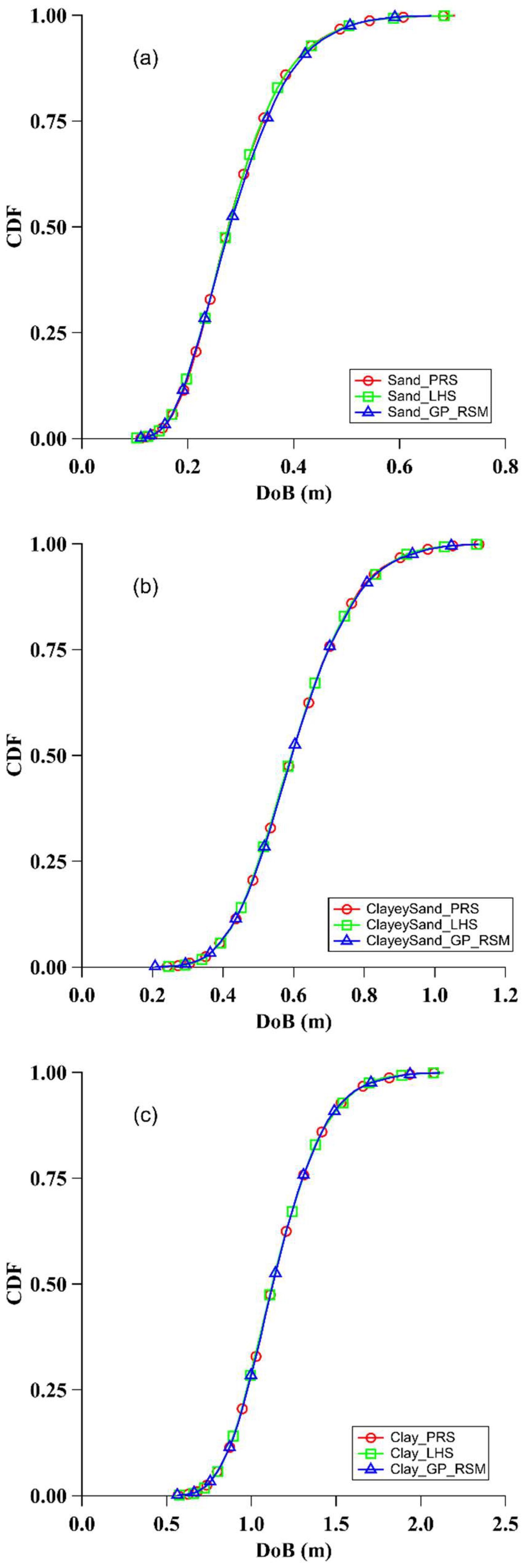
  • Various sampling techniques provide comparable predictions of the DoB, suggesting that all investigated methods are effective in capturing the uncertainties associated with the munitions’ burial depth. It has been noticed in all simulations that PRS and LHS consumed approximately similar run time, while the GP_RSM was the fastest sampling technique.
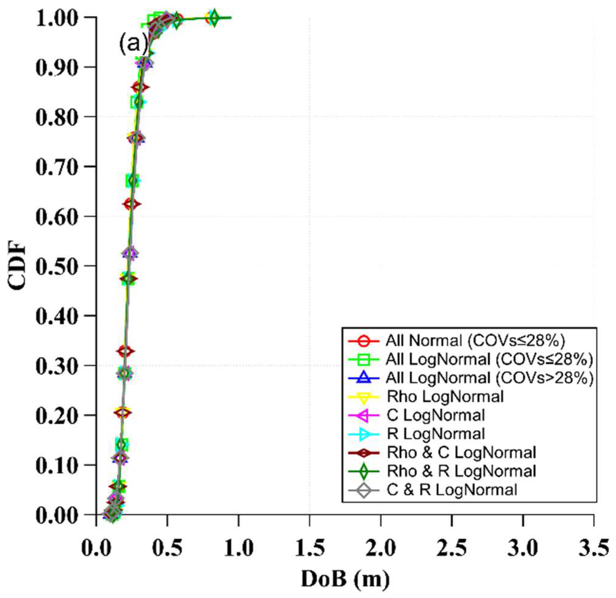
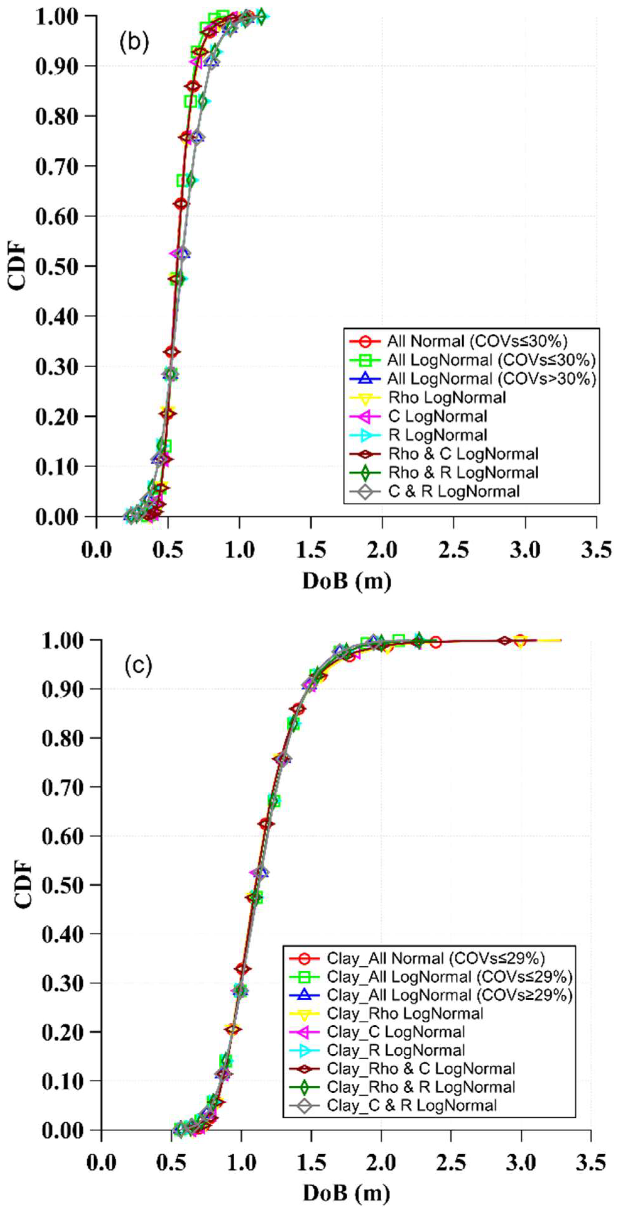
  • Sampling uncertainties from a normal or a lognormal distribution did not significantly impact the DoB predictions. However, the high uncertainties of the studied random variables resulted in normal distribution sampling physically inadmissible values for COVs above 28%. Thus, a lognormal distribution is preferred for use in sampling Poncelet drag and bearing coefficients when conducting probabilistic predictions of the DoB of unexploded UXOs.
  • Taking into account the inherent uncertainties associated with soil properties can have important impacts on the predicted DoB. The typical coefficient of variation in the DoB is approximately 32% in sand, 25% in clayey sand, and 22% in clay. These uncertainties can significantly influence the required cleanup depth for the redevelopment of sites afflicted by the presence of UXOs, with associated financial impacts on restoring former defense and battlefield sites.
  • The uncertainty of the density, drag coefficient, and bearing coefficient primarily influenced the depth of burial (DoB) in sandy soil, whereas in clayey sand soils, the uncertainty in the bearing coefficient was the dominant factor. In clayey soil, all variables under various distribution conditions resulted in approximately identical predictions, with no single variable appearing to be dominant.
The findings of this study contribute to enhancing the predictive capabilities and reliability of determining the depth of burial (DoB) for unexploded munitions (UXOs) in various soil types, crucial for the environmental cleanup of sites afflicted with UXOs. First, this work provides, for the first time, COVs for the drag and bearing parameters influencing the widely used Poncelet penetration model. In addition, the sensitivity analyses revealed the relative effects of drag and bearing coefficients on DoB predictions in different soils, which offers targeted guidance for soil characterization and optimizing data collection efforts.

Author Contributions

Conceptualization, M.O. and S.B.; Methodology, M.I.; Validation, M.I.; Formal analysis, B.N.M.; Investigation, M.O. and S.B.; Data curation, B.N.M.; Writing—original draft, B.N.M.; Writing—review & editing, M.I.; Visualization, B.N.M.; Supervision, M.I.; Project administration, M.I. and S.B.; Funding acquisition, M.I., M.O. and S.B. All authors have read and agreed to the published version of the manuscript.

Funding

This research was funded by Strategic Environmental Research and Development Program (SERDP) Project No. MR23-3855.

Data Availability Statement

The original contributions presented in this study are included in the article. Further inquiries can be directed to the corresponding author.

Acknowledgments

The authors gratefully acknowledge the support of the Strategic Environmental Research and Development Program (SERDP) Project No. MR23-3855. Analysis was carried out using NESSUS software (https://www2.swri.org/www2/nessus/register-acad.asp?_gl=1*yoyse7*_ga*MTQxNDUzOTQ2Ni4xNjg2NTkxMTY0*_ga_9QTX9F8GG4*MTY4NjU5MTE2My4xLjEuMTY4NjU5MTE4Ni4zNy4wLjA, accessed on 2 July 2024) developed by the Southwest Research Institute, as part of the NASA project titled “Probabilistic Structural Analysis Methods for Select Space Propulsion Components”.

Conflicts of Interest

The authors declare no conflict of interest.

References

  1. OSCE. The Impact of Mines, Unexploded Ordnance and Other Explosive Objects on Civilians in the Donetsk and Luhansk Regions of Eastern Ukraine, Report, Special Monitoring Mission to Ukraine, Organization for Security and Cooperation in Europe (OSCE). 2019. Available online: https://www.osce.org/ukraine-smm (accessed on 12 February 2025).
  2. Beran, L.; Zelt, B. Risk assessment for unexploded ordnance remediation. Stoch. Environ. Res. Risk Assess. 2015, 29, 1051–1061. [Google Scholar] [CrossRef]
  3. McKenna, S.A.; Pulsipher, B. Quantifying and reducing uncertainty in UXO site characterization. Stoch. Environ. Res. Risk Assess. 2009, 23, 153–154. [Google Scholar] [CrossRef]
  4. Ostrouchov, G.; Doll, W.E.; Beard, L.P.; Morris, M.D.; Wolf, D.A. Multiscale structure of UXO site characterization: Spatial estimation and uncertainty quantification. Stoch. Environ. Res. Risk Assess. 2009, 23, 215–225. [Google Scholar] [CrossRef]
  5. Roberts, B.L.; McKenna, S.A. The use of secondary information in geostatistical target area identification. Stoch. Environ. Res. Risk Assess. 2009, 23, 227–236. [Google Scholar] [CrossRef]
  6. Matzke, B.D.; Wilson, J.E.; Hathaway, J.E.; Pulsipher, B.A. Statistical algorithms accounting for background density in the detection of UXO target areas at DoD munitions sites. Stoch. Environ. Res. Risk Assess. 2009, 23, 181–191. [Google Scholar] [CrossRef]
  7. McKenna, S.A. UXO target area identification with hidden Markov models. Stoch. Environ. Res. Risk Assess. 2009, 23, 193–202. [Google Scholar] [CrossRef]
  8. Tantum, S.L.; Zhu, Q.; Torrione, P.A.; Collins, L.M. Modeling position error probability density functions for statistical inversions using a Goff–Jordan rough surface model. Stoch. Environ. Res. Risk Assess. 2009, 23, 155–167. [Google Scholar] [CrossRef]
  9. Walsh, S.; Anderson, K.; Hathaway, J.; Pulsipher, B. A Bayesian approach to monitoring and assessing unexploded ordnance remediation progress from munitions testing ranges. Stoch. Environ. Res. Risk Assess. 2011, 25, 805–814. [Google Scholar] [CrossRef]
  10. Robins, B. New Principles of Gunnery (Originially published in 1742). In Mathematical tracts of the Late Benjamin Ribins; Wilson, J., Ed.; Kessinger Publishing: London, UK, 1761; Volume 1, p. 341. [Google Scholar]
  11. Wang, W.; Wang, X.; Yu, G. Penetration depth of torpedo anchor in cohesive soil by free fall. Ocean Eng. 2016, 116, 286–294. [Google Scholar] [CrossRef]
  12. Wang, X.; Wang, H.; Liang, R.Y.; Zhu, H.; Di, H. A hidden Markov random field model based approach for probabilistic site characterization using multiple cone penetration test data. Struct. Saf. 2018, 70, 128–138. [Google Scholar] [CrossRef]
  13. Ads, A.; Bless, S.; Iskander, M. Shape effects on penetration of dynamically installed anchors in a transparent marine clay surrogate. Acta Geotech. 2023, 18, 3043–3059. [Google Scholar] [CrossRef]
  14. Raaj, S.K.; Saha, N.; Sundaravadivelu, R. Exploration of deep-water torpedo anchors-A review. Ocean Eng. 2023, 270, 113607. [Google Scholar] [CrossRef]
  15. Omidvar, M.; Iskander, M.; Bless, S. Response of granular media to rapid penetration. Int. J. Impact Eng. 2014, 66, 60–82. [Google Scholar] [CrossRef]
  16. Iskander, M.; Bless, S.; Omidvar, S. Rapid Penetration Into Granular Media: Visualizing the Fundamental Physics of Rapid Earth Penetration; Elsevier: Amsterdam, The Netherlands, 2015. [Google Scholar]
  17. Kim, Y.H.; Hossain, M.S.; Wang, D. Effect of strain rate and strain softening on embedment depth of a torpedo anchor in clay. Ocean Eng. 2015, 108, 704–715. [Google Scholar] [CrossRef]
  18. Liu, H.; Xu, K.; Zhao, Y. Numerical investigation on the penetration of gravity installed anchors by a coupled Eulerian–Lagrangian approach. Appl. Ocean Res. 2016, 60, 94–108. [Google Scholar] [CrossRef]
  19. White, R. Large Deformation Explicit Finite Element Simulations of High Strain Rate Loading and rapid Penetration of Clay; Manhattan College: Bronx, NY, USA, 2021. [Google Scholar]
  20. Phoon, K.-K. Role of reliability calculations in geotechnical design. Georisk Assess. Manag. Risk Eng. Syst. Geohazards 2017, 11, 4–21. [Google Scholar] [CrossRef]
  21. Phoon, K.-K. What Geotechnical Engineers Want to Know about Reliability. ASCE-ASME J. Risk Uncertain. Eng. Syst. Part A Civ. Eng. 2023, 9, 03123001. [Google Scholar] [CrossRef]
  22. Griffiths, D.V.; Zhu, D.; Huang, J.; Fenton, G.A. Observations on probabilistic slope stability analysis. In Proceedings of the 6th Asian-Pacific Symposium on Structural Reliability and Its Applications (APSSRA 2016), Shanghai, China, 28–30 May 2016. [Google Scholar]
  23. Zhang, J.; Zhang, L.M.; Tang, W.H. Bayesian Framework for Characterizing Geotechnical Model Uncertainty. J. Geotech. Geoenviron. Eng. 2009, 135, 932–940. [Google Scholar] [CrossRef]
  24. Zhang, J.; Tang, W.H.; Zhang, L.M.; Huang, H.W. Characterising geotechnical model uncertainty by hybrid Markov Chain Monte Carlo simulation. Comput. Geotech. 2012, 43, 26–36. [Google Scholar] [CrossRef]
  25. Wang, C.; Zhang, M.X.; Yu, G.L. Penetration depth of torpedo anchor in two-layered cohesive soil bed by free fall. China Ocean Eng. 2018, 32, 706–717. [Google Scholar] [CrossRef]
  26. Poncelet, J.V. Introduction Il la Mechanique Industrielle, 2nd ed.; Meline, Cans et Compagnie: Brussels, Belgium, 1839; p. 271. [Google Scholar]
  27. Kenneally, B.; Omidvar, M.; Bless, S.; Iskander, M. Observations of velocity-dependent drag and bearing stress in sand penetration. In Dynamic Behavior of Materials, Volume 1: Proceedings of the 2020 Annual Conference on Experimental and Applied Mechanics; Springer International Publishing: Cham, Switzerland, 2021; pp. 29–35. [Google Scholar]
  28. Thacker, B.H.; Riha, D.S.; Fitch, S.H.K.; Huyse, L.J.; Pleming, J.B. Probabilistic engineering analysis using the NESSUS software. Struct. Saf. 2006, 28, 83–107. [Google Scholar] [CrossRef]
  29. Bless, S.; Peden, B.; Guzman, I.; Omidvar, M.; Iskander, M. Poncelet Coefficients of Granular Media; Springer International Publishing: Cham, Switzerland, 2014; pp. 373–380. [Google Scholar] [CrossRef]
  30. Omidvar, M.; Bless, S.; Iskander, M. Recent Insights into Penetration of Sand and Similar Granular Materials. Shock. Phenom. Granul. Porous Mater. 2019, 2019, 137–163. [Google Scholar] [CrossRef]
  31. Tate, A. Further results in the theory of long rod penetration∗. J. Mech. Phys. Solids 1969, 17, 141–150. [Google Scholar] [CrossRef]
  32. Baecher, G.B.; Christian, J.T. Reliability and Statistics in Geotechnical Engineering; Wiley: Hoboken, NJ, USA, 2005. [Google Scholar]
  33. Das, B.M. (Ed.) . Geotechnical Engineering Handbook; J. Ross Publishing: New York, NY, USA, 2011. [Google Scholar]
  34. Lumb, P. Application of statistics in soil mechanics. In Soil Mechanics: New Horizons; Lee, I.K., Ed.; Newnes-Butterworth: London, UK, 1974; pp. 44–112. [Google Scholar]
  35. Mercurio, S.R.; Bless, S.; Ads, A.; Omidvar, M.; Iskander, M. Rate Dependence of Penetration Resistance in a Cohesive Soil. Society for Experimental Mechanics Annual Conference and Exposition; Springer Nature: Cham, Switzerland, 2023. [Google Scholar]
  36. Mercurio, S.R.; Iskander, M.; Omidvar, M.; Bless, S. Calibration of the Geoponcelet Penetration Model in Cohesive Soil. ASCE J. Geotech. Geoenviron. Eng. 2024; In Preparation. [Google Scholar]
  37. Omidvar, M.; Dinotte, J.; Giacomo, L.; Bless, S.; Iskander, M. Photon Doppler velocimetry for resolving vertical penetration into sand targets. Int. J. Impact Eng. 2024, 185, 104827. [Google Scholar] [CrossRef]
  38. Omidvar, M.; Dinotte, J.; Giacomo, L.; Bless, S.; Iskander, M. Dynamics of sand response to rapid penetration by rigid projectiles. Granul. Matter 2024, 26, 73. [Google Scholar] [CrossRef]
  39. He, R.; Wu, C.; Xing, X.; Li, J. Dependence Structures of Soil Parameters in Sandy Clay. ASCE-ASME J. Risk Uncertain. Eng. Syst. Part A Civ. Eng. 2021, 7, 05021005. [Google Scholar] [CrossRef]
  40. Mercurio, S.; Grace, D.; Bless, S.; Iskander, M.; Omidvar, M. Frequency-shifted photonic doppler velocimetry (PDV) for measuring deceleration of projectiles in soils. In Acta Geotechnica; Springer Nature: Cham, Switzerland, 2024. [Google Scholar] [CrossRef]
  41. Morkos, B.N.; White, R.; Omidvar, M.; Iskander, M.; Bless, S. Numerical Simulation of High-Speed Penetration of Munitions in Clay. In GSP 352: Geo-Congress 2024, Geotechnical Data Analysis and Computation; ASCE: New York, NY, USA, 2024; pp. 82–91. [Google Scholar] [CrossRef]
  42. Duncan, J.M. Factors of Safety and Reliability in Geotechnical Engineering. J. Geotech. Geoenviron. Eng. 2000, 126, 307–316. [Google Scholar] [CrossRef]
  43. Fenton, G.A.; Griffiths, D.V. Risk Assessment in Geotechnical Engineering; John Wiley & Sons: Hoboken, NJ, USA, 2008. [Google Scholar]
  44. Nadim, F. Tools and Strategies for Dealing with Uncertainty in Geotechnics. In Probabilistic Methods in Geotechnical Engineering; Springer: Vienna, Austria, 2007; pp. 71–95. [Google Scholar] [CrossRef]
  45. Nadarajah, S. A generalized normal distribution. J. Appl. Stat. 2005, 32, 685–694. [Google Scholar] [CrossRef]
  46. Forbes, C.; Evans, M.; Hastings, N.; Peacock, B. Statistical Distributions; John Wiley & Sons: Hoboken, NJ, USA, 2011. [Google Scholar]
  47. Ang, A.H.-S.; Tang, W.H. Probability Concepts in Engineering: Emphasis on Applications In Civil and Environmental Engineering; Wiley: Hoboken, NJ, USA, 1975; Volume 1. [Google Scholar]
  48. Griffiths, D.V.; Fenton, G.A. Probabilistic Methods in Geotechnical Engineering; Springer: Berlin/Heidelberg, Germany, 2007. [Google Scholar]
  49. Schmidt, A.F.; Finan, C. Linear regression and the normality assumption. J. Clin. Epidemiol. 2018, 98, 146–151. [Google Scholar] [CrossRef]
  50. Xiao, T.; Zhang, L.-M.; Li, X.-Y.; Li, D.-Q. Probabilistic Stratification Modeling in Geotechnical Site Characterization. ASCE-ASME J. Risk Uncertain. Eng. Syst. Part A Civ. Eng. 2017, 3, 04017019. [Google Scholar] [CrossRef]
  51. Fan, H.; Liang, R. Application of Monte Carlo Simulation to Laterally Loaded Piles. GeoCongress 2012, 2012, 376–384. [Google Scholar] [CrossRef]
  52. Fenton, G.A.; Griffiths, D.V. The Random Finite Element Method (RFEM) in Bearing Capacity Analyses. In Probabilistic Methods in Geotechnical Engineering; Springer: Vienna, Austria, 2007; pp. 295–315. [Google Scholar] [CrossRef]
  53. Ji, J.; Wang, L.P. Efficient geotechnical reliability analysis using weighted uniform simulation method involving correlated nonnormal random variables. J. Eng. Mech. 2022, 148, 06022001. [Google Scholar] [CrossRef]
  54. Li, X.; Chi, S.W.; Foster, C.D. Sensitivity analysis of a three-invariant plasticity model with different sampling algorithms. Int. J. Geotech. Eng. 2023, 17, 221–233. [Google Scholar] [CrossRef]
  55. Mckay, M.D.; Beckman, R.J.; Conover, W.J. A Comparison of Three Methods for Selecting Values of Input Variables in the Analysis of Output From a Computer Code. Technometrics 2000, 42, 55–61. [Google Scholar] [CrossRef]
  56. Helton, J.C.; Davis, F.J. Latin hypercube sampling and the propagation of uncertainty in analyses of complex systems. Reliab. Eng. Syst. Saf. 2003, 81, 23–69. [Google Scholar] [CrossRef]
  57. Loh, W.-L. On Latin hypercube sampling. Ann. Stat. 1996, 24, 62310. [Google Scholar] [CrossRef]
  58. Kang, F.; Han, S.; Salgado, R.; Li, J. System probabilistic stability analysis of soil slopes using Gaussian process regression with Latin hypercube sampling. Comput. Geotech. 2015, 63, 13–25. [Google Scholar] [CrossRef]
  59. Toufigh, V.; Pahlavani, H. Probabilistic-Based Analysis of MSE Walls Using the Latin Hypercube Sampling Method. Int. J. Geomech. 2018, 18, 04018109. [Google Scholar] [CrossRef]
  60. Olsson, A.M.J.; Sandberg, G.E. Latin Hypercube Sampling for Stochastic Finite Element Analysis. J. Eng. Mech. 2002, 128, 121–125. [Google Scholar] [CrossRef]
  61. Riha, D.; Bichon, B.; Mcfarland, J.; Fitch, S. NESSUS Users’ Manual; Elsevier: Amsterdam, The Netherlands, 2015. [Google Scholar]
  62. Wang, D.; Ye, X.; Zheng, X. The scaling and dynamics of a projectile obliquely impacting a granular medium. Eur. Phys. J. E 2012, 35, 7. [Google Scholar] [CrossRef]
  63. Zhang, X.; Zhao, H.; Cheng, H.; Wang, X.; Zhang, D. The force and dynamic response of low-velocity projectile impact into 3D dense wet granular media. Powder Technol. 2024, 434, 119309. [Google Scholar] [CrossRef]
Figure 1. Vertical penetration of 60° cone projectile in soils.
Applsci 15 03259 g001
Figure 2. Typical normal and lognormal distributions of bearing coefficient in sand with μ = 0.94 MPa and COV = 58%.
Applsci 15 03259 g002
Figure 3. CDFs of DoB in sand using: (a) Restrict Normal Distribution to COV Values Lower than 30%, (b) Restrict Lognormal Distribution to COV Values Lower than 30%, (c) Unrestrict Lognormal Distribution, and (d) Use of Mixed Normal and Lognormal Distributions.
Applsci 15 03259 g003
Figure 4. CDFs of DoB in clayey sand using: (a) Restrict Normal Distribution to COV Values Lower than 30%, (b) Restrict Lognormal Distribution to COV Values Lower than 30%, (c) Unrestrict Lognormal Distribution, and (d) Use of Mixed Normal and Lognormal Distributions.
Applsci 15 03259 g004
Figure 5. CDFs of DoB in clay using: (a) Restrict Normal Distribution to COV Values Lower than 30%, (b) Restrict Lognormal Distribution to COV Values Lower than 30%, (c) Unrestrict Lognormal Distribution, and (d) Use of Mixed Normal and Lognormal Distributions.
Applsci 15 03259 g005aApplsci 15 03259 g005b
Figure 6. Comparison of CDFs of DoB in (a) sand, (b) clayey sand, and (c) clay using a variety of distributions.
Applsci 15 03259 g006aApplsci 15 03259 g006b
Figure 7. CDFs of DoB using different sampling techniques for (a) sand, (b) clayey sand, and (c) clay.
Applsci 15 03259 g007
Table 1. Summary of Variables and Uncertainties Employed in the Poncelet Model.
Soil TypeRandom VariableRangeMean ( μ )COV (%)
Dry Sand
[37,38]
Density ( ρ ) (gm/cm3)1.57–1.821.736
Poncelet Drag ( C )0.84–1.681.2333
Poncelet Bearing Resistance ( R ) (MPa)0.40–1.780.9458
Clayey Sand
[35,36,40]
Density ( ρ ) (gm/cm3)1.78–1.851.811
Poncelet Drag ( C )0.21–0.320.2514
Poncelet Bearing Resistance ( R ) (MPa)0.62–3.381.7366
Clay
[19,41]
Density ( ρ ) (gm/cm3)1.810
Poncelet Drag ( C )0.0529
Poncelet Bearing Resistance ( R ) (MPa)2.2529
ProjectileMass ( M ) (gm)35(Deterministic)
Diameter ( D ) (mm)14.3(Deterministic)
Impact Velocity ( V i ) (m/s)200(Deterministic)
Table 2. Conditions for investigating the effect of selected distributions on DOB.
ConditionVariablesDistributionSand
COV
(%)
Clayey Sand
COV
(%)
Clay
COV
(%)
ρCRρCRρCR
1ρ, C, RNormal102828101430102927
2ρ, C, RLognormal102828101430102927
3ρ, C, RLognormal103358101466102929
4C, RNormal282814302927
ρLognormal101010
5ρ, RNormal102810301027
CLognormal331429
6ρ, CNormal102810141029
RLognormal586629
7RNormal283027
ρ, CLognormal103310141029
8CNormal281429
ρ, RLognormal105810661029
9ρNormal101010
C, RLognormal335814662929
Table 3. One-way ANOVA results.
F-StatisticFc P
Sand0.731.960.67
Clayey Sand0.191.960.99
Clay0.421.960.9
Table 4. Uncertainties in predicted DoB in sand, clayey sand, and clay.
Sampling
Method
Mean DoB
m
R a n g e   o f   C O V
%
A v e r a g e   C O V
%
Computational Effort
SandPRS0.2827–3431100%
LHS0.2827–3631105%
GP_RSM0.2828–373235%
Clayey SandPRS0.6022–2624100%
LHS0.6022–2724102%
GP_RSM0.6022–272536%
ClayPRS1.1319–2422100%
LHS1.1219–2421103%
GP_RSM1.1319–242237%
Disclaimer/Publisher’s Note: The statements, opinions and data contained in all publications are solely those of the individual author(s) and contributor(s) and not of MDPI and/or the editor(s). MDPI and/or the editor(s) disclaim responsibility for any injury to people or property resulting from any ideas, methods, instructions or products referred to in the content.

