Explicit-Time Trajectory Tracking for a State-Constraint Continuum Free-Floating Space Robot with Smooth Joint-Path and Low Input

Abstract

For the problem of large joint angular velocity and high input in the trajectory planning and control of robots, an explicit-time trajectory tracking for a state-constraint continuum free-floating space robot with smooth joint-path and low input is proposed. Employing the piecewise constant curvature (PCC) assumption as the modeling foundation for the continuum space robot and utilizing modified Rodriguez parameters (MRPs) to describe attitude errors, a pose error feedback kinematic model for the continuum space robot is established. Based on the Lagrangian method, a dynamic model for the continuum space robot is developed. Explicit time theory and pose feedback methods are employed for the trajectory planning of the continuum space robot. Using explicit time theory and sliding mode control, tracking control for the planned joint trajectory is conducted. The Lyapunov theory is utilized to demonstrate the convergence of the system tracking error within the explicit time. Finally, the combination of trajectory planning and tracking control enhances the control performance of the continuum space robot. Simulation results validate the effectiveness of the proposed methods.

1. Introduction

With the development of space exploration in recent decades, on-orbit space robots are increasingly gaining attention from researchers. Space robots serve as crucial tools for ensuring the safe operation and prolonged lifespan of spacecraft, contributing to tasks such as space station construction, satellite maintenance, and space debris clearance [1,2]. However, traditional rigid robots, characterized by limited degrees of freedom and insufficient flexibility, face challenges in efficiently and safely while completing on-orbit tasks within complex and confined environments. Continuum robots, as a new type of biomimetic robotic arm, offer higher flexibility and enhanced interactive safety [3]. They can perform a variety of tasks in narrow and restricted environments, holding promising applications in the field of space robots.

Continuum robots can achieve continuous bending and motion in complex and confined unstructured environments, leveraging their inherent flexibility. The driving mechanism of continuum manipulators is mostly installed in the base at the bottom. With a relatively small mass and lower stiffness compared to traditional rigid robots, continuum robots exhibit higher safety when in contact with the environment. Currently, continuum robots find widespread applications in areas such as aerospace [4], medical fields [5], power systems [6], exploration [7], and rescue operations [8]. However, the use of soft materials and structures can lead to vibrations, creating a strongly coupled nonlinear system. Modeling and controlling such systems both still lack a well-established unified approach. Additionally, the base of space robots is free-floating, introducing complex dynamic coupling between the motion of the manipulator and the satellite base, posing significant challenges in trajectory planning [9]. Currently, research either focuses solely on the trajectory planning problem of continuum space robots or solely on the dynamic tracking control problem, without effectively integrating the two. Therefore, research on the kinematics and dynamics of continuum space robots is meaningful but also confronts various challenges [10]. Inaccurate calculation of the robot system’s motion deformation, kinetic energy, and momentum can affect the dynamic coupling of the base, thereby increasing trajectory planning and control errors.

Current commonly used high-precision control methods for robots include adaptive control, fuzzy control, sliding mode control, backstepping control, etc., but most of these systems are asymptotically stable. Dian et al. [6], addressing the uncertainty compensation issue in a cable-driven continuum robot system, proposed a novel disturbance-resistant control method based on a sliding mode controller and a linear extended state observer. While this method can compensate for the effects of system uncertainty, its sliding mode controller employs exponential reaching law, which cannot guarantee the convergence time of errors. Ayala-Carrillo et al. [11], addressing robust tracking control issues in pneumatic-driven continuum soft robots, proposed a finite-time sliding mode controller to achieve convergence of tracking errors within a finite time. For the task space tracking control problem of free-floating space robots, Jin et al. [12] utilized a fixed-time extended state observer to ensure that, even in the presence of external disturbances, the convergence time of tracking errors is bounded and independent of the system’s initial state. Since the relationship between fixed-time controller time and parameters is complex, Sanchez-Torres et al. [13] introduced the predefined time stability theory, with the upper bound of stability time related to the system, allowing for the pre-definition and simplification of controller design.

The predefined time stability theory ensures system response speed and allows for specification of the convergence time during controller design. Ye et al. [14] proposed an attitude tracking controller for rigid spacecraft based on predefined time, combining sliding mode control and predefined time theory to achieve high-precision control of spacecraft attitude. Jin et al. [15], addressing the tracking control problem of free-floating space robots in the task space, introduced a predefined time-based backstepping control method, enabling the end-effector position and attitude of the robot to track the desired trajectory within a predetermined time, even with initial errors. Liu et al. [16] presented a predefined time-based terminal sliding mode control method, demonstrating through rigorous mathematical formulation the system’s singularity-free and globally predefined time convergence. This method achieves high-precision trajectory tracking control for dual-arm space robots. However, this work did not further investigate the trajectory planning problem considering kinematics. However, predefined-time control methods can guarantee convergence of errors within a given time in any situation, but they lead to the requirement of larger input gains. This is because the predefined-time theory considers convergence time even from infinitely large initial states, leading to overly conservative estimates of convergence time. In trajectory planning, a higher input gain represents larger joint angular velocities, which can lead to increased vibration for continuum space robots. In trajectory tracking control, traditional predefined time inputs that are relatively large can cause actuator saturation and faults.

In engineering applications, it is rare for system states to tend towards infinity; most of the time, they are bounded. For the case where the initial conditions are bounded, Yan et al. [17] proposed a generalized explicit time stability system with bounded gains, which significantly reduces the initial control input. However, there is currently relatively little research on specific applications based on explicit time stability. The control theory can achieve system convergence within predefined time while initiating smaller initial control inputs to reduce the damage caused by excessive control inputs to the actuators. However, in designing controllers, the mathematical expression forms are complex, especially when applied to sliding mode control, making it difficult to derive. Research on how to design more concise and practical trajectory planning and control algorithms based on explicit time theory is still needed. In summary, this paper proposes a high-precision control scheme for trajectory planning and tracking control of a continuum space robot. By employing explicit time theory in trajectory planning and tracking for continuous space robots, smoother joint trajectories and smaller initial control inputs can be obtained. The main contributions of this paper are as follows:

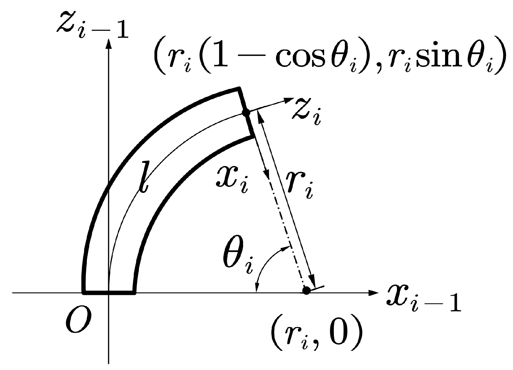
(1) The model of continuum space robots is established by introducing the arc length parameter. Based on this, the pose feedback kinematic model of continuous space robots is established using quaternions to describe the end effector’s pose of the robotic arm. In the modeling process, the momentum conservation and nonholonomic constraints of the robotic system are taken into account. This modeling approach has more accurate model parameters.

(2) Based on the kinematic model of the continuum space robot, a trajectory planning method utilizing explicit time stability theory is proposed. Compared to other methods, this approach can generate smoother joint trajectories.

(3) Building upon the dynamic model of the continuum space robot, a trajectory tracking control method is devised that integrates explicit time stability theory and sliding mode control. This trajectory tracking control method achieves high-precision tracking of the desired trajectory within explicit time. Compared to other methods, this approach requires lower control inputs.

(4) The proposed trajectory planning and tracking control methods can be combined to further enhance the control performance of continuum space robots. Consequently, this enables high-precision trajectory planning and control for continuum space robots.

(5) Experiments were conducted on a fixed-base, single-end continuum robot, confirming the effectiveness of the explicit-time algorithm on a physical system.

In the subsequent sections, Section 2 presents the three-dimensional model of the continuum space robot. Section 3 establishes the theoretical groundwork for the robot’s motion control in later parts of the paper. Section 4 provides the foundational model. Section 5 covers the kinematic and dynamic models. Section 6 introduces trajectory planning and control methods based on explicit time stability. Section 7 covers the simulation and analysis of the proposed methods. Section 8 perform experimental validation. Section 9 presents the conclusion. Finally, Section 10 presents future recommendations.

2. Notion

Continuum space robots consists of a satellite base and a continuum manipulator.

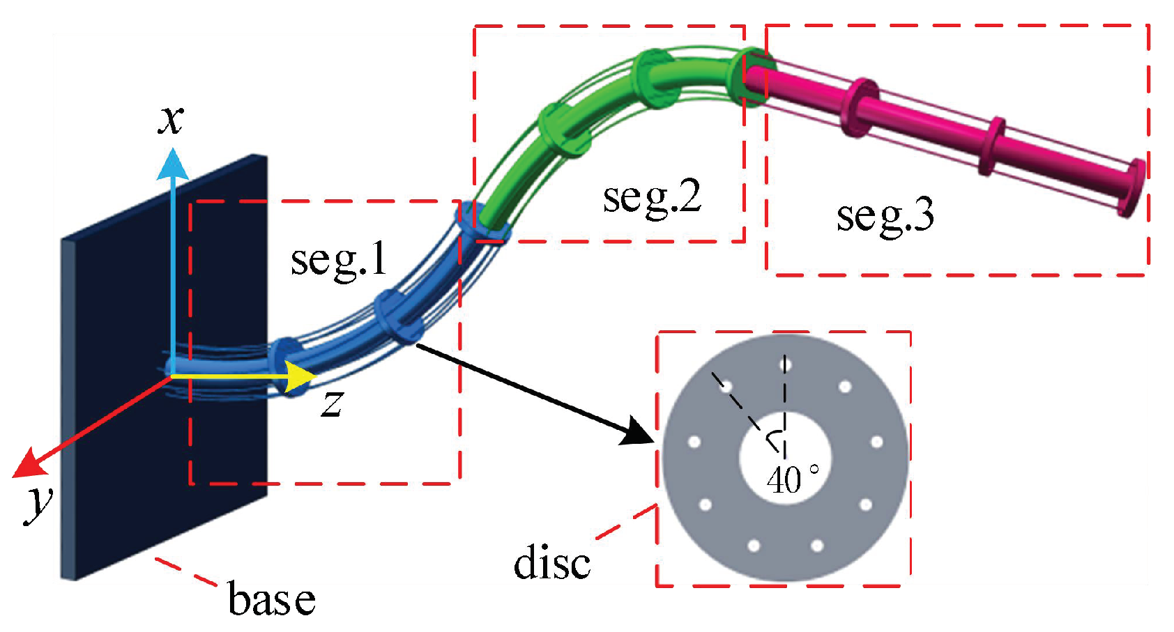
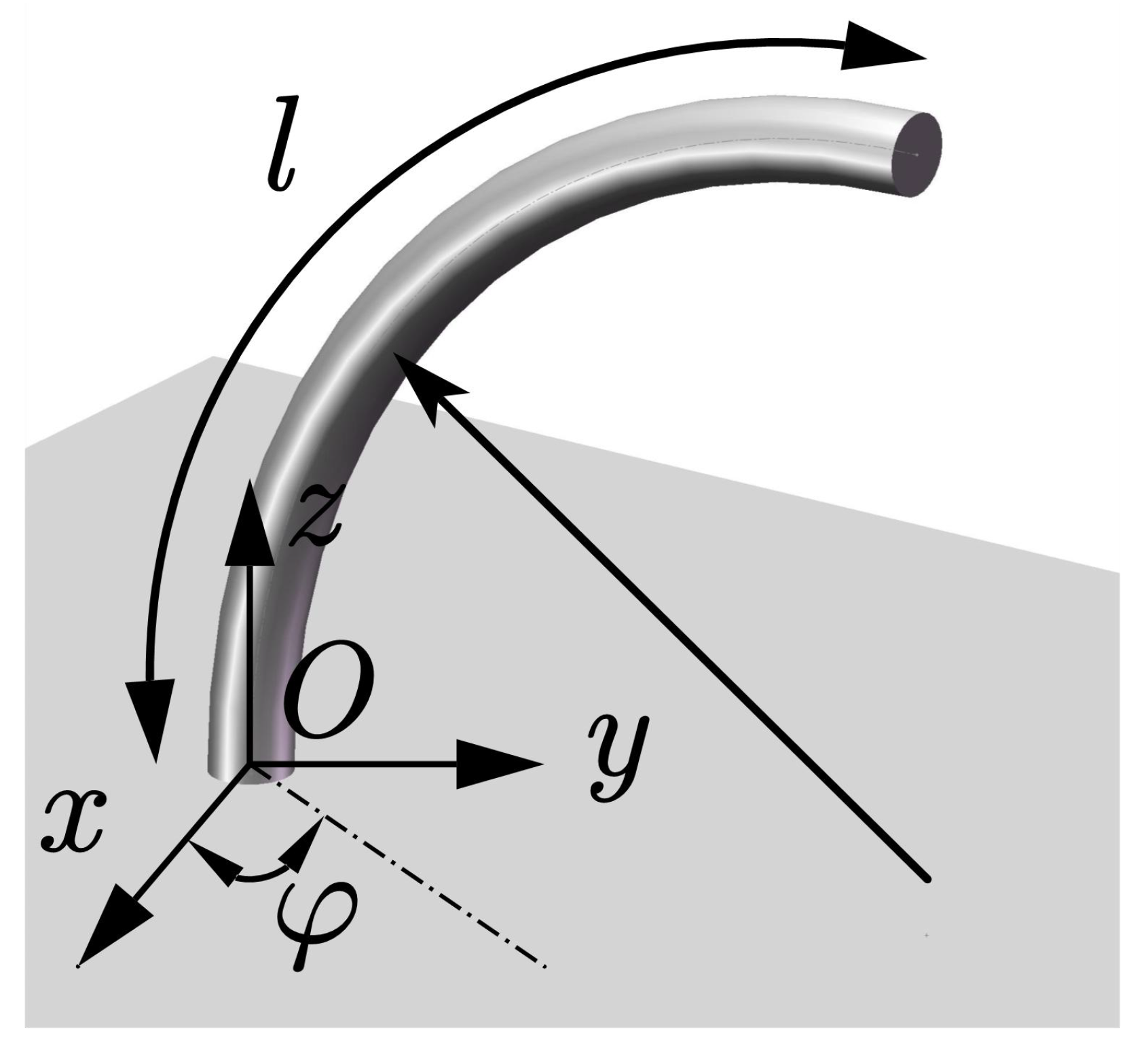
The three-dimensional model of the continuum manipulator is depicted in Figure 1, comprising a three-segment, cable-driven continuum manipulator. Each segment has a fixed length, with a central axis consisting of an elastic flexible rod controlled by three driving cables, allowing it to bend in any direction, forming an arc. The first segment passes through 9 cables, the second through 6, and the third through 3. Equally spaced support discs are employed to maintain the curvature of the central rod, with the number of perforations on each disc matching the number of cables passing through each segment. Actuated by motors on the base, the cables are pulled to induce bending deformation in the manipulator, facilitating pose control of the robotic system.

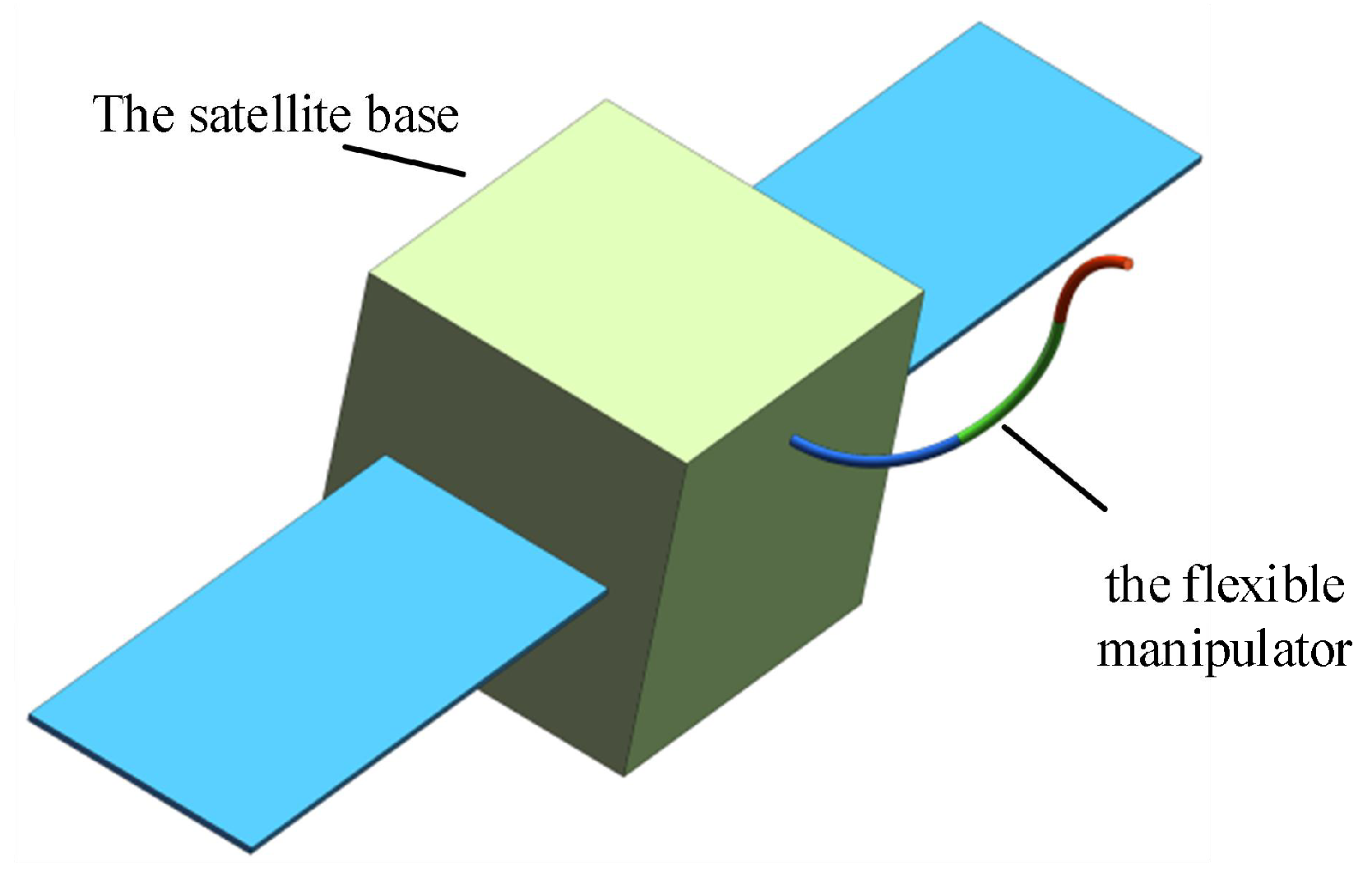
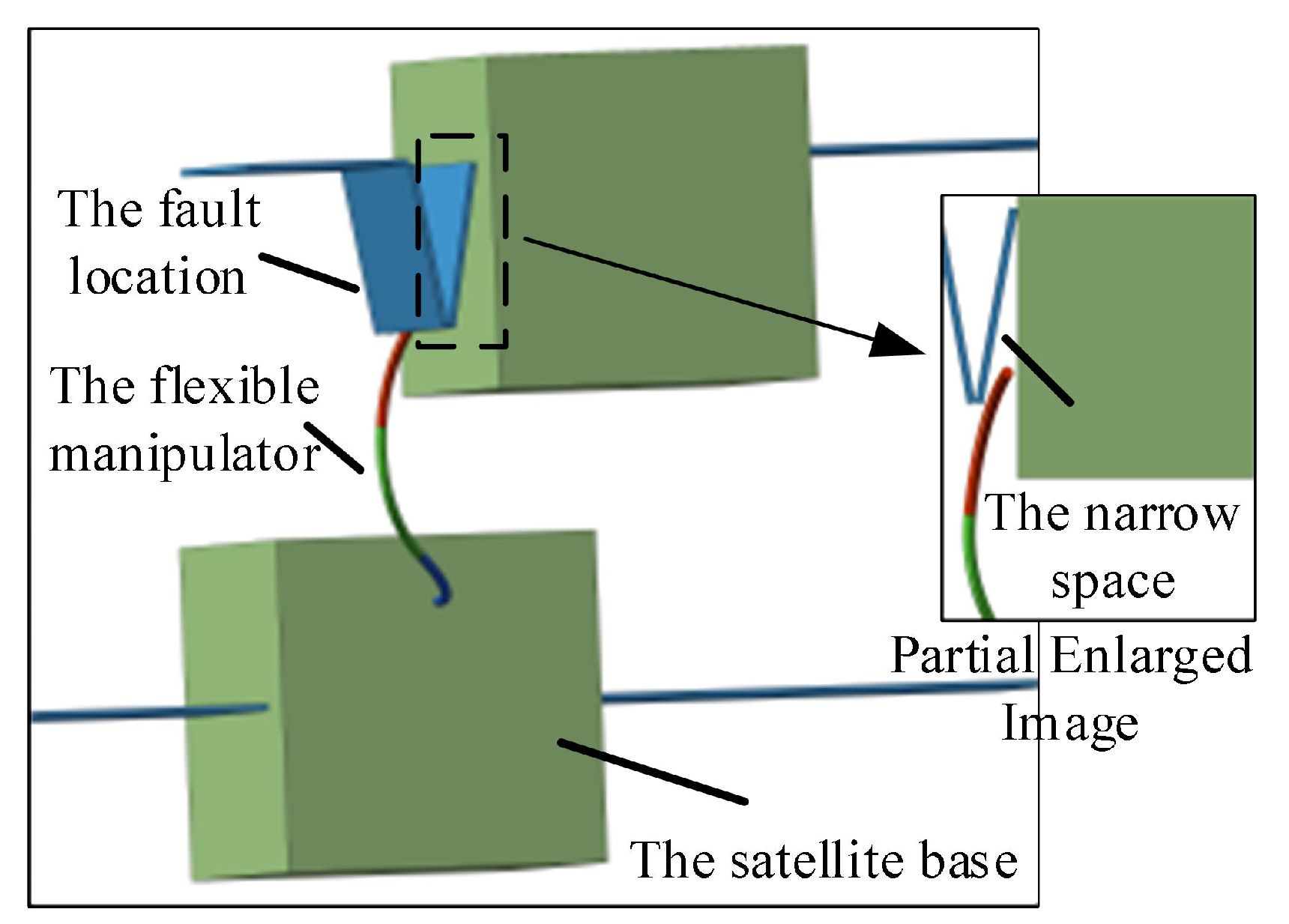
The three-dimensional model of the continuum space robot system is illustrated in Figure 2. The base is a free-floating satellite, and the manipulator is a continuum manipulator. The advantages of this configuration lie in the flexibility and adaptability of the cable-driven continuum manipulator, making it more suitable for exploration and operations in complex and space-constrained environments, as depicted in Figure 3.

Define the symbols as follows: ${\mathit{q}}_0={\left[\begin{array}{cccccc}{x}_0& y_0& z_0& {\phi }_0& {\theta }_0& {\psi }_0\end{array}\right]}^{\mathrm{T}}$ is the virtual joint variable corresponding to the base, where ${\mathit{r}}_0={\left[\begin{array}{ccc}{x}_0& y_0& z_0\end{array}\right]}^{\mathrm{T}}$ is the coordinates of the center of mass of the base in the inertial frame and ${\left[\begin{array}{ccc}{\phi }_0& {\theta }_0& {\psi }_0\end{array}\right]}^{\mathrm{T}}$ is the Euler angles describing the orientation of the base relative to the inertial frame, using a 3-2-1 sequence. ${\mathit{V}}_0={\left[\begin{array}{cc}{\mathit{v}}_0^{\mathrm{T}}& {\mathit{\omega }}_0^{\mathrm{T}}\end{array}\right]}^{\mathrm{T}}$ is the velocity of the base. $\mathit{q}={\left[{\phi }_1{\theta }_1{\phi }_2{\theta }_2{\phi }_3{\theta }_3\right]}^{\mathit{T}}$ is the joint variable, where ${\phi }_i$ and ${\theta }_i$ are the bending plane angle and bending angle of the i-th (i = 1, 2, 3) segment of the continuum manipulator. $\dot{\mathit{q}}$ is the joint velocity. $\overline{\mathit{q}}={\left[{\mathit{q}}_0^{\mathrm{T}}{\mathit{q}}^{\mathrm{T}}\right]}^{\mathrm{T}}$ is the generalized virtual joint variable. $\dot{\overline{\mathit{q}}}$ is the generalized virtual joint velocity. ${\mathit{P}}_{\mathbf{0}}$ and ${\mathit{L}}_{\mathbf{0}}$ are the linear momentum and angular momentum of the base, respectively. ${\mathit{P}}_{\mathit{i},\mathit{d}}$, ${\mathit{L}}_{\mathit{i},\mathit{d}}$, ${\mathit{P}}_{\mathit{i},\mathit{r}}$, and ${\mathit{L}}_{\mathit{i},\mathit{r}}$ are the linear momentum and angular momentum of the elastic rod and support disk of the i-th segment of the continuum robot, respectively.

${\mathit{M}}_{\mathbf{0}\mathit{t}}$ and ${\mathit{M}}_{\mathbf{0}\mathit{r}}$ are the inertia matrices for translation and rotation of the base, respectively. ${\mathit{M}}_{\mathit{i},\mathit{dt}}$, ${\mathit{M}}_{\mathit{i},\mathit{dr}}$, ${\mathit{M}}_{\mathit{i},\mathit{rt}}$, and ${\mathit{M}}_{\mathit{i},\mathit{rr}}$ are the inertia matrices for the translation and rotation of the elastic rod and support disk of the i-th segment of the continuum robot, respectively.

3. Preliminaries

3.1. Deformation Description of the Continuum Robot

Common methods for describing the deformation of the continuum manipulator include the constant curvature method, finite element method, and Cosserat rod theory. To simplify the modeling process and focus on the control of the continuum manipulator, the constant curvature method is chosen as the foundation for kinematic modeling. According to the PCC assumption, a continuous robot can be approximated as a series of subsegments with uniform curvature.

For a segment of a continuum manipulator with a length of l, as illustrated in Figure 4, its motion deformation can be described as a section of rod with constant curvature [18].

Define the rotational transformation as:

$$R_z\left({\phi }_i\right)=\left[\begin{array}{ccc}{c}_{{\phi }_i}& -s_{{\phi }_i}& 0\\ s_{{\phi }_i}& c_{{\phi }_i}& 0\\ 0& 0& 1\end{array}\right],R_y\left({\theta }_i\right)=\left[\begin{array}{ccc}{c}_{{\theta }_i}& 0& s_{{\theta }_i}\\ 0& 1& 0\\ -s_{{\theta }_i}& 0& c_{{\theta }_i}\end{array}\right]$$

(1)

where c represents cos and s represents sin.

Define the angle between the plane containing a single segment of the continuum manipulator’s arc and the plane $xOz$ as the curvature plane angle $\phi$, as illustrated in Figure 5. The i-th segment of the continuum manipulator, when ${\phi }_i=0$, is depicted in Figure 6.

In Figure 6, ${\theta }_i$ is the angle formed by $x_i$ and $x_{i-1}$, ${\theta }_i$ is defined as the bending angle for the i-th segment, and $r_i$ is the bending radius for the i-th segment. From Figure 6, the local position of the end of this segment after bending can be obtained.

$$\begin{array}{cc}\hfill {\mathit{r}}_{i,lcl}& ={\left[(1-c_{{\theta }_i})0s_{{\theta }_i}\right]}^{\mathrm{T}}{r}_i\hfill \\ \hfill & ={\left[(1-c_{{\theta }_i})0s_{{\theta }_i}\right]}^{\mathrm{T}}{\displaystyle \frac{l}{{\theta }_i}}\hfill \end{array}$$

(2)

where the subscript _lcl represents in the local coordinate system. When ${\mathit{r}}_{i,lcl}={\left[\begin{array}{ccc}0& 0& l\end{array}\right]}^T$.

To obtain the pose of every point on the continuum manipulator, it is proposed to use the arc length parameter for modeling. Consider a segment of the continuum manipulator as an arc, define the arc length parameter $s\in [0,1]$, where $s=0$ corresponds to the beginning of the arc and $s=1$ corresponds to the end of the arc. When ${\theta }_i=0$, ${\mathit{r}}_{i,lcl}={\left[\begin{array}{ccc}0& 0& sl\end{array}\right]}^T$. Under the PCC assumption, the position coordinates of any point in the arm segment can be expressed as

$$\begin{array}{cc}\hfill {\mathit{r}}_{i,lcl}({\theta }_i,s)& ={\left[(1-c_{s{\theta }_i})0s_{s{\theta }_i}\right]}^{\mathrm{T}}{\displaystyle \frac{l}{{\theta }_i}}\hfill \\ \hfill & \triangleq \mathit{p}({\theta }_i,s)\hfill \end{array}$$

(3)

When the curvature plane angle ${\phi }_i\ne 0$, the position of any point in the i-th segment of the robotic arm in the local coordinates of the i-th segment can be represented as

$$\begin{array}{c}\hfill {\mathit{r}}_{i,\mathit{lcl}}({\phi }_i,{\theta }_i,s)={\mathit{R}}_z\left({\phi }_i\right)\mathit{p}({\theta }_i,s)\end{array}$$

(4)

Attitude can be represented by a rotation transformation matrix [19] as

$$\begin{array}{cc}\hfill {\mathit{R}}_{i,lcl}({\phi }_i,{\theta }_i,s)& ={\mathit{R}}_z\left({\phi }_i\right){\mathit{R}}_y\left(s{\theta }_i\right){\mathit{R}}_z(-{\phi }_i)\hfill \end{array}$$

(5)

In practical applications, adjusting the flexibility of a continuum manipulator and adapting to various complex scenarios can be achieved by concatenating several subsegments, enhancing the flexibility at the robot system.

3.2. Kinematic Analysis of the Continuum Robot

The continuum manipulator studied in this paper consists of three segments. To maintain generality, assume a total of n segments, and here $n=3$.

The arc length parameter of the i-th $(i=1,2,\dots ,n)$ segment is and the absolute position at the axis center is

$$\begin{array}{c}\hfill {\mathit{r}}_i(·,s)={\mathit{r}}_{i-1}(·,1)+{\mathit{R}}_{i-1}{\mathit{R}}_z\left({\phi }_i\right)\mathit{p}({\theta }_i,s)\end{array}$$

(6)

where · in ${\mathit{r}}_i(·,s)$ represents other independent variable parameters. Subsequently, for the sake of symbol simplicity, only arc length parameters will be provided for independent variables, disregarding other variables that include the arc length parameters. For example, ${\mathit{r}}_i(·,s)$ will be further abbreviated as ${\mathit{r}}_i\left(s\right)$. Also, ${\mathit{r}}_0\left(1\right)$ is equivalent to ${\mathit{r}}_0$, and similar expressions will not be elaborated in the following text.

Considering the offset between the installation position of the manipulator and the base, the absolute position at the axis center for the first segment with an arc length parameter of s is

$$\begin{array}{c}\hfill {\mathit{r}}_1\left(s\right)={\mathit{r}}_0+{\mathit{R}}_0(\mathit{b}+{\mathit{R}}_z\left({\phi }_1\right)\mathit{p}({\theta }_1,s))\end{array}$$

(7)

where $\mathit{b}$ represents the installation position on the base for the first segment of the continuum manipulator. This position corresponds to the coordinates of the intersection point between the base and the central axis of the first segment in the fixed coordinate system of the base.

The rotation matrix representing the transformation from the local coordinate system at the section with an arc length parameter of s in the i-th segment to the inertial coordinate system is given by

$$\begin{array}{c}\hfill {\mathit{R}}_i\left(s\right)={\mathit{R}}_{i-1}\left(1\right){\mathit{R}}_z\left({\phi }_i\right){\mathit{R}}_y\left(s{\theta }_i\right){\mathit{R}}_z(-{\phi }_i)\end{array}$$

(8)

This matrix represents the orientation of the section relative to the inertial system.

The absolute linear velocity at the axis center of the i-th segment with an arc length parameter of s is given by

$$\begin{array}{cc}\hfill {\mathit{v}}_i\left(s\right)& ={\mathit{v}}_{i-1}\left(1\right)+{\mathit{\omega }}_{i-1}\left(1\right)\times {\mathit{r}}_{i-1,i}\left(s\right)\hfill \\ \hfill & +{\mathit{R}}_{i-1}\left(1\right){\mathit{R}}_z\left({\phi }_i\right)\mathit{p}(s,{\theta }_i){\dot{\phi }}_i\hfill \\ \hfill & +{\mathit{R}}_{i-1}\left(1\right){\mathit{R}}_z\left({\phi }_i\right){\mathit{p}}_{{\theta }_i}({\theta }_i,s){\dot{\theta }}_i\hfill \\ \hfill & ={\mathit{J}}_{i,v}\left(s\right)\dot{\overline{\mathit{q}}}\hfill \end{array}$$

(9)

where ${\mathit{r}}_{i-1,i}\left(s\right)={\mathit{r}}_i\left(s\right)-{\mathit{r}}_{i-1}\left(1\right)$ is the position vector from the end of the $(i-1)$-th segment to the position in the i-th segment with an arc length parameter of s, × denotes the cross product, ${{\mathit{R}}_{z,}}_{{\phi }_i}$ is $\partial {\mathit{R}}_z\left({\phi }_i\right)/\partial {\phi }_i$, ${\mathit{p}}_{{\theta }_i}({\theta }_i,s)$ is $\partial \mathit{p}({\theta }_i,s)/\partial {\theta }_i$, and ${\mathit{J}}_{i,v}\left(s\right)$ is the corresponding linear velocity Jacobian matrix.

The absolute angular velocity at the axis center of the i-th segment with an arc length parameter of s is given by

$$\begin{array}{cc}\hfill {\mathit{\omega }}_i\left(s\right)& ={\mathit{\omega }}_{i-1}\left(1\right)\hfill \\ \hfill & +{\mathit{R}}_{i-1}\left[{\mathit{e}}_3{\dot{\phi }}_i+{\mathit{R}}_z\left({\phi }_i\right){\mathit{e}}_{2}s{\dot{\theta }}_i-{\mathit{R}}_z\left({\phi }_i\right){\mathit{R}}_y\left(s{\theta }_i\right){\mathit{e}}_3{\dot{\phi }}_i\right]\hfill \\ \hfill & ={\mathit{J}}_{i,\omega }\left(s\right)\dot{\overline{\mathit{q}}}\hfill \end{array}$$

(10)

where ${\mathit{J}}_{i,\omega }\left(s\right)$ is the corresponding angular velocity Jacobian matrix.

The linear momentum of the support disk for the i-th segment of the continuum manipulator is given by

$$\begin{array}{c}\hfill {\mathit{P}}_{i,d}=\sum _{j=1}^{n_1}{m}_d{\mathit{v}}_i(j/n_1)\end{array}$$

(11)

where $m_d$ is the mass of the disk and j is the j-th support disk on the continuum manipulator, where j ranges from 1 to the total number $n_1$ of support disks on the i-th segment of the continuum manipulator.

The angular momentum of the support disk for the i-th segment of the continuum manipulator is given by

$$\begin{array}{c}\hfill {\mathit{L}}_{i,d}=\sum _{j=1}^{n_1}{\left[{\mathit{R}}_i\left(s\right){\mathbb{I}}_d{\mathit{R}}_{\mathrm{i}}^{\mathrm{T}}\left(s\right){\mathit{\omega }}_i\left(s\right)\right]}_{s=j/n_1}\end{array}$$

(12)

where ${\mathbb{I}}_d$ is the moment of inertia of the disk in its own body coordinate system.

The linear momentum of the central elastic rod for the i-th segment of the continuum manipulator is given by

$$\begin{array}{c}\hfill {\mathit{P}}_{i,r}={\int }_0^1\rho {\mathit{v}}_i\left(s\right)Alds\end{array}$$

(13)

where $\rho$ is the density of the elastic rod and A is the cross-sectional area of the elastic rod.

The linear momentum of the central elastic rod for the i-th segment of the continuum manipulator is given by

$$\begin{array}{c}\hfill {\mathit{L}}_{i,r}={\int }_0^1{\mathit{R}}_i\left(s\right){\mathbb{I}}_r{\mathit{R}}_i^{\mathrm{T}}\left(s\right){\mathit{\omega }}_i\left(s\right)lds\end{array}$$

(14)

where ${\mathbb{I}}_r$ is the moment of inertia of a segment of the elastic rod with length $lds$ in its own body coordinate system. For simulation purposes and to improve computational efficiency, the integration calculation for the continuous elastic rod can be simplified by discretizing it into several small segments and then summing them up. Therefore, Equation (14) can be modified to

$$\begin{array}{c}\hfill {\mathit{L}}_{i,r}\approx {\displaystyle \frac{1}{n_2}}\sum _{j=0}^{n_2-1}{\left[{\mathit{R}}_i\left(s\right){\mathbb{I}}_r{\mathit{R}}_i^T\left(s\right){\mathit{\omega }}_i\left(s\right)l\right]}_{s=\frac{1}{2n_2}+\frac{j}{n_2}}\end{array}$$

(15)

where $n_2$ is the number of discrete small segments and ${\mathbb{I}}_r$ is the moment of inertia of a segment of the elastic rod with length $l/n_2$ in its own body coordinate system.

The translational kinetic energy of the support disk for the i-th segment of the continuum manipulator is given by

$$\begin{array}{cc}\hfill K_{i,dt}& ={\displaystyle \frac{m_d}{2}}\sum _{j=1}^{n_1}{\left({\mathit{v}}_i^{\mathrm{T}}\left(s\right){\mathit{v}}_i\left(s\right)\right)}_{s=j/n_1}\hfill \\ \hfill & ={\displaystyle \frac{1}{2}}{\dot{\overline{\mathit{q}}}}^T{\mathit{M}}_{i,dt}\dot{\overline{\mathit{q}}}\hfill \end{array}$$

(16)

where ${\mathit{M}}_{i,dt}=m_d{\displaystyle \sum _{j=1}^{n_1}}{\mathit{J}}_{i,v}^{\mathrm{T}}(j/n_1){\mathit{J}}_{i,v}(j/n_1)$ is the translational inertia matrix of the support disk for the i-th segment of the continuum manipulator.

The rotational kinetic energy of the support disk for the i-th segment of the continuum manipulator is given by

$$\begin{array}{cc}\hfill K_{i,dr}=& {\displaystyle \frac{1}{2}}\sum _{j=1}^{n_1}{\left({\mathit{\omega }}_i^T\left(s\right){\mathit{R}}_i\left(s\right){\mathit{I}}_d{\mathit{R}}_i^T\left(s\right){\mathit{\omega }}_i\left(s\right)\right)}_{s=j/n_1}\hfill \\ \hfill =& {\displaystyle \frac{1}{2}}{\dot{\overline{\mathit{q}}}}^T{\mathit{M}}_{i,dr}\dot{\overline{\mathit{q}}}\hfill \end{array}$$

(17)

where ${\mathit{M}}_{i,dr}={\displaystyle \sum _{j=1}^{n_1}}{\mathit{J}}_{i,\omega }^{\mathrm{T}}\left(s\right){\mathit{R}}_i\left(s\right){\mathit{I}}_d{\mathit{R}}_i^{\mathrm{T}}\left(s\right){\mathit{J}}_{i,\omega }\left(s\right)$ represents the rotational inertia matrix of the support disk for the i-th segment of the continuum manipulator.

The translational kinetic energy of the central elastic rod for the i-th segment of the continuum manipulator is given by

$$\begin{array}{cc}\hfill K_{i,rt}& ={\displaystyle \frac{1}{2}}{\int }_0^1\rho A{\mathit{v}}_i^{\mathrm{T}}\left(s\right){\mathit{v}}_i\left(s\right)l\mathrm{d}s\hfill \\ \hfill & ={\displaystyle \frac{1}{2}}{\dot{\overline{\mathit{q}}}}^T{\mathit{M}}_{i,rt}\dot{\overline{\mathit{q}}}\hfill \end{array}$$

(18)

where

$$\begin{array}{cc}\hfill {\mathit{M}}_{i,rr}& =l{\int }_0^1{\mathit{J}}_{i,\omega }^{\mathrm{T}}\left(s\right){\mathit{R}}_i\left(s\right){\mathit{I}}_r{\mathit{R}}_i^T\left(s\right){\mathit{J}}_{i,\omega }\left(s\right)\mathrm{d}s\hfill \\ \hfill & \approx {\displaystyle \frac{l}{n_2}}\sum _{j=1}^{n_2-1}{\left({\mathit{J}}_{i,\omega }^T\left(s\right){\mathit{R}}_i\left(s\right){\mathit{I}}_r{\mathit{R}}_i^T\left(s\right){\mathit{J}}_{i,\omega }\left(s\right)\right)}_{s=\frac{1}{2n_2}+\frac{j}{n_2}}\hfill \end{array}$$

(19)

is the rotational inertia matrix of the central elastic rod for the i-th segment of the continuum manipulator.

The rotational kinetic energy of the central elastic rod for the i-th segment of the continuum manipulator is given by

$$\begin{array}{cc}\hfill K_{i,rr}& ={\displaystyle \frac{1}{2}}{\int }_0^1{\mathit{\omega }}_i^T\left(s\right){\mathit{R}}_i\left(s\right){\mathit{I}}_r{\mathit{R}}_i^T\left(s\right){\mathit{\omega }}_i\left(s\right)l\mathrm{d}s\hfill \\ \hfill & ={\displaystyle \frac{1}{2}}{\dot{\overline{\mathit{q}}}}^T{\mathit{M}}_{i,rr}\dot{\overline{\mathit{q}}}\hfill \end{array}$$

(20)

where

$$\begin{array}{cc}\hfill {\mathit{M}}_{i,rr}& =l{\int }_0^1{\mathit{J}}_{i,\omega }^{\mathrm{T}}\left(s\right){\mathit{R}}_i\left(s\right){\mathit{I}}_r{\mathit{R}}_i^T\left(s\right){\mathit{J}}_{i,\omega }\left(s\right)\mathrm{d}s\hfill \\ \hfill & \approx {\displaystyle \frac{l}{n_2}}\sum _{j=1}^{n_2-1}{\left({\mathit{J}}_{i,\omega }^T\left(s\right){\mathit{R}}_i\left(s\right){\mathit{I}}_r{\mathit{R}}_i^T\left(s\right){\mathit{J}}_{i,\omega }\left(s\right)\right)}_{s=\frac{1}{2n_2}+\frac{j}{n_2}}\hfill \end{array}$$

(21)

is the translational inertia matrix of the central elastic rod for the for the i-th segment of the continuum manipulator.

The elastic potential energy of the central elastic rod for the i-th segment of the continuum manipulator is given by

$$\begin{array}{c}\hfill U_i={\displaystyle \frac{1}{2l}}E{I}_{xx}{\theta }_i^2\end{array}$$

(22)

where E is the elastic modulus and $I_{xx}$ is the polar moment of inertia of the cross-section.

3.3. Explicit Time Stability Theory

Consider the following uncertain dynamic system,

$$\begin{array}{c}\hfill \dot{\mathit{x}}=f(t,\mathit{x}),\mathit{x}\left(t_0\right)={\mathit{x}}_0\end{array}$$

(23)

where $\mathit{x}\in R^n$ is the system state, $f(t,\mathit{x})$ is a nonlinear function, and ${\mathit{x}}_0$ is the initial state of the system.

Definition 1

(Finite-Time Stability [20]). If the system (23) is globally asymptotically stable and the system can reach the equilibrium point within a finite time, the system is referred to as globally finite-time stable.

Definition 2

(Fixed-Time Stability [21]). If the system (23) is globally finite-time stable, and the upper bound on the convergence time is independent of the initial state, the system is considered globally fixed-time stable.

Definition 3

(Predefined-Time Stability [22]). If the system (23) is globally fixed-time stable, and the upper bound on the convergence time is directly provided within the system functions, the system is considered globally predefined-time stable.

Definition 4

(Explicit Time Stability [23]). If the system (23) is finite time stable, and there is an explicit solvable upper bound $T\left({\mathit{x}}_0\right)⩽T\left({\mathit{x}}_c\right)=T_c$ on the convergence time under bounded initial conditions $U\in \left[-{\mathit{x}}_c,{\mathit{x}}_c\right]$, the system is said to be explicit time stable.

The sufficient conditions for explicit time stability of the system (23) are provided by the following lemma.

Lemma 1

([24]). Consider a type of system:

$$\begin{array}{c}\hfill \dot{x}=-{\displaystyle \frac{G\left(x_c^{2m}\right)-G\left(0\right)}{T_c}}{\left({\displaystyle \frac{\partial G\left(x^{2m}\right)}{\partial x}}\right)}^{-1}\end{array}$$

(24)

where $T_c>0$ is the expected convergence time; $0<m<{\displaystyle \frac{1}{2}}$. This choice ensures a gradual initial convergence, preventing abrupt changes in the early stage while accelerating in the later stage. It helps maintain system stability and reduces the risk of excessive control effort or chattering. $x_c>0$ are system parameters; $G\left(x_c^{2m}\right)$ is the bounded gain term. If the function $G\left(y\right)$ satisfies the following conditions, it is considered explicitly time-stable.

(a) 

$G\left(y\right)$ is continuous within the defined domain.

(b) 

Within bounded conditions $\left|y\right|⩽\left|y\left({\mathit{x}}_c\right)\right|$, ${\left[{\displaystyle \frac{\partial G\left(y\right)}{\partial y}}\right]}^{-1}$ is bounded, positively definite, and right continuous.

There are many functions that satisfy Lemma 1, and the function chosen in this paper is

$$\begin{array}{c}\hfill G\left({∥x∥}^m\right)={∥x∥}^m\end{array}$$

(25)

The explicit time form of the system is

$$\begin{array}{c}\hfill \dot{\mathit{x}}=-{\displaystyle \frac{{\mathit{x}}_c^m}{m{T}_c}}{\displaystyle \frac{\mathit{x}}{{\left|\mathit{x}\right|}^m}}\end{array}$$

(26)

4. System Modeling of the Continuum Space Robot

This section primarily introduces the model equations of the continuum space robot, laying the foundation for subsequent trajectory planning and tracking control. The kinematic model is established based on the pose error feedback method, while the dynamic model is developed using the Lagrangian method.

4.1. Kinematic Model for Trajectory Planning

The velocity vector of the end effector of the continuum space robot can be expressed as

$$\begin{array}{c}\hfill {\mathit{V}}_e={\mathit{J}}_0{\mathit{V}}_0+{\mathit{J}}_m\dot{\mathit{q}}\end{array}$$

(27)

where ${\mathit{V}}_e={\left[{{\mathit{v}}_e}^{\mathrm{T}}{{\mathit{\omega }}_e}^{\mathrm{T}}\right]}^{\mathrm{T}}$ is the velocity of the end effector of the continuum space robot, where $v_e$ is the corresponding linear velocity and ${\mathit{\omega }}_e$ is the corresponding angular velocity; $J_0$ is the velocity Jacobian matrix of the base, ${\mathit{J}}_m$ is the velocity Jacobian matrix of the continuum manipulator, ${\mathit{V}}_0={\left[{{\mathit{v}}_0}^{\mathrm{T}}{{\mathit{\omega }}_0}^{\mathrm{T}}\right]}^{\mathrm{T}}$ is the spatial velocity vector of the base, and $\dot{\mathit{q}}$ is the joint angular velocities of the continuum manipulator.

According to the derivation in the previous section, the end-effector velocity can also be expressed as

$$\begin{array}{c}\hfill V_e=\mathit{J}\dot{\overline{\mathit{q}}}\end{array}$$

(28)

where $\dot{\overline{\mathit{q}}}$ is the generalized joint velocity vector and $J={\left[{\mathit{J}}_{3,v}^T\left(1\right){\mathit{J}}_{3,\omega }^T\left(1\right)\right]}^T$ is the Jacobian matrix representing the end-effector velocity relative to the generalized joint velocities.

Due to the small mass and moment of inertia of the drive cable, the momentum of the drive cable is neglected in this context.

The total linear momentum of the system can be expressed as

$$\begin{array}{c}\hfill \mathit{P}={\mathit{P}}_0+\sum _{i=1}^n\left({\mathit{P}}_{i,d}+{\mathit{P}}_{i,r}\right)\end{array}$$

(29)

The total angular momentum of the system can be expressed as

$$\begin{array}{c}\hfill \mathit{L}={\mathit{L}}_0+\sum _{i=1}^n({\mathit{L}}_{i,r}+{\mathit{L}}_{i,d})\end{array}$$

(30)

Due to the free-floating base of the space robot and the coupled nature of the poses of the robotic arm and the base, it is necessary to consider the conservation of momentum for the entire system. The conservation of momentum equation for the system can be combined as

$$\begin{array}{c}\hfill \mathbb{C}={\mathit{H}}_0{\mathit{V}}_0+{\mathit{H}}_m\dot{\mathit{q}}\end{array}$$

(31)

where $\mathbb{C}={\left[{{\mathbb{C}}_P}^{\mathrm{T}}{{\mathbb{C}}_L}^{\mathrm{T}}\right]}^{\mathrm{T}}$, where ${\mathbb{C}}_P$ and ${\mathbb{C}}_L$ are the linear momentum and angular momentum of the continuum space robot system, respectively; ${\mathit{H}}_0$ and ${\mathit{H}}_m$ are the inertia matrices of the system momentum with respect to the base velocity and joint velocity, respectively. From Equation (31) of the momentum conservation, it follows that

$$\begin{array}{c}\hfill {\mathit{V}}_0={{\mathit{H}}_0}^{-1}(\mathbb{C}-{\mathit{H}}_m\dot{\mathit{q}})\end{array}$$

(32)

Substituting (32) into (27), the velocity of the end effector of the continuum space robot can be expressed as

$$\begin{array}{cc}\hfill {\mathit{V}}_e& =({\mathit{J}}_m-{\mathit{J}}_0{{\mathit{H}}_0}^{-1}{\mathit{H}}_m)\dot{\mathit{q}}+{\mathit{J}}_0{{\mathit{H}}_0}^{-1}\mathbb{C}\hfill \\ \hfill & ={\mathit{J}}_g\dot{\mathit{q}}+{\mathit{J}}_0{{\mathit{H}}_0}^{-1}\mathbb{C}\hfill \end{array}$$

(33)

where ${\mathit{J}}_g={\mathit{J}}_m-{\mathit{J}}_0{{\mathit{H}}_0}^{-1}{\mathit{H}}_m$ is the generalized Jacobian matrix representing the end effector velocity relative to the joint angular velocities.

The kinematic model for the relative pose error of the end effector of the continuum space robot can be expressed as

$$\begin{array}{c}\hfill {\dot{\mathit{e}}}_p={\mathit{J}}_e{\mathit{V}}_e-{\mathit{J}}_{ed}{\mathit{V}}_{ed}\end{array}$$

(34)

where ${\mathit{e}}_p={\left[{\mathit{e}}_e^{\mathrm{T}}{\mathbf{\sigma }}_e^{\mathrm{T}}\right]}^{\mathrm{T}}$ is the pose error of the end effector, where ${\mathit{e}}_e$ is the position error and ${\mathbf{\sigma }}_e$ is the attitude error represented using MRPs; ${\mathit{V}}_{ed}={\left[{{\mathit{v}}_{ed}}^{\mathrm{T}}{{\mathit{\omega }}_{ed}}^{\mathrm{T}}\right]}^{\mathrm{T}}$ is the desired velocity of the end effector. The expression for ${\mathit{J}}_e$ is given by

$$\begin{array}{c}\hfill {\mathit{J}}_e=\left[\begin{array}{cc}{\mathit{E}}_3& \mathbf{0}\\ 0& {\displaystyle \frac{1}{4}}\mathit{G}\left({\sigma }_e\right){{\mathit{R}}_E}^{\mathrm{T}}\end{array}\right]\end{array}$$

(35)

where $G\left({\mathbf{\sigma }}_e\right)=(1-{\mathbf{\sigma }}_e^{\mathrm{T}}{\mathbf{\sigma }}_e){\mathit{E}}_3+2{\mathbf{\sigma }}_e^{\times }+2{\mathbf{\sigma }}_e{\mathbf{\sigma }}_e^{\mathrm{T}}$, where × represents the cross product operation, and ${\mathit{R}}_E\in {\mathit{R}}^{3\times 3}$ is the rotation matrix representing the orientation of the end effector coordinate system ${\sum }_E$ relative to the inertial coordinate system ${\sum }_I$[15]; the expression for ${\mathit{J}}_{ed}$ is similar.

The position error of the end effector is given by

$$\begin{array}{c}\hfill {\mathit{e}}_e={\mathit{p}}_e-{\mathit{p}}_{ed}\end{array}$$

(36)

where ${\mathit{p}}_e$ is the actual position of the end effector and ${\mathit{p}}_{ed}$ is the desired position. Taking the derivative of ${\mathit{e}}_e$ with respect to time, it follows that

$$\begin{array}{c}\hfill {\dot{\mathit{e}}}_e={\mathit{v}}_e-{\mathit{v}}_{ed}\end{array}$$

(37)

The attitude error of the end effector can be represented using unit quaternions as

$$\begin{array}{cc}\hfill {\mathit{q}}_{ee}& ={\left[\begin{array}{cccc}{q}_{e0}& q_{e1}& q_{e2}& q_{e3}\end{array}\right]}^{\mathrm{T}}\hfill \\ \hfill & ={\left[\begin{array}{cc}{q}_{e0}& {\mathit{q}}_{ev}^{\mathrm{T}}\end{array}\right]}^{\mathrm{T}}\hfill \\ \hfill & ={\mathit{q}}_{ed}^{-1}{\mathit{q}}_e\hfill \end{array}$$

(38)

where ${\mathit{q}}_e$ is the actual quaternion representing the attitude of the end effector, ${\mathit{q}}_{ed}$ is the quaternion representing the desired attitude, $q_{e0}$ is the scalar part of the quaternion, and ${\mathit{q}}_{ev}$ is the vector part of the quaternion.

The attitude error can be expressed using MRPs as

$$\begin{array}{c}\hfill {\mathbf{\sigma }}_e={\displaystyle \frac{{\mathit{q}}_{ev}}{1+q_{e0}}}\end{array}$$

(39)

Both MRPs vectors represent the same attitude error. The kinematics of the relative attitude error can be expressed as

$$\begin{array}{cc}\hfill {\dot{\mathbf{\sigma }}}_e& ={\displaystyle \frac{1}{4}}\mathit{G}\left({\mathbf{\sigma }}_e\right){\mathit{e}}_{\omega }^E\hfill \\ \hfill & ={\displaystyle \frac{1}{4}}\mathit{G}\left({\mathbf{\sigma }}_e\right)({\mathit{\omega }}_e^E-{\mathit{\omega }}_{ed}^E)\hfill \\ \hfill & ={\displaystyle \frac{1}{4}}\mathit{G}\left({\mathbf{\sigma }}_e\right){\mathit{R}}_E^{\mathrm{T}}({\mathit{\omega }}_e-{\mathit{\omega }}_{ed})\hfill \end{array}$$

(40)

where the superscript ^E indicates that the quantities are expressed in the end effector coordinate system ${\sum }_E$.

Substituting (33) into (34), the general form of the pose error kinematics can be obtained as

$$\begin{array}{c}\hfill \dot{{\mathit{e}}_p}=\mathbb{J}\dot{\mathit{q}}+\mathit{\xi }\end{array}$$

(41)

where $\mathbb{J}=J_e{J}_g$; $\mathit{\xi }={\mathit{J}}_e{\mathit{J}}_0{\mathit{H}}_0^{-1}\mathbb{C}-{\mathit{J}}_{ed}{\mathit{V}}_{ed}$.

4.2. Dynamic Model for Tracking Control

The previous section has already investigated the kinetic and potential energies of the base and the continuum manipulator. Lagrangian formalism can be employed to perform dynamic modeling of the continuum space robot system.

The total kinetic energy of the system is

$$\begin{array}{c}\hfill K=K_{0,t}+K_{0,r}+\sum _{i=1}^3(K_{i,dt}+K_{i,dr}+K_{i,rt}+K_{i,rr})\end{array}$$

(42)

The total potential energy of the system is

$$\begin{array}{c}\hfill U={\displaystyle \frac{1}{2l}}\sum _{i=1}^{3}E{I}_{xx}{\theta }_i^2\end{array}$$

(43)

In the space environment, where the gravitational potential energy is effectively zero, the total potential energy here only considers the elastic potential energy of the continuum manipulator.

The Lagrangian function for the system is

$$\begin{array}{c}\hfill L=K-U\end{array}$$

(44)

The Lagrange’s equations for the system are

$$\begin{array}{cc}\hfill {\displaystyle \frac{d}{dt}}\left({\displaystyle \frac{\partial L}{\partial \dot{\overline{\mathit{q}}}}}\right)-{\displaystyle \frac{\partial L}{\partial \overline{\mathit{q}}}}& =Q\hfill \\ \hfill & ={\displaystyle \frac{d}{dt}}\left({\displaystyle \frac{\partial K}{\partial \dot{\overline{\mathit{q}}}}}\right)-{\displaystyle \frac{\partial K}{\partial \overline{\mathit{q}}}}+{\displaystyle \frac{\partial U}{\partial \overline{\mathit{q}}}}\hfill \end{array}$$

(45)

where $\mathit{Q}$ is the generalized forces

Substituting (42) and (43) into (45), the dynamic model of the system is

$$\begin{array}{c}\hfill M\left(\overline{\mathit{q}}\right)\ddot{\overline{\mathit{q}}}+C(\overline{\mathit{q}},\dot{\overline{q}})\dot{\overline{\mathit{q}}}+N\overline{\mathit{q}}=\overline{\mathbf{\tau }}\end{array}$$

(46)

where $M\left(\overline{\mathit{q}}\right)\in {\mathit{R}}^{12\times 12}$ is the inertia matrix of the continuum space robot system, $C(\overline{\mathit{q}},\dot{\overline{\mathit{q}}})\in {\mathit{R}}^{12\times 12}$ is the matrix representing centrifugal and Coriolis forces, $\mathit{N}\in {\mathit{R}}^{12\times 12}$ is the generalized stiffness matrix, and $\overline{\mathbf{\tau }}\in {\mathit{R}}^{12\times 1}$ is the generalized force. These symbols can be expressed as

$$\begin{array}{c}\hfill \mathit{M}={\mathit{M}}_{0t}+{\mathit{M}}_{0r}+\sum _{i=1}^3({\mathit{M}}_{i,dt}+{\mathit{M}}_{i,dr}+{\mathit{M}}_{i,rt}+{\mathit{M}}_{i,rr})\end{array}$$

(47)

$$\begin{array}{cc}\hfill C\dot{\overline{\mathit{q}}}& =\dot{\mathit{M}}\dot{\overline{\mathit{q}}}-{\displaystyle \frac{\partial \mathit{K}}{\partial \overline{\mathit{q}}}}\hfill \\ \hfill & =\dot{\mathit{M}}\dot{\overline{\mathit{q}}}-{\displaystyle \frac{1}{2}}\left[\begin{array}{c}{\dot{\overline{\mathit{q}}}}^{\mathrm{T}}{\displaystyle \frac{\partial \mathit{M}}{\partial {\overline{q}}_1}}\dot{\overline{\mathit{q}}}\\ ⋮\\ {\dot{\overline{\mathit{q}}}}^{\mathrm{T}}{\displaystyle \frac{\partial \mathit{M}}{\partial {\overline{q}}_{12}}}\dot{\overline{\mathit{q}}}\end{array}\right]\hfill \end{array}$$

(48)

$$\begin{array}{c}\hfill \mathit{N}\overline{\mathit{q}}={\displaystyle \frac{\partial \mathbf{U}}{\partial \overline{\mathit{q}}}}={\displaystyle \frac{E{I}_{xx}}{l^2}}{\left[0_{7\times 1}{\theta }_{1}0{\theta }_{2}0{\theta }_3\right]}^{\mathrm{T}}\end{array}$$

(49)

Representing the equations of motion shown in (46) in a block-wise form, it follows that

$$\begin{array}{c}\hfill \left[\begin{array}{cc}{\mathit{M}}_{00}& {\mathit{M}}_{0q}\\ {\mathit{M}}_{q0}& {\mathit{M}}_{qq}\end{array}\right]\left[\begin{array}{c}{\ddot{\mathit{q}}}_0\\ \ddot{\mathit{q}}\end{array}\right]+\left[\begin{array}{c}{\mathit{C}}_0\\ {\mathit{C}}_q\end{array}\right]+\left[\begin{array}{c}{\mathit{N}}_0\\ {\mathit{N}}_q\end{array}\right]=\left[\begin{array}{c}{\mathbf{\tau }}_0\\ \mathbf{\tau }\end{array}\right]\end{array}$$

(50)

where

$$\begin{array}{c}\hfill \left[\begin{array}{c}{\mathit{C}}_0\\ {\mathit{C}}_q\end{array}\right]=\mathit{C}\dot{\overline{\mathit{q}}},\left[\begin{array}{c}{\mathit{N}}_0\\ {\mathit{N}}_q\end{array}\right]=\mathit{N}\overline{\mathit{q}},\left[\begin{array}{c}{\mathbf{\tau }}_0\\ \mathbf{\tau }\end{array}\right]=\overline{\mathbf{\tau }}\end{array}$$

(51)

where $\overline{\mathbf{\tau }}$ represents the generalized force vector, including input torques and their equivalent generalized torques due to forces or torques at each joint, ${\mathbf{\tau }}_0$ is the $6\times 1$ generalized force of the base, and $\mathbf{\tau }$ is the $6\times 1$ generalized force of each joint in the continuum manipulator [6].

Due to the free-floating nature of the base, the corresponding control quantity is zero. The above equation is equivalent to

$$\begin{array}{cc}\hfill & (-{\mathit{M}}_{q0}{\mathit{M}}_{00}^{-1}{\mathit{M}}_{0q}+{\mathit{M}}_{qq})\ddot{\mathit{q}}\hfill \\ \hfill & +{\mathit{M}}_{q0}{\mathit{M}}_{00}^{-1}(-{\mathit{N}}_0-{\mathit{C}}_0)+{\mathit{N}}_q+{\mathit{C}}_q=\mathbf{\tau }\hfill \end{array}$$

(52)

Simplifying, it follows that

$$\begin{array}{c}\hfill \mathit{A}\ddot{q}+\mathit{B}=\mathit{u}\end{array}$$

(53)

where $\mathit{A}=-{\mathit{M}}_{q0}{\mathit{M}}_{00}^{-1}{\mathit{M}}_{0q}+{\mathit{M}}_{qq}$, $\mathit{B}={\mathit{M}}_{q0}{\mathit{M}}_{00}^{-1}(-{\mathit{N}}_0-{\mathit{C}}_0)+{\mathit{N}}_q+{\mathit{C}}_q$, and $\mathit{u}=\mathbf{\tau }$ is the control input.

Choose the state variable as

$$\begin{array}{c}\hfill \left\{\begin{array}{c}{\mathit{x}}_1=\mathit{q},\hfill \\ {\mathit{x}}_2={\dot{\mathit{x}}}_1=\dot{\mathit{q}},\hfill \end{array}\right.\end{array}$$

(54)

Therefore, the system is

$$\begin{array}{c}\hfill \left\{\begin{array}{c}{\dot{\mathit{x}}}_1={\mathit{x}}_2,\hfill \\ {\dot{\mathit{x}}}_2={\mathit{A}}^{-1}(\mathit{u}-\mathit{B}),\hfill \end{array}\right.\end{array}$$

(55)

5. Trajectory Planning

The expected response of relative pose error in kinematics can be designed as

$$\begin{array}{c}\hfill \dot{\mathit{e}}=-{\displaystyle \frac{{\mathit{e}}_c^m}{m{T}_p}}{\displaystyle \frac{\mathit{e}}{{\left|\mathit{e}\right|}^m}}\end{array}$$

(56)

where ${\mathit{e}}_c$ is the upper bound of the estimated error.

Proposition 1.

The system (41) can achieve stability over time $T_p$ under the control of the controller (56).

Proof. 

Considering a candidate Lyapunov function as

$$\begin{array}{c}\hfill V={\displaystyle \frac{1}{2}}{\mathit{e}}^T\mathit{e}\end{array}$$

(57)

The time derivative of Equation (57) can be given by

$$\begin{array}{cc}\hfill \dot{\mathit{V}}& ={\mathit{e}}^{\mathrm{T}}\dot{\mathit{e}},\hfill \\ \hfill & =-{\mathit{e}}^{\mathrm{T}}{\displaystyle \frac{{\mathit{e}}_p^m}{m{T}_p}}{\displaystyle \frac{\mathit{e}}{{\left|\mathit{e}\right|}^m}},\hfill \\ \hfill & =-{\displaystyle \frac{{\mathit{e}}_c^m}{m{T}_p}}{\left(2V\right)}^{1-\frac{m}{2}}\hfill \end{array}$$

(58)

According to (58), the convergence time of the system (56) can be calculated as

$$\begin{array}{cc}\hfill T\left({\mathit{e}}_0\right)& ={\int }_{V\left({\mathit{e}}_0\right)}^0{\displaystyle \frac{1}{-\frac{{\mathit{e}}_c^m}{m{T}_p}{\left(2V\right)}^{1-\frac{m}{2}}}}\mathrm{d}V,\hfill \\ \hfill & =T_p{\int }_0^{2V\left({\mathit{e}}_0\right)}{\displaystyle \frac{m/2}{{\mathit{e}}_c^m}}{\left(2V\right)}^{m/2-1}\mathrm{d}V,\hfill \\ \hfill & =T_p{\displaystyle \frac{{\left(2V\left({\mathit{e}}_0\right)\right)}^{m/2}-0}{{\mathit{e}}_c^m}},\hfill \\ \hfill & ⩽T_p\hfill \end{array}$$

(59)

Therefore, the relative pose error of continuous space robots is explicit time convergent. The proof is complete. □

Substituting Equation (56) into (41), the joint velocity of the continuum space robot can be planned as

$$\begin{array}{c}\hfill {\dot{q}}_d={\mathbb{J}}^{-1}\left(-{\displaystyle \frac{{\mathit{e}}_c^m}{m{T}_p}}{\displaystyle \frac{\mathit{e}}{{\left|\mathit{e}\right|}^m}}-\mathit{\xi }\right)\end{array}$$

(60)

where $T_p$ is the desired convergence time. According to Lemma 1, the trajectory planning error can converge to zero, and the upper bound for the convergence time is $T_p$.

When the robotic system passes through a singular point (e.g., in an extended state), $\mathbb{J}$ becomes irreversible. The singularity avoidance method based on DLS from reference [25] can be employed. The modified joint velocity planning for the continuum space robot can be expressed as

$$\begin{array}{c}\hfill \dot{{\mathit{q}}_d}=\sum _{i=1}^6{\displaystyle \frac{{\delta }_i}{{\delta }_i^2+{\lambda }_i^2}}{v}_i{u}_i^{\mathrm{T}}\left(-{\displaystyle \frac{{\mathit{e}}_c^m}{m{T}_p}}{\displaystyle \frac{\mathit{e}}{{\left|\mathit{e}\right|}^m}}-\xi \right)\end{array}$$

(61)

where ${\mathbf{\sigma }}_i$ is the singular values of matrix $\mathbb{J}$, $v_i$ and $u_i$ are the singular vectors, and ${\lambda }_i$ is the damping coefficient. To mitigate errors introduced by the damping coefficient, design a dynamic damping coefficient given by

$$\begin{array}{c}\hfill {\lambda }_i=\left\{\begin{array}{cc}{\displaystyle \frac{{\lambda }_{max}}{2}}\left[1+cos\left({\displaystyle \frac{\pi {\mathbf{\sigma }}_i}{\epsilon }}\right)\right]\hfill & |{\mathbf{\sigma }}_i|<\epsilon \hfill \\ 0\hfill & |{\mathbf{\sigma }}_i|\ge \epsilon \hfill \end{array}\right.\end{array}$$

(62)

where ${\lambda }_{max}$ is the maximum damping factor. In robot control, such known and fixed singularity issues can be handled using empirical values ${\lambda }_{max}=0.01$; $\epsilon$ is the singular threshold for assessing $\mathbb{J}$.

After the robot exits the singular region, the error caused by the singular point can be eliminated within an explicit time $T_p$.

6. Trajectory Tracking Control

The goal of trajectory tracking control can be chosen to make the joints track the planed trajectory within an explicit convergence time. The principle can be explained using Figure 7.

In response to the dynamic model of a continuum space robot proposed in Equation (55), the objective of the controller design is to ensure that the actual joint angles $\mathit{q}={[q_1,\dots ,q_n]}^{\mathrm{T}}$ track the desired joint angles ${\mathit{q}}_d={[q_{1d},\dots ,q_{nd}]}^{\mathrm{T}}$. The angle error is defined as ${\mathit{e}}_s=\mathit{q}-{\mathit{q}}_d=[e_1,\dots ,e_n]$.

Design a terminal sliding mode switching function based on Lemma 1 as follows:

$$\begin{array}{c}\hfill \mathit{s}={\dot{\mathit{e}}}_s+{\displaystyle \frac{{{\mathit{e}}_{sc}}^m}{m{T}_c}}{\displaystyle \frac{{\mathit{e}}_s}{{\left|{\mathit{e}}_s\right|}^m}}\end{array}$$

(63)

where ${\mathit{e}}_{sc}$ is the error boundary.

Design a sliding mode convergence law as

$$\begin{array}{c}\hfill \dot{\mathit{s}}=-{\displaystyle \frac{{\mathit{s}}_c^m}{m{T}_c}}{\displaystyle \frac{\mathit{s}}{{\left|\mathit{s}\right|}^m}}\end{array}$$

(64)

where ${\mathit{s}}_c$ is the boundary calculated according to (63).

According (55), (63), and (64), an explicit time terminal sliding mode controller can be designed as

$$\begin{array}{c}\hfill \mathit{u}=\mathit{B}-\mathit{A}\left(-{\ddot{\mathit{q}}}_d+{\displaystyle \frac{{\mathit{e}}_{sc}^m}{m{T}_c}}{\displaystyle \frac{\left(1-m\right){\dot{\mathit{e}}}_s}{{\left|{\mathit{e}}_s\right|}^m}}+{\displaystyle \frac{{\mathit{s}}_c^m}{m{T}_c}}{\displaystyle \frac{\mathit{s}}{{\left|\mathit{s}\right|}^m}}\right)\end{array}$$

(65)

Proposition 2.

System (55) can achieve stability over time $2T_c$ under the control of the controller (65).

Proof. 

Considering a candidate Lyapunov function as

$$\begin{array}{c}\hfill V_1={\displaystyle \frac{1}{2}}{\mathit{s}}^T\mathit{s}\end{array}$$

(66)

The time derivative of Equation (66) can be given by

$$\begin{array}{cc}\hfill {\dot{V}}_1& ={\mathit{s}}^{\mathrm{T}}\dot{\mathit{s}}\hfill \\ \hfill & =-{\mathit{s}}^{\mathrm{T}}{\displaystyle \frac{{\mathit{s}}_c^m}{m{T}_c}}{\displaystyle \frac{\mathit{s}}{{\left|\mathit{s}\right|}^m}}\hfill \\ \hfill & =-{\displaystyle \frac{{\mathit{s}}_c^m}{m{T}_c}}{\left(2V_1\right)}^{1-\frac{m}{2}}\hfill \end{array}$$

(67)

According to Lemma 1, the time upper bound of the system in the approaching stage of sliding mode control is $T_c$.

When the system reaches the sliding surface, $\mathit{s}=0$, according to (73), there are

$$\begin{array}{c}\hfill {\dot{\mathit{e}}}_s=-{\displaystyle \frac{{\mathit{e}}_{sc}^m}{m{T}_c}}{\displaystyle \frac{{\mathit{e}}_s}{{\left|{\mathit{e}}_s\right|}^m}}\end{array}$$

(68)

Considering a candidate Lyapunov function as

$$\begin{array}{c}\hfill V_2={\displaystyle \frac{1}{2}}{\mathit{e}}_s^T{\mathit{e}}_s\end{array}$$

(69)

The time derivative of Equation (69) can be given by

$$\begin{array}{cc}\hfill {\dot{V}}_2& ={\mathit{e}}_s^{\mathrm{T}}{\dot{\mathit{e}}}_s\hfill \\ \hfill & =-{\mathit{e}}_s^{\mathrm{T}}{\displaystyle \frac{{\mathit{e}}_{sc}^m}{m{T}_c}}{\displaystyle \frac{{\mathit{e}}_s}{{\left|{\mathit{e}}_s\right|}^m}}\hfill \\ \hfill & =-{\displaystyle \frac{{\mathit{e}}_{sc}^m}{m{T}_c}}{\left(2V_2\right)}^{1-\frac{m}{2}}\hfill \end{array}$$

(70)

According to Lemma 1, the time upper bound of the system in the sliding stage of sliding mode control is $T_c$.

The total upper bound on the stability time of the system is $2T_c$. The proof is complete. □

If considering the uncertainty of the system, system (55) is modified to

$$\begin{array}{c}\hfill \left\{\begin{array}{c}{\dot{\mathit{x}}}_1={\mathit{x}}_2\hfill \\ {\dot{\mathit{x}}}_2={\mathit{A}}^{-1}(\mathit{u}-\mathit{B})+\mathit{D}\hfill \end{array}\right.\end{array}$$

(71)

In order to improve the robustness of the system, the controller (65) needs to be modified to

$$\begin{array}{c}\hfill \mathit{u}=\mathit{B}-\mathit{A}\left(-{\ddot{\mathit{q}}}_d+{\displaystyle \frac{{\mathit{e}}_{sc}^m}{m{T}_c}}{\displaystyle \frac{\left(1-m\right){\dot{\mathit{e}}}_s}{{\left|{\mathit{e}}_s\right|}^m}}+{\displaystyle \frac{{\mathit{s}}_c^m}{m{T}_c}}{\displaystyle \frac{\mathit{s}}{{\left|\mathit{s}\right|}^m}}+ksat\left(\mathit{s}/\mathbf{\varphi }\right)\right)\end{array}$$

(72)

where $k>∥\mathit{D}∥$.

7. Simulation

By designing a 3D model of the continuum robot in SOLIDWORKS(R) Premium 2024 SP0.1 and inputting parameters such as density and material properties, the mass, moment of inertia, area, and other relevant parameters of the base and links can be calculated. The system parameters for the continuum space robot are listed in

Table 1. Continuum space robot model parameters.

Symbol	Value	Quantity
$m_0$	240 kg	The mass of the base
$I_0$	$\left[\begin{array}{ccc}104.97& 0& 0\\ 0& 34.97& 0\\ 0& 0& 103.34\end{array}\right]$kg · m2	The moment of inertia of the base
b	${\left[0.3500.5\right]}^{\mathrm{T}}$	The position of the continuum manipulator on the base
$\rho$	4510 kg/m3	The density of central pole
E	$1.05\times {10}^{11}$ N/m2	The elastic modulus of the central rod
A	0.07 m2	The cross-sectional area of the central rod
l	0.45 m	The segment length for each section
$I_{xx}$	$3.98\times {10}^{-8}$ m4	The moment of inertia of the central rod
$m_d$	0.117 kg	The mass of the disc
$I_d$	$\left[\begin{array}{ccc}5.42& 0& 0\\ 0& 10.64& 0\\ 0& 0& 5.42\end{array}\right]\times {10}^{-3}$ kg · m2	The moment of inertia of a disk
$I_r$	$\left[\begin{array}{ccc}3.23& 0& 0\\ 0& 3.23& 0\\ 0& 0& 1.61\end{array}\right]\times {10}^{-5}$ kg · m2	The moment of inertia with the central rod length of $l/n_2$
n	3	The number of continuum manipulator segments
$n_1$	3	The number of support plates for each continuum manipulator segment
$n_2$	10	The discrete number of elastic rods for each continuum manipulator segment

. The following simulations were conducted using MATLAB R2023b, with the fixed time step solver (ode1, Euler), and the fixed time step was set to ${10}^{-3}$ s.

7.1. Simulation and Analysis of Trajectory Planning

To validate the kinematic model and trajectory planning method of the continuum space robot, trajectory planning is conducted based on explicit time theory and singularity avoidance methods.

Table 2. Kinematic simulation parameters for the continuum space robot.

Symbol	Value	Quantity
${\mathit{r}}_{e0}$	${\left[1.030.700.88\right]}^{\mathrm{T}}\mathrm{m}$	The initial position of the end effector
${\mathit{q}}_{e0}$	${[0.36-0.670.650.00]}^{\mathrm{T}}$	The initial pose quaternion of the end effector
${\mathit{q}}_0$	${\left[000000\right]}^{\mathrm{T}}$	The initial position of the base
$\mathit{q}$	${\left[0.80.80.80.80.80.8\right]}^{\mathrm{T}}$	The initial position of the end effector
${\mathit{r}}_{ef}$	${\left[0.850.480.38\right]}^{\mathrm{T}}\mathrm{m}$	The desired final position of the end effector
${\mathit{q}}_{ef}$	${[-0.22-0.670.71-0.00]}^{\mathrm{T}}$	The desired final pose quaternion of the end effector
$\mathbb{C}$	${\left[000000\right]}^{\mathrm{T}}$	The initial momentum of the system

presents some initial parameters of the continuum space robot system.

Move the end effector from the initial pose to the final pose, using trapezoidal velocity profiles for both linear and angular velocities [25].

If one directly attempts to invert the positive kinematic model (33), and given that the momentum of the system is already specified to be zero, the equation for the inverse solution becomes

$$\begin{array}{c}\hfill \dot{\mathit{q}}={\left({\mathit{J}}_g\right)}^{-1}{\mathit{V}}_{ed}\end{array}$$

(73)

Due to the occurrence of singular points during the robot’s motion, where the determinant of is close to zero, the planned joint angular velocities are excessively large, which is unrealistic in practical situations.

An improved approach involves directly avoiding singularities by incorporating a damping term to reduce joint velocities at singular points [25]. Therefore, the joint angular velocities planned based on DLS method are

$$\begin{array}{c}\hfill \dot{\mathit{q}}=\sum _{i=1}^6{\displaystyle \frac{{\delta }_i}{{\delta }_i^2+{\lambda }_i^2}}{v}_i{u}_i^{\mathrm{T}}{\mathit{V}}_{ed}\end{array}$$

(74)

Its meaning is consistent with Equation (61).

However, the introduction of singularity avoidance methods can result in pose errors in the robot system, and correction is not achievable. During the operation of the robot system, errors will continue to accumulate.

Therefore, this paper proposes a singularity avoidance trajectory planning method based on pose feedback and improves the precision of the system’s trajectory planning based on explicit time stability theory. The relevant parameter settings for the proposed trajectory planning method (61) are $T_p=5$, $m=0.25$, $e_c=3$.

To validate the proposed trajectory planning method, comparative experiments were conducted. In addition to the singularity avoidance direct inversion used in (74), finite-time algorithms and the commonly used proportional feedback in space robot trajectory planning were also employed.

The joint angular velocities planned based on the finite time [26] are

$$\begin{array}{c}\hfill \dot{\mathit{q}}=\sum _{i=1}^6{\displaystyle \frac{{\delta }_i}{{\delta }_i^2+{\lambda }_i^2}}{v}_i{u}_i^{\mathrm{T}}\left(-{\displaystyle \frac{c}{2^{\alpha }}}{\displaystyle \frac{{\mathit{e}}^{2\alpha }}{\mathit{e}}}-\mathit{\xi }\right)\end{array}$$

(75)

where $\alpha =0.7$ and $c=0.2$.

The joint angular velocities planned based on the proportional feedback method are

$$\begin{array}{c}\hfill \dot{\mathit{q}}=\sum _{i=1}^6{\displaystyle \frac{{\delta }_i}{{\delta }_i^2+{\lambda }_i^2}}{v}_i{u}_i^{\mathrm{T}}\left(-\mathit{Ke}-\mathit{\xi }\right)\end{array}$$

(76)

where $\mathit{K}=diag(k_1\dots k_n)$ is the proportional coefficient matrix; here, $k_i=3$.

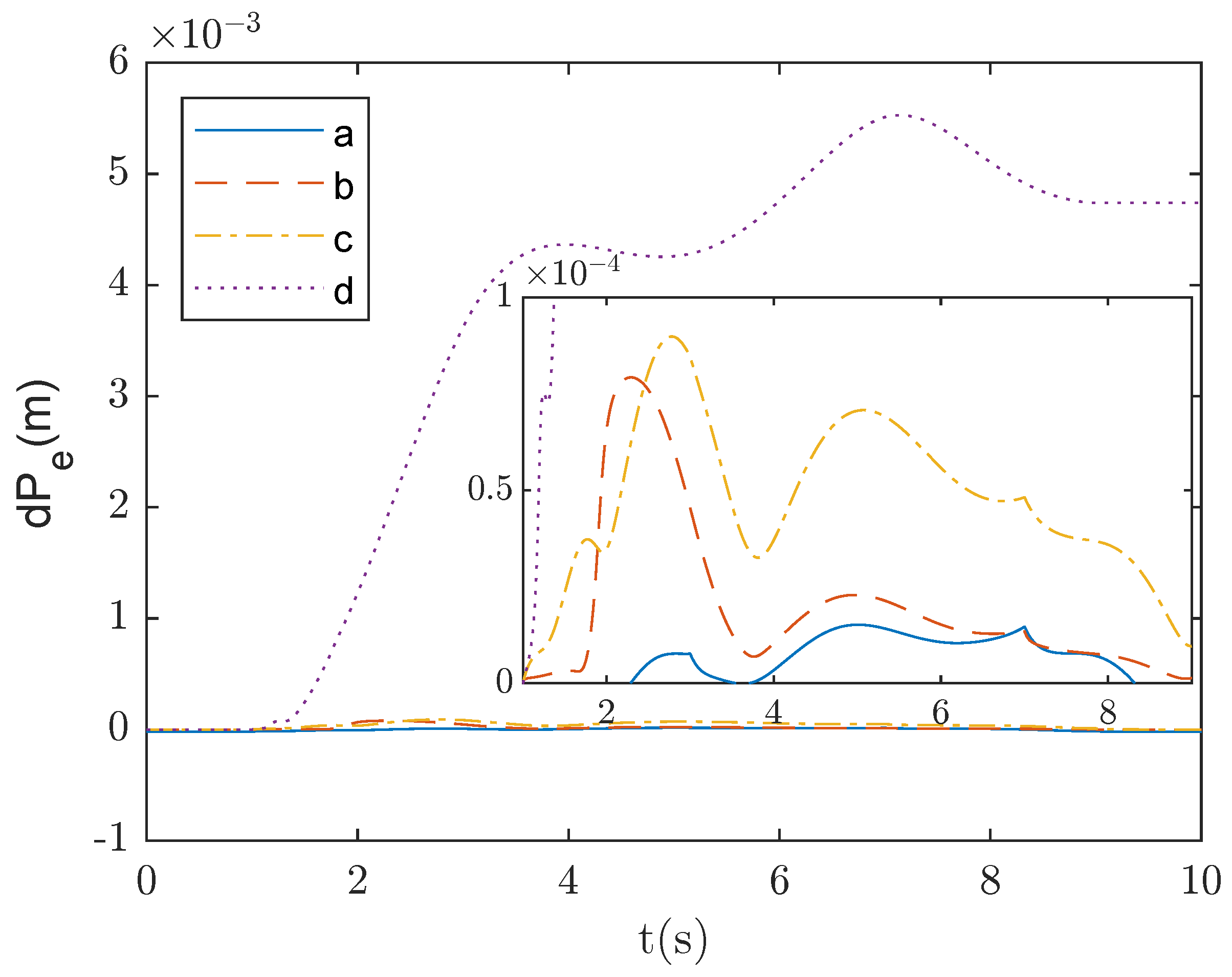
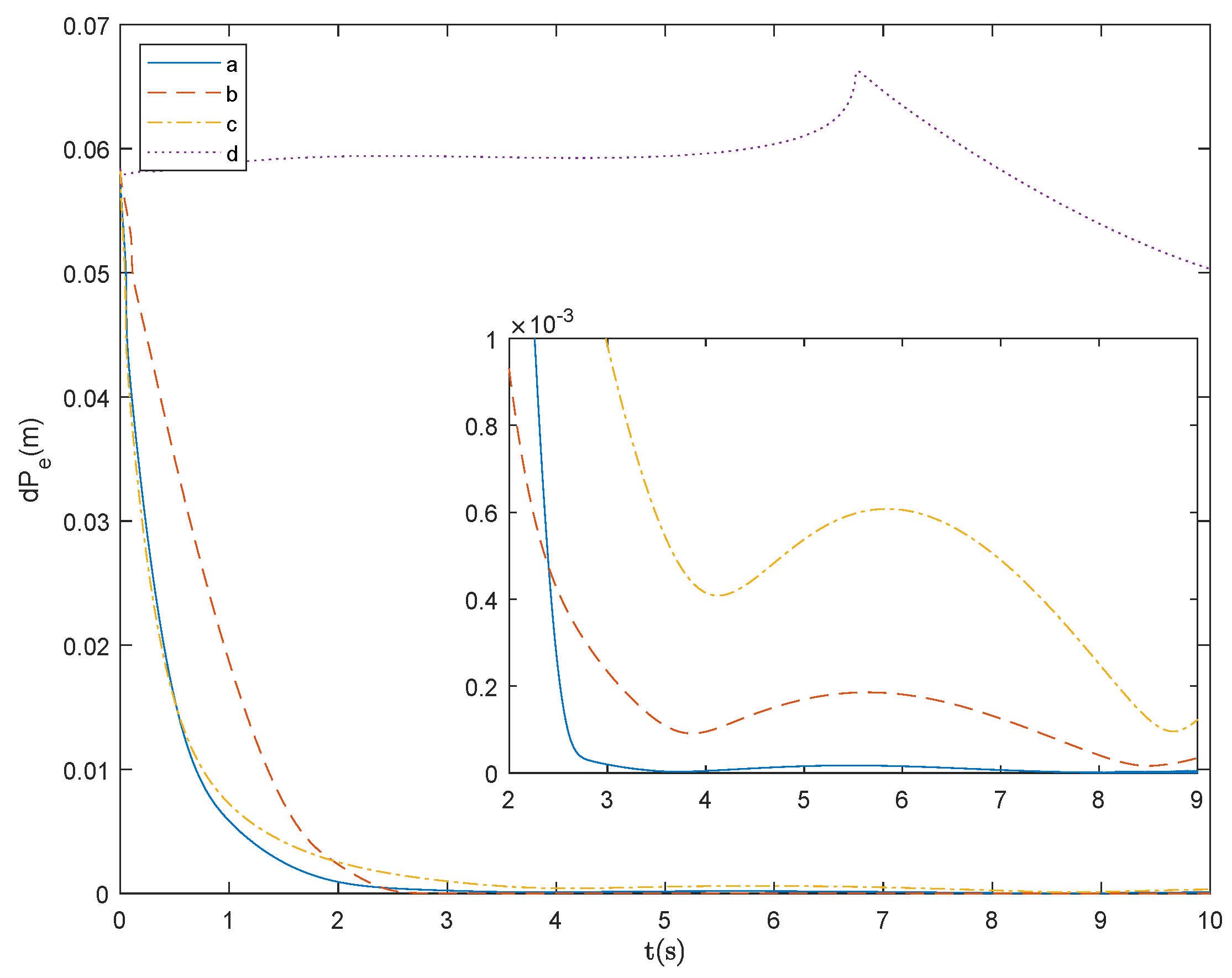
Figure 8 and Figure 9 illustrate the end effector pose errors of the continuum space robot during the trajectory planning process. Line a represents the proposed explicit-time trajectory planning method, line b is based on the finite-time trajectory planning method, line c is based on proportional feedback for trajectory planning, and line d is based solely on the DLS method without pose feedback. From line d, it can be observed that using only singularity avoidance introduces pose errors, and these errors persist after the completion of the trajectory planning task. On the contrary, trajectory planning methods based on pose error feedback, represented by lines a, b, and c, can converge the errors to zero. Line b shows that the finite-time trajectory planning method, although having a smaller overall error, exhibits noticeable singularity issues at 1.7 s, and the errors cannot be quickly eliminated after the trajectory planning task. Line c, representing the widely used proportional feedback method in space robot trajectory planning, shows no apparent singularity or oscillation issues and can effectively eliminate errors after the trajectory planning task. However, the planning accuracy and error convergence speed are lower than line a. Line a demonstrates that the proposed method can keep the trajectory planning error of the robot consistently at a low level and converge to zero at an earlier stage.

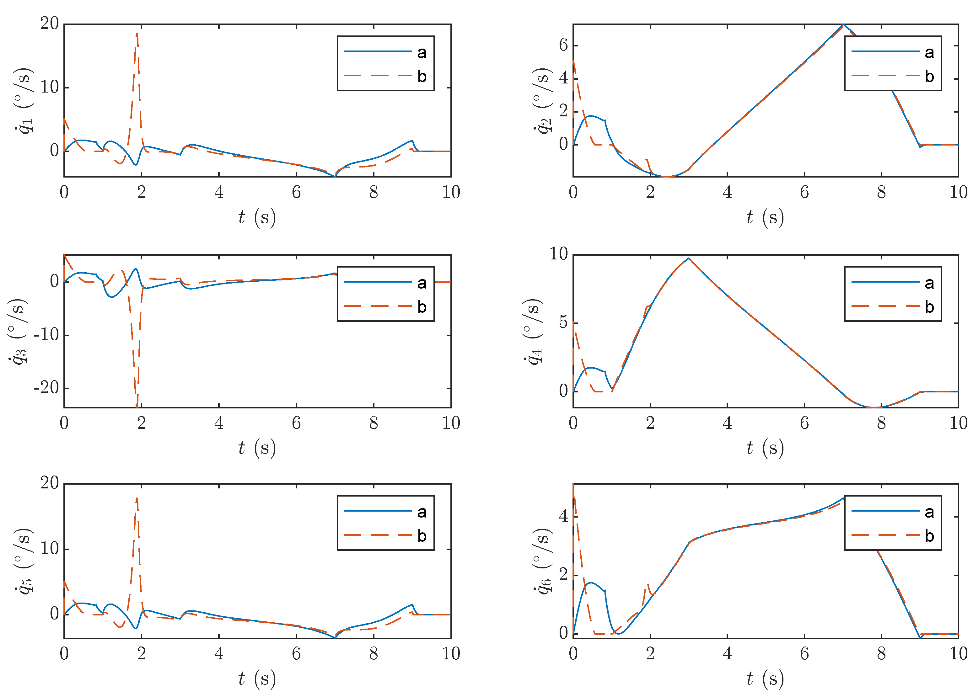
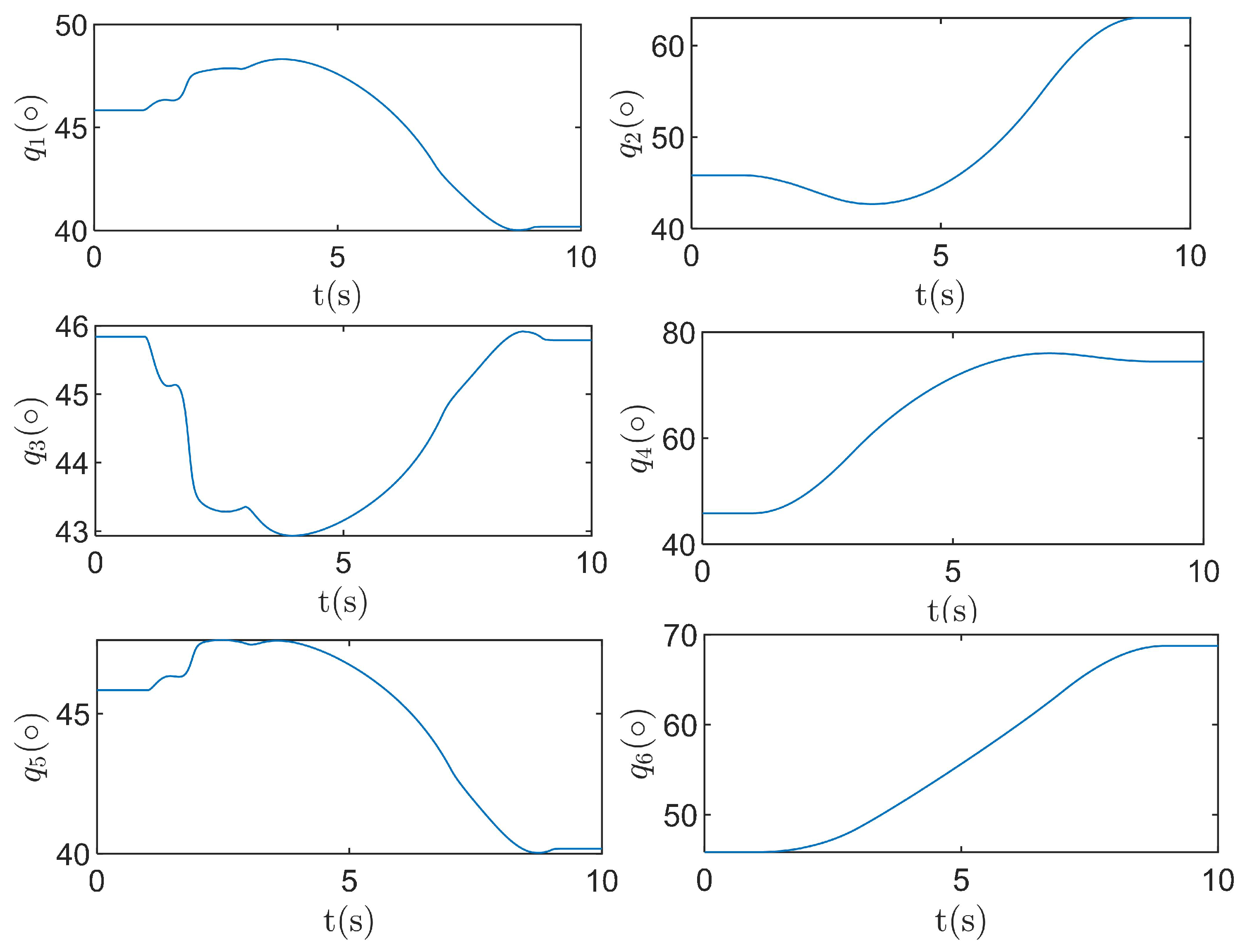
As shown in Figure 10, line a represents the joint velocity planned by the proposed method and line b represents the joint velocity planned by the predefined time method proposed in reference [24]. It can be seen that the joint angular velocity obtained by the proposed trajectory planning method is bounded and continuous, and effectively reduces joint velocity. The joint trajectory obtained using the proposed method is shown in Figure 11.

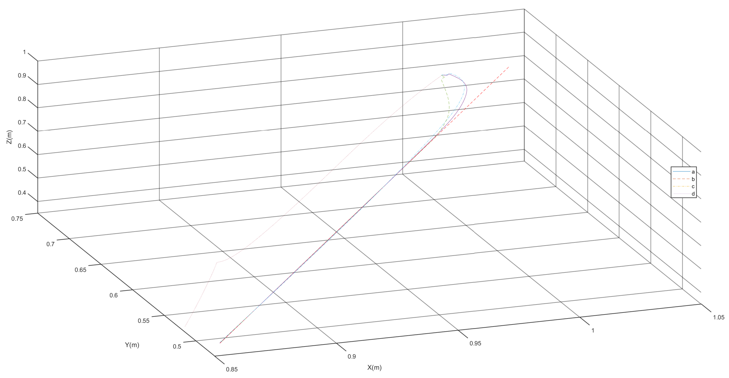
To visually demonstrate the differences in trajectory planning methods, a three-dimensional plot of the end effector’s position trajectory is presented in Figure 12. Considering a scenario where there is a deviation between the initial position of trajectory planning and the expected initial position, with the expected initial joint angles and end effector pose consistent with Table 2, the actual initial position is ${{\mathit{r}}^{\mathbf{\prime }}}_{e0}={\left[1.010.720.83\right]}^{\mathrm{T}}$ (m), the initial orientation is ${\mathit{q}}_{e0}={[0.32-0.700.640.00]}^{\mathrm{T}}$, and the initial joint angles are $\mathit{q}={\left[0.830.830.830.830.830.83\right]}^{\mathrm{T}}$ (rad). Each line in the figure illustrates the convergence of errors. Line d, which does not use pose feedback, fails to eliminate the existing error. Among the trajectory planning methods based on pose feedback, line a, representing the proposed trajectory planning method, demonstrates the fastest convergence and highest accuracy.

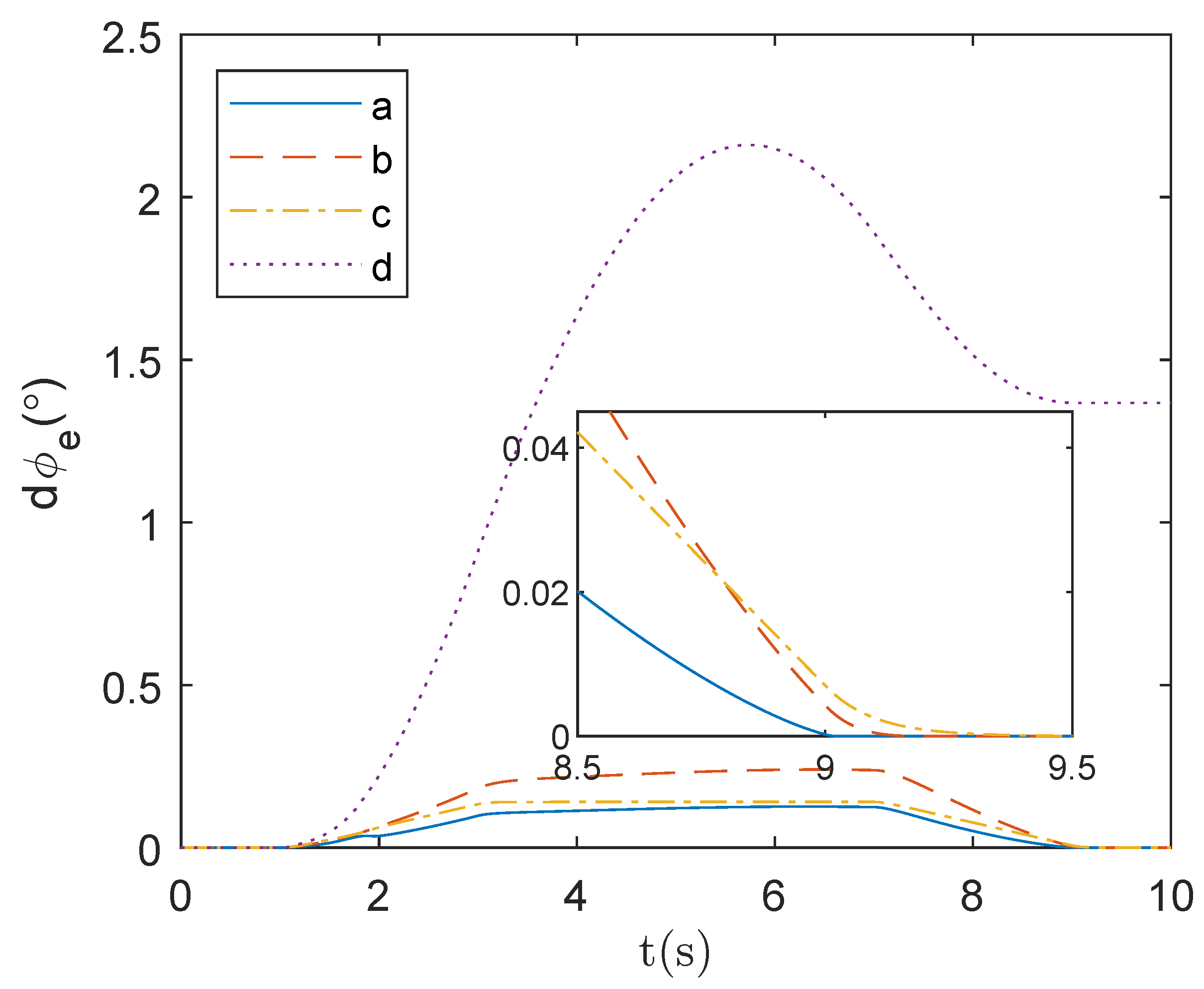
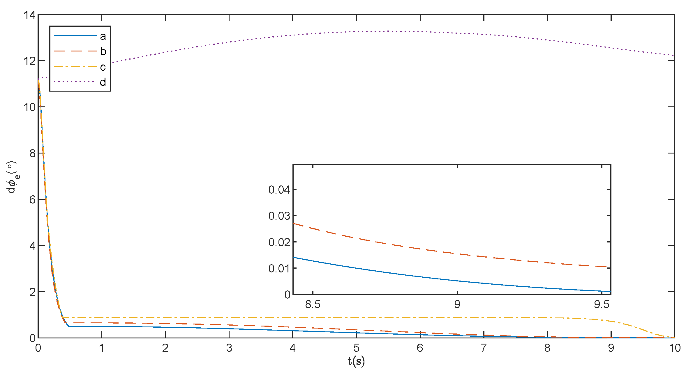
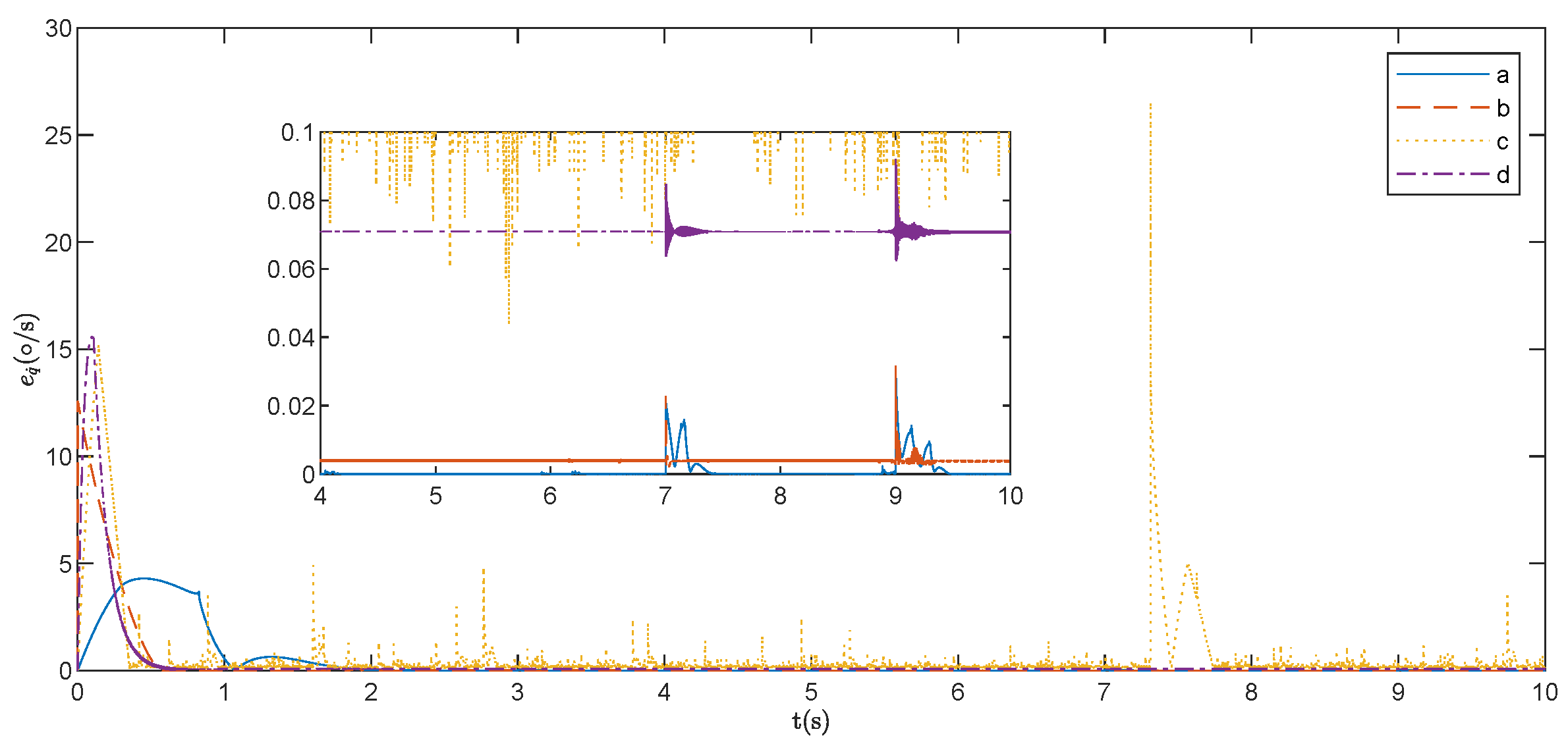
Figure 13 and Figure 14 illustrate the end-effector orientation error of the continuum space robot during the trajectory planning process. From curve d, it is evident that relying solely on a singularity avoidance strategy leads to orientation errors, which persist even after the trajectory planning task is completed. In contrast, trajectory planning methods incorporating orientation error feedback (curves a, b, and c) successfully drive the error to zero. Although curve b (finite-time trajectory planning) exhibits relatively low overall error, it struggles to rapidly eliminate residual errors after completing the trajectory planning task. Curve c (the proportional feedback method, widely used in space robot trajectory planning) does not exhibit significant singularity or oscillation issues and effectively eliminates post-task errors. However, its planning accuracy and error convergence rate are lower than those of curve a. Curve a demonstrates that the proposed method consistently maintains a low trajectory planning error and achieves error convergence to zero at an earlier stage.

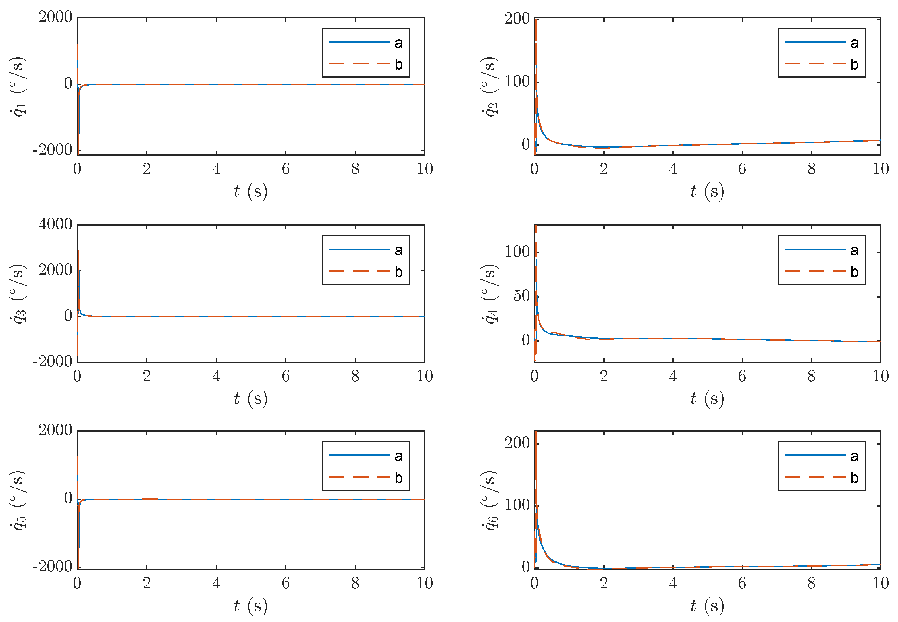
As shown in Figure 15, curve a represents the joint velocity planned by the proposed method, while curve b corresponds to the joint velocity planned using the predefined-time method from [24]. The upper bound of the proposed method in this paper has been marked with a red dashed line. It can be observed that the joint angular velocity obtained through the proposed trajectory planning method is bounded and continuous, effectively reducing joint velocity.

In summary, the trajectory planning method based on explicit time stability theory and pose error feedback can converge errors caused by singular points to zero, enable high-precision tracking of the end effector, and plan appropriate joint angular velocities.

7.2. Simulation and Analysis of Trajectory Tracking

In order to demonstrate the control performance of the explicit-time sliding mode controller proposed in for the continuum space robot, trajectory tracking control simulations were conducted, here considering the bounded uncertainty $\mathit{D}$ of the system $\mathit{D}=20(sint+1\times rand)$. The parameters of the proposed controller are $T_c=2.5$, $m=0.3$, and $e_c=0.05$, $s_c=1$. The convergence time is 5 s.

In the comparative experiments, predefined-time [22], finite-time [27], and conventional asymptotic sliding mode controller were selected for comparison.

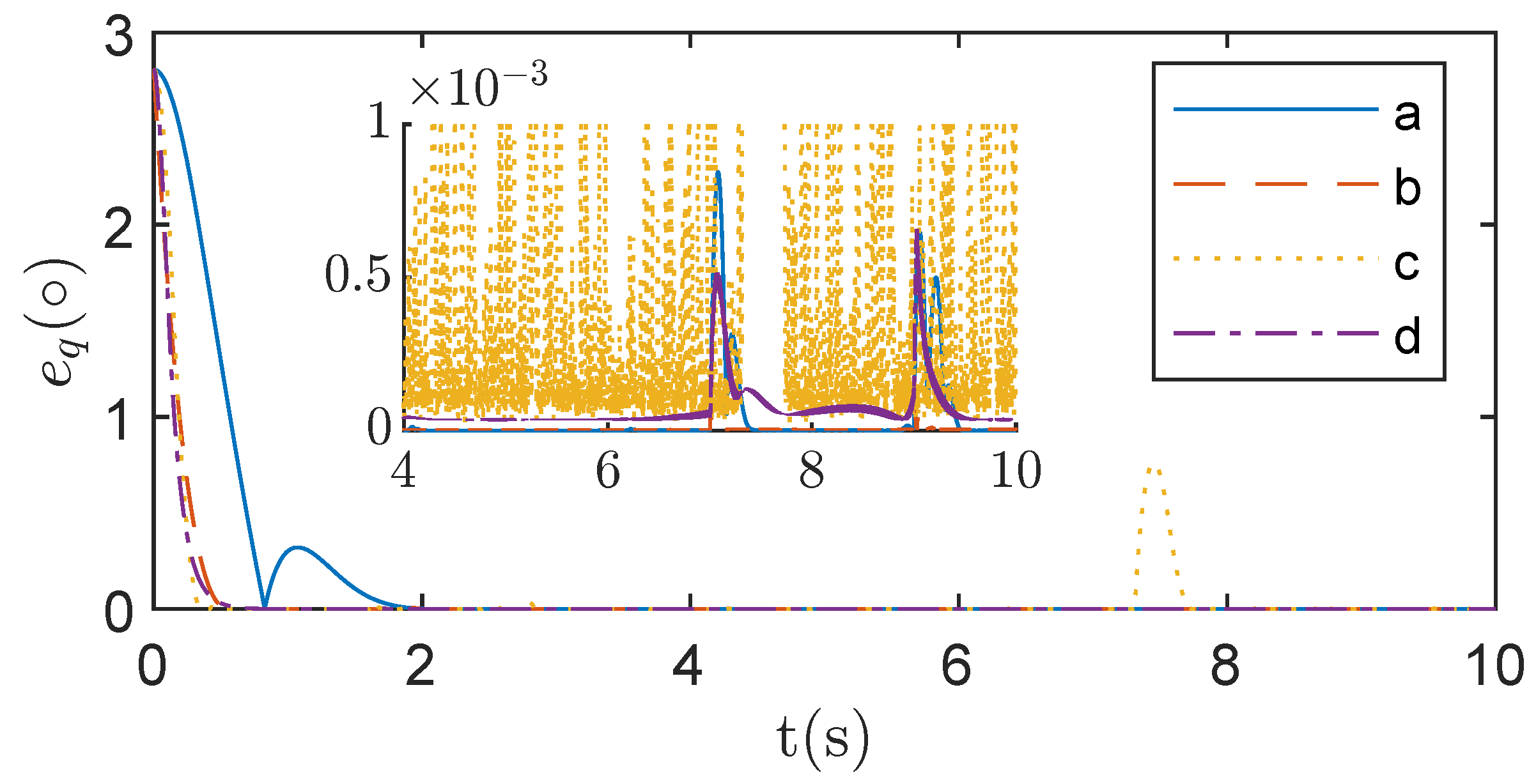
Line a represents the proposed explicit-time controller, line b represents the predefined-time controller, line c represents the finite-time controller, and line d represents the conventional sliding mode controller.

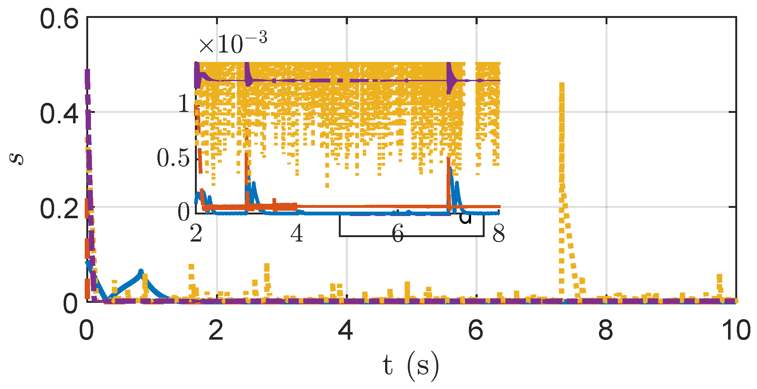
The sliding mode values are depicted in Figure 16. The proposed method facilitates rapid error convergence to zero, and the convergence time is within the explicit upper bound of time. The convergence time of the predefined time is shorter than the method proposed, but the error is higher than the proposed method. The finite-time method demonstrates quick convergence at the beginning but maintains minor oscillations in the later stages. The error of the conventional sliding mode controller is relatively stable, but due to its asymptotic convergence the error is noticeably higher than that of the proposed method. Corresponding control signals are illustrated in Figure 17, and their analysis is similar to the sliding mode analysis, showing that the proposed method yields smaller and smoother control signals.

The stability results of the proposed trajectory tracking control are shown in Figure 18 and Figure 19, with errors converging to zero within the explicit time.

Both the convergence time of the explicit time and the predefined time are less than the ideal convergence time. Although both can ensure convergence time, the explicit time controller can significantly reduce control inputs, thereby decreasing the damage of the controller to the drive mechanism.

In summary, the proposed trajectory tracking control method demonstrates high accuracy and smoother control inputs.

7.3. Simulation and Analysis of Trajectory Planning and Tracking Control

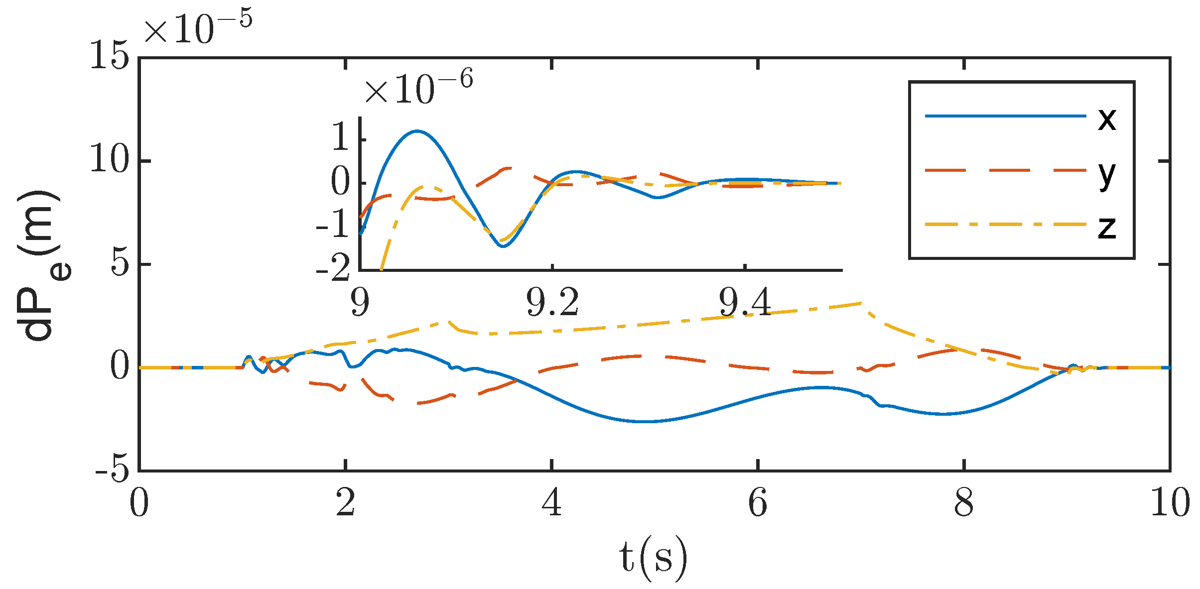
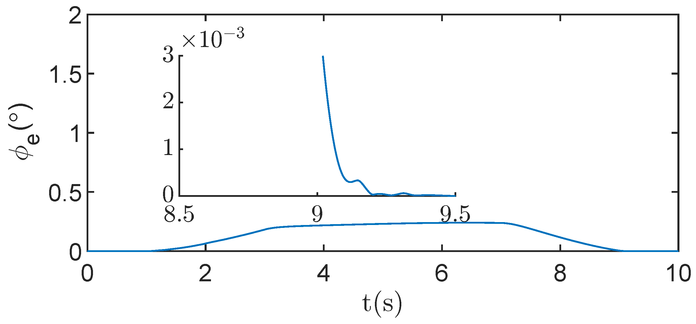
This section presents the co-simulated results of trajectory planning and tracking control for the continuum space robot. As shown in Figure 20 and Figure 21, the pose error of the robot remains consistently at a low level throughout the motion. After leaving the singular region, the accumulated pose error of the robot quickly converges to near zero. Ultimately, the position error converges to below ${10}^{-6}$ m, and the orientation error converges to below ${10}^{-3}$ degrees.

8. Experiment

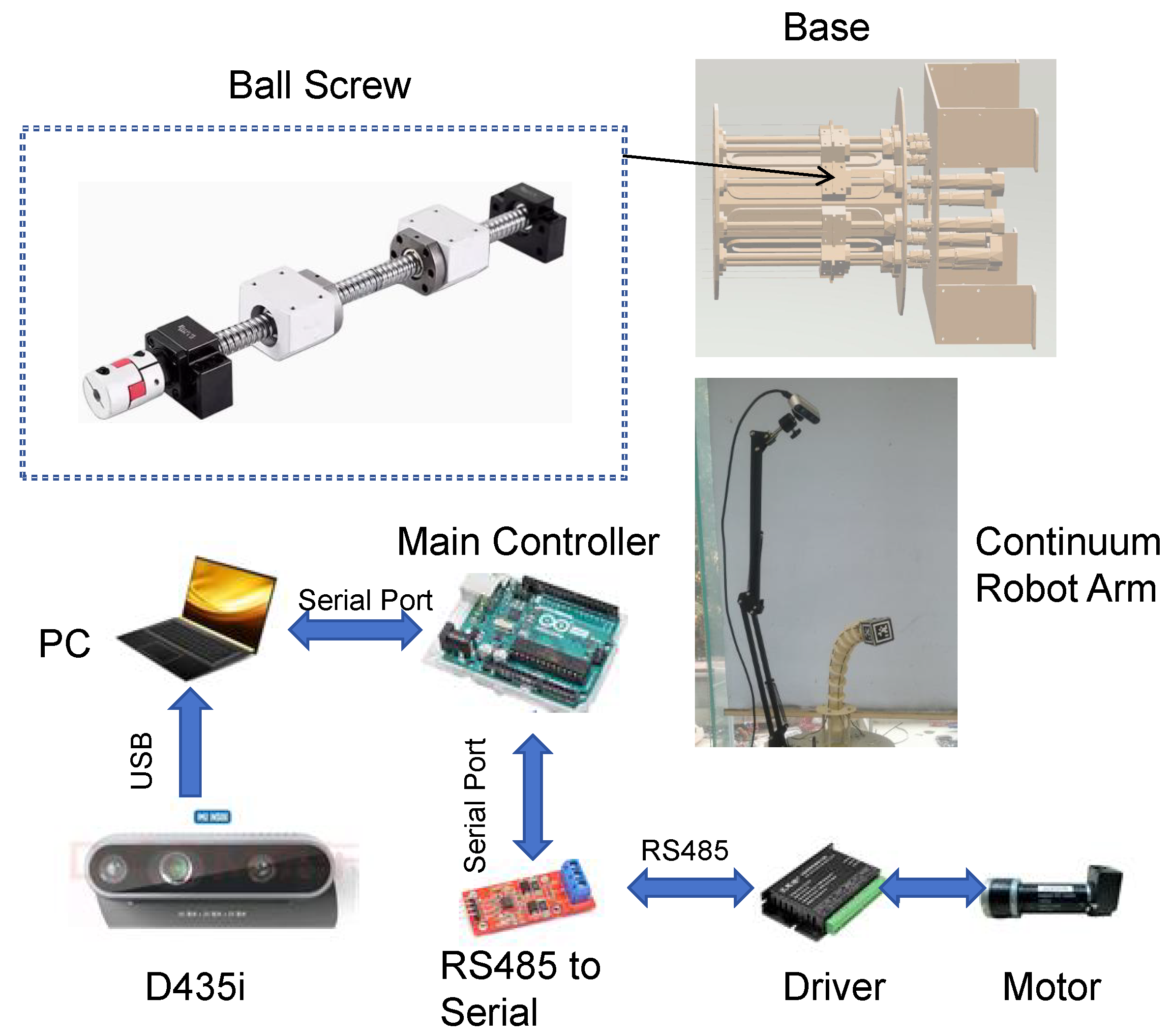
In this paper, a fixed-base, single-segment continuum robot is used to verify the effectiveness of the explicit time algorithm. Figure 22 presents the physical prototype of the continuum robot and its experimental platform. The experimental prototype consists of three main components: the continuum body, the motor control system, and the driving mechanism. The body of the continuum robot is made of a polyurethane (PU) rod synthesized from urethane material. During experiments, the length of the central rod remains fixed, and ten support discs are evenly distributed along the main body to better conform to the constant curvature assumption.The host computer runs MATLAB R2023B, responsible for processing robot motion calculations, trajectory planning, sensor data acquisition, and sending motor control commands. The entire control system operates at a sampling rate of 100 Hz (i.e., executing once every 0.01 s). The core of the motor control system is an Arduino development board, which handles the main control tasks and sends control signals to the AQMD6008NS-TBE driver board (Akelc, Chengdu, Sichuan province, China). This driver board regulates the rotational speed of each motor. The motors used are DC motors from the Maxon Motor brand, equipped with an 84:1 gearbox and a 512-pulse ABZ three-phase encoder. The driving mechanism is designed such that the motors drive the movement of sliders via ball screws, which in turn pull the driving cables to achieve the motion of the continuum robot.

During the experiment, an Intel RealSense D435I depth camera (Intel, Santa Clara, CA, USA) was used to acquire data for obtaining the position information of the continuum robot’s end-effector. The camera has a calibration accuracy of 1 mm. Its position relative to the continuum robot follows an “eye-to-hand” configuration. A cubic marker was attached to the end of the continuum robot. By detecting the April Tag on the marker, the position of the robot arm’s end-effector was obtained. The velocity and acceleration of the end-effector were estimated using a low-pass filter. The acquired data were transmitted to the host computer via a USB interface for processing. During the experiment, the host computer continuously transmitted the processed data to the motor control system in real time. Upon receiving the commands, the control system drove the motors, causing the driving cables on the sliders to move linearly. This adjustment of cable length enabled precise control of the continuum robot’s motion.

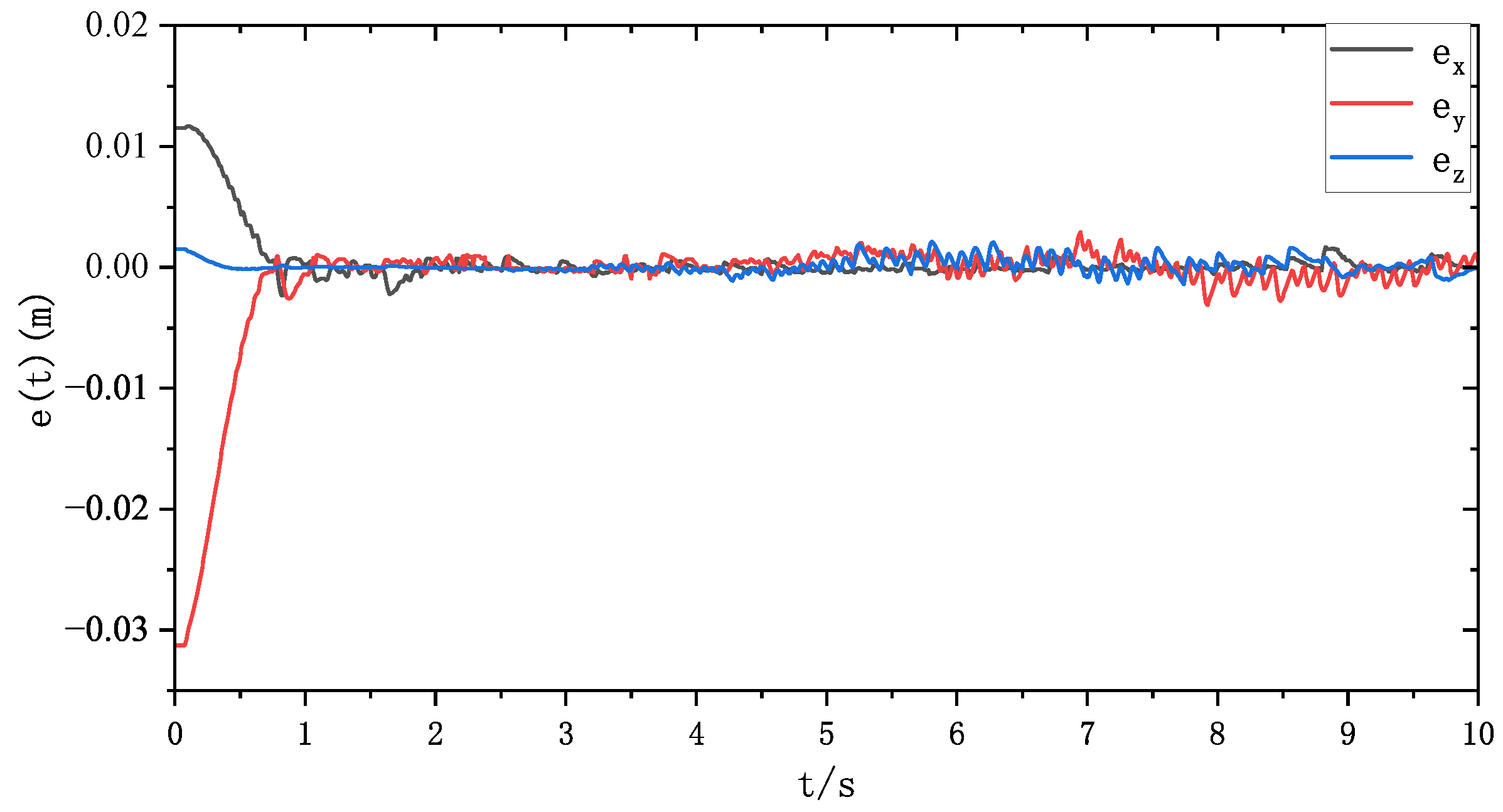
In the experiment, a point-to-point task in 3D space was used for validation. The same planned trajectory as in the simulation was applied, with a duration set to 10 s, as shown in Figure 23. During the experiment, the parameters were set to $T_c=1.5$, $m=0.3$, and $e_c=0.05$. Figure 23 shows the tracking error curve of the actual end-effector position of the continuum robot. It can be seen that the proposed method enables the end-effector position tracking error to converge to near zero within $2T_c$, meeting the predefined convergence time. Figure 24 is a schematic diagram of the continuum robot motion.

9. Conclusions

This paper focuses on the trajectory planning and tracking control issues of continuum space robots based on the explicit time stability. Initially, the kinematic model of the continuum manipulator was derived based on the assumption of PCC. Building upon this, a kinematic model for a free-floating continuum space robot was proposed, integrating pose error feedback. The dynamic model of the underactuated continuum space robot was formulated using the Lagrange method. Subsequently, based on the explicit-time stability theory and singularity avoidance method, a new trajectory planning method was proposed for the free-floating continuum space robot, obtaining smoother joint trajectories. Following this, a corresponding sliding mode controller based on explicit-time stability was proposed to achieve fast and high-precision tracking of joint trajectories with smaller control inputs. Finally, a joint simulation of trajectory planning and tracking control was conducted to reduce errors resulting from singularity avoidance, and high-precision trajectory tracking control for the continuum space robot is realized.

10. Future Recommendation

In future, we should focus on refining the control strategies for continuum space robots by incorporating advanced optimization techniques and machine-learning-based approaches. In particular, reinforcement learning can be explored to develop adaptive control mechanisms that enhance the system’s ability to handle uncertainties and dynamically adjust control parameters in real-time.

Moreover, integrating real-world disturbances, such as space environmental factors and actuator imperfections, into the model will further improve the robustness of trajectory planning and tracking control. Future studies can also investigate the effects of varying payloads and external forces on system performance, optimizing control inputs to ensure stability under different operational conditions.

Additionally, exploring hybrid control strategies that combine explicit-time stability with model predictive control (MPC) or adaptive sliding mode control may enhance the precision and efficiency of trajectory tracking. This approach can help mitigate control input fluctuations while maintaining system stability.

Finally, experimental validation using robotic prototypes in a simulated space environment or under microgravity conditions will be essential to confirm the feasibility and reliability of the proposed methods. By addressing these areas, future research can significantly advance the practical application of continuum space robots in on-orbit servicing, deep-space exploration, and autonomous robotic operations.