
InSAR-RiskLSTM: Enhancing Railway Deformation Risk Prediction with Image-Based Spatial Attention and Temporal LSTM Models


Abstract
1. Introduction
- The proposed model introduces a novel spatial attention mechanism that enhances the model’s focus on critical deformation areas, improving risk detection sensitivity.
- It demonstrates a robust and adaptable framework that is suitable for various railway conditions and spatial environments, providing high efficiency across multiple scenarios.
- The experimental results show that InSAR-RiskLSTM significantly outperforms the baseline models in accuracy and response time, underscoring its effectiveness for real-time risk prediction.
2. Related Work
2.1. InSAR for Infrastructure Deformation Monitoring
2.2. LSTM and Temporal Models in Risk Prediction
2.3. Spatial Attention Mechanisms in Geospatial Applications
3. Methodology
3.1. Overview
| Algorithm 1: InSAR-RiskLSTM: Railway Deformation Risk Prediction |
Input: InSAR imagery data , temporal features , and external factors E. Output: Predicted deformation risk scores . Step 1: Data Preprocessing Extract deformation patterns from InSAR imagery; Normalize and align temporal features ; Integrate external environmental conditions E. Step 2: Spatial Attention Encoding Feed into the Spatial Attention Encoder; Generate attention maps to highlight high-risk regions; Extract spatial feature representations . Step 3: Temporal Risk Prediction Feed into the LSTM-based Temporal Risk Predictor; Model sequential dependencies in deformation time series; Extract temporal feature representations . Step 4: Feature Fusion Combine spatial and temporal features: ; Align multi-source information into a unified representation. Step 5: Risk Score Prediction Generate comprehensive risk scores for railway segments; Assess deformation magnitudes and identify high-risk areas. Step 6: Output and Decision Support Provide risk assessment insights for railway maintenance and mitigation; return Predicted risk scores . |
3.2. Preliminaries
3.3. InSAR-RiskLSTM Framework
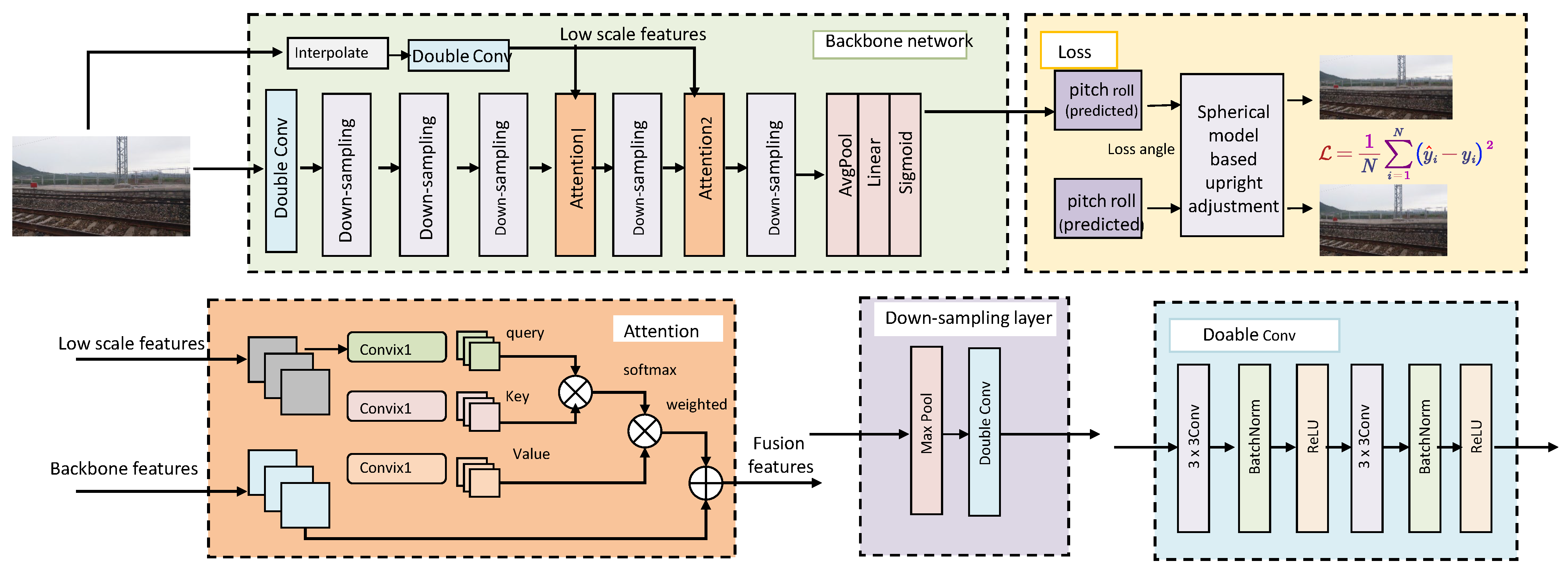
- Spatial Attention Encoder
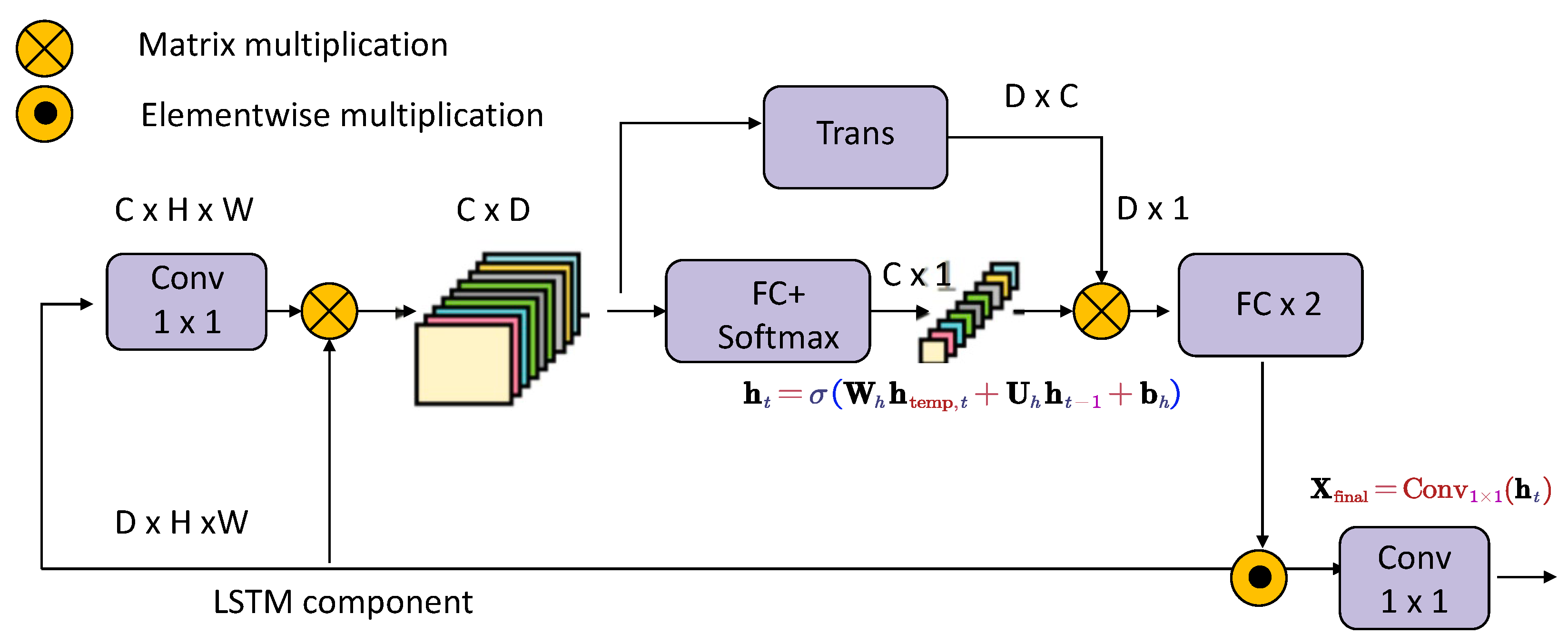
- Temporal Risk Predictor
- Feature Fusion Mechanism
3.4. Spatiotemporal Prior Integration
- Geophysical Dependencies
- Multi-Task Optimization
- Mixture of Experts (MoE) for Adaptive Specialization
4. Experimental Setup
4.1. Dataset
4.2. Experimental Details
| Algorithm 2: Adaptive Multi-Stage Deep Model (AMSDM) Training and Evaluation Algorithm |
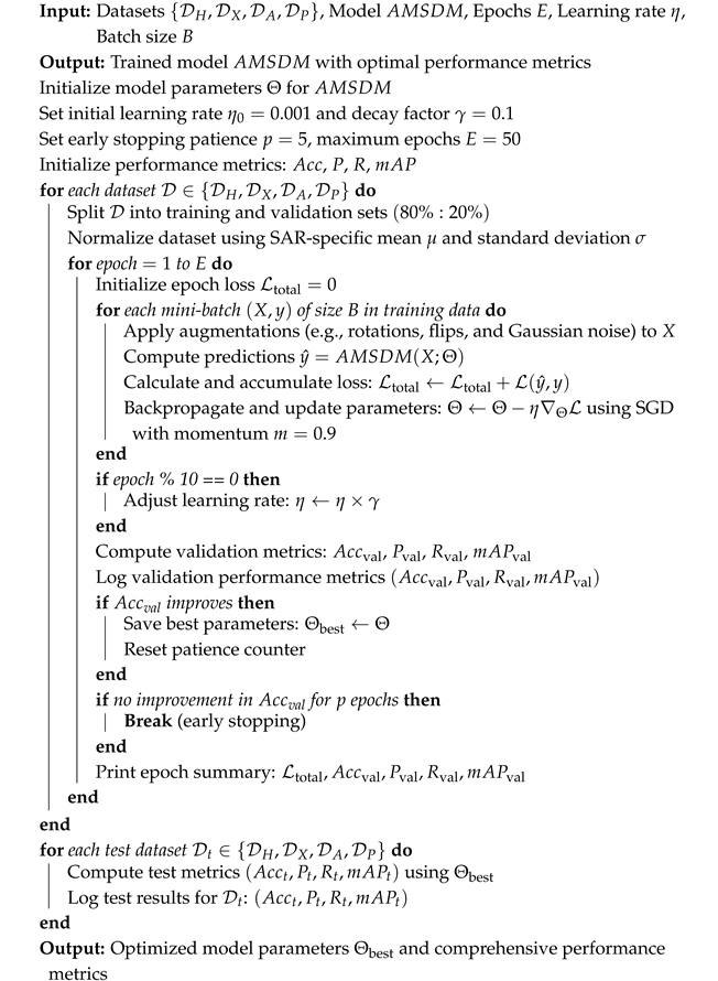 |
4.3. Comparison with SOTA Methods
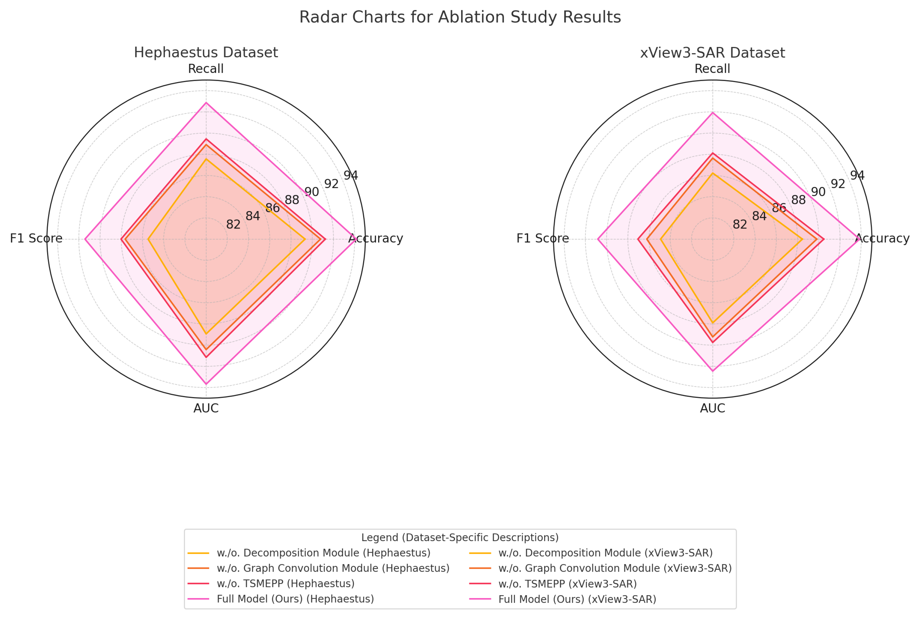
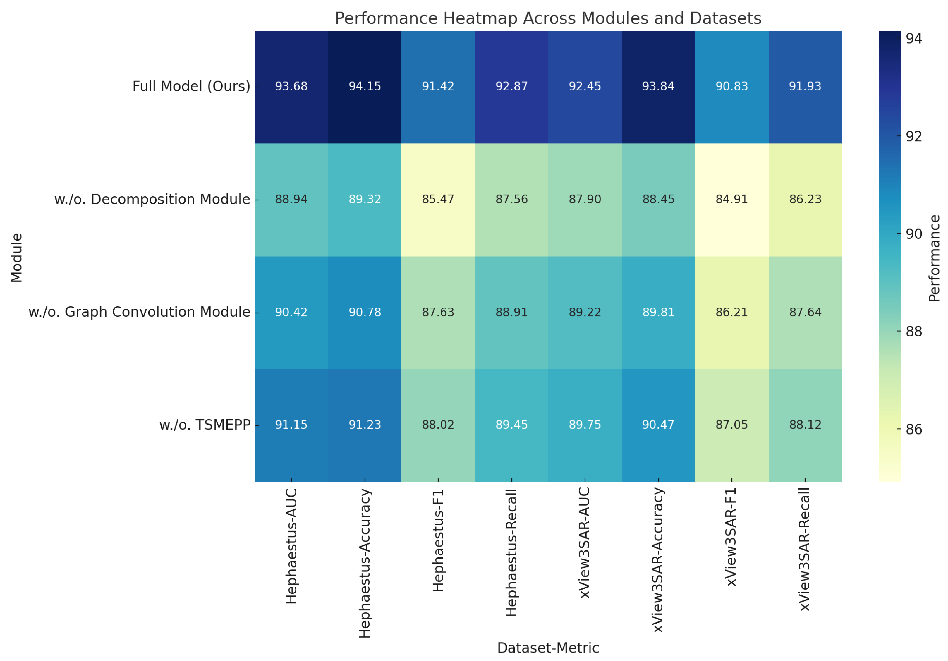
4.4. Ablation Study
5. Discussion
6. Conclusions and Future Work
Author Contributions
Funding
Institutional Review Board Statement
Informed Consent Statement
Data Availability Statement
Conflicts of Interest
References
- Zhang, K.; Yao, Y. Extended UH model and deformation prediction of high-speed railway subgrade. Transp. Geotech. 2023, 39, 100942. [Google Scholar] [CrossRef]
- Yang, J. Study on Large Deformation Prediction and Control Technology of Carbonaceous Slate Tunnel in Lixiang Railway. Geofluids 2022, 2022, 7236065. [Google Scholar] [CrossRef]
- Liu, Y.; Li, P.; Feng, B.; Wang, Z.; Xu, X.; Li, C.; Jing, H. Analysis and Prediction of Railway Infrastructure Deformation Monitoring Data Based on Fractional Order Statistical Theory. IEEE Access 2023, 11, 133428–133439. [Google Scholar] [CrossRef]
- Li, Y.X.; Ma, Y.Y. Research and design of a deformation monitoring system for the platform and canopy of a railway station. J. Phys. Conf. Ser. 2023, 2459, 012101. [Google Scholar]
- Liu, S.; Jiang, W.; Chen, Q.; Wang, J.; Tan, X.; Liu, R.; Ye, Z. Deformation Analysis and Prediction of a High-Speed Railway Suspension Bridge under Multi-Load Coupling. Remote Sens. 2024, 16, 1687. [Google Scholar] [CrossRef]
- Liu, Y.; Zhang, Y.; Su, P.; Zhang, G.; Qiu, P.; Tang, L. Risk Prediction of Rock Bursts and Large Deformations in YL Tunnel of the Chongqing–Kunming High-Speed Railway. Front. Earth Sci. 2022, 10, 892606. [Google Scholar] [CrossRef]
- Qin, Z.; Tao, Z.; Chen, Z.; Zhang, Z.; Tang, C.; Liu, H.; Ren, Q. Deformation Analysis and Prediction of Foundation Pit in Soil-Rock Composite Stratum. Front. Phys. 2022, 9, 817429. [Google Scholar] [CrossRef]
- Jin, X.; Hou, J.; Lee, S.J.; Zhou, D. Recent advances in artificial neural networks and embedded systems for multi-source image fusion. Front. Neurorobotics 2022, 16, 962170. [Google Scholar] [CrossRef] [PubMed]
- Lyu, B.; Liu, B.; Xie, B.; Xiao, H.; Liu, X.; Zhang, Z.; Li, Y.; Huang, X.; Shi, F. Study on InSAR deformation information extraction and stress state assessment in a railway tunnel in a plateau area. Front. Earth Sci. 2024, 12, 1367978. [Google Scholar] [CrossRef]
- Liang, B.; Wei, G. Ediction of railway settlement deformation based on improved GM-AR model. J. Phys. Conf. Ser. 2021, 2044, 012154. [Google Scholar] [CrossRef]
- Yan, H.; Zhao, X.; Jian, L.; Long, R.; Xiao, D.; Chen, M. Subgrade uplift prediction along a high-speed railway using machine learning techniques in Sichuan, China. Front. Earth Sci. 2024, 12, 1403965. [Google Scholar] [CrossRef]
- Abiodun, L.E.; Salim, N.A.M. Numerical Analysis for Prediction of Optimum Deformation of Long Tunnel Crown Stability with Respect to Excavation Depth. Educatum J. Sci. Math. Technol. 2022, 9, 79–91. [Google Scholar] [CrossRef]
- Wang, G. RL-CWtrans Net: Multimodal swimming coaching driven via robot vision. Front. Neurorobotics 2024, 18, 1439188. [Google Scholar] [CrossRef] [PubMed]
- Zhang, Y. Prediction model of surrounding rock deformation in double-continuous-arch tunnel based on the ABC-WNN. Railw. Sci. 2024, 3, 717–730. [Google Scholar] [CrossRef]
- Qiu, D.; Liu, Y.; Xue, Y.; Su, M.; Zhao, Y.; Cui, J.; Kong, F.; Li, Z. Prediction of the Surrounding Rock Deformation Grade for a High-Speed Railway Tunnel Based on Rough Set Theory and a Cloud Model. Iran. J. Sci. Technol. Trans. Civ. Eng. 2021, 45, 303–314. [Google Scholar] [CrossRef]
- Li, S.; Li, Y.; Xu, L. Deformation Pattern and Failure Mechanism of Railway Embankment Caused by Lake Water Fluctuation Using Earth Observation and On-Site Monitoring Techniques. Water 2023, 15, 4284. [Google Scholar] [CrossRef]
- Yin, Y.; Wei, C.; Wang, H.; Wang, Z.; Deng, Q. Prediction of thawing settlement coefficient of frozen soil using 5G communication. Soft Comput. 2022, 26, 10837–10852. [Google Scholar] [CrossRef]
- Mei, H.; Satvati, S.; Leng, W. Experimental study on permanent deformation characteristics of coarse-grained soil under repeated dynamic loading. Railw. Eng. Sci. 2021, 29, 94–107. [Google Scholar] [CrossRef]
- Ramadan, A.; Jing, P.; Zhang, J.; Zohny, H.N. Numerical Analysis of Additional Stresses in Railway Track Elements Due to Subgrade Settlement Using FEM Simulation. Appl. Sci. 2021, 11, 8501. [Google Scholar] [CrossRef]
- Li, Q.; Huang, X.; Chen, H.; He, F.; Chen, Q.; Wang, Z. Advancing Micro-Action Recognition with Multi-Auxiliary Heads and Hybrid Loss Optimization. In Proceedings of the 32nd ACM International Conference on Multimedia, Melbourne, Australia, 28 October–1 November 2024; pp. 11313–11319. [Google Scholar]
- Jin, X.; Wu, N.; Jiang, Q.; Kou, Y.; Duan, H.; Wang, P.; Yao, S. A dual descriptor combined with frequency domain reconstruction learning for face forgery detection in deepfake videos. Forensic Sci. Int. Digit. Investig. 2024, 49, 301747. [Google Scholar] [CrossRef]
- Ruiying, P. Multimodal Fusion-powered English Speaking Robot. Front. Neurorobot. 2024, 18, 1478181. [Google Scholar]
- Li, Z.; Peng, Y.; Li, J.; Tang, Z. Composite Foundation Settlement Prediction Based on LSTM–Transformer Model for CFG. Appl. Sci. 2024, 14, 732. [Google Scholar] [CrossRef]
- Bernal, E.; Spiryagin, M.; Vollebregt, E.; Oldknow, K.; Stichel, S.; Shrestha, S.; Ahmad, S.; Wu, Q.; Sun, Y.; Cole, C. Prediction of rail surface damage in locomotive traction operations using laboratory-field measured and calibrated data. Eng. Fail. Anal. 2022, 135, 106165. [Google Scholar] [CrossRef]
- Coelho, B.Z.; Varandas, J.N.; Hijma, M.P.; Zoeteman, A. Towards network assessment of permanent railway track deformation. Transp. Geotech. 2021, 29, 100578. [Google Scholar] [CrossRef]
- Ansari, A.; Rao, K.S.; Jain, A.K. Application of microzonation towards system-wide seismic risk assessment of railway network. Transp. Infrastruct. Geotechnol. 2024, 11, 1119–1142. [Google Scholar] [CrossRef]
- Wang, J.; Yang, Y.; Tan, Z.; Li, D.; Liu, Q. Correction of Point Load Strength on Irregular Carbonaceous Slate in the Luang Prabang Suture Zone and the Prediction of Uniaxial Compressive Strength. Appl. Sci. 2022, 12, 9147. [Google Scholar] [CrossRef]
- Pillai, N.; Shih, J.; Roberts, C. Evaluation of Numerical Simulation Approaches for Simulating Train–Track Interactions and Predicting Rail Damage in Railway Switches and Crossings (SCs). Infrastructures 2021, 6, 63. [Google Scholar] [CrossRef]
- Xue, Y.A.; Zou, Y.F.; Li, H.Y.; Zhang, W.Z. Regional subsidence monitoring and prediction along high-speed railways based on PS-InSAR and LSTM. Sci. Rep. 2024, 14, 24622. [Google Scholar] [CrossRef] [PubMed]
- Fan, R.; Chen, T.; Wang, S.; Jiang, H.; Yin, X. Study on Influencing Factors and Prediction of Tunnel Floor Heave in Gently Inclined Thin-Layered Rock Mass. Appl. Sci. 2024, 14, 7701. [Google Scholar] [CrossRef]
- Jin, X.; Liu, L.; Ren, X.; Jiang, Q.; Lee, S.J.; Zhang, J.; Yao, S. A restoration scheme for spatial and spectral resolution of panchromatic image using convolutional neural network. IEEE J. Sel. Top. Appl. Earth Obs. Remote. Sens. 2024, 3379–3393. [Google Scholar] [CrossRef]
- Chen, L.; Chen, J.; Wang, C.; Dai, Y.; Guo, R.; Huang, Q. Modeling of Moisture Content of Subgrade Materials in High-Speed Railway Using a Deep Learning Method. Adv. Mater. Sci. Eng. 2021, 2021, 6166489. [Google Scholar] [CrossRef]
- Gao, Y.; Schreiber, P.; Wilk, S.; Hanson, A.C.; Li, T.; Li, D. Update and Case Studies of Geotrack™: A Software for Railway Track and Subgrade Analysis. In Lecture Notes in Civil Engineering; Springer International Publishing: Cham, Switzerland, 2021. [Google Scholar]
- Punetha, P.; Nimbalkar, S. Mathematical Modeling of the Short-Term Performance of Railway Track Under Train-Induced Loading. In Lecture Notes in Civil Engineering; Springer International Publishing: Cham, Switzerland, 2021. [Google Scholar]
- Gomes, V.; Eck, S.; de Jesus, A.D. Cyclic Hardening and Fatigue Damage Features of 51CrV4 Steel for the Crossing Nose Design. Appl. Sci. 2023, 13, 8308. [Google Scholar] [CrossRef]
- Jin, X.; Zhang, P.; He, Y.; Jiang, Q.; Wang, P.; Hou, J.; Zhou, W.; Yao, S. A theoretical analysis of continuous firing condition for pulse-coupled neural networks with its applications. Eng. Appl. Artif. Intell. 2023, 126, 107101. [Google Scholar] [CrossRef]
- Connor, A.; Harris, A.; Cooper, N.; Poshyvanyk, D. Can we automatically fix bugs by learning edit operations? In Proceedings of the 2022 IEEE International Conference on Software Analysis, Evolution and Reengineering (SANER), Honolulu, HI, USA, 15–18 March 2022; pp. 782–792. [Google Scholar]
- Cao, T.T.; Luckett, C.; Williams, J.; Cooke, T.; Yip, B.; Rajagopalan, A.; Wong, S. Sarfish: Space-based maritime surveillance using complex synthetic aperture radar imagery. In Proceedings of the 2022 International Conference on Digital Image Computing: Techniques and Applications (DICTA), Sydney, Australia, 30 November–2 December 2022; pp. 1–8. [Google Scholar]
- Vásquez-Salazar, R.D.; Cardona-Mesa, A.A.; Gómez, L.; Travieso-González, C.M.; Garavito-González, A.F.; Vásquez-Cano, E. Labeled dataset for training despeckling filters for SAR imagery. Data Brief 2024, 53, 110065. [Google Scholar] [CrossRef]
- Xu, W.; Yuan, X.; Hu, Q.; Li, J. SAR-optical feature matching: A large-scale patch dataset and a deep local descriptor. Int. J. Appl. Earth Obs. Geoinf. 2023, 122, 103433. [Google Scholar] [CrossRef]
- Cahuantzi, R.; Chen, X.; Güttel, S. A comparison of LSTM and GRU networks for learning symbolic sequences. In Proceedings of the Science and Information Conference, London, UK, 27–31 October 2023; Springer: Berlin/Heidelberg, Germany, 2023; pp. 771–785. [Google Scholar]
- Han, K.; Wang, Y.; Chen, H.; Chen, X.; Guo, J.; Liu, Z.; Tang, Y.; Xiao, A.; Xu, C.; Xu, Y.; et al. A survey on vision transformer. IEEE Trans. Pattern Anal. Mach. Intell. 2022, 45, 87–110. [Google Scholar] [CrossRef] [PubMed]
- Fan, J.; Zhang, K.; Huang, Y.; Zhu, Y.; Chen, B. Parallel spatio-temporal attention-based TCN for multivariate time series prediction. Neural Comput. Appl. 2023, 35, 13109–13118. [Google Scholar] [CrossRef]
- Ismail Fawaz, H.; Lucas, B.; Forestier, G.; Pelletier, C.; Schmidt, D.F.; Weber, J.; Webb, G.I.; Idoumghar, L.; Muller, P.A.; Petitjean, F. Inceptiontime: Finding alexnet for time series classification. Data Min. Knowl. Discov. 2020, 34, 1936–1962. [Google Scholar] [CrossRef]
- Koonce, B.; Koonce, B. ResNet 50. In Convolutional Neural Networks with Swift for Tensorflow: Image Recognition and Dataset Categorization; Apress: Berkeley, CA, USA, 2021; pp. 63–72. [Google Scholar]


| Model | Hephaestus Dataset | xView3-SAR Dataset | ||||||
|---|---|---|---|---|---|---|---|---|
| Accuracy | Recall | F1-Score | AUC | Accuracy | Recall | F1-Score | AUC | |
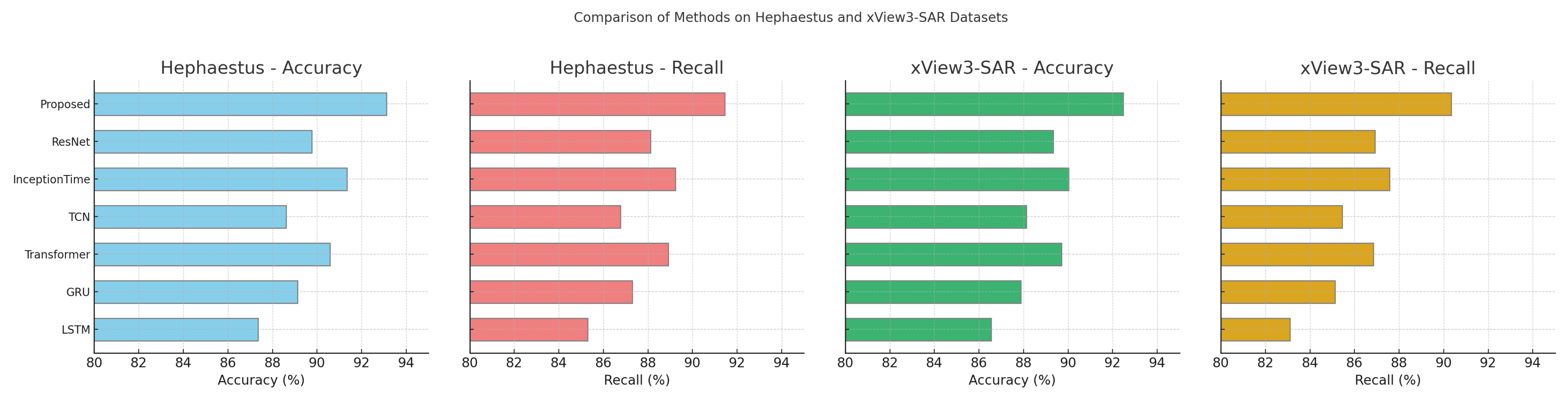
| LSTM [40] | 87.35 ± 0.03 | 85.29 ± 0.02 | 83.47 ± 0.02 | 88.92 ± 0.03 | 86.54 ± 0.02 | 83.10 ± 0.02 | 82.24 ± 0.02 | 87.63 ± 0.03 |
| GRU [41] | 89.12 ± 0.02 | 87.30 ± 0.02 | 86.19 ± 0.02 | 89.45 ± 0.03 | 87.88 ± 0.03 | 85.12 ± 0.02 | 83.75 ± 0.02 | 88.15 ± 0.02 |
| Transformer [42] | 90.58 ± 0.03 | 88.91 ± 0.02 | 87.43 ± 0.02 | 90.31 ± 0.03 | 89.71 ± 0.03 | 86.84 ± 0.02 | 85.64 ± 0.02 | 89.42 ± 0.03 |
| TCN [43] | 88.62 ± 0.02 | 86.77 ± 0.02 | 85.39 ± 0.02 | 88.74 ± 0.03 | 88.12 ± 0.02 | 85.45 ± 0.02 | 84.29 ± 0.02 | 88.10 ± 0.03 |
| InceptionTime [44] | 91.34 ± 0.03 | 89.23 ± 0.02 | 88.47 ± 0.02 | 90.82 ± 0.03 | 90.03 ± 0.03 | 87.58 ± 0.02 | 86.31 ± 0.02 | 89.75 ± 0.02 |
| ResNet [45] | 89.77 ± 0.02 | 88.12 ± 0.02 | 86.85 ± 0.02 | 89.33 ± 0.03 | 89.34 ± 0.02 | 86.91 ± 0.02 | 85.62 ± 0.02 | 89.02 ± 0.03 |
| Ours (Proposed Model) | 93.12 ± 0.02 | 91.45 ± 0.02 | 90.17 ± 0.02 | 92.63 ± 0.03 | 92.48 ± 0.03 | 90.34 ± 0.02 | 89.02 ± 0.02 | 91.27 ± 0.02 |
| Model | ASF SAR Dataset | SAR Patch Dataset | ||||||
|---|---|---|---|---|---|---|---|---|
| Accuracy | Recall | F1-Score | AUC | Accuracy | Recall | F1-Score | AUC | |
| LSTM [40] | 88.27 ± 0.03 | 86.14 ± 0.02 | 84.39 ± 0.02 | 89.32 ± 0.03 | 87.42 ± 0.02 | 84.52 ± 0.02 | 83.58 ± 0.02 | 88.21 ± 0.03 |
| GRU [41] | 89.91 ± 0.02 | 88.05 ± 0.02 | 86.62 ± 0.02 | 90.17 ± 0.03 | 88.73 ± 0.03 | 85.89 ± 0.02 | 84.74 ± 0.02 | 89.56 ± 0.02 |
| Transformer [42] | 91.47 ± 0.03 | 89.78 ± 0.02 | 88.23 ± 0.02 | 91.05 ± 0.03 | 90.24 ± 0.03 | 87.12 ± 0.02 | 86.02 ± 0.02 | 90.43 ± 0.03 |
| TCN [43] | 89.83 ± 0.02 | 87.24 ± 0.02 | 85.82 ± 0.02 | 89.92 ± 0.03 | 89.17 ± 0.02 | 86.53 ± 0.02 | 85.29 ± 0.02 | 89.14 ± 0.03 |
| InceptionTime [44] | 92.18 ± 0.03 | 90.34 ± 0.02 | 89.07 ± 0.02 | 91.68 ± 0.03 | 90.97 ± 0.03 | 88.24 ± 0.02 | 87.02 ± 0.02 | 90.85 ± 0.02 |
| ResNet [45] | 90.35 ± 0.02 | 88.56 ± 0.02 | 87.19 ± 0.02 | 90.12 ± 0.03 | 89.87 ± 0.02 | 87.21 ± 0.02 | 86.04 ± 0.02 | 89.76 ± 0.03 |
| Ours (Proposed Model) | 94.03 ± 0.02 | 92.47 ± 0.02 | 91.18 ± 0.02 | 93.52 ± 0.03 | 93.67 ± 0.03 | 91.43 ± 0.02 | 90.05 ± 0.02 | 92.14 ± 0.02 |
| Model | Hephaestus Dataset | xView3-SAR Dataset | ||||||
|---|---|---|---|---|---|---|---|---|
| Accuracy | Recall | F1-Score | AUC | Accuracy | Recall | F1-Score | AUC | |
| w./o. Decomposition Module | 89.32 ± 0.02 | 87.56 ± 0.02 | 85.47 ± 0.02 | 88.94 ± 0.03 | 88.45 ± 0.02 | 86.23 ± 0.02 | 84.91 ± 0.02 | 87.90 ± 0.03 |
| w./o. Graph Convolution Module | 90.78 ± 0.03 | 88.91 ± 0.02 | 87.63 ± 0.02 | 90.42 ± 0.03 | 89.81 ± 0.03 | 87.64 ± 0.02 | 86.21 ± 0.02 | 89.22 ± 0.03 |
| w./o. TSMEPP | 91.23 ± 0.02 | 89.45 ± 0.02 | 88.02 ± 0.02 | 91.15 ± 0.03 | 90.47 ± 0.02 | 88.12 ± 0.02 | 87.05 ± 0.02 | 89.75 ± 0.03 |
| Full Model (Ours) | 94.15 ± 0.02 | 92.87 ± 0.02 | 91.42 ± 0.02 | 93.68 ± 0.03 | 93.84 ± 0.03 | 91.93 ± 0.02 | 90.83 ± 0.02 | 92.45 ± 0.02 |
| Model | ASF SAR Dataset | SAR Patch Dataset | ||||||
|---|---|---|---|---|---|---|---|---|
| Accuracy | Recall | F1-Score | AUC | Accuracy | Recall | F1-Score | AUC | |
| w./o. Decomposition Module | 90.28 ± 0.02 | 88.14 ± 0.02 | 86.53 ± 0.02 | 89.72 ± 0.03 | 89.45 ± 0.02 | 87.23 ± 0.02 | 85.91 ± 0.02 | 88.34 ± 0.03 |
| w./o. Graph Convolution Module | 91.67 ± 0.03 | 89.55 ± 0.02 | 88.02 ± 0.02 | 90.84 ± 0.03 | 90.31 ± 0.03 | 88.14 ± 0.02 | 86.87 ± 0.02 | 89.56 ± 0.03 |
| w./o. TSMEPP | 92.13 ± 0.02 | 90.23 ± 0.02 | 88.67 ± 0.02 | 91.47 ± 0.03 | 91.12 ± 0.02 | 89.02 ± 0.02 | 87.63 ± 0.02 | 90.35 ± 0.03 |
| Full Model (Ours) | 94.87 ± 0.02 | 93.12 ± 0.02 | 91.45 ± 0.02 | 93.98 ± 0.03 | 93.56 ± 0.03 | 91.75 ± 0.02 | 90.53 ± 0.02 | 92.87 ± 0.02 |
| Scenario | Accuracy (%) | Recall (%) | F1-Score (%) | Robustness Index |
|---|---|---|---|---|
| Flat Terrain | 93.8 ± 0.4 | 91.5 ± 0.5 | 92.1 ± 0.4 | 1.00 |
| Mountainous Terrain | 92.4 ± 0.6 | 90.2 ± 0.7 | 90.8 ± 0.6 | 0.98 |
| Urban Railway | 91.1 ± 0.5 | 89.0 ± 0.6 | 89.5 ± 0.5 | 0.97 |
| Rainy Condition | 90.5 ± 0.7 | 88.2 ± 0.8 | 88.7 ± 0.7 | 0.96 |
| Snowy Condition | 89.9 ± 0.8 | 87.6 ± 0.9 | 88.0 ± 0.8 | 0.95 |
| Dry Condition | 93.5 ± 0.5 | 91.2 ± 0.6 | 91.7 ± 0.5 | 1.00 |
| Average | 91.9 | 89.6 | 90.1 | 0.98 |
Disclaimer/Publisher’s Note: The statements, opinions and data contained in all publications are solely those of the individual author(s) and contributor(s) and not of MDPI and/or the editor(s). MDPI and/or the editor(s) disclaim responsibility for any injury to people or property resulting from any ideas, methods, instructions or products referred to in the content. |
© 2025 by the authors. Licensee MDPI, Basel, Switzerland. This article is an open access article distributed under the terms and conditions of the Creative Commons Attribution (CC BY) license (https://creativecommons.org/licenses/by/4.0/).
Share and Cite
Lyu, B.; Zhang, Z.; Fill, H.D. InSAR-RiskLSTM: Enhancing Railway Deformation Risk Prediction with Image-Based Spatial Attention and Temporal LSTM Models. Appl. Sci. 2025, 15, 2371. https://doi.org/10.3390/app15052371
Lyu B, Zhang Z, Fill HD. InSAR-RiskLSTM: Enhancing Railway Deformation Risk Prediction with Image-Based Spatial Attention and Temporal LSTM Models. Applied Sciences. 2025; 15(5):2371. https://doi.org/10.3390/app15052371
Chicago/Turabian StyleLyu, Baihang, Ziwen Zhang, and Heinz D. Fill. 2025. "InSAR-RiskLSTM: Enhancing Railway Deformation Risk Prediction with Image-Based Spatial Attention and Temporal LSTM Models" Applied Sciences 15, no. 5: 2371. https://doi.org/10.3390/app15052371
APA StyleLyu, B., Zhang, Z., & Fill, H. D. (2025). InSAR-RiskLSTM: Enhancing Railway Deformation Risk Prediction with Image-Based Spatial Attention and Temporal LSTM Models. Applied Sciences, 15(5), 2371. https://doi.org/10.3390/app15052371