Efficient Top-k Spatial Dataset Search Processing

Abstract

In this paper, we introduce two novel top-k spatial dataset search schemes, KSDS and KSDS+. The core innovation of these schemes lies in partitioning the spatial datasets into grids and assessing similarity based on the distribution of points within these grids. This approach provides a robust foundation for spatial dataset search. To optimize search performance, we have developed an optimized scheme that incorporates two key strategies: a GMBR-based optimization strategy and a pooling-based optimization strategy. These strategies are designed to filter datasets to significantly improve search efficiency. Our experimental results demonstrate that KSDS and KSDS+ can perform top-k spatial dataset searches with both high effectiveness and efficiency, outpacing existing methods in terms of search speed. In the future, our research will explore other similarity-calculation models to further accelerate processing times. Additionally, we aim to integrate privacy-preserving techniques to ensure secure dataset searches. These advancements are intended to enhance the practicality and efficiency of spatial dataset searches in real-world applications.

1. Introduction

With the rapid growth of structured and semi-structured data in repositories such as data lakes, open government platforms and web forms, dataset search has become an essential task for data scientists and engineers and a variety of search engines have emerged [1,2,3,4,5,6]. Efficient dataset search enables faster data discovery, enhances decision-making processes and supports more effective data integration and analysis, making it a crucial component in modern data-management workflows. Spatial datasets, as a crucial component of real-world data, encompass vast geographic information related to various entities such as people, vehicles and other dynamic objects. These spatial datasets have garnered increasing global interest and are being applied in various industries, such as autonomous transportation, healthcare mapping, urban mobility and energy management. Searching and retrieving relevant spatial datasets is critical to optimizing decision-making, improving operational efficiency and enabling real-time applications in these domains.

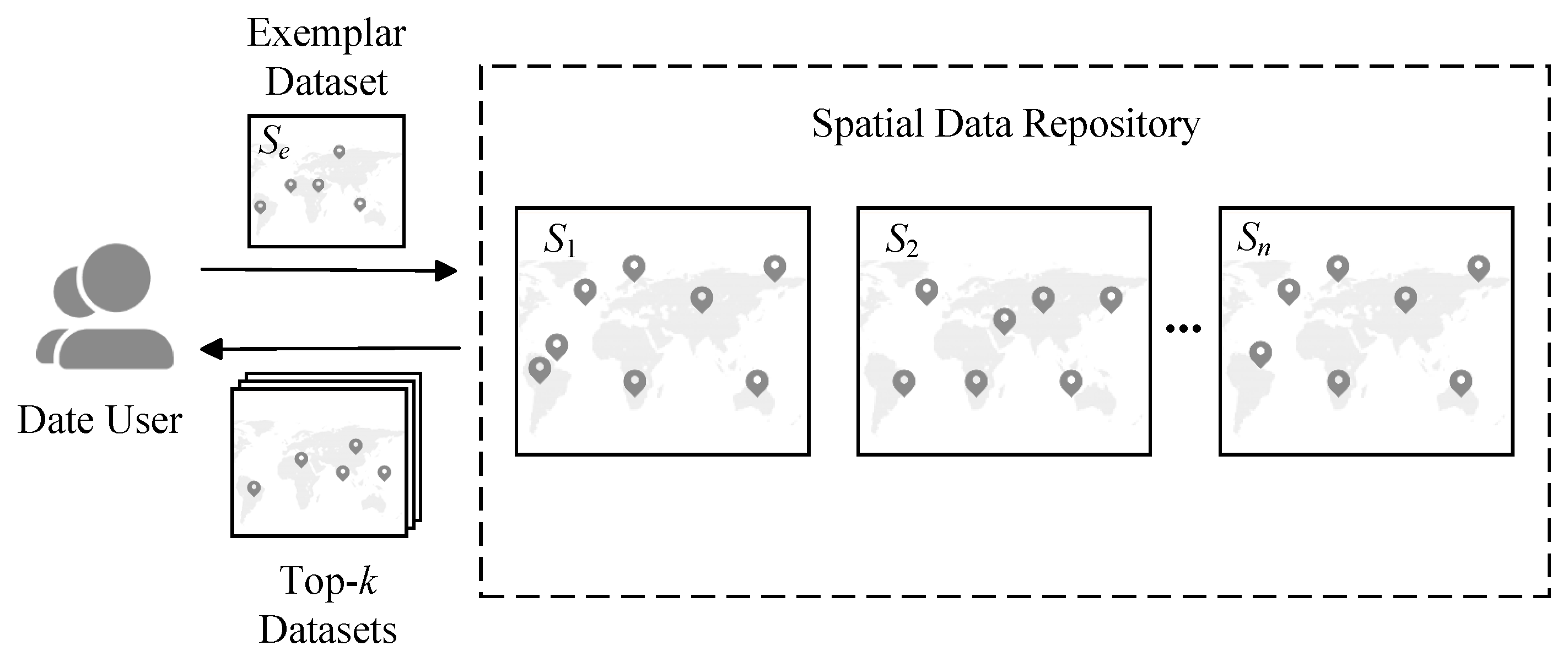
This paper focuses on the top-k spatial dataset search, which allows users to submit an exemplar dataset $S_e$ as a search query and retrieves the k spatial datasets most similar to the exemplar dataset from a spatial data repository $\mathcal{S}=\{S_1,S_2,\cdots ,S_n\}$, as illustrated in Figure 1. For example, in the Auctus search system [7], users can upload a one-month bicycle-usage dataset as an exemplar dataset to retrieve related datasets for other months, enabling the establishment of robust models for prediction tasks. In RONIN [8], users can utilize an example dataset concerning smart cities to find additional datasets that are joinable, based on the set-containment relationships between datasets. Degbelo et al. [9] introduce the Hausdorff distance into the dataset search, providing a metric to quantify the maximum deviation between two sets of location points. Yang et al. [10] employ Earth Mover’s Distance, a widely recognized metric for comparing distributions, to quantify the similarity between datasets for top-k searches. Exemplar search has emerged as a promising trend in spatial dataset search. Moreover, methods employing the Hausdorff Distance face the impact of outliers, which can affect the accuracy of the search results. On the other hand, the Earth Mover’s Distance provides more fine-grained similarity measurements, but it incurs substantial computational costs [11]. Striking a balance between the effectiveness and efficiency of similarity calculations continues to be a significant challenge.

In this paper, we propose an efficient top-k spatial dataset search processing, which can retrieve the k most similar spatial datasets to a given exemplar dataset. First, a density distribution-based similarity model (DDSM) is designed to measure the similarity between spatial datasets, which applies grid partition to compress spatial datasets into density and quantity distributions for similarity calculation. Based on the DDSM model, a baseline spatial dataset search scheme (KSDS) is proposed. It traverses each dataset in the spatial data repository and calculates its similarity to the exemplar dataset to obtain the top-k datasets with the highest similarity. To improve search efficiency, an optimized spatial dataset search scheme (KSDS+) is designed, which contains two optimization strategies to filter out datasets that are unlikely to appear in the search result. The optimized scheme also supports dynamic update operations on the spatial data repository. Experimental results on two real-world data repositories show that the proposed search-processing performs well in search effectiveness and efficiency.

The contributions of this paper are as follows.

• We propose a density distribution-based similarity model (DDSM), which uses grid partition to compress spatial datasets into density and quantity distributions to measure similarity between datasets (see Section 4).
• We propose a baseline top-k spatial dataset search scheme (KSDS) that uses DDSM for similarity calculation to obtain search results (see Section 5).
• We propose an optimized top-k spatial dataset search scheme (KSDS+), which integrates two optimization strategies to filter datasets, thereby improving search efficiency (see Section 6).
• We conduct comprehensive experiments to evaluate the proposed KSDS and KSDS+ on two real-world spatial data repositories, and the result shows the good performance of the proposed schemes (see Section 7).

This paper is organized as follows. Section 2 reviews related work and discusses existing approaches to top-k spatial dataset search. Section 3 introduces the paper’s notations, problem formulation and system model. Section 5 presents a baseline top-k spatial dataset search scheme, while Section 6 proposes an optimized search scheme to improve search performance. Section 7 presents a comprehensive evaluation of the proposed search schemes. Finally, Section 8 concludes the paper and outlines potential directions for future research.

2. Related Work

Various spatial dataset search schemes have been proposed to address different real-world business needs, such as keyword-based spatial dataset search, range search-based spatial dataset search and top-k spatial dataset search.

• Keyword-based spatial dataset search. Keyword-based dataset search is used to retrieve data points or objects associated with specific terms or keywords, much like traditional text-based search engines. A typical example would be searching a dataset with geographic information such as places, landmarks or geographic features, where users enter keywords like “park” or “restaurant” to find corresponding locations. To provide a comprehensive understanding of spatial keyword search, Chen et al. [12] conduct a comprehensive survey of existing studies on spatial keyword search. Luo et al. [13,14] propose a new query type termed instant error-tolerant spatial keyword queries on road networks and then present a real-time query system called TASKS for instant error-tolerant spatial keyword queries on road networks. Xu et al. [15] introduce a new type of query called the moving collective spatial keyword query (MCSKQ). Although keyword search is intuitive and efficient for retrieving spatial data based on textual descriptions, it lacks spatial awareness and relies heavily on exact keyword matching.
• Range-based spatial dataset search. Range-based dataset search is a type of query operation in spatial data processing that involves retrieving all data points or objects within a specified geographic range. Jin et al. [16] propose a set of five analysis methods to estimate the selectivity and the number of index nodes accessed in serving a range query. Zacharatou et al. [17] propose a novel indexing structure STITCH that efficiently executes spatial range queries on multiple datasets. Li et al. [18] propose a dictionary partition-based multi-keyword ranked search scheme that compresses vector dimensions, employs a double-tier index for efficient searches and safeguards user privacy over encrypted cloud data. Range search effectively retrieves all spatial objects within a specified geographic boundary, making it useful for location-based services.
• Top-k spatial dataset search. The top-k spatial dataset search introduces a novel query paradigm that considers a user query as an example of the data in which the user is interested [19,20,21]. Mottin et al. [22] provide an approximate solution that prunes the search space and achieves considerably better time performance with minimal or no impact on effectiveness. Yang et al. [10] tackle spatial dataset search using Earth Mover’s Distance (EMD) to measure the similarity between datasets and propose a Dual-Bound Filtering (DBF) framework to accelerate EMD-based spatial dataset search. Li et al. [23] design the order-preserving encrypted similarity to achieve secure similarity calculation and propose the baseline search scheme PriDAS and the optimized search scheme PriDAS+. Mottin et al. [24] demonstrate the functionality of a query engine XQ, which enables top-k spatial dataset search and shows its applicability in various situations. However, existing research on top-k spatial dataset search is insufficient, and it struggles to provide efficient and effective search results when dealing with large-scale spatial datasets. For example, the Hausdorff distance-based spatial dataset search is sensitive to outliers and also faces privacy restrictions in certain scenarios [25]. Additionally, the EMD-based spatial dataset search is computationally complex and incurs a significant time cost when dealing with large spatial datasets. Therefore, developing more efficient top-k spatial dataset search schemes has become crucial for improving system performance and meeting practical demands.

In this paper, we focus on top-k spatial dataset search. We integrate advanced similarity metrics with efficient indexing techniques, achieving high search effectiveness while substantially reducing computational overhead.

3. Notations, System Model and Problem Description

In this section, we begin by introducing the notations used throughout the paper to ensure consistent terminology. Then, we present the system model, which outlines the process by which the parties collaborated to complete the search for spatial datasets. Finally, we formally define the problem that we want to solve.

3.1. Notations

The notations used in this paper are listed as follows:

• G: the two-dimensional spatial space which are equally divided into $2^u\times 2^u$ grids, $G=\left\{g_{x,y}\right|x,y\in \{1,2,\cdots ,2^u\}\}$, where u is the space-dividing threshold.
• $\mathcal{S}$: the spatial data repository contains a set of spatial datasets, $\mathcal{S}=\{S_1,S_2,\cdots ,S_n\}$.
• $S_i$: the spatial dataset in $\mathcal{S}$ contains $m_i$ location points, $S_i=\{p_{i,1},p_{i,2},\cdots ,p_{i,m_i}\}$, where $p_{i,j}\in S_i$ is a location point.
• $S_e$: the exemplar spatial dataset of a top-k spatial dataset search processing.
• $D_i$: the grid distribution representation of the spatial dataset $S_i$, which consists of a set of triples.
• $E_i$: the grid-based minimum bounding rectangle (GMBR) of the spatial dataset $S_i$, which is composed of the minimum grids just covering all locations of $S_i$.
• ${\mathcal{I}}^{ϵ}$: the $ϵ$-pooling index for the spatial data repository, which consists of a two-layer indexing structure.

3.2. System Model

In this paper, we design a system model involving two parties: the data owner and the data user. They cooperate with each other to accomplish top-k spatial dataset searches.

• The data owner owns the spatial data repository and provides a search engine for the data user to discover the desired spatial datasets. First, comprehensive data preprocessing is performed, which includes cleaning the raw data and constructing indexes to enhance the organization and accessibility of the spatial information. Second, these indexes are leveraged to deliver efficient search services, ensuring rapid query responses and scalability.
• The data user submits an exemplar dataset to the data owner to initiate a top-k spatial dataset search. Then, the data owner performs search processing on the data repository using a search index. After finding the datasets, it returns these datasets as the search result to the data user.

3.3. Problem Description

Given a spatial data repository $\mathcal{S}$ and an exemplar spatial dataset, the top-k spatial dataset search is described as Definition 1.

Definition 1 

(Top-k Spatial Dataset Search). For an exemplar spatial dataset $S_e$, the top-k spatial dataset search is to search the k most similar spatial datasets in $\mathcal{S}$ to $S_e$, which is denoted as $Q=(\mathcal{S},S_e,k)$. Assuming that $R_Q$ is the search result of Q, $R_Q$ satisfies the following condition:

$$|R_Q|=k\wedge \forall S_i\in R_Q,S_j\notin R_Q\to sim(S_e,S_i)>Sim(S_e,S_j),$$

(1)

where $sim(S_e,S_i)$ is the similarity between $S_e$ and $S_i$. The similarity calculation between datasets will be introduced in Section 4, and the larger the similarity between two spatial datasets, the more similar they are.

The goal of this paper is to design an efficient top-k spatial dataset search processing that can obtain the top-k similar spatial datasets to a given exemplar dataset. We will design efficient optimization strategies to achieve this goal. The metrics for evaluating the search schemes’ performance are presented below.

• Search effectiveness evaluation. The evaluation metric for search effectiveness is the Mean Squared Error (MSE), which measures the distance between the search results and the exemplar dataset’s data location points. This metric helps assess the effectiveness of the search results.
• Search efficiency evaluation. The evaluation metric for search efficiency is time cost, which reflects the duration from the start of a search to the return of search results. This metric helps assess how quickly the system can process searches and deliver the relevant results.

4. Grid Distribution-Based Spatial Dataset Similarity Measurement

We assume that the two-dimensional spatial space is equally divided into $2^u\times 2^u$ grids and the grid set is $G=\left\{g_{x,y}\right|x,y\in \{1,2,\cdots ,2^u\}\}$, where $g_{x,y}$ is the grid at the x-th row and y-th column after space division.

Definition 2 

(Minimum Covered Grid Collection, MCG). Given a spatial dataset $S_i\in \mathcal{S}$, the minimum covered grid collection (MCG) of $S_i$, denoted as $M_i$, is the minimum set of girds that can cover all location points of $S_i$,

$$M_i=\left\{g_{x,y}\right|g_{x,y}\in G\wedge \exists p_{i,c}\in S_i\to p_{i,c}⋖g_{x,y}\},$$

(2)

where $p_{i,c}⋖g_{x,y}$ means that the location point $p_{i,c}$ is in the grid $g_{x,y}$. The MCG set corresponding to spatial data repository $\mathcal{S}$ is denoted as $\mathcal{M}$.

Definition 3 

(Grid Distribution Representation of Spatial Dataset). Given a spatial dataset $S_i\in \mathcal{S}$, the grid distribution of $S_i$ is a set of triples, denoted as

$$D_i=\{T_{i,1},T_{i,2},\cdots ,T_{i,|M_i|}\},$$

(3)

where $T_{i,j}\in D_i$ is a triple $(g,r,N)$, and $T_{i,j}.r$ and $T_{i,j}.N$ are the location density and the location quantity of the grid $T_{i,j}.g$, respectively. The calculation of $T_{i,j}.r$ is presented as follows,

$$T_{i,j}.r={\displaystyle \frac{T_{i,j}.N}{|S_i|}},$$

(4)

where $|S_i|$ is the number of location points of $S_i$. The grid distribution representation set corresponding to the spatial data repository $\mathcal{S}$ is denoted as $\mathcal{D}=\left\{D_i\right|S_i\in \mathcal{S}\}$.

According to Definitions 2 and 3, the minimum covered grid collection of a spatial dataset is the set of non-empty grids that have at least one location point of the spatial dataset, and only those non-empty grids are taken into the grid density distribution computation.

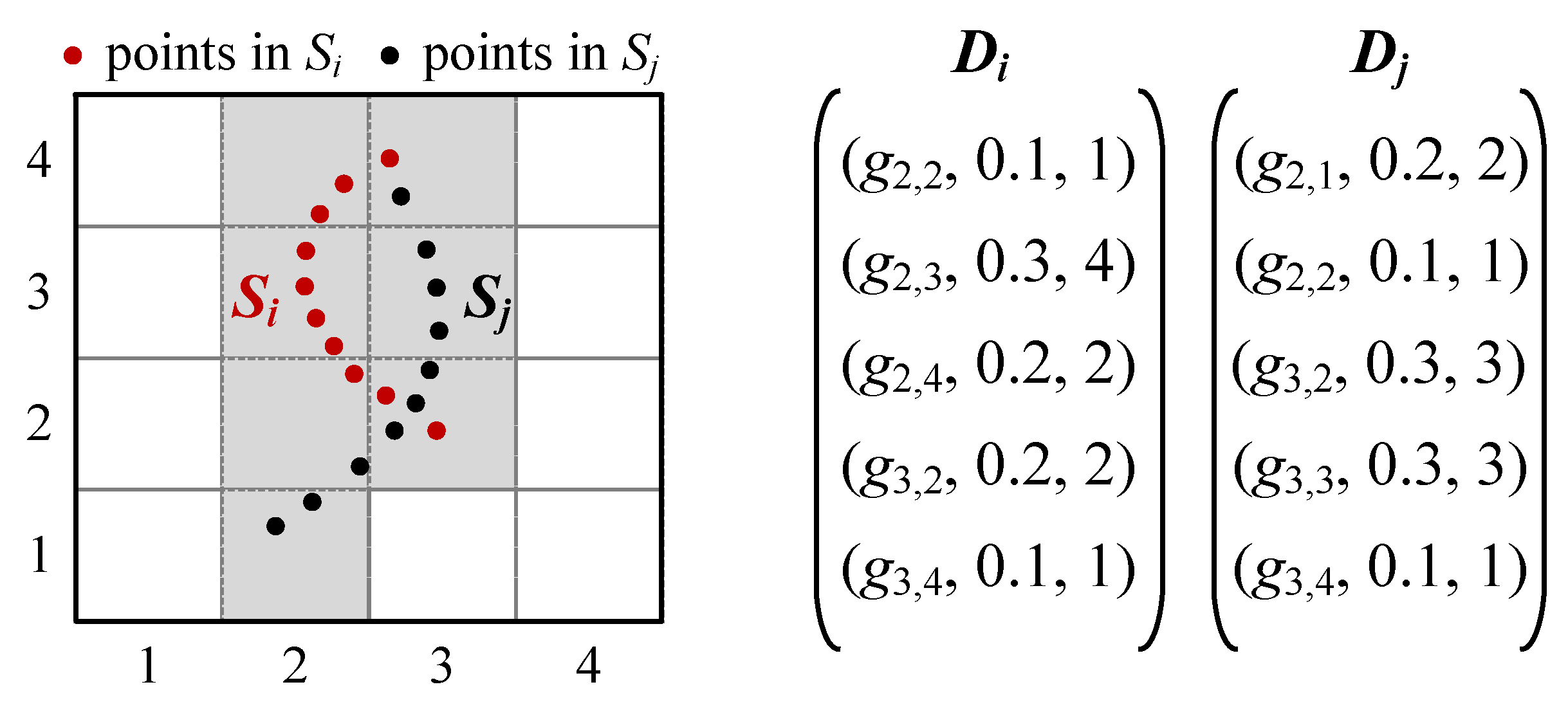
We give an example to demonstrate the above definitions shown in Figure 2. A spatial space is divided into $4\times 4$ grids, i.e., $G=\left\{g_{x,y}\right|x,y\in \{1,2,3,4\}\}$. There are two spatial datasets $S_i$ and $S_j$ distributed in G, and the corresponding grid density distributions $D_i$ and $D_j$ can be obtained by calculating the density and quantity of grids in the minimum covered grid collections $M_i$ and $M_j$, respectively.

Because the area of each grid is relatively small, points within the same grid are close to each other. For different datasets, if they have points that fall within the same grid, they have a certain degree of similarity in that grid. The similarity between two spatial datasets needs to consider both the closeness of their density distributions of spatial points and the closeness in the number of spatial points they contain. We can measure the similarity of their density distributions using the density of the overlapping grids between two datasets, and measure the similarity of the number of points using the number of overlapping grids. A similarity regulator can be introduced to regulate the weights of two types of similarity, resulting in the following definition of similarity calculation.

Definition 4 

(Grid Distribution-based Spatial Dataset Similarity, GDSS). Given two spatial datasets $S_i$ and $S_j$, and the corresponding grid distributions are $D_i$ of $D_j$, the similarity between $S_i$ and $S_j$, denoted as $sim(S_i,S_j)$, is measured as Equation (5),

$$\begin{array}{c}\hfill Sim(S_i,S_j)=\sigma DSim+(1-\sigma )QSim,\end{array}$$

(5)

where

$$DSim={\sum }_{(T_{i,x},T_{j,y})\in T}\min \{T_{i,x}.r,T_{j,y}.r\},$$

(6)

$$QSim=1-{\displaystyle \frac{|{\sum }_{(T_{i,x},T_{j,y})\in T}{T}_{i,x}.N-{\sum }_{(T_{i,x},T_{j,y})\in T}{T}_{j,x}.N|}{\max \{{\sum }_{(T_{i,x},T_{j,y})\in T}{T}_{i,x}.N,{\sum }_{(T_{i,x},T_{j,y})\in T}{T}_{j,x}.N\}}},$$

(7)

$$T=\left\{(T_{i,x},T_{j,y})\right|T_{i,x}\in D_i,T_{j,y}\in D_j\wedge T_{i,x}.g=T_{j,y}.g\},$$

(8)

σ is a similarity regulator, and $\min \{\ast \}$ and $\max \{\ast \}$ are to obtain the minimum and maximum values of a set, respectively.

Definition 4 indicates that the densities and quantities of overlapping non-empty grids are incorporated into the measurement of spatial dataset similarity. For two spatial datasets, their density distribution similarity and quantity distribution similarity in the MCG are considered. Furthermore, the similarity regulator $\sigma$ can adjust the ratio of density to quantity similarity. A higher $\sigma$ value places greater emphasis on density similarity, whereas a lower $\sigma$ emphasizes quantity similarity. The introduction of the similarity regulator enhances flexibility, allowing for adaptation to a broad spectrum of real-world requirements.

We also take the same example to illustrate Definition 4 as shown in Figure 2. For the datasets $S_i$ and $S_j$, there are three overlapping non-empty grids, $g_{2,2}$, $g_{3,2}$ and $g_{3,4}$. Different similarity regulators yield varying levels of similarity. Assuming that the similarity regulators are set at 0.5 and 0.8, the similarities between datasets $S_i$ and $S_j$ are calculated as follows: when the regulator is 0.5, the similarity $sim(S_i,S_j)=0.5\times 0.4+0.5\times 0.8=0.6$; and when the regulator is 0.8, the similarity $sim(S_i,S_j)=0.8\times 0.4+0.2\times 0.8=0.48$, according to Equation (5).

In summary, the GDSS can demonstrate the distribution feature of locations in spatial datasets by dividing the space into grids. Compared to MBR-based similarity, it provides a more detailed representation of spatial datasets, and compared to EMD-based similarity, it avoids complex similarity calculations. In practice, if smaller grids are generated by dividing the spatial space, the closer the similarity between points located in the same grid is, and the more fine-grained spatial dataset similarity measurement is achieved. However, the computational cost of the similarity calculation will be increased. We will perform experiments to evaluate the impact of space-dividing resolution in Section 7.

5. The Baseline Search Scheme

In this section, we propose a baseline top-k spatial dataset search scheme (KSDS), which utilizes the proposed similarity-calculation model GDSS to measure the similarity between spatial datasets. The baseline search scheme involves comparing an exemplar dataset with a collection of spatial datasets using the GDSS model to calculate their similarities. Consequently, a set of k ranked datasets are returned as the final search results, which are most similar to the exemplar dataset.

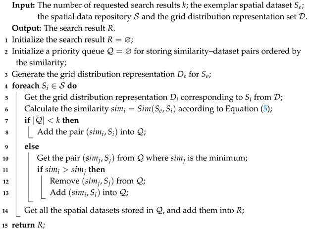
In the baseline search scheme, when a top-k spatial dataset search is initiated by the data user, the data owner performs the search processing as follows: each spatial dataset in the data repository is traversed, and the similarity between the spatial dataset and the input exemplar dataset is calculated. The k spatial datasets with the highest similarity values to the exemplar dataset are selected as the search result and returned to the data user. The details of the baseline search scheme are outlined in Algorithm 1.

In Algorithm 1, the grid distribution representation of the input exemplar spatial dataset is first generated. A priority queue is then initialized to store each spatial dataset along with its similarity to the exemplar spatial dataset. Next, for each spatial dataset in the data repository, the similarity between the spatial dataset and the exemplar spatial dataset is calculated based on Definition 4. Afterward, the spatial dataset and its similarity are considered for insertion into the priority queue. A new similarity–dataset pair is inserted, and the queue is updated only if the number of pairs in the priority queue is less than k, or if the minimum similarity in the queue is lower than the newly calculated similarity. Finally, the spatial datasets in the queue are the search results.

According to the procedures of the search processing, the time complexity of the baseline search algorithm (KSDS) is $O\left(n(\alpha \beta +\log k)\right)$, where n is the number of spatial datasets in the repository, k is the number of requested search results and $\alpha$ and $\beta$ are the average numbers of grids in MCG of the exemplar dataset and spatial datasets, respectively.

Algorithm 1: KSDS(k, $S_e$, $\mathcal{S}$, $\mathcal{D}$)

6. The Optimized Search Scheme

In this section, we propose an optimized top-k spatial dataset search processing (KSDS+), which adopts two optimization strategies to accelerate dataset filtering processing and improve search efficiency.

6.1. The Ideas of Search Optimization

The baseline search scheme involves traversing each dataset in the data repository to calculate the similarity to the exemplar dataset. However, certain datasets have distributions that are vastly different from that of the exemplar dataset (for example, the exemplar dataset is located in the Arctic, while some datasets are in the Antarctic), resulting in a similarity score of zero. Therefore, these clearly unrelated datasets can be directly filtered out without any similarity calculation. Based on this observation, we present the ideas of search optimization from two aspects:

• If we can present a more efficient filtration strategy that requires only linear time to determine whether or not a dataset should be filtered out, then we can filter out parts of the datasets efficiently to reduce the time cost.
• If we can present a more effective filtration strategy that dynamically scales the grid divisions and compares the distribution of points on the same grid for two datasets, then we can filter out parts of the dataset and thus reduce the search time overhead.

Inspired by the above ideas, we proposed two optimization strategies: GMBR-based optimization strategy and pooling-based optimization strategy, which can accelerate the top-k spatial dataset search processing.

6.2. GMBR-Based Optimization Strategy

The closer spatial datasets tend to cover more areas of rectangle overlap. For an exemplar dataset and a spatial dataset, if their minimum covering rectangles do not overlap, then the similarity between them is zero and the spatial dataset is not likely to be the final search result. We use rectangles to enclose all grids in the MCG of a spatial dataset and propose an optimization search strategy.

Definition 5 

(Grid-based Minimum Bounding Rectangle, GMBR). Given a spatial dataset $S_i\in \mathcal{S}$ and its corresponding MCG $M_i$, the GMBR of $S_i$ is a rectangle just covering all grids in $M_i$. Assuming that the bottom-left and upper-right grids in the rectangle are $g_{x,y}$ and $g_{u,v}$, respectively, the GMBR can be represented as a coordinate pair,

$$E_i=\{(x,y),(u,v)\}.$$

(9)

The GMBR set corresponding to the spatial data repository $\mathcal{S}$ is denoted as $\mathcal{E}=\left\{E_i\right|S_i\in S\}$.

Lemma 1. 

Assuming that $S_i$ and $S_j$ are two spatial datasets, and $E_i$ and $E_j$ are the corresponding GMBRs, respectively, when $E_i$ and $E_j$ have no overlap GMBR area, the similarity between $S_i$ and $S_j$ is 0, i.e.,

$$Sim(S_i,S_j)=0.$$

(10)

Proof. 

According to Definition 5, if $E_i$ has no overlap GMBR area with $E_j$, then for any grids $g_{x,y}\in E_i$, we have $g_{x,y}\notin E_j$. Thus, according to the similarity calculation in Definition 4, T is an empty set and thus $DSim$ and $QSim$ are both 0, leading to $Sim(S_i,S_j)=0$. Thus, Lemma 1 is proved.    □

According to Lemma 1, for any spatial dataset $S_i$, if it has no overlapping area with the GMBR of the exemplar dataset $S_e$, the similarity between them is zero. During the dataset search processing, such datasets contribute nothing to the search result and can be filtered out directly without any similarity calculation. Thus, the GMBR-based optimization strategy can be used to filter out spatial datasets with zero similarity to the exemplar dataset. The details of the overlap check processing are outlined in Algorithm 2.

Algorithm 2: CheckGMBR($E_i$, $E_e$)

In Algorithm 2, the GMBRs of the spatial dataset in the data repository and the exemplar dataset are inputted and their bottom-left and upper-right coordinates are used to check if there is overlapping GMBR area. If there is, the output is $true$, otherwise $false$, thereby reducing the number of similarity calculations and improving search efficiency. By checking whether the GMBRs overlap, we can quickly filter out datasets that are unlikely to be search results, thereby reducing the number of similarity calculations and improving search efficiency.

6.3. Grid Pooling-Based Optimization Strategy

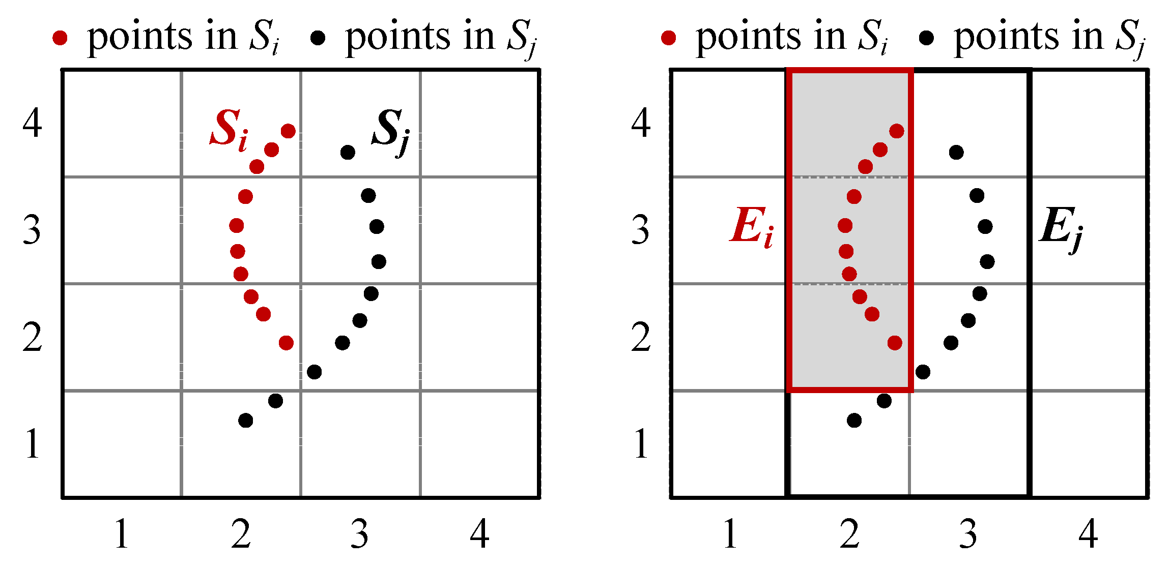
The GMBR-based optimization strategy can quickly filter out far-apart datasets that do not overlap with the exemplar dataset. However, there are still datasets that, despite having an overlap area with the exemplar dataset, yield a similarity score of 0. This occurs because GMBR only takes into account the proximity of the dataset as a whole, and does not take into account the proximity of the dataset in a finer-grained grid. For example, as shown in Figure 3, In cases where the similarity between two datasets is zero, which is unlikely to represent a final search result, the GMBR strategy alone proves inadequate for efficient filtering. This stems from GMBR’s aggregate-based perspective, which hinders swift exclusion of such datasets.

To achieve finer-grained filtering, we propose a pooling-based optimization strategy as follows.

Definition 6 

($ϵ$-Grid Pooling). Given a two-dimensional spatial space G which is equally divided into $2^u\times 2^u$ grids, and a grid pooling threshold ϵ$(1\le ϵ\le u-1)$, the ϵ-grid pooling performs grid pooling on G to equally generate $2^{u-ϵ}\times 2^{u-ϵ}$ grid pools, i.e.,

$$G=\left\{g_{x,y}^{ϵ}|x,y\in \{1,2,\cdots ,2^{u-ϵ}\}\right\}.$$

(11)

According to Definition 6, we have the following observations:

• Each grid pool $g_{x,y}^{ϵ}\in G$ contains $2^{ϵ}\times 2^{ϵ}$ grids.
• The grid pool $g_{x,y}^{ϵ}$ that contains grid $g_{c,j}$ can be quickly located using the equation: $(x,y)=(\lfloor {\displaystyle \frac{c}{2^{ϵ}}}\rfloor ,\lfloor {\displaystyle \frac{j}{2^{ϵ}}}\rfloor ).$

Definition 7 

($ϵ$-minimum Covered Grid Pool Collection). Given a spatial dataset $S_i\in \mathcal{S}$ and corresponding MCG $M_i$, the minimum covered grid pool collection (MCG^ϵ) of $S_i$ after ϵ-grid pooling, denoted as $M_i^{ϵ}$, is the minimum set of gird pools that can cover all grids in $MC{G}_i$ $M_i$,

$$M_i^{ϵ}=\left\{g_{x,y}^{ϵ}\right|g_{x,y}^{ϵ}\in G\wedge \exists g_{c,j}\in M_i\to g_{c,j}⋖g_{x,y}^{ϵ}\},$$

(12)

where $g_{c,j}⋖g_{x,y}^{ϵ}$ means that grid $g_{c,j}$ is in the grid pool $g_{x,y}^{ϵ}$. The MCG^ϵ set corresponding to spatial data repository $\mathcal{S}$ is denoted as ${\mathcal{M}}^{ϵ}$.

Definition 8 

($ϵ$-pooling Index). Given a spatial data repository $\mathcal{S}$ and the corresponding grid distribution representation set $\mathcal{D}$, the ϵ-pooling index ${\mathcal{I}}^{ϵ}=(I_u^{ϵ},I_l^{ϵ})$ is a two-layer index.

• The upper layer $I_u^{ϵ}$ is a set of pair $(i,P_i)$, where i is the identifier of dataset $S_i\in \mathcal{S}$ and $P_i$ is the set of grid pools in $MC{G}^{ϵ}$ $M_i^{ϵ}$ of $S_i$.
• The lower layer $I_l^{ϵ}$ is a set of pairs $(i,D_i)$, where i is the identifier of dataset $S_i\in \mathcal{S}$ and $D_i$ is the set of triples in the grid distribution representation of $S_i$ defined in Definition 3.

We give an example of the $ϵ$-pooling index, as shown in Figure 4. Figure 4a shows two spatial datasets under the $4\times 4$ space grid partitioning, Figure 4b shows the pooling results for the $ϵ=2$ case and Figure 4 shows the generated two-layer pooling index.

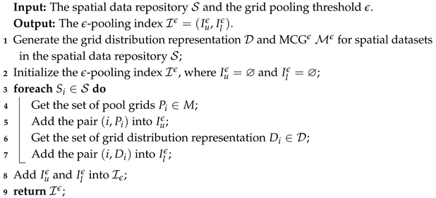
The details of building the $ϵ$-pooling index are outlined in Algorithm 3. The spatial data repository and the grid pooling threshold are taken as input, and the corresponding grid distribution representation and MCG^ϵ are generated. Then, the pairs in both the upper layer and lower layer in the index are acquired, and finally, the $ϵ$-pooling index is generated. The selection of the pooling threshold $ϵ$ affects the size of the grid pool, which in turn affects the filtering efficiency and the space cost of the pooling index. The larger the $ϵ$, the more grids each grid pool contains, resulting in lower filtering efficiency and smaller storage overhead. In practical applications, we recommend weighing the time and space overhead and setting the parameter value reasonably.

Algorithm 3: BuildIndex($\mathcal{S},ϵ$)

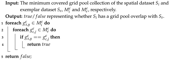
We propose a pooling-based optimization strategy based on the pooling index. The upper layer of the index can quickly determine whether a dataset overlaps with the exemplar dataset in terms of MCG^ϵ (as shown in Algorithm 4), which helps to assess whether the dataset could be part of the final search results. If the dataset does not share an overlapping MCG^ϵ with the exemplar dataset, it can be filtered out directly without the need for further similarity calculations, thereby improving search efficiency.   

Algorithm 4: CheckPool($M_i^{ϵ}$, $M_e^{ϵ}$)

6.4. The Optimized Search Algorithm

During the above optimization strategies for the baseline search scheme, the GMBR and the pooling index are used to accelerate dataset filtering, thus speeding up the search process. Adopting the above optimization strategies, we present an optimized spatial dataset search process (KSDS+). The GMBR-based optimization strategy has a lower time overhead, but cannot fine-grained filter out spatial datasets with zero similarity to the exemplar dataset, while the pooling-based optimization strategy achieves the opposite. Thus, the steps of the KSDS+ search processing we designed are as follows:

• $CheckGMBR$. Determine whether each dataset has GMBR overlap with the exemplar dataset according to GMBR-based optimization strategy.
• $CheckPool$. Assess whether each dataset has a grid pool that overlaps with the exemplar dataset according to the pooling-based optimization strategy.
• $Search$. Calculate the similarity between each dataset that satisfies the $CheckPool$ and the exemplar dataset according to GDSS, and select the top-k datasets with the highest similarity to the exemplar dataset.

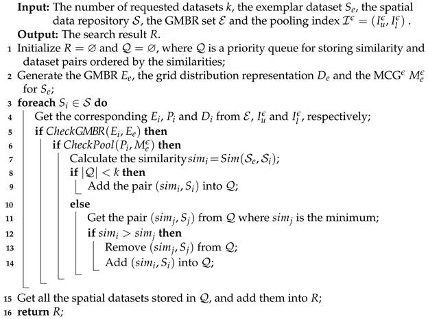
Since both of our proposed optimization strategies specifically filter out datasets with a similarity score of zero, our two optimization strategies effectively improve the efficiency of spatial dataset search while ensuring accurate search. Additionally, the GMBR-based optimization strategy has better adaptability to situations where the data repository covers a large area and the datasets are relatively scattered, while the grid pooling-based optimization strategy can make up for the shortcomings of the GMBR-based optimization strategy when the datasets are relatively concentrated. Therefore, we recommend combining these two optimization schemes in practical applications to achieve better optimization results.Based on the above analysis, we can first use the GMBR-based optimization strategy to quickly filter out datasets with zero similarity, then use the pooling-based optimization strategy to filter out the remaining datasets with zero similarity and finally perform similarity calculations to complete the search. Details of the optimized spatial dataset search processing are presented in Algorithm 5.

In Algorithm 5, the GMBR, the grid distribution representation and the MCG are first generated for the exemplar dataset. Then, for each dataset in the data repository, it is checked whether there is an overlap between its GMBR and the exemplar dataset. If an overlap exists, the dataset is further checked for overlap between its grid pool and the exemplar dataset. For each dataset that satisfies these conditions, a priority queue is then initialized to store the dataset along with its similarity to the exemplar spatial dataset. A new similarity–dataset pair is inserted, and the queue is updated only if the number of pairs in the priority queue is less than k, or if the minimum similarity in the queue is lower than the newly calculated similarity. Finally, the spatial datasets in the queue are the requested spatial datasets.

According to the search-processing procedures, the time complexity of the optimized search algorithm (KSDS+) is $O\left(n+\eta ({\alpha }^{\prime }+{\beta }^{\prime })+{\eta }^{\prime }(\alpha +\beta +\log k)\right)$. Here, ${\eta }^{\prime }$ is the number of datasets that satisfy step $CheckPool$, ${\alpha }^{\prime }$ and ${\beta }^{\prime }$ are the average numbers of grid pools in $MC{G}^{ϵ}$ of exemplar datasets and spatial datasets, respectively. The meanings of $\alpha$, $\beta$, n, k, $\eta$ are the same as in Section 5.

Algorithm 5: KSDS+(k, $S_e$, $\mathcal{S}$, $\mathcal{E}$, ${\mathcal{I}}^{ϵ}$)

6.5. Dynamic Update Operation Support

The proposed scheme KSDS+ also supports dynamic update of datasets. We introduce countermeasures for update operations, including dataset insertion and deletion. It is noticeable that a spatial dataset-modification operation can be achieved by performing a dataset deletion first and then a dataset insertion.

• Insertion. Assuming that the set of spatial datasets to be inserted is $S^{\prime }$, the specific steps of insertion are as follows.

  (1)

  A set of GMBRs are generated corresponding to $S^{\prime }$. Then, the generated GMBR set is inserted into the data repository’s existing GMBR set while maintaining the mapping between each dataset and its corresponding GMBR.

  (2)

  The grid distribution representation and MCG^ϵ are generated for each dataset in $S^{\prime }$. These are then inserted into the lower and upper layers of the pooling index.

• Deletion. Assuming that the set of spatial datasets to be deleted is $S^{\prime }$, the specific steps of the deletion are as follows.

  (1)

  The GMBR corresponding to $S^{\prime }$ is associated and removed from the set of GMBRs corresponding to the data repository.

  (2)

  The upper and lower tuples corresponding to $S^{\prime }$ in the pooling index are identified, and they are removed from the pooling index in the data repository, respectively.

In summary, KSDS+ maintains an efficient adaptive index. By supporting incremental updates, the updatability of the index ensures that this approach can be effectively applied in scenarios where data sets are constantly evolving.

7. Performance Evaluation

In this section, we first introduce the experimental settings. Then, we perform a comprehensive evaluation of the proposed search schemes KSDS and KSDS+, comparing them with the EMD-based search scheme [10]. The evaluation contains search effectiveness evaluation, search efficiency evaluation and space cost evaluation.

7.1. Settings

Datasets. The proposed schemes are evaluated on two real-world spatial data repositories, Public and Identifiable, which are collected from OpenStreetMap [10]. The details of the spatial data repositories are introduced in

Table 1. Details of spatial data repositories.

Data Repository	Storage (GB)	Number of Datasets	Number of Points
Public	29.43	546,193	13,747,735
Identifiable	19.64	235,483	13,043,935

.

• Implementation. The tested search schemes are implemented in the hardware environment with an Intel i7-8550U CPU, 128 GB memory and 1 TB hard disk and in the software environment with a 64-bit Windows 10 operating system and the Python 3.1 development kit.
• Exemplar Datasets. For each search processing, we randomly select a dataset from a spatial data repository as the exemplar dataset and take the average result of 100 searches as the final search result.
• Data preprocessing. As the data owner, we generate GMBR and MCG$ϵ$ for each spatial dataset in the repository to construct GMBRs and grid pooling indexes. These indexes efficiently organize and manage the datasets, enhancing search and retrieval processes within the spatial data repository.
• Parameter settings. The parameters include $\sigma$, k, n, u and $ϵ$, of which $ϵ$ is assigned 14 parameter values and the remaining parameters are assigned 5 experimental values. The parameter settings of our evaluations are presented in

  Table 2. Parameter settings.

  Notations	Meanings	Parameter Values
  $\sigma$	The similarity regulator	(0, 0.2, 0.5, 0.8, 1)
  k	The number of requested spatial datasets	(5, 10, 15, 20, 25)
  n	The number of spatial datasets	(2, 4, 6, 8, 10) $\times {10}^4$
  u	The space-dividing threshold	(11, 12, 13, 14, 15)
  $ϵ$	The pooling threshold	(0, 1, 2, 3, 4, …, 12, 13)

  and the underlined parameter values are the default parameter values.

7.2. Search Effectiveness Evaluation

This subsection evaluates the effectiveness of algorithms KSDS, KSDS+ and EMD for performing spatial dataset searches, with MSE as a metric to evaluate the effectiveness of search results.

To calculate the MSE, we first perform k-means clustering on the points in the exemplar dataset to determine the cluster centers. Subsequently, we compute the average distance from each point in the search results to its nearest cluster center. The MSE quantifies the average distance between the location points of the search results and those of the exemplar dataset, with a smaller MSE indicating closer proximity between the two sets of points. Since $ϵ$ is solely used to accelerate the search and does not affect the search results, experiments evaluating search effectiveness do not include the parameter a. 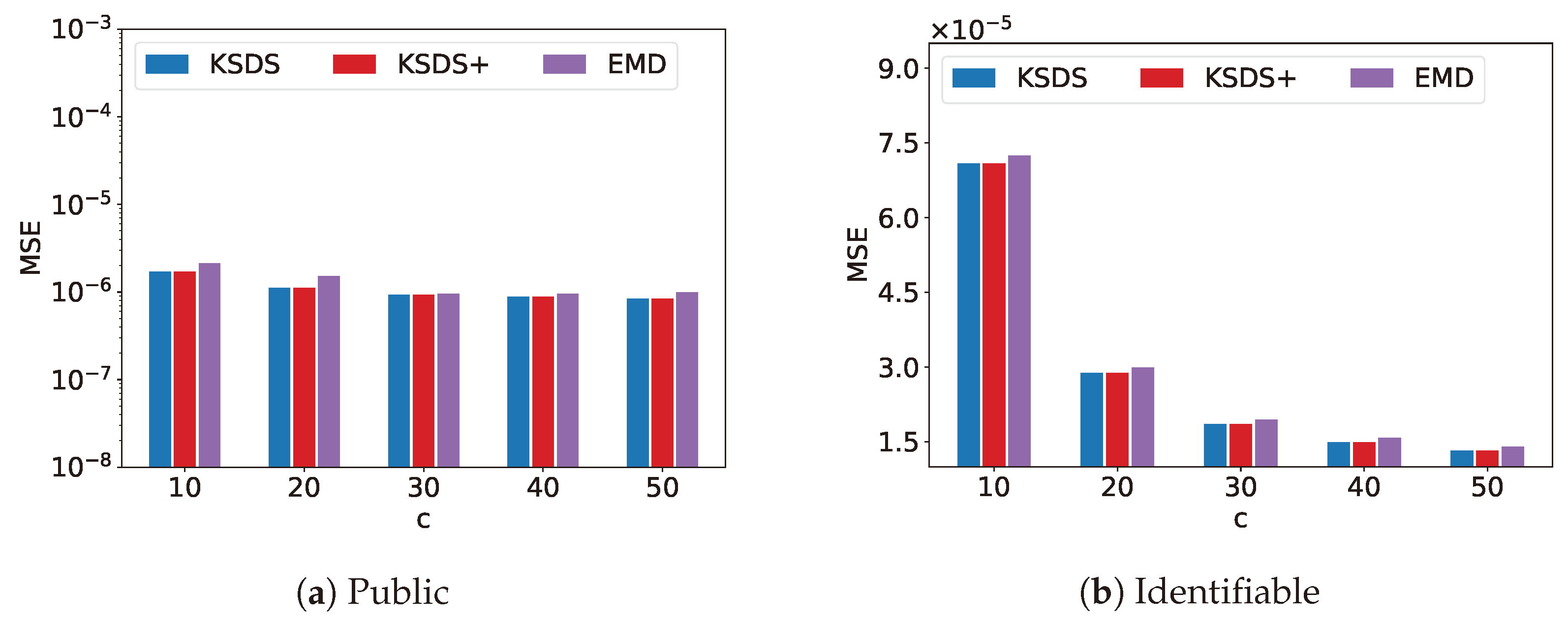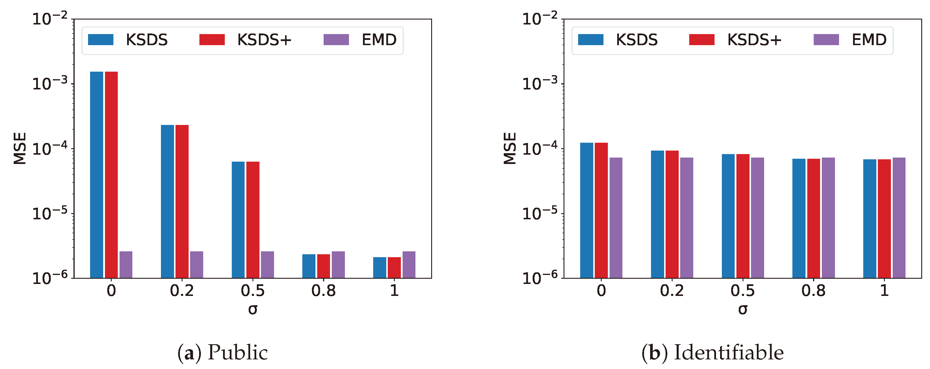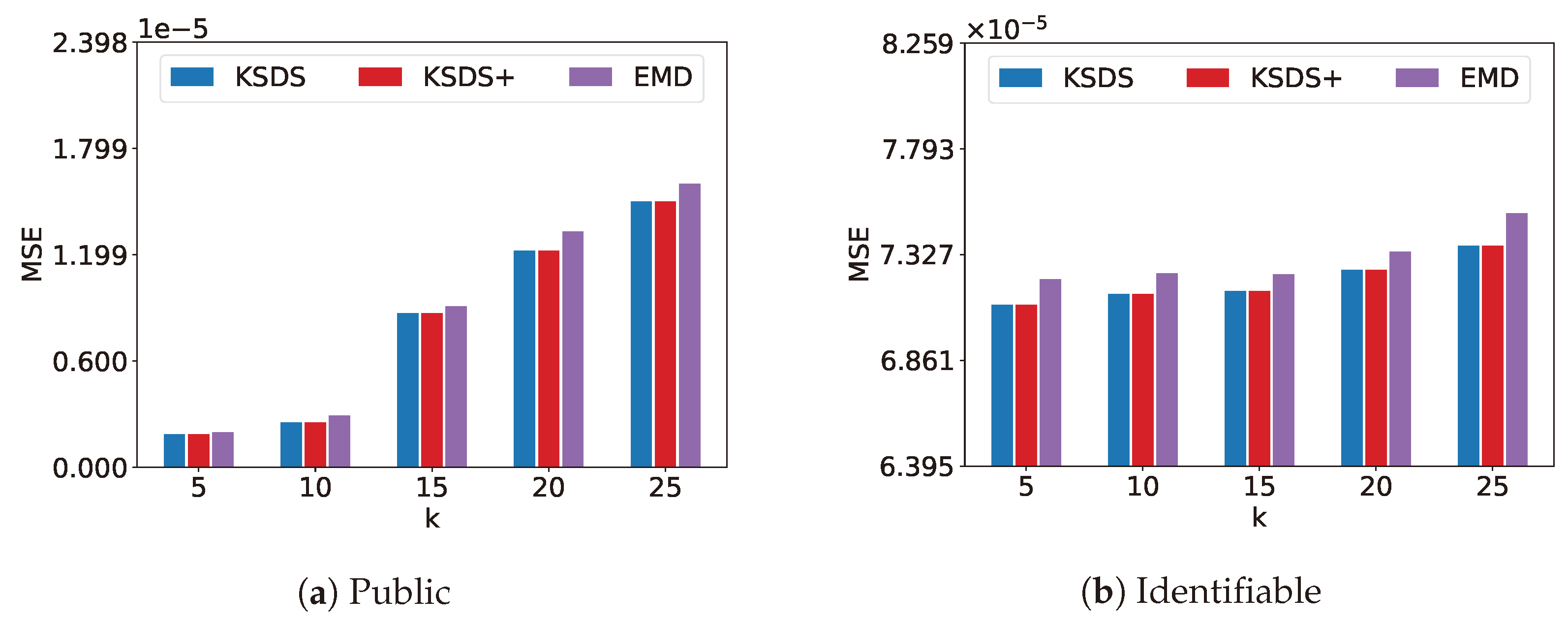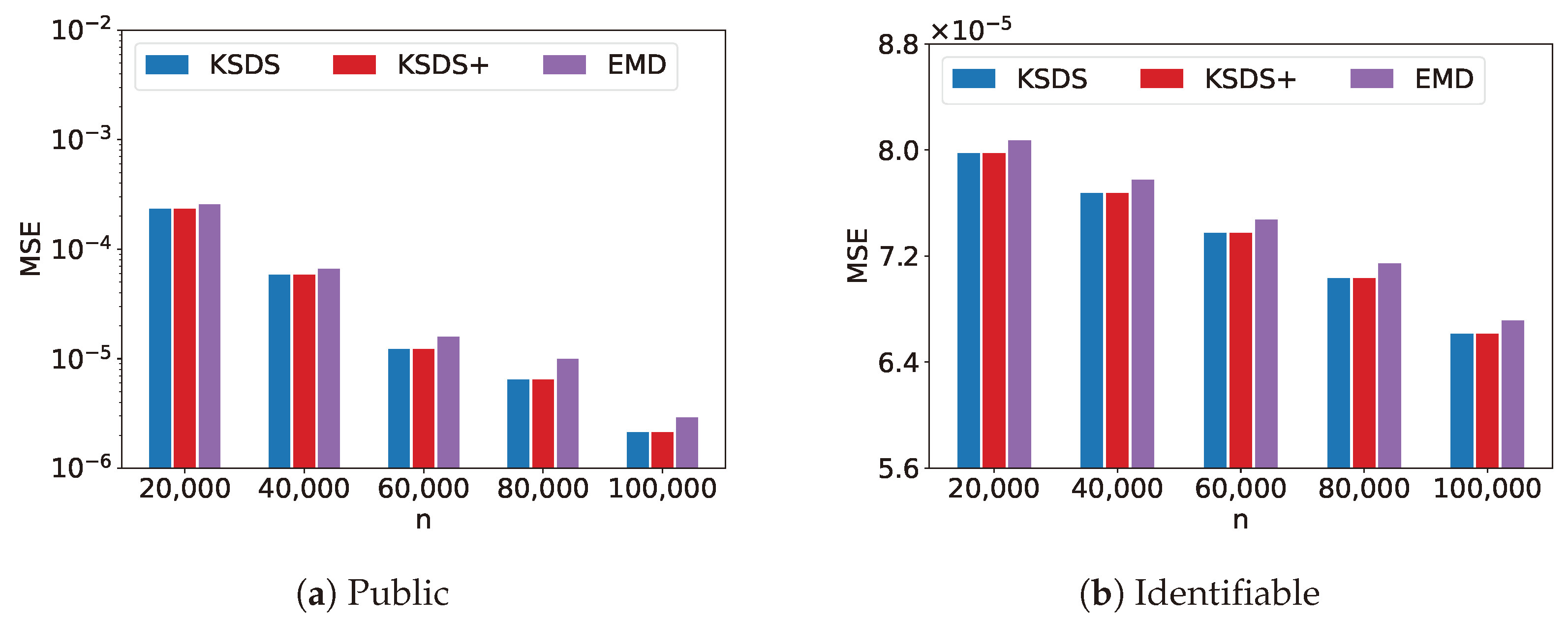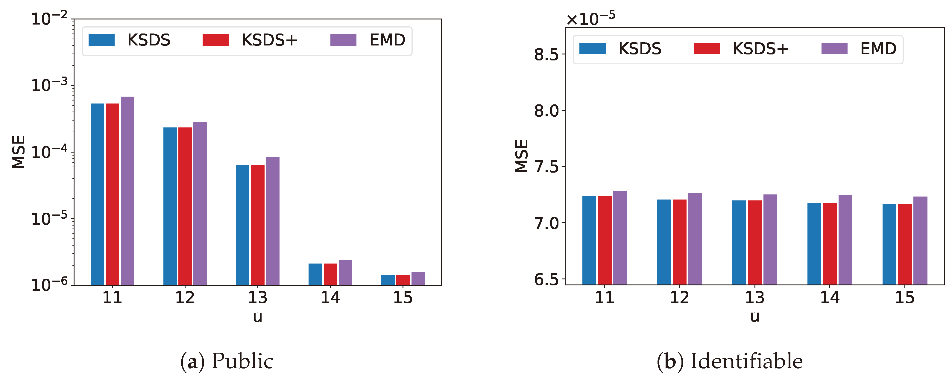Figure 5, Figure 6, Figure 7, Figure 8 and Figure 9 illustrate the MSE of KSDS, KSDS+ and EMD as the parameters c, $\sigma$, k, n and u vary.

Figure 5 compares MSE versus c for the KSDS, KSDS+ and EMD algorithms. The parameter c denotes the number of cluster centers used in clustering the search results. An increase in c implies a larger number of cluster centers, resulting in the dataset being partitioned into more categories. As c increases, the MSE values for KSDS, KSDS+ and EMD all decrease. This decrease occurs because a higher number of cluster centers reduces the average distance between the search result points and their nearest cluster center.

Figure 6 compares MSE versus $\sigma$ for the KSDS, KSDS+ and EMD algorithms. The parameter $\sigma$ serves as the similarity regulator in the similarity-calculation process. As the parameter $\sigma$ decreases, the similarity calculation increasingly emphasizes quantitative similarity. Consequently, certain points outside the intersection of MCGs may contribute to a reduction in the average distance between location points within the datasets, thereby decreasing the overall MSE.

Figure 7 compares MSE versus k for the KSDS, KSDS+ and EMD algorithms. The parameter k denotes the number of requested spatial datasets. As k increases, the MSE of KSDS, KSDS+ and EMD algorithms also increase. This is because a larger k results in the inclusion of more datasets with lower similarity in the search results, thereby leading to higher MSE values.

Figure 8 compares MSE versus n for the KSDS, KSDS+ and EMD algorithms. The parameter n denotes the number of spatial datasets. As n increases, the MSE values of algorithm KSDS, KSDS+ and EMD all decrease. This occurs because a larger number of datasets in the data repository enhances the likelihood of finding more similar results, thereby decreasing the MSE.

Figure 9 compares MSE versus u for the KSDS, KSDS+ and EMD algorithms. The parameter u denotes the space-dividing threshold used in the grid partitioning process. The parameter u directly determines the number of grids within each dataset’s MCG, thereby affecting the computational time overhead for each similarity calculation. As illustrated in the figure, a larger u results in increased search time cost.

From Figure 5, Figure 6, Figure 7, Figure 8 and Figure 9, it can be observed that KSDS and KSDS+ exhibit the same MSE. This is because KSDS+ primarily functions as a filtering mechanism, eliminating datasets that are unlikely to be part of the final search result, without affecting the accuracy compared to KSDS. Additionally, the results demonstrate that both KSDS and KSDS+ achieve consistently lower MSE values compared to EMD. This indicates that our proposed methods are more effective in maintaining accuracy while optimizing the top-k search process, further validating their advantages.

7.3. Search Efficiency Evaluation

This subsection evaluates the effectiveness of KSDS, KSDS-GMBR, KSDS-Pooling, KSDS+ and EMD for performing spatial dataset searches. The search efficiency of five schemes is evaluated, where KSDS is the baseline search scheme, KSDS+ is the optimized search scheme and KSDS-GMBR and KSDS-Pooling are the addition of GMBR-based and Pooling-based optimization strategies to the baseline scheme, respectively. 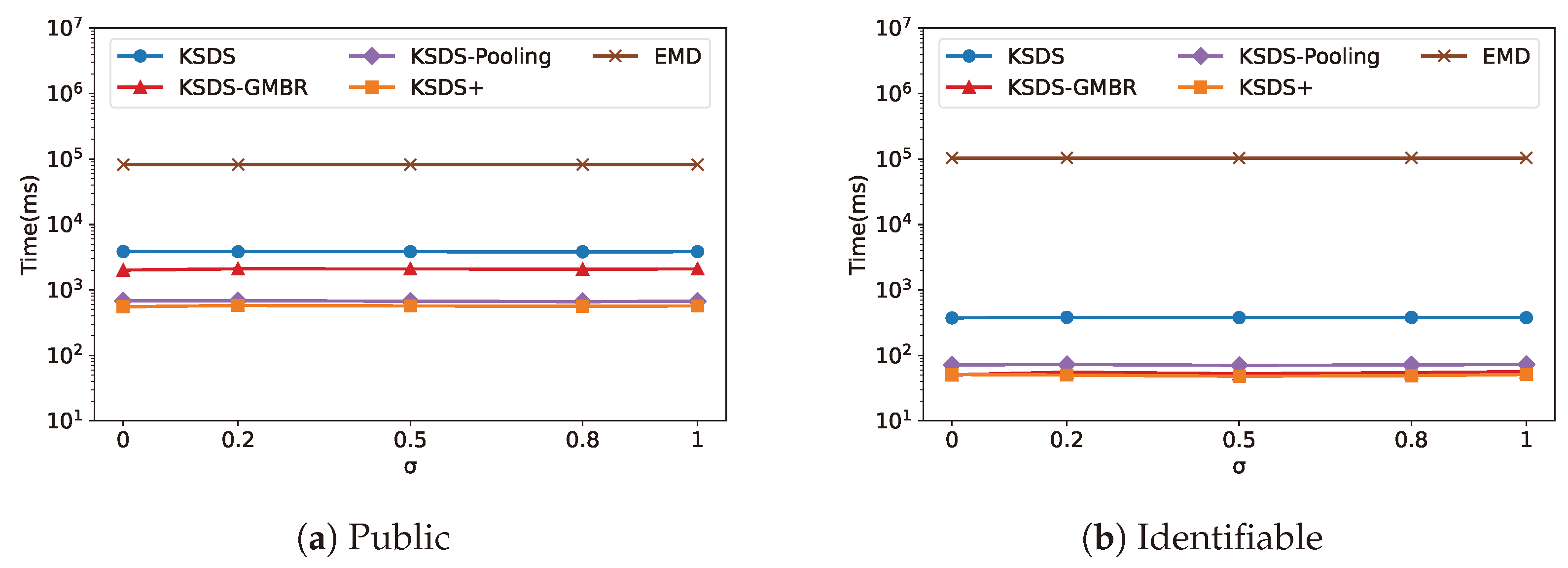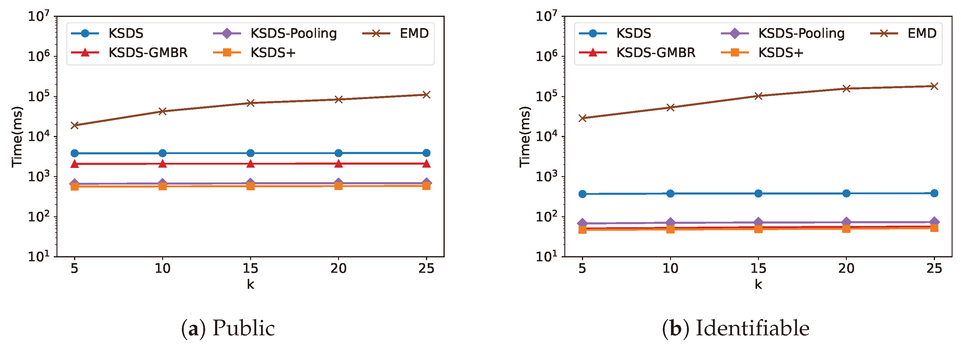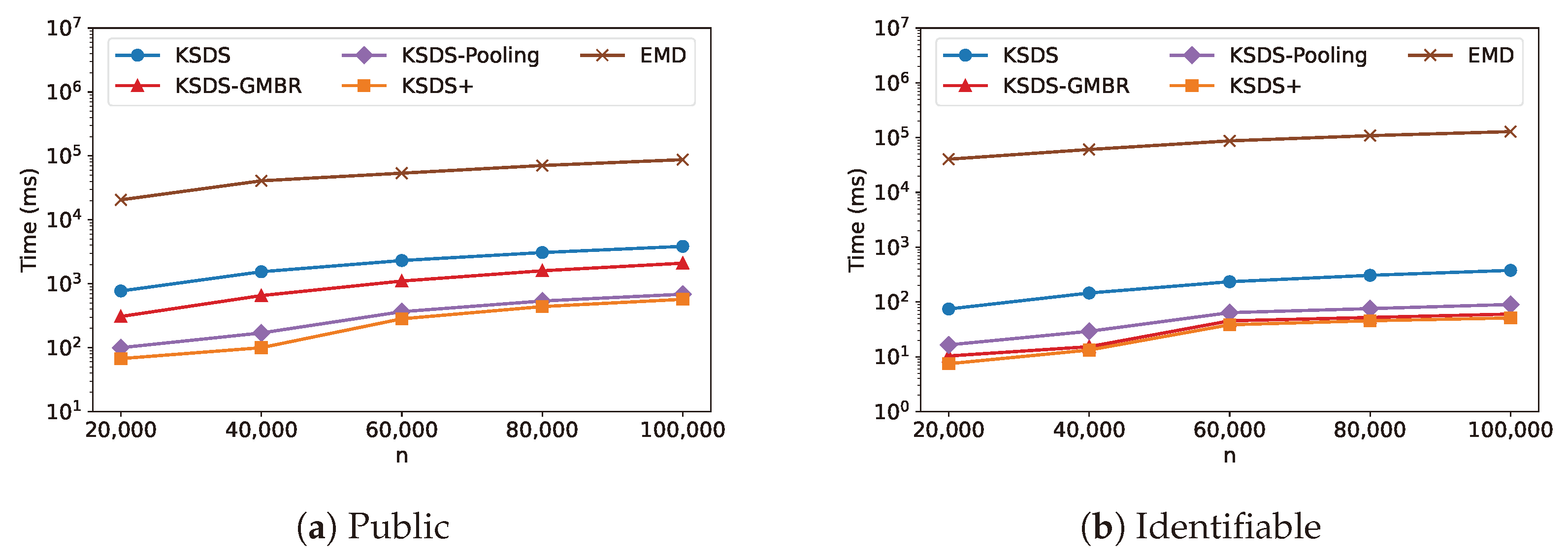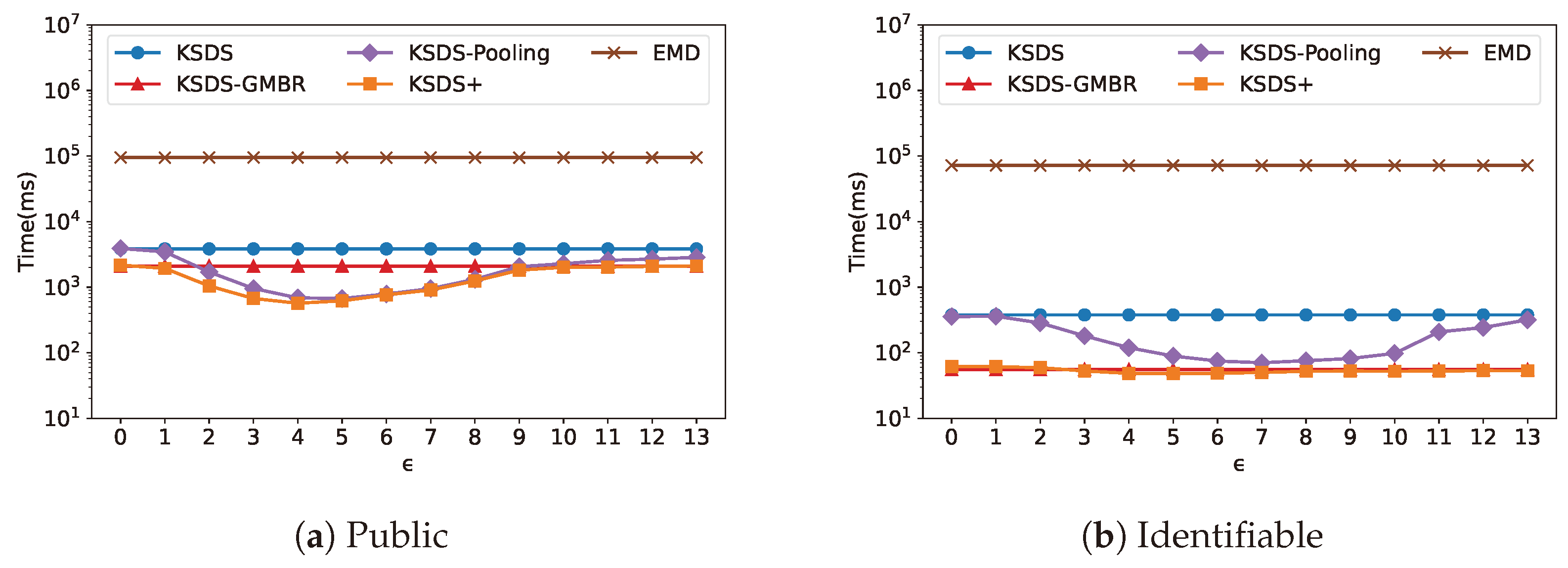Figure 10, Figure 11, Figure 12, Figure 13 and Figure 14 illustrate the search time cost of KSDS, KSDS+ and EMD as the parameters $\sigma$, k, n, u vary.

The variation in the search time cost with $\sigma$ is shown in Figure 10, from which it can be concluded that the difference $\sigma$ has almost no effect on search efficiency. This is because $\sigma$ only affects the result of similarity calculation between datasets, but not the efficiency of similarity calculation, and thus does not affect the spatial dataset search efficiency.

The variation in the search time cost with k is shown in Figure 11, from which it can be concluded that the search time cost is almost the same at different k. This is because k is only used in the sorting phase to select the top-k similarity datasets. However, the time overhead of the sorting phase is only a very small fraction of the time overhead of the total search. Therefore, the different k has little effect on the spatial dataset search efficiency.

The variation in the search time cost with n is shown in Figure 12, from which it can be concluded that as the number of datasets n increases, the search time cost increases. This is because increasing n incurs more similarity calculations, which reduces the search time cost.

The variation in the search time cost with u is shown in Figure 13, from which it can be concluded that as the grid threshold u increases, the search time overhead increases. This is because an increase in u divides the spatial space into more grids, requiring more grids to be involved in similarity calculation. This increases the time cost of similarity calculation and, therefore, decreases the search efficiency.

The relationship between search time cost and $ϵ$ is illustrated in Figure 14. It can be observed that the search efficiency of KSDS and KSDS-GMBR remains unchanged as $ϵ$ varies. This is because $ϵ$ only influences KSDS-Pooling and KSDS+, thereby affecting their search efficiency. As $ϵ$ changes, the search efficiency of KSDS-Pooling and KSDS+ exhibits a decreasing trend followed by an increase. From the results, we identify the optimal values of $ϵ$ that minimize the search time overhead for the two data repositories, Public and Identifiable, which are $ϵ=4$ and $ϵ=7$, respectively.

From Figure 10, Figure 11, Figure 12, Figure 13 and Figure 14, it can be observed that under the default parameters, KSDS+ consistently achieves the highest search efficiency. KSDS-GMBR and KSDS-Pooling exhibit different optimization capabilities, with their effectiveness varying across different datasets. Specifically, KSDS-GMBR demonstrates superior optimization performance when datasets in the data warehouse are spatially distant from each other. Meanwhile, KSDS-Pooling enhances search efficiency when datasets are spatially close to each other and contain sparse internal data points. Therefore, the combined use of these two approaches is a good choice to enhance search performance.

7.4. Space Cost Evaluation

This subsection evaluates the pooling index space cost for performing spatial dataset searches. We mainly consider the space cost changes induced by the pooling index when the pooling threshold changes and select the appropriate pooling threshold in conjunction with the evaluation of the search efficiency in Figure 14.

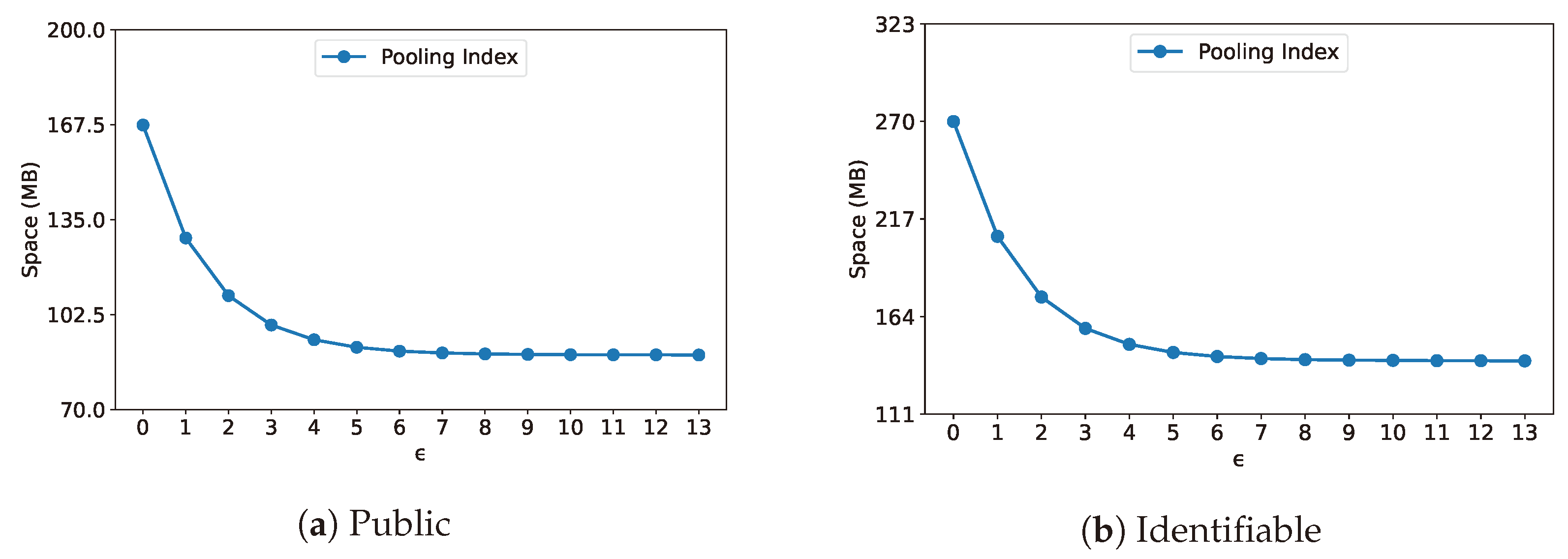
The relationship between the space cost of the index is depicted in Figure 15. As $ϵ$ increases, the index space cost also increases because a finer grid partition creates more index entries, consuming more storage. This means that choosing $ϵ$ is not just about improving search speed, it also impacts memory usage. If $ϵ$ is too small, the search efficiency may decrease, while a larger $ϵ$ can lead to unnecessary storage overhead. In real-world applications, it is important to find a good balance based on the dataset and performance needs. In this experiment, Figure 14 and Figure 15 are combined to evaluate the parameter settings and the default parameter value is set to 4 as it strikes a good balance between search performance and memory overhead. This choice ensures efficient query processing while keeping storage consumption reasonable.

8. Conclusions

In this paper, we propose two spatial dataset search schemes, KSDS and KSDS+, for the problem of top-k spatial dataset search. The primary innovation of our scheme is to divide the spatial dataset into grids and measure the similarity between spatial datasets using the distribution of points in the dataset on the grids. Then, we introduced a GMBR-based optimization strategy and a pooling-based optimization strategy to accelerate spatial dataset filtering efficiency. The experimental results demonstrated that our schemes can efficiently perform top-k spatial dataset search, outperforming existing approaches in search efficiency. In the future, we plan to explore other faster similarity-calculation models, the application of our proposed schemes on various datasets and experiment with privacy-preserving techniques to ensure the security of dataset searches. These advances aim to improve the applicability and efficiency of spatial dataset search in real-world scenarios.