An Inference Framework of Markov Logic Network for Link Prediction in Heterogeneous Networks

Abstract

The presence of multiplex edges and sparse links often hampers the efficacy of link prediction (LP) tasks. By harnessing the expressive power of Markov logic network (MLN) formulations, multiplex edges can be unified to enhance LP effectiveness. However, scaling up inferences for effective LP remains challenging due to the inefficiency of traditional MLN inference methods. To tackle this issue, we redefine LP tasks within heterogeneous networks using MLN inferences and introduce a tailored inference framework to handle unobserved nodes and complex MLN structures. We propose a method to partition the MLN structure into discrete substructures and compute node label distributions using the variational expectation maximization (VEM) algorithm. Additionally, we establish a termination condition to streamline inference search space and present the MLN-based LP algorithm. Experimental findings demonstrate the efficacy of our VEM-driven MLN inference framework for LP tasks in heterogeneous networks, showcasing superior accuracy compared to existing approaches.

1. Introduction

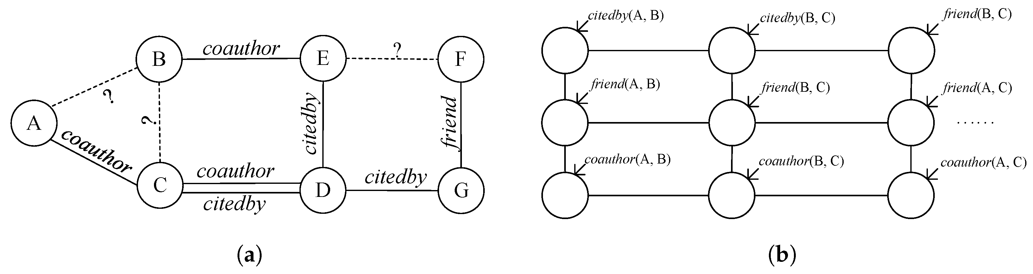
Link prediction (LP) in heterogeneous networks (also known as multi-relational LP) [1] aims to forecast multi-type connections between objects in networks. This field has recently garnered significant interest due to its diverse applications in social networks [2], knowledge graph completion [3], community discovery [4], item recommendation [5], etc. For instance, in a heterogeneous academic social network with entities like authors A, B, and C and link types such as coauthor and citedby, as illustrated in Figure 1a, the LP task involves determining the validity of links like coauthor (A, B), citedby (A, B), and citedby (B, C). Notably, these diverse link types mutually influence each other’s existence, such as citedby (C, D) impacting coauthor (C, D). Moreover, the scarcity of observed links compared to potential links results in the link sparsity challenge.

LP in heterogeneous networks faces two primary challenges. Firstly, nodes in such networks often exhibit multiple relationship types, necessitating the creation of a unified metric space that captures the inter-dependencies among these diverse links [6]. Current approaches [7,8] typically extract and merge type-specific features into distinct metric spaces, aiming to enhance prediction performance through transfer learning or algebraic space integration. However, these methods often neglect dependencies across various link types, leading to decreased accuracy. For instance, the presence of a coauthor link between C and D might influence citedby. Secondly, real-world networks exhibit sparsity, with numerous pairs of unconnected nodes. LP tasks, akin to supervised learning on non-relational data, involve predicting relational facts using known facts as supervision. This setup results in inadequate supervision and reduced accuracy in LP tasks. Addressing these challenges is crucial for effective multi-relational LP.

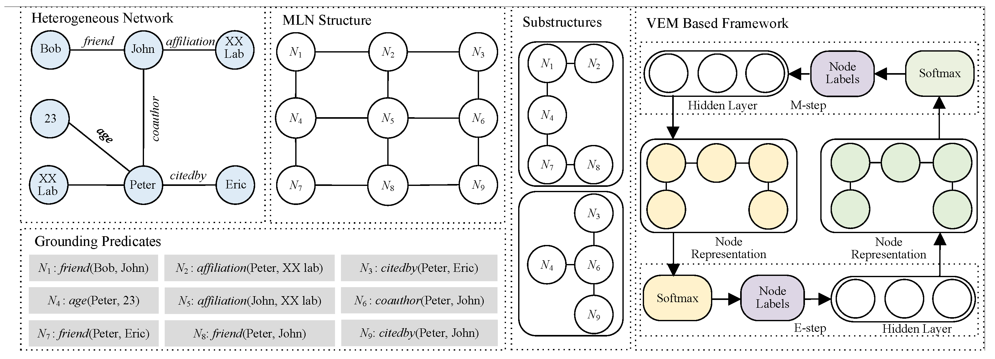
Multi-type relations could be encompassed into logical formulas for inter-dependency calculation. Markov logic networks (MLNs) offer an intuitive methodology for delineating network relationships through logical formulas, garnering increasing acclaim in the domain of multi-relational link prediction [9]. MLNs permit deviations from formulas with a penalizing mechanism rather than outright failure, which aligns with the inherent uncertainty prevalent in real-world relationships among entities. The magnitude of the penalty is regulated by weights assigned to individual formulas, with higher weights denoting a more robust endorsement of the associated patterns.

For instance, propositions such as “coauthors are likely to be friends” ($\mathit{coauthor}(x,y)\to \mathrm{friend}(x,y)$) and “if one author cites another, they might develop a friendly relationship” ($\mathit{citedby}(x,y)\to \mathrm{friend}(x,y)$) elucidate the interplay between different relations. By designing these formulas and employing grounding techniques, we can transform the information like $\mathit{citedby}(\mathrm{A},\mathrm{C})$ into grounded predicates, which serve as nodes in the MLN structure. The inter-dependency between different relations can be represented through the weights of formulas, which are calculated using MLN’s learning methods based on the values of MLN nodes. Similarly, the values of unknown nodes indicating link facts can be calculated through MLN’s inference methods using these learned weights.

In particular, LP in heterogeneous networks can be reformulated as an inference problem in MLNs and traditionally solved using Statistical Relational Learning (SRL) methods [10]. This approach predicts unknown links by inferring node labels in the MLN, using observed links as evidence, facing two major challenges for multi-relational LP: (1) the sparsity of observed links leads to numerous unobserved MLN nodes, and (2) the computational complexity of inference in large MLNs.

Traditional SRL inference methods for MLNs struggle with these challenges due to their inability to efficiently handle latent variables in sparse network settings. The variational expectation maximization (VEM) algorithm [10] addresses these limitations by introducing a principled framework for reasoning with latent variables. VEM enhances MLN inference for LP tasks in two key ways: first, by treating unobserved nodes as latent variables, it provides a systematic approach to handle network sparsity. Second, by approximating complex posterior distributions through variational inference, it significantly reduces the computational burden of exact inference in large-scale networks. Specifically, VEM iteratively updates variational and true posterior distributions to maximize the Evidence Lower Bound (ELBO) [11], thereby approximating the posterior distribution of node labels while maintaining computational tractability. This optimization process effectively balances inference accuracy with computational efficiency, making it particularly suitable for large heterogeneous networks.

To tackle the first challenge, we develop a substructure-based approach that iteratively partitions the MLN by selecting neighbors of unobserved nodes (seed nodes) corresponding to unknown links. The neighbor selection follows the 2-hop enclosing subgraph principle [12], balancing computational efficiency with prediction accuracy. Seed nodes are progressively selected based on VEM results from previous substructures, leading to an efficient MLN-based link prediction algorithm.

For the second challenge, we enhance the VEM framework by incorporating both neighboring node labels and MLN structural features. We leverage graph convolutional networks (GCNs) [13] to capture label dependencies and network topology. Specifically, we model the variational distribution of unobserved node labels as a categorical distribution and use GCNs to learn MLN structure representations, using neighboring node label distributions as feature matrices. This approach effectively captures the complex dependencies between different relationship types in the network.

Generally, the contributions of this paper are as follows:

• We introduce the concept of transforming multi-relational LP tasks into inferences in MLN, wherein LP is viewed as the estimation of node labels in MLN, with known links in a heterogeneous network considered as observed nodes in MLN.
• We propose a method to partition the MLN into distinct substructures to address the complexity of large MLN structures. Additionally, we present a VEM-based approach for calculating the distribution of node labels by incorporating formula features and the MLN structure.
• We define a termination condition for computing label distributions in MLN substructures and provide an algorithm for MLN-based LP.
• Extensive experiments demonstrate that our method surpasses both traditional and state-of-the-art (SOTA) approaches in terms of the accuracy of LP tasks.

The rest of this paper is organized as follows. We introduce related work, preliminaries, and the overview of our framework in Section 2. We elaborate our proposed inference framework of MLN for LP in Section 3. In Section 4, we report experimental results and performance studies. Lastly, we conclude and discuss future work in Section 5.

2. Related Work

In this section, we provide a comprehensive review of existing research on LP in both homogeneous and heterogeneous networks, along with an examination of inferences within MLN.

LP on homogeneous network. Heuristic and learning-based methods represent recent trends in LP research on homogeneous networks. Heuristic methods, such as utilizing common neighbors [14,15], are employed to infer link existence. Recent advancements in LP research have shown that learning-based methods like matrix factorization and network embedding techniques are more effective in acquiring node embeddings [16]. For instance, MHGCN+ [17] and HL-GNN [18] aggregate node embeddings through heterogeneous meta-path interaction and intra-layer propagation with inter-layer connections, respectively, to learn node embeddings. Moreover, ensemble methods [9,19] enhance LP tasks by combining the outcomes of heuristic and learning-based methods, leading to improved robustness at the expense of efficiency. These approaches construct classifier features through network embedding but struggle to achieve a unified representation of multiplex edges, prevalent in real-world heterogeneous network scenarios.

LP on heterogeneous network. Deep neural network-based methods have garnered significant attention for their adept feature extraction in LP tasks on heterogeneous networks [20,21]. These methods primarily focus on mining type-specific features to optimize prediction performance and subsequently combine relation embeddings through algebraic or transferable operations, as discussed in studies such as [7,8]. However, effectively capturing inter-dependencies among different types of links remains a challenge. Various techniques have been suggested to create link prediction models that minimize the loss associated with the representation of multi-type links. For instance, HRMNN [22] integrates a relational graph generator that leverages the topological attributes of heterogeneous graphs and combines object-level aggregation with a multi-head attention mechanism to produce more comprehensive node representations. MTTM [2] consists of a generative predictor and a discriminative classifier for link representations, enabling the discrimination of links and leveraging an adversarial neural network to maintain robustness against type differences. While these methods improve the representation of multiplex edges, challenges related to limited observed links and complex network architectures persist.

Researchers have endeavored to employ probabilistic graphical models (PGMs) to represent multi-type links in a unified manner, as discussed in [23]. First-order logic formulas have been utilized to model multi-relational databases with Bayesian network (BN), as outlined in [24], and the first-order BN serves as a statistical relational model capturing database frequencies.

As MLN formulas conclude predicates indicating various link types, inter-dependencies among various link types could be captured by the weights of formulas [25]. Meanwhile, MLN, acting as a PGM incorporating first-order logic rules, has been applied for representing relational data [26]. By converting heterogeneous networks into MLN and leveraging formulas, it enables a unified expression for multiplex edges. Nonetheless, optimization using SRL methods, as discussed in [27], is found to be non-scalable for LP tasks, primarily due to its inefficiency. Furthermore, the extensive structure of MLN leads to a vast search space and necessitates a costly inference process.

Inference in MLN. Efforts have been undertaken to enhance the efficiency and scalability of inferences in MLN for LP across diverse scenarios. For instance, QNMLN [25] expands on the formulas, while MCLA [28] refines its parameter updates for a range of practical tasks. The VEM algorithm [29] serves as the inference framework for MLN, with graph neural networks (GNNs) utilized in the E-step to capture the features of target relation nodes. ExpressGNN [30] utilizes GNN for node representation integration with formulas. On the other hand, PlogicNet [11] infers embeddings based on the local dependency of target nodes, yet overlooks their interactions. Pgat [26] optimizes the representations by employing graph attention neural network-based node embeddings. These methods use SRL to update parameters in the M-step by exploring the complete MLN, leading to challenges in generating precise embeddings for unlabeled nodes in efficient multi-relational LP. In contrast, our study in this paper utilizes GNNs to encapsulate the features of MLN and formulas in the M-step, and propose substituting the complete MLN with substructures to significantly decrease the search space of inferences.

3. Preliminaries

Consider a heterogeneous network with the following components: $\mathcal{V}$ represents the set of entities (e.g., papers, authors), $\mathcal{R}$ denotes the set of edges representing relationships, and $\mathcal{A}$ is the set of attributes associated with entities. We distinguish between observed and unobserved relationships where ${\mathcal{R}}_o$ represents the set of observed relations and ${\mathcal{R}}_u$ represents the set of unobserved relations.

Definition 1.

A heterogeneous network is defined as $H=(\mathcal{R},\mathcal{V}$, $\mathcal{A})$, where $\mathcal{R}$ = ${\mathcal{R}}_o\cup {\mathcal{R}}_u$ and $\left|\mathcal{R}\right|$+$\left|\mathcal{V}\right|$ > 2.

To transform our heterogeneous network into an MLN, we first represent relationships as logical predicates. Each relationship becomes a predicate $r(\mathit{x},\mathit{y})$, where r is a relation type from $\mathcal{R}$, and $\mathit{x}$ and $\mathit{y}$ are entities from $\mathcal{V}$.

These predicates form the building blocks of logical formulas that capture patterns in our data. When we ground these formulas (replace variables with actual entities), we create fact nodes in MLN. For example, in the academic citation network like in Figure 1a, we might observe that when author A cites both authors B and C, authors B and C are likely to be related. This pattern can be encoded as a logical formula: citedby (A, B) ∧ citedby (A, C) → citedby (B, C), in which $citedby$ (A, B), $citedby$ (A, C) and $citedby$ (A, B) become concrete nodes in MLN.

Let V represent all fact nodes in our MLN, consisting of $V_o$ and $V_u$, which denote the observed predicates (known relationships), and unobserved predicates (relationships to be inferred), respectively.

Definition 2.

An MLN is defined as $M=\left(G,\mathbf{w}\right)$, where the following are denoted:

• $G=\left(V,E\right)$ is an undirected graph where V is the set of fact nodes following Bernoulli distribution, E is the set of edges derived from logical formulas $\mathcal{F}$.
• The joint probability distribution over G is defined by

  $$P(V_o,V_u)={\displaystyle \frac{1}{Z\left(\mathbf{w}\right)}}exp\left(\sum _{f\in \mathcal{F}}{w}_f{n}_f(V_o,V_u)\right)$$
  where $Z\left(\mathbf{w}\right)$ is the partition function, $w_f$ is the weight of formula f, and $n_f(·)$ counts true groundings of f.

The parameters $\mathbf{w}$ of an MLN can be learned through discriminative learning by maximizing the pseudo-likelihood of $V_o$ [10]:

$$\underset{\mathbf{w}}{argmax}\sum _{n\in V_o}logp\left(y_n\right|MB\left(n\right))$$

(1)

where $y_n$ represents the label of node n, and MB(n) refers to the Markov blanket of n [31], encompassing its direct parents, direct children, and other parents of its direct children within the MLN.

The joint distribution $P\left(V_u\right)$ can be computed using maximum a posteriori (MAP) inference [26]:

$$\underset{n\in V_u}{argmax}\sum _{f\in F}{w}_f{n}_f(V_o,V_u)$$

(2)

In this paper, we aim to address the multi-relational LP task within G, by transforming H into G and calculating $P\left(V_u\right)$, where $V_u$ is corresponding to unknown links in H, and $P\left(V_u\right)$ represents the joint probability distribution. For the transformation, we firstly build G by establishing m formulas and the corresponding grounding. To address the efficiency bottleneck, we partition G into substructures $\left\{g^i\right|1\le i\le k\}$, where $V_u^i$ denotes the unobserved nodes in $g^i$. To calculate $P\left(V_u^i\right)$ efficiently, we propose the VEM-based inference method to update $\mathbf{w}$ by Equation (1) and calculate $P\left(V_u^i\right)$ by Equation (2) in each substructure $g^i$. Moreover, we introduce a termination condition to determine the necessity of computations in $g^{i+1}$. Consequently, we frame the inference of $P\left(V_u\right)$ into the computation of $P(V_u^1\mid g^1)$, $P(V_u^2\mid g^2)$, …, $P(V_u^k\mid g^k)$.

The key notations, abbreviations, and their descriptions are summarized in

Table 1. Notations and descriptions.

Notations	Descriptions
$H=(\mathcal{R},\mathcal{V},\mathcal{A})$	Heterogeneous network with entities $\mathcal{V}$, relations $\mathcal{R}$, and attributes $\mathcal{A}$
$G=\left(V,E\right)$	Graphical structure G with nodes V and links E
$\mathbf{w}$	Weight parameters of formulas
$M=\left(G,\mathbf{w}\right)$	MLN with distribution $P_{\mathbf{w}}$ with respect to parameters $\mathbf{w}$ over G
$Z\left(\mathbf{w}\right)$	Partition function with $\mathbf{w}$
$\mathcal{F}=\{f_i\mid 1\le i\le m\}$	Set of m formulas
$p\left(n\right)$	Label distribution of node n
$P\left(V\right)$	Joint distribution of node labels in V
$G=\left\{g^i\right|1\le i\le k\}$	Set of k MLN substructures
$N_2$	2-hop enclosing subgraph in H

and

Table 2. List of abbreviations.

Abbreviation	Full Term
LP	Link Prediction
MLN	Markov Logic Network
SRL	Statistical Relational Learning
VEM	Variational Expectation Maximization
ELBO	Evidence Lower Bound
GCN	Graph Convolutional Network

.

4. Proposed Method

The inference framework for efficient LP tasks is depicted in Figure 2, comprising the following three components.

• MLN substructure construction is proposed to construct MLN substructures to avoid the massive search space of the entire MLN, as presented in Section 4.1.
• VEM-based inference is proposed to calculate the joint distributions of nodes by extending the VEM with GCN, as presented in Section 4.2.
• MLN-based LP is proposed with the termination condition to fulfill LP by inferences in MLN, as presented in Section 4.3.

Figure 2. Overview of the proposed framework.

Figure 2. Overview of the proposed framework.

Our method initiates by transforming knowledge graph triples into grounded predicates to construct the MLN structure. Subsequently, we partition this MLN structure into coherent substructures. Finally, we apply VEM-based inference independently on each substructure, enabling efficient LP tasks on KGs.

4.1. MLN Substructure Construction

To compute the joint distribution $P\left(V_u\right)$ efficiently without navigating the extensive MLN search space, we divide G into k substructures, labeled as $G=\left\{g^i\right|1\le i\le k\}$. Constructing $g^i$ involves choosing unobserved nodes neighboring $V_o^{i-1}$ in $g^{i-1}$ (labeled as $V_u^i$) and progressively expanding through neighboring nodes in the MLN hop by hop, until adequate information is collected for label computation.

Viewed from a heterogeneous network perspective, the 2-hop enclosing subgraph $N_2(u,v)$ has been validated as containing adequate information for LP between entities u and v in the heterogeneous network H, with minimal approximation errors [12]. This validation guarantees the rationale to leverage the 2-hop enclosing subgraph principle for the expansive refinement of $V_u^{i-1}$ within G, which encompasses the links in H. To achieve this, we map $N_2(u,v)$ to corresponding fact nodes in MLN. Assuming that $N_2(u,v)$ includes $\eta$ predicates for facts like $coauthor(x,y)$, the analogous nodes in G to $N_2(u,v)$ in H are denoted as follows:

$$\begin{array}{cc}\hfill & {\mathcal{N}}^{\ast }\left(\mathfrak{r}(u,v)\right)=\hfill \\ \hfill & \{r_1(u,x),r_2(u,x),\cdots ,r_{\eta }(u,x)\}\hfill \\ \hfill & \cup \{r_1(v,x),r_2(v,x),\cdots ,r_{\eta }(v,x)\},\hfill \end{array}$$

(3)

where $\mathfrak{r}(u,v)$ is the MLN node corresponding to the link between u and v in H.

In the context of MLN, Equation (3) comprises ample information for the calculation of node labels for $\mathfrak{r}(u,v)$, guiding the exploration of $\mathfrak{r}(u,v)$’s neighbors through successive expansion hops. For convenience of expression, we use n and $N_h\left(n\right)$ to denote $\mathfrak{r}(u,v)$ and its neighbors in MLN, reached through h expansion hops, respectively. In particular, the expansion of the h-th hop is fulfilled by adding the neighbors of all the nodes in $N_{h-1}\left(n\right)$ iteratively. The expansion of $V_o^{i-1}$ halts when all generated neighbors encompass the nodes specified in Equation (3).

Note that without substructure construction, the interpretability of the entire MLN with respect to $\mathbf{w}$ can be calculated based on $P\left(V_u\right)$. While our approach partitions the computation process, the substructure construction is specifically designed for the efficient estimation of $P\left(V_u\right)$. Consequently, despite this division, the weights $\mathbf{w}$ can still be derived through conditional probability calculations, thus preserving the inherent interpretability of the original MLN.

By this procedure of substructure construction, we could transform $P\left(V_u\right)$ into $P(V_u^1\mid g^1)$, $P(V_u^2\mid g^2)$, …, $P(V_u^k\mid g^k)$ ($V_u^i\subset g^i$) with minimal approximation errors. Consequently, this partition strategy reduces computational complexity from $O\left(\right|E_{MLN}|·T)$ to $O\left({\sum }_{i=1}^k\right|E_g^i|·T_i)$, where ${\sum }_{i=1}^k|E_g^i|\ll |E_{MLN}|$ for typical sparse KGs. We summarize the steps of substructure construction in Algorithm 1 with time complexity $O(k·|V_g\left|\right)$, where $|V_g|$ denotes the average number of fact nodes in substructures.

4.2. VEM-Based Inference

In this section, we present a method to augment the VEM algorithm with GCNs to compute the labels of unobserved relation nodes.

4.2.1. Variational Distribution

To enhance LP efficiency in MLN, we propose computing the true posterior distribution $P\left(V_u\right|V_o)$ within the EM algorithm by treating the labels of $V_u$ as latent variables. Given the challenge posed by a large number of unobserved fact nodes in MLN for directly calculating $P\left(V_u\right|V_o)$, we approximate this distribution with a variational distribution $Q\left(V_u\right)$. Consequently, we derive $P\left(V_u\right|V_o)$ from $Q\left(V_u\right)$ by minimizing their KL divergence:

$$\begin{array}{cc}\hfill & KL(Q\left(V_u\right)\Vert P\left(V_u\right|V_o))\hfill \\ \hfill =& {\mathbb{E}}_Q[logQ\left(V_u\right)-logP\left(V_u\right|V_o)]\hfill \\ \hfill =& {\mathbb{E}}_Q[logQ\left(V_u\right)-log{\displaystyle \frac{P(V_u,V_o)}{P\left(V_o\right)}}]\hfill \\ \hfill =& {\mathbb{E}}_Q[logQ\left(V_u\right)-logP(V_u,V_o)]+logP\left(V_o\right),\hfill \end{array}$$

(4)

where ${\mathbb{E}}_Q[·]$ represents the expectation with respect to Q.

By swapping the term $logP\left(V_o\right)$ in Equation (4), we have

$$\begin{array}{cc}\hfill logP\left(V_o\right)=& KL(Q\left(V_u\right)\Vert P\left(V_u\right|V_o))\hfill \\ \hfill & -{\mathbb{E}}_Q[logQ\left(V_u\right)-logP(V_u,V_o)]\hfill \\ \hfill =& KL(Q\left(V_u\right)\Vert P\left(V_u\right|V_o))\hfill \\ \hfill & +{\mathbb{E}}_Q[logP(V_u,V_o)-logQ\left(V_u\right)].\hfill \end{array}$$

(5)

Algorithm 1 MLN Substructure Construction

Input:  observed nodes $V_o$, unobserved nodes $V_u$, MLN structure $G=(V,E)$, number of substructures k Output:  set of substructures $G^{\prime }=\{g^i\mid 1\le i\le k\}$ 1: $G^{\prime }\leftarrow \varnothing$ 2: $V_o^1\leftarrow V_o$ 3: for $i=1$ to k do 4:       $V_u^i\leftarrow V_u\cap {\bigcup }_{v\in V_o^i}{\mathcal{N}}_1\left(v\right)$ 5:       for each node n in $V_u^i$ do 6:             Obtain ${\mathcal{N}}^{\ast }\left(n\right)$ using Equation (3) 7:             $h\leftarrow 1$ 8:             while ${\mathcal{N}}^{\ast }\left(n\right)\not\subset {\mathcal{N}}_h\left(n\right)$ do // expansion 9:                   $h\leftarrow h+1$ 10:                 $NN\leftarrow \mathrm{neighbors}\mathrm{of}\mathrm{all}\mathrm{the}\mathrm{nodes}\mathrm{in}{\mathcal{N}}_{h-1}\left(n\right)$ 11:                 ${\mathcal{N}}_h\left(n\right)\leftarrow {\mathcal{N}}_{h-1}\left(n\right)\cup NN$ 12:             end while 13:             ${\mathcal{E}}_h\left(n\right)\leftarrow \mathrm{edges}\mathrm{w}.\mathrm{r}.\mathrm{t}.{\mathcal{N}}_h\left(n\right)$ in G 14:             $g^i\leftarrow ({\mathcal{N}}_h\left(n\right)\cup \left\{n\right\},{\mathcal{E}}_h\left(n\right))$ // the i-th substructure of G 15:       end for 16:       $V_o^i\leftarrow V_o^i\cup V_u^i$ // update observed nodes 17:       $G^{\prime }\leftarrow G^{\prime }\cup g^i$ // add substructure $g^i$ to $G^{\prime }$ 18: end for 19: return $G^{\prime }$

As $KL(Q\left(V_u\right)\Vert P\left(V_u\right|V_o))$ is non-negative, we define ${\mathbb{E}}_Q[logP(V_u,V_o)-logQ\left(V_u\right)]$ as the ELBO of $logP\left(V_o\right)$. Since $logP\left(V_o\right)$ is a constant with respect to $V_u$, we transform the minimization of $KL(Q\left(V_u\right)\Vert P\left(V_u\right|V_o))$ into the ELBO maximization by iterative executions of variational E-steps and M-steps.

4.2.2. Argumentation of VEM

Variational E-step. According to the mean-field theory [32], the variational distribution $Q\left(V_u\right)$ of all unobserved fact nodes is formed by the independent fact node $n(n\in V_u)$:

$$Q\left(V_u\right)=\prod _{n\in V_u}q\left(n\right).$$

(6)

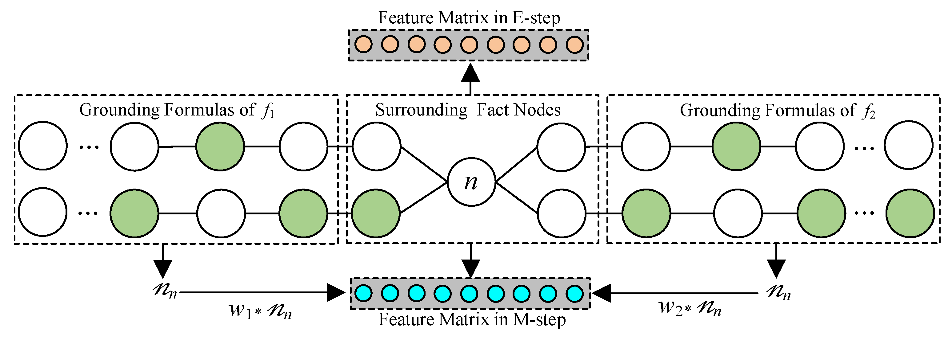
To calculate $q\left(n\right)$ in Equation (6), we adopt the GCN-based representation with Softmax function as the distribution of n. For this purpose, we take the labels of neighbors of n as the feature vector ${\mathcal{\mho }}_q^n$. The labels of the observed and unobserved fact nodes are 1 and 0, respectively. As shown in Figure 3, the labels of the fact nodes surrounding n form its feature vector. Thus, the feature matrix ${\mathbb{F}}_Q=\left[{\mathcal{\mho }}_q^n\right]$ could be constructed, and the distribution of n is

$$q\left(n\right)=Cat\left(y_n\right|Softmax\left(\mathbb{A}{\mathbb{F}}_Q{\mathbb{W}}_Q\right)),$$

(7)

where Cat denotes the categorical distribution, $\mathbb{A}$ is the adjacency matrix corresponding to the graph structure, and ${\mathbb{W}}_Q$ is the weight matrix. Since ${\mathbb{W}}_Q$ could be optimized by observed nodes, we divide the optimization of ${\mathbb{W}}_Q$ into the following two parts:

• For unobserved fact nodes $V_u$, we update ${\mathbb{W}}_Q$ by maximizing

  $${\mathcal{L}}_u=-\sum _{n\in V_u}KL(Q^{\prime }\left(V_u\right)\Vert Q\left(V_u\right)),$$

  (8)

  where $Q^{\prime }\left(V_u\right)$ is the distribution of unobserved fact nodes in the previous iteration round. Since both unobserved and observed fact nodes follow the same distribution, we initialize $P\left(V_o\right)$ to $Q^{\prime }\left(V_u\right)$ in the first round of iteration.
• For the observed fact nodes $V_o$, we use the cross-entropy loss to make the GCN fit the true labels:

  $${\mathcal{L}}_o=-\sum _{n\in V_o}{y}_{n}log{p}_c\left(y_n\right),$$

  (9)

  where $y_n$ is the label of n in $V_o$, and $p_c\left(y_n\right)$ is the probability that n is predicted as true.

Thus, we sum Equations (8) and (9) as the following training loss of GCN to obtain the variational distribution $Q\left(V_u\right)$:

$${\mathcal{L}}_Q={\mathcal{L}}_u+{\mathcal{L}}_o.$$

(10)

M-step. To maximize the expectation of $logP(V_u$, $V_o)$, we use a similar method as Equation (6) to formulate $P\left(V_u\right)={\prod }_{n\in V_u}p\left(v\right)$. Then, we leverage another GCN to obtain the node representations for categorical distribution:

$$p\left(n\right)=Cat\left(y_n\right|Softmax\left(\mathbb{A}{\mathbb{F}}_P{\mathbb{W}}_P\right)).$$

(11)

Due to the same structure of these two GCNs in the same iteration round, the adjacency matrix $\mathbb{A}$ in Equation (11) is the same with that in Equation (7). An element in ${\mathbb{F}}_P$ represents the feature vector ${\mathcal{\mho }}_p^n$ of n in $V_u$ and the value of ${\mathcal{\mho }}_P^n$ is determined by the m formulas and corresponding weights $\mathbf{w}$. Let ${\mathfrak{n}}_n$ denote the number of truth-value nodes linked with each formula $f_j$, respectively. Let $w_j$ be the weight of $f_j$. Then, we multiply the weight and number of truth-value nodes to achieve the feature ${\mathcal{\mho }}_p^n=[w_j\ast {\mathfrak{n}}_n]$. As shown in Figure 3, we construct the feature matrix ${\mathbb{F}}_p$ in the M-step by the numbers of nodes in grounding formulas of $f_1$ and $f_2$, as well as their weights $w_1$ and $w_2$.

Let $\mathfrak{n}\left(o\right)$ and $\mathfrak{n}\left(Q\left(V_u\right)\right)$ be the real and expected numbers of true groundings of formulas, respectively. We use their difference as the gradient of $\mathbf{w}$ with the previous iteration round:

$${\nabla }_{\mathbf{w}}{\mathbb{E}}_Q[logP\left(V_u\right)]=\mathfrak{n}\left(o\right)-\mathfrak{n}\left(Q\left(V_u\right)\right),$$

(12)

where $Q\left(V_u\right)$ is the joint distribution of $V_u$ calculated by the E-step in the previous iteration round.

Additionally, if the fact node is not grounded from any predicate in the j-th formula (i.e., the node is not linked to this formula), we set the corresponding weight $w_j$ to 0.

Then, we design the following predicate loss to update ${\mathbb{W}}_p$ by maximizing ${\mathbb{E}}_{Q}logP(V_u,V_o)$:

$${\mathcal{L}}_P=-\sum _{n\in V_u,V_o}logp\left(y_n\right),$$

(13)

where $y_n(y_n\sim Q\left(V_u\right))$ is the label of n.

Thus, ${\mathbb{E}}_{Q}logP(V_u,V_o)$ could be maximized by the optimal ${\mathbb{W}}_P$ in the current iteration, and the distribution $P\left(V_u\right|V_o)$ of unobserved fact nodes could be approximated efficiently.

4.2.3. Inference Algorithm

To calculate the joint distribution of fact nodes in each substructure, we use the VEM-based inference to update the parameters of GCNs in the variational E-steps and M-steps given the observed fact nodes.

We first initialize $\mathbf{w}$ with a normal distribution for training ${\mathbb{W}}_P$ with $V_o^i$ in the M-step. Then, in the variational E-step, we optimize the variational distribution $Q\left(V_u^i\right)$ with the output $P\left(V_u^i\right|V_o^i)$. In the M-step, we optimize the posterior distribution $P\left(V_u^i\right|V_o^i)$ with $Q\left(V_u^i\right)$ calculated by Equation (7). Then, we alternatively optimize $Q\left(V_u^i\right)$ and $P\left(V_u^i\right|V_o^i)$ until their KL divergence is less than the given threshold or the given maximal iteration number is reached.

We summarize the above ideas in Algorithm 2. In the worst case, the time complexity is $O(T_1·|E_{g^i}|·\mathcal{L})$, where $T_1$ is the maximal iteration number of steps 7∼13, $|E_{g^i}|$ is the average number of edges in each substructure, and $\mathcal{L}$ is the number of layers in GCN.

Algorithm 2 VEM-based inference

Input:  the threshold $\varrho$ of KL divergence, the MLN substructure $g^i$, the observed fact nodes $V_o^i$, the weights $\mathbf{w}$, the unobserved fact nodes $V_u^i$ Output:  posterior distribution $p\left(V_u^i\right|V_o^i)$ 1: Initialize $\mathbf{w}$ and ${\mathbb{W}}_P$ 2: Obtain ${\mathbb{F}}_P$ with $V_o^i$ by Equation (12) 3: Obtain $\mathbb{A}$ by edges of $g^i$ 4: Optimize ${\mathbb{W}}_P$ by Equation (13) 5: $p\left(V_u^i\right|V_o^i)\leftarrow Softmax\left(\mathbb{A}{\mathbb{F}}_P{\mathbb{W}}_P\right)$ // by Equation (11) 6: $j\leftarrow 1$ 7: while $KL\left(p\right(V_u^i\mid {\mathbb{W}}_P)\Vert Q(V_u^i\mid {\mathbb{W}}_q))\ge \varrho$ do 8:       Update ${\mathbb{W}}_Q$ in E-step by Equation (10) 9:       Optimize $Q\left(V_u^i\right)$ by Equation (7) 10:     Update ${\mathbb{W}}_P$ in M-step by Equation (13) 11:     Optimize $P\left(V_u^i\right|V_o^i)$ by Equation (11) 12:     $j\leftarrow j+1$ 13: end while 14: $T_1\leftarrow j-1$ 15: return $P\left(V_u^i\right|V_o^i)$

4.3. MLN-Based LP

The labels of fact nodes in $g^i$ could be determined through logical inference based on formulas rather than the VEM inference method. For instance, a grounding formula with a non-zero weight such as $\mathit{citedby}(\mathrm{A},\mathrm{B})\cap \mathit{citedby}(\mathrm{A},\mathrm{C})\to \mathit{citedby}(\mathrm{B},\mathrm{C})$ can create a true relation-node $\mathit{citedby}(\mathrm{B}$, $\mathrm{C})$ if both $\mathit{citedby}(\mathrm{A},\mathrm{B})$ and $\mathit{citedby}(\mathrm{A},\mathrm{C})$ hold. By iteratively obtaining the joint distribution of unobserved node labels using Algorithm 2 based on the observed fact nodes in the substructures, more observed nodes can be acquired. A comparison with the joint distribution derived from logical formulas reveals an increasing discrepancy in VEM-based inferences as more unobserved fact nodes are updated to observed. Consequently, we opt to halt the iterative inferences when the difference surpasses a specified threshold, enabling the calculation of the joint distribution of $V_u$ for LP tasks.

Without loss of generality, we establish the KL divergence-based termination condition to determine whether further calculation should proceed by measuring the difference between the distribution of fact node labels obtained through logical evaluation and VEM-based methods:

$$KL\left(P_{\mathfrak{f}}\left(U\right|V_o^i)\right|P_{\mathfrak{e}}\left(U\right|V_o^i)).$$

(14)

Here, $V_o^i$ denotes the observed fact nodes in $g^i$, U represents the sole unobserved node in each formula, which can be evaluated logically as 1 or 0, corresponding to true or false, respectively. $P_{\mathfrak{f}}$ signifies the value of U given $V_o^i$ through logical evaluation, while $P_{\mathfrak{e}}$ denotes the joint distribution from VEM-based inferences. A smaller KL divergence indicates that the two joint distributions calculated by VEM-based inferences and logical evaluations are more consistent.

To calculate $P_{\mathfrak{f}}\left(U\right|V_o^i)$, we utilize Equation (12) to compute ${\mathbf{w}}^i$, deriving the nonzero-weight formulas ${\mathcal{F}}^i$ (${\mathcal{F}}^i\subset \mathcal{F}$). Subsequently, we construct U using the fact nodes, whose labels could be logically inferred as true by ${\mathcal{F}}^i$. Therefore, $P_{\mathfrak{f}}\left(U\right|V_o^i)$ could be redefined as $P_{\mathfrak{f}}\left(U\right|V_o^i,{\mathcal{F}}^i)$. As $P_{\mathfrak{e}}\left(U\right|V_o^i)$ could be calculated using Algorithm 2 as ${\displaystyle \sum _{n\in U}}{p}_{\mathfrak{e}}\left(n\right)$, we transform Equation (14) into

$$\begin{array}{cc}\hfill & KL\left(P_{\mathfrak{f}}\left(U\right|V_o^i)\right|P_{\mathfrak{e}}\left(U\right|V_o^i))\hfill \\ \hfill =& KL\left(P_{\mathfrak{f}}\left(U\right|V_o^i,{\mathcal{F}}^i)\right|\sum _{n\in U}{P}_{\mathfrak{e}}\left(n\right))\hfill \\ \hfill =& \sum _{n,n^{\prime }\in U,n^{\prime }\ne n}{p}_{\mathfrak{f}}\left(n\right)log\left[{\displaystyle \frac{p_{\mathfrak{f}}\left(n\right)}{p_{\mathfrak{e}}\left(n^{\prime }\right)}}\right].\hfill \end{array}$$

(15)

Equation (15) serves as the termination criterion, indicating that if it falls below a specified threshold, the computation in $g^{i+1}$ continues. By this pause mechanism, we could prevent noisy data from causing significant error impacts. These concepts are consolidated in Algorithm 3. Within each substructure $g^i(1\le i\le k)$, the time complexity of step 4 is $O\left(\right|V_{g^i}\left|\right)$, where $|V_{g^i}|$ denotes the average number of nodes in $g^i$. Step 5’s time complexity is $O(T_1·\mathcal{L}·|E_{g^i}|)$ as per Algorithm 2, with $|E_{g^i}|$ representing the average edge count in $g^i$. The time complexity of steps 6 through 7 is $O\left(\right|V_{g^i}|$). Hence, in a scenario where $T_2$ substructures are constructed, the time complexity of Algorithm 3 amounts to $O(T_2·\left(\right|V_{g^i}|+T_1·\mathcal{L}·|E_{g^i}\left|\right))$, where $|E_{g^i}|$ and $|V_{g^i}|$ are considerably smaller than $\left|E\right|$ and $\left|V\right|$, respectively. Specifically, the time complexity of substructure construction is $O(T_2·|V_{g^i}\left|\right)$, while the VEM-GCN integration exhibits a time complexity of $O(T_2·T_1·\mathcal{L}·|E_{g^i}\left|\right)$, respectively.

Algorithm 3 MLN-based LP

Input:  the set of initial observed fact nodes $V_o$, the set of formulas $\mathcal{F}$, the threshold $\tau$ of KL divergence between $P_{\mathfrak{f}}$ and $P_{\mathfrak{e}}$ Output:  joint distribution $P\left(V_u^{\prime }\right)$ 1: $V_u^{\prime }\leftarrow \varnothing$ 2: $i\leftarrow 1$ 3: while $KL(P_{\mathfrak{f}}\left(U\right|V_o^i,{\mathcal{F}}^i)\parallel P_{\mathfrak{e}}\left(U\right|V_o^i))\le \tau$ do 4:       Obtain $g_i,V_u^i,V_o^i$ with $V_o$ by Algorithm 1 5:       Obtain $P\left(V_u^i\right|V_o^i)$ by Algorithm 2 6:       Obtain ${\mathcal{F}}^i$ with ${\mathbf{w}}^i$ by Equation (12) 7:       Obtain U via ${\mathcal{F}}^i$ by logical way 8:       $V_u^{\prime }\leftarrow V_u^{\prime }\cup V_u^i$ 9:       $i\leftarrow i+1$ 10: end while 11: $T_2\leftarrow i-1$ 12: return $P\left(V_u^{\prime }\right)$

5. Experiments

Our proposed method is evaluated based on the following inquiries:

• Comparing the accuracy of our method for multi-relational LP tasks with that of competitors.
• Assessing how our VEM-based inference method enhances the efficiency of MLN-based LP.
• Investigating the impact of parameters on the accuracy of the LP.

5.1. Experiment Settings

Datasets. Our experiments were carried out on five heterogeneous networks: the academic network, Aminer; the network of relatives, Kinship [30]; the medical relation network, UMLS [11]; the word net WN18RR [29]; and the social knowledge base Freebase15k-237 [33]. The dataset statistics are presented in

Table 3. Statistics of datasets.

Dataset	#Entity	#Relation Type	#Relation
FB15k-237	14,541	237	592,213
WN18RR	40,943	11	93,003
Aminer	3,804,789	2	8,024,869
Kinship	104	25	10,686
UMLS	135	46	6529

.

Formulas. Logical formulas for multi-relational LP tasks were devised for each dataset and translated into inferences within MLN. Specific formulas for each dataset are delineated in

Table 4. Formulas.

Dataset	Formulas
Aminer	FieldinA (x, y) ⟶ Citedby (x, y) AffiliationinA (x, y) ⟶ Coauthor (x, y) FieldinA (x, y) ⟶ Citedby (x, y) (Coauthor (x, y) ∧ Coauthor (y, z)) ⟶ Coauthor (x, z) (Citedby (x, y) ∧ Citedby (y, z)) ⟶ Citedby (x, z)
UMLS	Affects (x, y) ∧ Affects (y,z) ∧ Affects (x, z) Affects (x, y) ∧ Causes (x, y)
Kinship	Father (x, y) ∧ Male(x) ∧ Son (x, y) Mother (x, y) ∧ Male(x) ∧ Son (x, y) Father (x, y) ∧ Father (x, z) ∧ Male(y) ∧ Male(z) ∧ Brother (y, z)
FB15k-237	Position (x, y) ∧ Position (y, z) ⟶ Position (x, z) Ceremony (x, y) ∧ Ceremony (y, z) ⟶ CategoryOf (x, z) Film (x, y) ∧ Film (y, z) ⟶ Participant (x, z) StoryBy (x, y) ⟶ Participant (x, y) Adjoins (x, y) ∧ Country (y, z) ⟶ ServiceLocation (x, z)
WN18RR	Member_eronym (x, y) ∧ Hypernym (x, y) Similar_to (x, y) ∧ Derivationally_related_form (x, y)

.

Comparison methods. We compared two types of methods: deep learning-based methods including SEAL [12] and Matrix Factorization (MF) [16], and MLN-based methods including ExpressGNN [30], PlogicNet [11], Pgat [26], RNNlogic [29], and MLN [10]. The latter category employs MLN to model heterogeneous networks, facilitating learning and inferences for diverse downstream tasks. They are summarized as follows:

• SEAL adopts GNN for node representation by learning the structural information.
• MF transforms the representation matrix into multiplication of matrices to enhance node representation.
• ExpressGNN uses a GNN variant to conduct the variational inference in MLN structures.
• PlogicNet uses GNN to embed the graphical structures and incorporates the weights of formulas by VEM.
• Pgat incorporates graph attention network embeddings to infer the relations.
• RNNlogic leverages recurrent neural networks to generate high-quality formulas for inferences in MLN.
• MLN uses SRL-based methods to generate posterior distributions of nodes in MLN.

Implementation. We utilized accuracy to evaluate the efficacy of our proposed method, defined as the ratio of correct predictions generated by the LP methods. Efficiency was assessed through execution time, encompassing the overall time for parameter updates and link predictions.

For the learning-based methods, we treated the evidence nodes in MLN and their labels as the training and test sets, respectively. To execute multi-relational LP using MLN, we formulated the MLN structure for each dataset. In the case of the Aminer dataset, we randomly selected subsets by varying the sizes from 10,000, 5000, 2000, to 1000 individuals. SEAL and MF were applied to the datasets for each link type, with the average accuracy serving as the LP outcome. For robust evaluation, we repeated each experiment 5 times with different random seeds and reported the mean performance along with standard deviation. For each experimental configuration, the training and testing processes were executed independently, maintaining consistent hyperparameter settings across all runs to ensure fairness.

Our experiments were conducted on a machine equipped with a 6000Ada GPU, 128 GB of memory, and an i9-9900K CPU. All implementations were carried out using Python 3.7. We primarily used PyTorch v1.12.1 and ProbCoG libraries.

5.2. Experimental Results

Accuracy. We assessed the efficacy of our method by comparing its accuracy with various other methods. To ensure fairness in the experiments, we maintained consistent links in the test set. For discerning accuracy across different scales, we segmented the Aminer dataset into subsets: Aminer-10000, Aminer-5000, Aminer-2000, and Aminer-1000, containing 12,601, 3591, 2384, and 1189 relations, respectively. Two types of links were designated for prediction, with an 8/2 ratio between training and testing data. Furthermore, we examined the outcomes of combinations with varying numbers of link types and ratios, specifically (3 types, 8/2) and (2 types, 7/3), to analyze the impact of these factors on results. The accuracy comparisons are detailed and summarized in

Table 5. Accuracy with 2-type links and ratio 8/2 with statistical analysis.

Method	Kinship	UMLS	WN18RR	FB15k-237	Aminer-10,000	Aminer-5000	Aminer-2000	Aminer-1000
SEAL	85.86	83.22	15.29	14.33	70.44	86.34	82.88	77.43
MF	72.41	82.37	-	-	66.42	64.77	79.88	70.55
ExpressGNN	91.88	86.91	-	40.7	80.31	89.46	78	87.88
MLN	92.22	85.32	-	-	-	-	82	81.56
PlogicNet	85.33	84.9	39.8	23.7	68.3	72.21	76.91	84.32
Pgat	88.31	80.2	39.5	37.7	72.45	62.83	80.5	82.21
RNNlogic	61.67	72.21	44.6	24.5	58.93	66.67	72.12	65.01
Ours	94.87	87.33	42.2	45.4	83.32	92.31	87.32	89.5
p-value	0.027 *	0.780	0.255	0.042 *	0.060	0.029 *	0.009 **	0.248
95% CI	[92.52, 97.22]	[84.39, 90.27]	[38.08, 46.32]	[40.89, 49.91]	[80.18, 86.46]	[89.76, 94.86]	[83.99, 90.65]	[86.76, 92.24]

Note: The highest accuracy is indicated in bold. * p < 0.05, ** p < 0.01. CI = Confidence Interval. p-values show a comparison of our method against the best competitor.

,

Table 6. Accuracy with 3-type of links and ratio 8/2 with statistical analysis.

Method	Kinship	UMLS	WN18RR	FB15k-237	Aminer-10,000	Aminer-5000	Aminer-2000	Aminer-1000
SEAL	80.21	74.12	13.29	11.85	68.13	81.66	79.15	75.22
MF	61.33	76.28	-	-	62.77	61.39	75.49	68.17
ExpressGNN	90.42	84.18	-	38.27	73.11	85.33	73.91	83.39
MLN	80.19	79.41	-	-	-	-	75.11	76.48
PlogicNet	79.44	79.27	33.6	20.36	65.29	65.49	73.81	80.09
Pgat	86.22	76.12	34.5	31.11	69.35	55.19	75.05	73.81
RNNlogic	55.71	69.18	39.6	20.75	53.16	63.29	66.74	63.55
Ours	92.92	82.33	39.7	42.4	78.15	87.47	83.22	85.65
p-value	0.033 *	0.041 *	0.892	0.019 *	0.048 *	0.037 *	0.022 *	0.175
95% CI	[90.47, 95.37]	[79.20, 85.46]	[36.18, 43.22]	[38.63, 46.17]	[74.89, 81.41]	[84.74, 90.20]	[80.07, 86.37]	[82.51, 88.79]

Note: The highest accuracy is indicated in bold. * p < 0.05. CI = Confidence Interval. p-values show a comparison of our method against the best competitor.

and

Table 7. Accuracy with 2-type links and ratio 7/3 with statistical analysis.

Method	Kinship	UMLS	WN18RR	FB15k-237	Aminer-10,000	Aminer-5000	Aminer-2000	Aminer-1000
SEAL	81.14	77.5	9.55	9.93	63.21	85.17	76.91	70.66
MF	66.15	73.98	-	-	60.29	62.18	71.53	60.4
ExpressGNN	82.19	82.17	-	34.44	70.81	85.12	74.21	82.02
MLN	81.72	79.02	-	-	-	-	73.29	73.19
PlogicNet	79.17	76.79	29.18	19.74	61.39	68.91	71.59	72.91
Pgat	69.11	72.72	36.97	33.28	66.75	54.71	62.15	58.44
RNNlogic	50.06	63.55	41.91	23.19	52.13	61.28	62.51	65.01
Ours	89.46	82.11	39.4	41.41	74.91	85.19	82.04	81.66
p-value	0.001 **	0.949	0.202	0.015 *	0.044 *	0.957	0.003 **	0.818
95% CI	[86.84, 92.08]	[78.93, 85.29]	[35.66, 43.14]	[37.52, 45.30]	[71.53, 78.29]	[82.46, 87.92]	[78.75, 85.33]	[78.34, 84.98]

Note: The highest accuracy is indicated in bold. * p < 0.05, ** p < 0.01. CI = Confidence Interval. p-values show a comparison of our method against the best competitor.

. In cases where a model failed to operate due to memory constraints, this is denoted by `-’. Our findings suggest the following:

• Across 2-type and 3-type links at different train–test ratios, our method attains an average accuracy of 94.87%, which stands as the highest accuracy across all dataset sizes. Notably, our method enhances accuracy by approximately 3.7%, 2.9%, 0.5%, 6.0%, and 11.5% compared to the highest accuracy achieved by the comparison methods, respectively.
• Across varying sizes of the Aminer datasets, our method consistently surpasses all competitors, showcasing enhanced robustness. Notably, our method boosts accuracy by 3.7%, 3.1%, 5.3%, and 1.8% compared to the second-highest performing model on Aminer with 10,000, 5000, 2000, and 1000 individuals, respectively.
• The MLN-based methods (ExpressGNN, MLN, PlogicNet, Pgat, RNNlogic, and our method) attain average accuracies of 85.71%, 82.81%, 41.52%, 34.4%, and 72.66% on the Aminer, Kinship, UMLS, WN18RR, and FB15k-237 datasets, respectively, surpassing the learning-based methods (SEAL and MF) by 8.3%, 0.1%, 171.55%, 140.1%, and 6.2%, respectively. Our method achieves accuracies of 72.66%, 76.7%, 79.48%, and 81.75%, outperforming the second-highest model by an average of 3.65% on the Aminer datasets with 10,000, 5000, 2000, and 1000 individuals, respectively.

Also, we conducted experiments on different missing link ratios to evaluate the robustness of our method. We randomly removed 10%, 30%, and 50% of the Kinship, UMLS, WN18RR, and FB15k-237 datasets, respectively, and various sizes of Aminer. The accuracy comparisons are detailed in

Table 8. Accuracy under various missing link ratios.

Dataset	Edge Removal
	10 (%)	30 (%)	50 (%)
Kinship	91.12	83.48	71.15
UMLS	84.28	77.72	67.24
WN18RR	40.09	35.87	29.54
FB15k-237	42.68	36.32	29.51
Aminer-10000	79.99	72.49	61.66
Aminer-5000	88.62	80.31	68.31
Aminer-2000	83.82	75.97	64.62
Aminer-1000	85.92	77.87	66.33

. Our findings suggest the following:

• When 10% of the edges are removed, the performance of the model shows a slight overall decline, with more pronounced decreases in the sparse datasets such as WN18RR and FB15k-237, reaching 5% and 6%, respectively. In other datasets, the performance degradation is relatively smaller, approximately 3.5–4%.
• As the edge removal increases to 30%, performance degradation becomes more significant. The FB15k-237 dataset is most affected, with a 20% reduction, while WN18RR shows a 15% decrease. Kinship, UMLS, and the Aminer series datasets experience reductions between 11 and 13%.
• When 50% of edges are removed, all datasets undergo substantial performance deterioration. The FB15k-237 dataset remains the most severely impacted, with a 35% decrease; WN18RR declines by 30%; Kinship decreases by 25%; UMLS exhibits the smallest relative reduction at 23%; and all Aminer series datasets uniformly experience a 26% decrease.
• Overall, sparser graph structures (e.g., WN18RR and FB15k-237) demonstrate higher sensitivity to edge removal, whereas denser relationship graphs (e.g., UMLS and Kinship) display better robustness. The Aminer series datasets, regardless of size, show similar patterns of performance degradation.

The accuracy enhancements observed in multi-relational LP validate the efficacy and robustness of our method through the integration of the VEM-based inference framework.

Efficiency. Efficiency evaluation of our method involved comparing its execution time with various MLN-based methods in multi-relational LP on the benchmarks WN18RR, FB15k-237, and Aminer datasets. The total execution time (TT), time for the E-step (ToE), and time for the M-step (ToM) are illustrated in Figure 4. It is noteworthy that the execution times of MLN and NMLN are not included due to their significantly longer durations compared to the listed methods. Our observations reveal the following:

• On WN18RR and FB15k-237 datasets, each containing over 10,000 entities, our method demonstrates the shortest processing time and surpasses the second-fastest model by an average of 42.37%.
• When compared to pgat, RNNlogic, ExpressGNN, and PlogicNet on FB15k-237, our method reduces the total execution time (TT) by 40%, 56.82%, 63.3%, and 69.7%, respectively. On WN18RR, our method outperforms pgat, RNNlogic, ExpressGNN, and PlogicNet by 19.09%, 42.86%, 49.14%, and 55.5%, respectively.
• In terms of the E-step (ToE) and M-step (ToM), our method achieves average improvements of 57.85% and 21.15% on WN18RR, and 71.96% and 37.41% on FB15k-237, respectively.

These results illustrated in Figure 4 denote that our method demonstrates efficiency advancements on TT, ToE, and ToM, on the datasets with more than 10,000 entities.

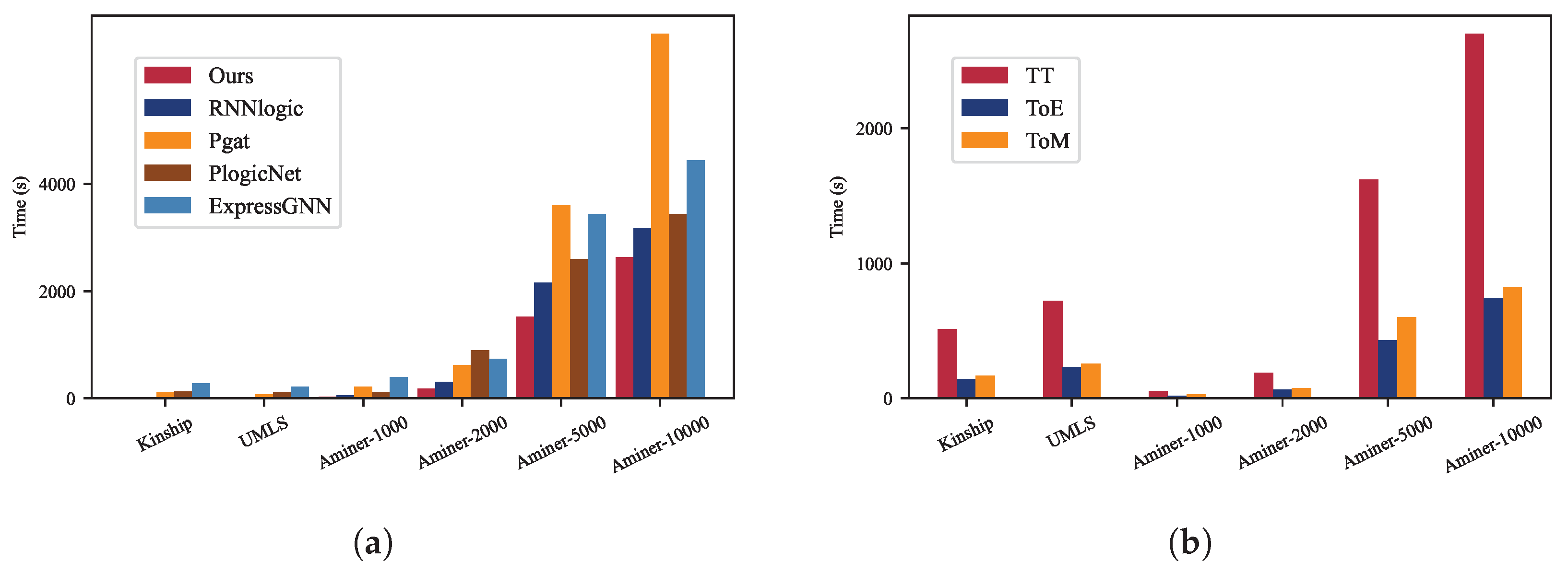
Moreover, to assess efficiency across datasets of different sizes, we compared the total execution time (TT) on UMLS, Kinship, Aminer-10000, Aminer-5000, Aminer-2000, and Aminer-1000, each comprising fewer than 10,000 entities, as depicted in Figure 5a. Furthermore, Figure 5b presents the TT, time for the E-step (ToE), and time for the M-step (ToM) of our method, showcasing the execution durations of these steps across various dataset sizes. Our analysis indicates the following:

• As depicted in Figure 5a, our method exhibits the shortest total execution time among the datasets containing fewer than 10,000 entities, surpassing RNNlogic, Pgat, and PlogicNet. On average, our model consumes 33.2% less time than the second-fastest model in each dataset.
• As illustrated in Figure 5b, the execution time for the M-step (ToM) in our method averages 26% more than that for the E-step (ToE) across different datasets. Furthermore, the total time (TT) of our model demonstrates exponential growth with increasing data size, whereas both ToE and ToM exhibit nearly linear growth.

Impacts of parameters. We assessed the influence of experimental variables on the efficacy of LP by examining the accuracy of different methods while altering the number of formulas on Aminer-10000, FB15k-237, and Kinship datasets with more than 3 formulas, as detailed in

Table 9. Accuracy of LP with various numbers (3, 4, 5) of logical formulas with statistical analysis.

Methods	Aminer-10000			FB15k-237			Kinship
	3	4	5	3	4	5	3	4	5
ExpressGNN	70.43	76.21	80.31	35.43	38.71	40.7	86.43	87.42	91.88
Pgat	65.12	67.31	72.45	15.12	17.31	23.7	75.12	83.21	85.33
PlogicNet	60.44	67.12	68.3	35.44	36.12	37.7	86.44	88.31	87.12
Ours	78.32	81.44	83.32	42.32	45.44	45.4	88.32	91.44	94.87
p-value	0.018 *	0.039 *	0.060	0.012 *	0.008 **	0.042 *	0.037 *	0.019 *	0.027 *
Improvement	7.89%	5.23%	3.01%	6.89%	6.73%	4.70%	1.89%	3.13%	2.99%
95% CI	[75.6, 81.0]	[78.9, 84.0]	[80.2, 86.4]	[39.8, 44.9]	[42.7, 48.2]	[42.5, 48.3]	[85.7, 91.0]	[88.5, 94.4]	[92.5, 97.2]

Note: The highest accuracy is indicated in bold. * p < 0.05, ** p < 0.01. CI = Confidence Interval for our method.

. Our analysis indicates that:

• Our method attains average accuracies of 81.03%, 91.54%, and 44.39% on Aminer-10000, FB15k-237, and Kinship, respectively, surpassing the second-best competitors by 3.75%, 2.87%, and 11.55% on average. This underscores the robustness of our approach.
• Accuracy shows a slight increment with an increase in logical formulas, suggesting that more formulas lead to improved accuracy. Conversely, a higher number of formulas results in a substantially larger grounded MLN structure, introducing more unlabeled nodes in MLN that could potentially impact accuracy negatively. Notably, as depicted in Table 9, the accuracy on PlogicNet decreases by an average of 1.34% with the increase in formulas.

Ablation study. We conducted ablation experiments on the distinct contributions of each component in our proposed framework, the results of which are shown in

Table 10. Accuracy of LP with different model configurations.

MLN	SRL	VEM	GCN	SC	TC	FB15k	WN18RR	Aminer	Kinship	UMLS
✓	✓					-	-	0.68	0.76	0.79
✓		✓	✓			0.74	0.85	0.81	0.87	0.91
✓		✓	✓	✓		0.72	0.83	0.79	0.85	0.89
✓		✓	✓	✓	✓	0.78	0.88	0.83	0.89	0.94

. The base MLN with SRL establishes a foundation but shows limitations on larger, complex datasets like FB15k and WN18RR. The VEM-GCN integration substantially enhances performance with a 7–12% across all datasets. Substructure condition (SC) presents an intriguing efficiency–accuracy trade-off. While moderately impacting accuracy with a reduction of only 1–2%, SC substantially enhances computational efficiency, delivering processing speeds up to 3.5x faster on larger datasets. Most significantly, the termination condition (TC) mechanism provides the most substantial accuracy gains, boosting performance by 4–6% when combined with SC across all datasets. The optimal configuration with all components except SRL achieves the highest accuracy.

In conclusion, based on the diverse experimental conditions and datasets examined, our method demonstrates the highest average accuracy in multi-relational LP across various datasets and link types, surpassing competitors by over 30% in efficiency.

6. Conclusions

First, we establish a perspective by transforming multi-relational LP into a node label estimation problem within MLN, treating known links as observed nodes. This transformation provides a principled probabilistic foundation for handling the inherent complexity of heterogeneous networks. Second, our substructure construction method partitions significantly enhance computational efficiency while preserving semantic relationships. Complementing this, our VEM-based framework strikes a balance between precision and computational feasibility. Third, the proposed terminating computation ensures both accuracy and efficiency in practical applications, making our approach viable for real-world heterogeneous networks. Finally, the experimental results demonstrate our method’s advantages in terms of efficiency, robustness, and accuracy. In all, our approach indeed bridges the critical gap between unknown links in heterogeneous networks and unobserved nodes in MLN, establishing a hybrid approach to link prediction that combines the strengths of both machine learning techniques and logical deduction.

Efficient inferences heavily depend on the MLN structure size, shaped by the formulated formulas for diverse multi-relational LP tasks. In future research, we aim to explore automatic formula selection to strike a balance between efficiency and efficacy. Furthermore, the combined VEM-GCN architecture possesses robust capacity for capturing temporal dynamics, strengthening MLN-based LP performance. Thus, we aim to extend our approach to dynamic graph-based applications such as sequential node classification using MLN-based inferences.