Article

Influence of Boundary Conditions on the Three-Dimensional Temperature Field of a Box Girder in the Natural Environment: A Case Study

by
Bin Yan
1,2,
Hexin Fu
1,*,
Haiting Su
3 and
Benguang Hou
1
1
School of Civil Engineering, Central South University, Changsha 410075, China
2
National Engineering Research Center of High-Speed Railway Construction Technology, Changsha 410075, China
3
College of Mechanical and Architectural Engineering, Taishan University, Taian 271000, China
*
Author to whom correspondence should be addressed.
Appl. Sci. 2025, 15(3), 1378; https://doi.org/10.3390/app15031378
Submission received: 29 November 2024 / Revised: 22 January 2025 / Accepted: 27 January 2025 / Published: 29 January 2025

Abstract

:
The inhomogeneous distribution of temperature in bridges causes stresses and strains inside the structure, thus affecting the safety and durability of bridges. Therefore, the study of temperature action in bridge structures is crucial; boundary conditions of the temperature field are critical to study them. In this study, the calculation method of the boundary conditions for the three-dimensional temperature field of box girders in the natural environment is investigated by taking box girders as the object, which integrates the solar radiation, environmental radiation, structural shading effect, and convective heat transfer between the inner and outer surfaces of box girders. The effects of the atmospheric transparency coefficient and concrete short-wave absorptivity on the temperature field distribution of box girders were also investigated. It is shown that the calculation results obtained by the method in this study are in good agreement with the measured results, and the method can effectively simulate the three-dimensional temperature field of the box girder. The atmospheric transparency coefficient and the short-wave absorptivity of concrete have a significant effect on the temperature field distribution of box girders, and materials with lower short-wave absorptivity can be used in the design of box girders to reduce the structural temperature.

1. Introduction

Bridges enable people to cross rivers, canyons, or other obstacles easily. However, the natural environments of different regions differ significantly, and different meteorological conditions pose higher challenges to the safety and durability of bridge structures. Bridges are exposed to natural environments for long periods of time, and large temperature changes may lead to stress concentrations, localized failures, or even overall damage, reducing their service performance [1,2].
With the continuous and in-depth exploration of scholars in various countries, there are numerous studies related to the temperature action of bridge structures. One study [3] used temperature data to establish a probabilistic statistical model of the relationship between climatic conditions and high pier temperatures by monitoring the temperature of a high pier in a real project (2 years) and simulating long-term temperatures (50 or 100 years) through the model. Another study [4] placed the test box girder on the roof of the house for solarization and temperature testing of the box girder for 3 months. The experimental data were analyzed and later validated by COMSOL modeling. The temperature field in other environments was simulated for validating the model. Another study [5] conducted temperature monitoring of three-cell concrete box girders for one year and developed temperature prediction equations for these using instantaneous air temperature, solar radiation, and wind speed. A different study [6] investigated the temperature distribution pattern of a combination girder under typical weather conditions based on a six-year temperature dataset and derived the distribution map and standard value of the most critical temperature gradient through statistical analysis. Another study [7] derived and established a vertical discrete dimensional reduction model for steel–concrete composite bridges by simplifying the temperature field of the bridge into a vertical temperature gradient for rapid calculation of temperature loads. Another study [8] calibrated the temperature gradient loading factors for different risk levels using a first-order reliability approach and considered sources of uncertainty such as material, fabrication, and loading effects. Another study [9] simulated the long-term temperature field at a site based on weather station observation data and obtained representative values with a 50-year return period by substituting the data into a generalized Pareto model through the temperature gradient model in the design specification; spatial interpolation was used to draw a map of the temperature action contours, and the contour map was simplified to obtain the map of the temperature action zones.
Some scholars have achieved the prevention and monitoring of structural health of bridges under temperature effects by simulating or predicting the temperature field of bridges. One study [10] analyzed the temperature distribution and related responses of a suspension bridge using structural health monitoring as well as field tests and numerical analysis. A modeling system was developed to predict the effect of temperature on the bridge and its effectiveness was demonstrated by comparing the observed data with the predicted values. A different study [11] presented a model for predicting extreme temperatures of bridge structures. A probabilistic model of structural temperature was developed by combining experimental and environmental data; and the average structural temperatures for 50 and 100 years were predicted. Another study [12] proposed a temperature gradient pattern calculation method that considered condition dependence and the entire design service life. The temperature gradient pattern of the box girder throughout its service life was predicted. Another study [13] identified the main meteorological parameters affecting the temperature gradient through correlation analysis, considered the different mechanisms by which different meteorological conditions affect the temperature gradient, and established a correlation model between the temperature gradient and the meteorological parameters.
In the temperature effect study of the structure, the boundary conditions of the temperature field must be clarified first, and the treatment of the boundary conditions directly affects the accuracy of the calculation results. One study [14] firstly calculated the temperature field boundary conditions with the formula before correction and then calculated the temperature field boundary conditions with the formula after correction, and compared the two. Then, ANSYS V19.2 was used to establish the temperature field simulation model. The modified temperature field boundary conditions were applied to the model, the calculated structural temperature was extracted, and the measured values in the field were compared with the numerical simulation values. A different study [15] carried out a comprehensive comparative analysis of the established box girder temperature field calculation formula and values, explored the reasonable range of values of the radiation heat transfer coefficient to facilitate engineering applications, the influence of the temperature difference between the bridge and the environment and the wind speed on the convective heat transfer coefficient, as well as the influence of the external atmospheric temperature values of the different parts of the box girder on the influence law of the internal temperature field of the box girder. Existing studies are less related to the boundary conditions of the temperature field of bridge structures. There is a lack of research on the boundary conditions of three-dimensional temperature fields. Research on the boundary conditions of the three-dimensional temperature field of box girders in the natural environment is urgently needed.
Based on the thermodynamics theory, this study discusses the calculation method of boundary conditions for the three-dimensional temperature field of a box girder in the natural environment, which considers the solar radiation, environmental radiation, structural shading effect, and convective heat transfer between the inner and outer surfaces of the box girder. Taking a box girder of a section of railroad line as an example, the boundary condition calculation method in the paper was used to analyze the temperature field distribution of the structure and was verified with measured temperature data. Finally, the effects of the atmospheric transparency coefficient and concrete short-wave absorptivity on the temperature field distribution of box girder are also discussed.

2. Boundary Conditions for Solar Radiation

2.1. Solar Constant

The solar constant is the amount of solar heat received per unit area in a plane perpendicular to the Sun’s rays at the average distance of the Earth from the Sun. The equation for calculating the solar constant I is given below:
I = L 4 π d 2
where L is the total radiant power of the Sun, which is 3.846 × 1026 W.
With the movement of the Sun and the Earth, the distance from the Sun to the Earth changes, and the solar constant changes accordingly. In order to take into account the positional relationship between the Sun and the Earth, a time correction coefficient is introduced to correct the value of the solar constant at different times, which is expressed as follows:
I 0 = I 1 + 0.033 cos ( 360 N 365 )
where N is the daily ordinal number, calculated from 1 January (the same below).

2.2. Cape of the Sun

The radiation received from the Sun by structures in natural environments is directly related to the relative position of the Sun and the Earth, and the following concepts for the relevant solar angles are introduced to characterize the relative positions of the Sun and the structures, which contain the angle of declination δ, the angle of solar time ω, the angle of solar altitude h, and the angle of solar azimuth γz.

2.2.1. Angle of Declination δ

The angle of declination refers to the line between the center of the Sun and the center of the Earth and the equatorial plane formed by the line angle. In the spring and the autumnal equinoxes when the center line of the Sun and the Earth coincide with the equatorial plane, the angle of declination is zero; in the summer and winter solstices when the angle of declination is the largest, up to ±23.45°. The magnitude of the angle of declination δ can be calculated by the following equation:
δ = 23.45 sin 360 365 284 + N

2.2.2. Solar Time Angle ω

The solar time angle is the angle between the line connecting the center of the Sun and the Earth and the calculation plane, assuming that the solar time angle is positive in the morning. The solar time angle ω can be expressed as a linear function of the true solar time t as follows:
ω = 12 t × 15 °
The Sun–Earth center distance and the relative position of the Sun–Earth are constantly changing, so the apparent solar time and the calculation of the solar time between the relative error, so the true solar time t can be calculated by the following equation:
t = t s ± L L s 15 + t d
where ts is the standard time of the region, China adopts Beijing time (East 8 time zone); L, Ls are the longitude of the location of the structure and the longitude of the standard time of the region, respectively; and td is the time difference, which is calculated as follows:
t d = 9.87 sin 2 θ N 7.53 cos θ N 1.5 sin θ N 60
where θN is the day angle of the daily ordinate change, calculated by the equation θN = 360(N − 81)/364.
In summary, the apparent solar time angle ω is given by:
ω = 12 t s L L s 15 + 9.87 sin 2 θ N 7.53 cos θ N 1.5 sin θ N 60 × 15 °

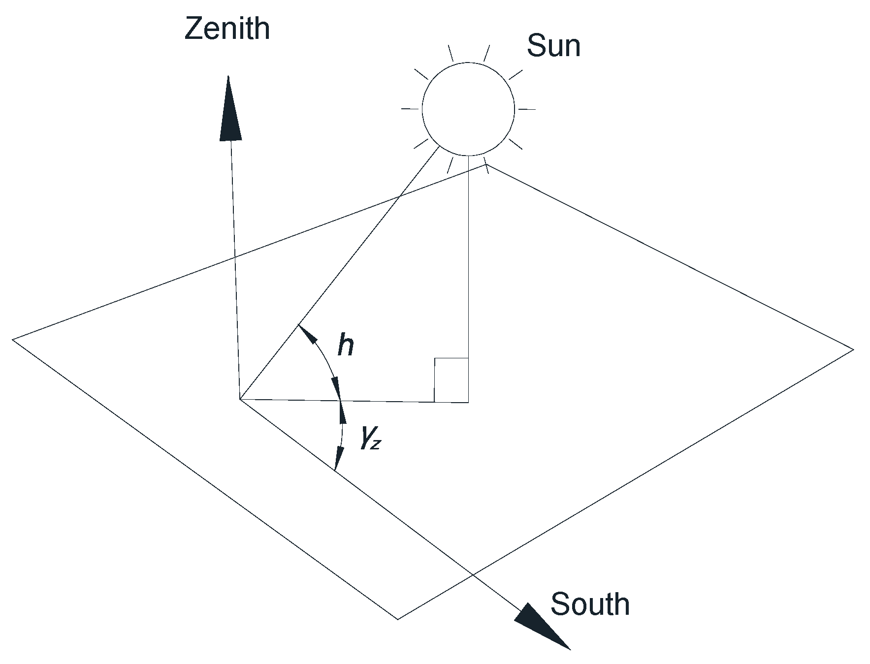
2.2.3. Solar Altitude Angle h

Solar altitude angle refers to the structure and the Sun’s center line and the horizontal plane of the line angle, the Sun’s incidence direction, and the angle of the horizontal plane. The solar altitude angle h changes with time, and the relationship between the angles can be seen in Figure 1, which is calculated as follows:
sin h = cos φ cos δ cos ω + sin φ sin δ
where φ is the geographic latitude, normalized to north latitude; δ is the solar declination angle; and ω is the solar time angle.

2.2.4. Solar Azimuth γz

Solar azimuth refers to the angle between the projection of incident light on the ground and the due south direction, and it is specified that the solar azimuth γz is positive when it deviates from the east, and its specific calculation equation is as follows:
sin γ z = cos δ sin ω cos h
where δ is the solar declination angle; ω is the solar time angle; and h is the solar altitude angle.

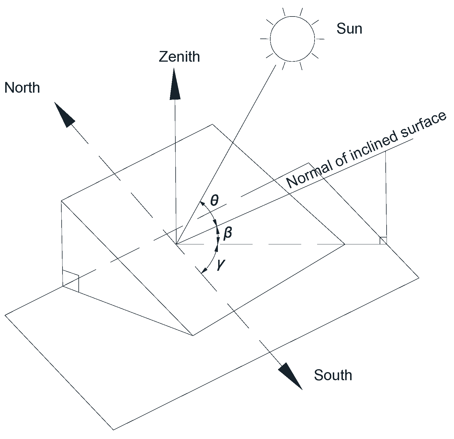
2.2.5. Solar Incidence Angle θ

The solar incidence angle θ is the angle between the incident light and the plane normal. The solar incidence angle of any plane with the structure of the plane normal to the tilt angle β and azimuth γ. The geometric relationship between the three shown in Figure 2. The solar incidence angle can be calculated using the following equation:
cos θ = sin β sin h + cos β cos h cos γ z γ
where β is the angle between any plane normal and the horizontal plane; h is the solar altitude angle; γz is the solar azimuth angle; and γ is the azimuth of any out-of-plane normal.

2.3. Boundary of Solar Radiation Intensity

2.3.1. Direct Solar Radiation

Based on the above theoretical basis, the direct solar radiation reaching the Earth’s surface can be expressed in the following equation:
I s = I 0 P 1 / sin h
where P is the atmospheric transparency coefficient and h is the solar altitude angle.
Assuming that the north, west, and up directions of the Sun correspond to the x, y, and z directions in the Cartesian coordinate system, the direction vector of the Sun in three-dimensional coordinates can be obtained based on the Sun angle calculated above, and the conversion relationship between the Sun angle and the direction vector is:
i x = cos 90 ° h sin γ z
i y = sin 90 ° h sin γ z
i z = cos γ z
Because of the shading effect, the direct solar radiation does not cover the entire structure. The shading effect is illustrated in Figure 3. Shading increases the structural temperature gradient and internal stresses, leading to more complex numerical analyses [16]. The solar irradiated and shaded areas are divided by the solar radiation direction vector.
The direct solar radiation in the shaded region is 0 and the direct solar radiation received in the sunlit region is ID:
I D = I s cos β

2.3.2. Atmospheric Scattering Radiation

A portion of the solar radiant energy is absorbed by the atmosphere during its transfer to the Earth’s surface, and a portion of this absorbed energy returns to the surface, it has been found that this portion of the energy is closely related with the surface inclination angle [17], and is not strongly related with the azimuthal angle of the structure surface, and the intensity of the scattering on the horizontal plane has been obtained as:
I d H = 0.271 I 0 0.294 I D sin h
The intensity of the Sun-scattered radiation in a cross-section with an arbitrary inclination angle β is:
I d = 1 + cos β 2 I d H

2.3.3. Surface-Reflected Radiation

A portion of the energy radiated by the Sun at the surface will be reflected by the surface and then projected the surface of the bridge structure. The equation used is the following:
I f = ξ I D sin h + I d H 1 cos β 2
where ξ is the ground reflection coefficient, generally taken as 0.2.
In summary, the solar shortwave radiation projected onto the surface of a structure can be categorized as direct solar radiation, atmospheric scattering, and surface reflection, and the total solar radiant energy qs on any surface is given in the following equation:
q s = a t I D + I d + I f
where at is the short-wave radiation absorptivity of concrete.

3. Boundary of Convective Heat Transfer

The convective heat transfer between the surface of the concrete box girder and the outside atmosphere follows Newton’s law of cooling, as follows:
q c = h c T a T
where hc is the convective heat transfer coefficient.
The convective heat transfer coefficient is calculated according to the convective heat transfer coefficient correlation equation in the literature [18]. In the case of no wind or very small wind speed, the outer surface of the box girder and the atmosphere are mainly characterized by natural convection heat transfer. The convective heat transfer coefficient can be calculated using the following equation:
h = k L 0.68 + 0.67 ( cos φ R a L ) 1 / 4 1 + 0.492 k μ C p 9 / 16 4 / 9 i f   R a L 10 9 k L 0.825 + 0.387 R a L 1 / 6 1 + 0.492 k μ C p 9 / 16 8 / 27 2 i f   R a L > 10 9
where L is the characteristic length (the horizontal plane is the ratio of area to perimeter, the inclined plane is the height), k is the coefficient of thermal conductivity, φ is the angle between the calculation surface and the vertical plane, μ is the dynamic viscosity, Cp is the specific heat capacity, RaL is the Rayleigh number, which can be calculated by the following equation:
R a L = g α p ρ 2 C p T T e x t L 3 k μ
where g is the gravitational acceleration, αp is the coefficient of thermal expansion, ρ is the density, T is the structural temperature, and Text is the atmospheric temperature.
When the wind speed is large, and there is forced convection heat transfer between the outer surface of the box beam and the atmosphere, the convection heat transfer coefficient can be calculated using the following equation:
h = 2 k L 0.3387 P r 1 / 3 R e L 1 / 2 1 + 0.0468 P r 2 / 3 1 / 4 i f   R e L 5 × 10 5 2 k L P r 1 / 3 0.037 R e L 4 / 5 871 i f   R e L > 5 × 10 5
where L is the length of the calculation surface; Pr is the Prandtl number, calculated by the formula Pr = μCp/k; ReL is the Reynolds number, calculated by the formula ReL = ρUL/μ, where U is the external fluid flow rate, which is the wind speed in the natural environment.
The inside of the box girder is a closed space, and the inner surface of the box girder mainly carries out internal natural convection heat transfer with the gas inside the box, which can be calculated by the following equation:
h = k H 1 24 R a L
where H is the height of the internal region and L is the width of the internal region.

4. Boundary of Radiative Heat Transfer

Radiant heat transfer of box girders in the natural environment mainly consists of absorption and reflection, and the absorbed radiant heat includes atmospheric scattering and ground diffuse reflection.

4.1. Environmental Radiation

The atmospheric radiant heat Ga received by the bridge structure is calculated by the following equation:
G a = ε a σ T e x t 4
where Ɛa is the atmospheric radiation coefficient, which is usually taken as 0.82, and σ is the blackbody radiation constant, which has a value of 5.67 × 10⁻⁸ W/(m2·K4).
The heat radiated from the surface by the surface with an inclination angle of β is calculated by the following equation:
U β = σ T e x t 4 1 cos β 2

4.2. Structural Exothermic Radiation

Structure absorbs external radiant heat simultaneously and also radiates heat to the outside. The radiant heat El can be calculated according to the following equation:
E l = a l σ T 4
where al is the long-wave radiation absorptivity and emissivity of concrete.
In summary, the total amount of radiative heat transfer qr of concrete can be expressed as:
q r = a l G a + U β E l

5. Engineering Background and Verification

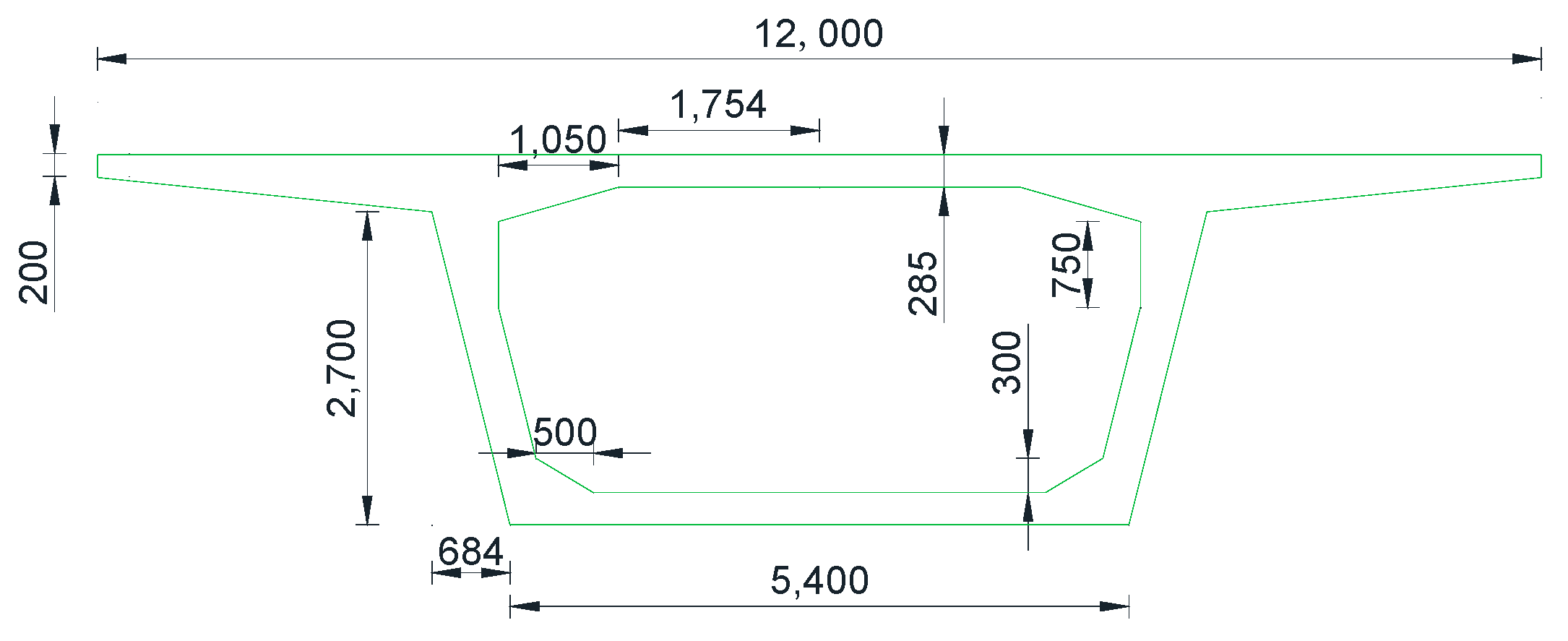
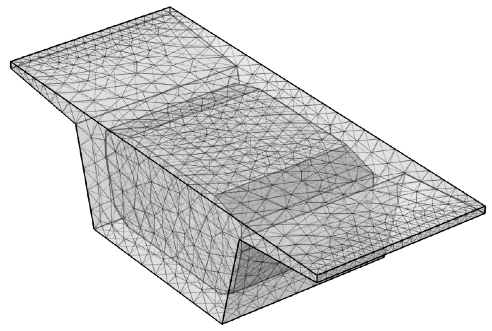
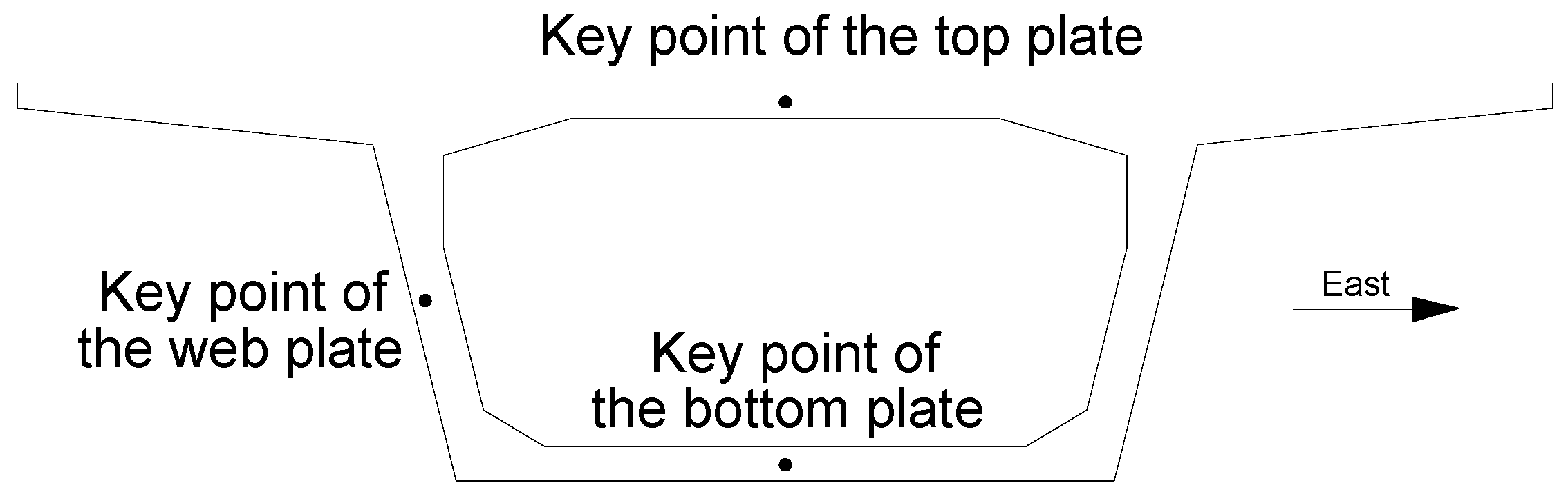
5.1. Engineering Background

A 32 m simply supported girder bridge of a passenger dedicated line in the literature [19] was taken as an example of calculation. The bridge was located at longitude 117.97° E, latitude 28.45° N, and the bridge azimuth was 6.92°. The cross-sectional dimensions of the box girder are shown in Figure 4. The girder was made of C50 concrete material, which has a thermal conductivity of 10.8 kj/(h·K·m). The thermal conductivity of air was 0.0864 kj/(h·K·m), the atmospheric transparency coefficient was 0.8, and the wind speed was 2.5 m/s. The short-wave absorptivity and emissivity of concrete was 0.6, and the long-wave absorptivity and albedo were 0.85. The reflectivity of the ground surface was 0.18.
The temperature change during the day is usually influenced by the Sun; the temperature reaches its maximum value during the day and its minimum value at night. In general, the variation in the temperature during the day can be described by a sinusoidal function with the function equation:
T e x t = T m a x + T m i n 2 + T m a x T m i n sin A t B
where Tmax is the daily maximum temperature; Tmin is the daily minimum temperature; A is the angular frequency, A = 2π/T; and B is the phase offset, which is used to adjust the starting point of the waveform, and the temperature is lowest at 3:00 a.m. in the calculation time.
The model calculated once every hour and the calculation results gradually stabilized after multiple iterations. One week of analysis met the requirements of temperature field simulation [20]. The calculation period was from 27 December 2013 to 2 January 2014, and the daily maximum and minimum temperatures and the atmospheric sine function are shown in Table 1. Figure 5 shows a plot of the atmospheric sine function for the seven days of the calculation period.
Combined with the boundary condition calculation method introduced above and the engineering background of the example, the outer surface of the box girder applied solar radiation, external natural convection, and radiative heat transfer boundaries. The internal cavity applied internal natural convection boundaries. The three-dimensional temperature field finite element model of the box girder was established using COMSOL V6.1 software, as shown in Figure 6.

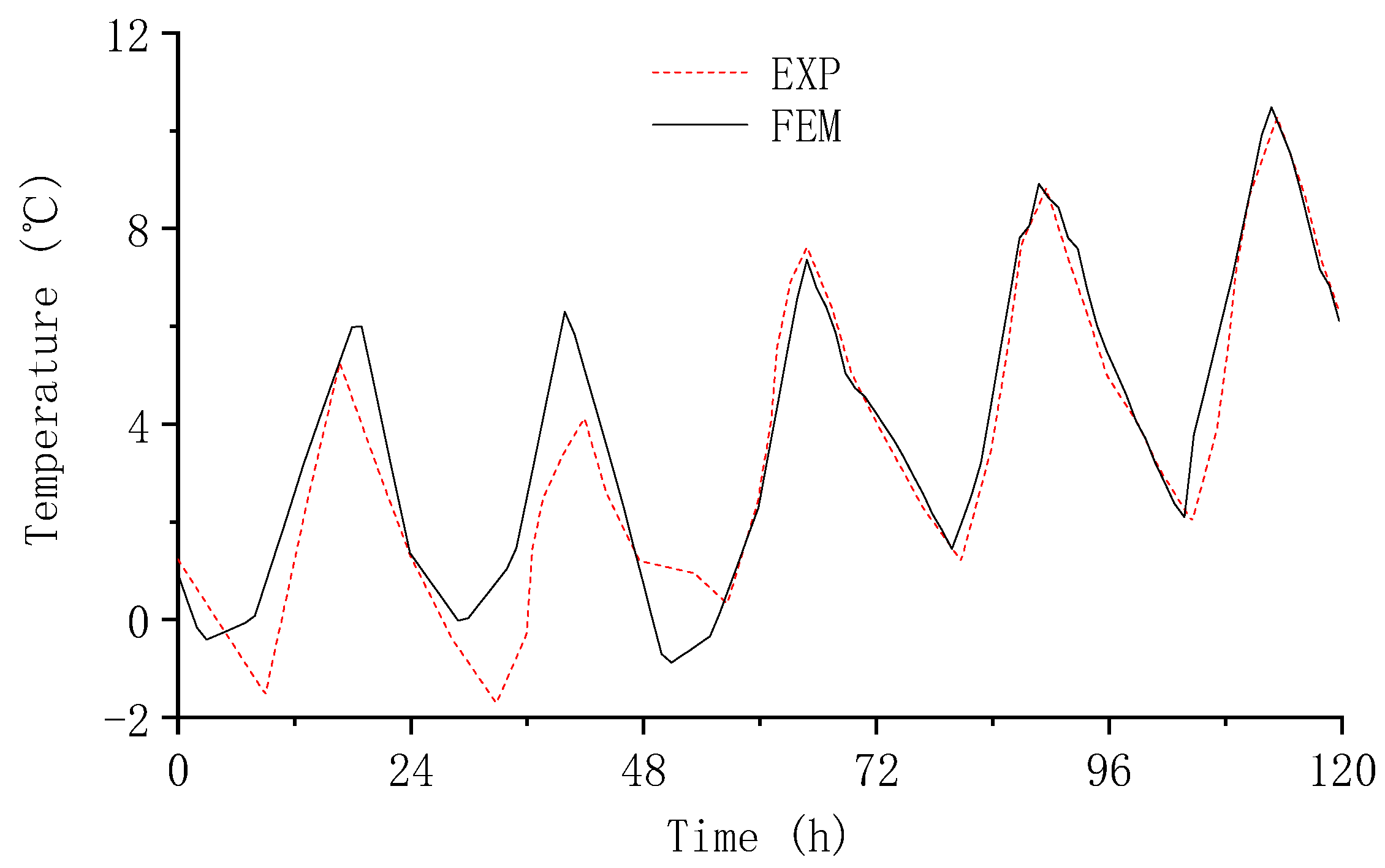
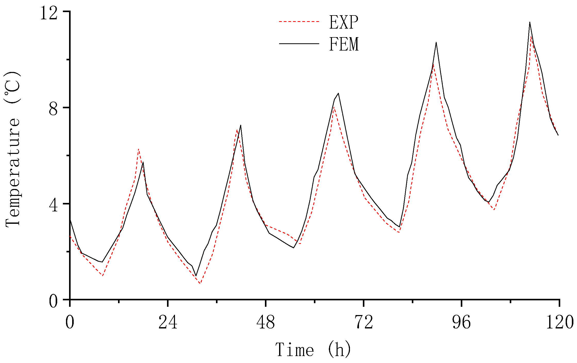
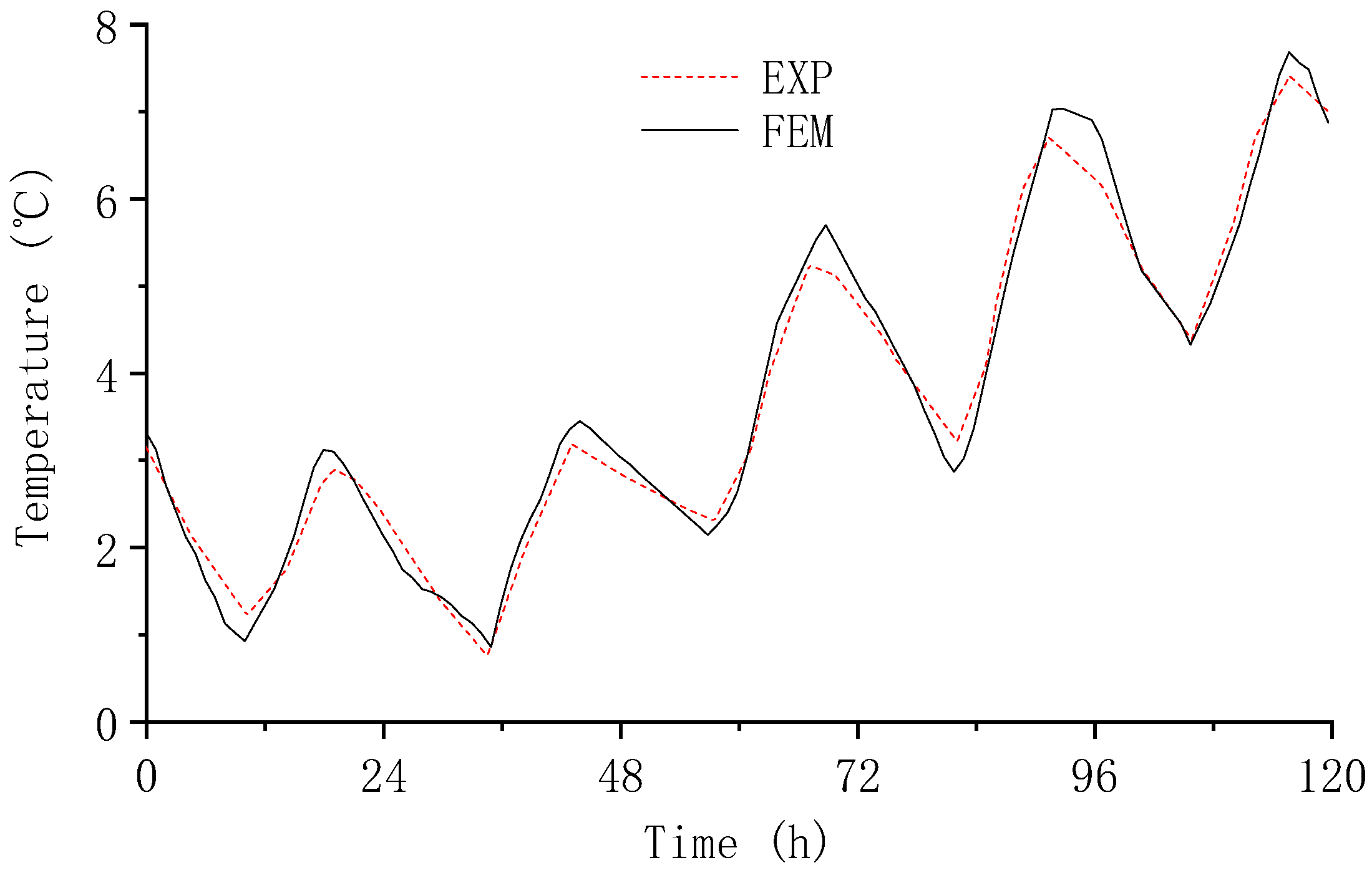
5.2. Validation of Results

The above boundary conditions and parameters were used to simulate the temperature field of the box girder. Data from the middle 5 days were selected for analysis; the first and last days were removed to reduce the influence of boundary effects. Comparison of the finite element results (FEM) and experimental data (EXP) of the key points of the box girder top plate, web plate, and bottom plate was conducted. The locations of key points are shown in Figure 7, and the results are compared in Figure 8, Figure 9 and Figure 10.
As can be seen from Figure 8, Figure 9 and Figure 10, the calculated and measured results of the temperature distribution at each key point of the box girder have a good coincidence. The temperature at the key point of the top plate had a slight difference in the first two days, and the maximum error between the calculated value and the measured value was 2.4 °C. In the last three days, the calculated value and the measured value matched well, and the maximum error was only 0.3 °C. The temperature at the key point of the web plate was 0.5 °C, and the maximum error between the calculated value and the measured value was 0.5 °C. The maximum error between the calculated and measured values of the key point temperature of the web plate was 0.5 °C. The maximum error between the calculated and measured temperatures of the key points of the bottom plate was 0.8 °C. Under comprehensive consideration, the error between the calculated and measured results was small; thus, the boundary condition calculation method used in this paper can effectively simulate the three-dimensional temperature field distribution of the box girder.

6. Influence of Boundary Condition Parameters on the Temperature Field Distribution

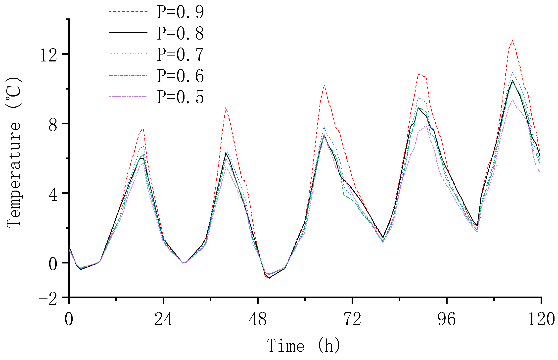
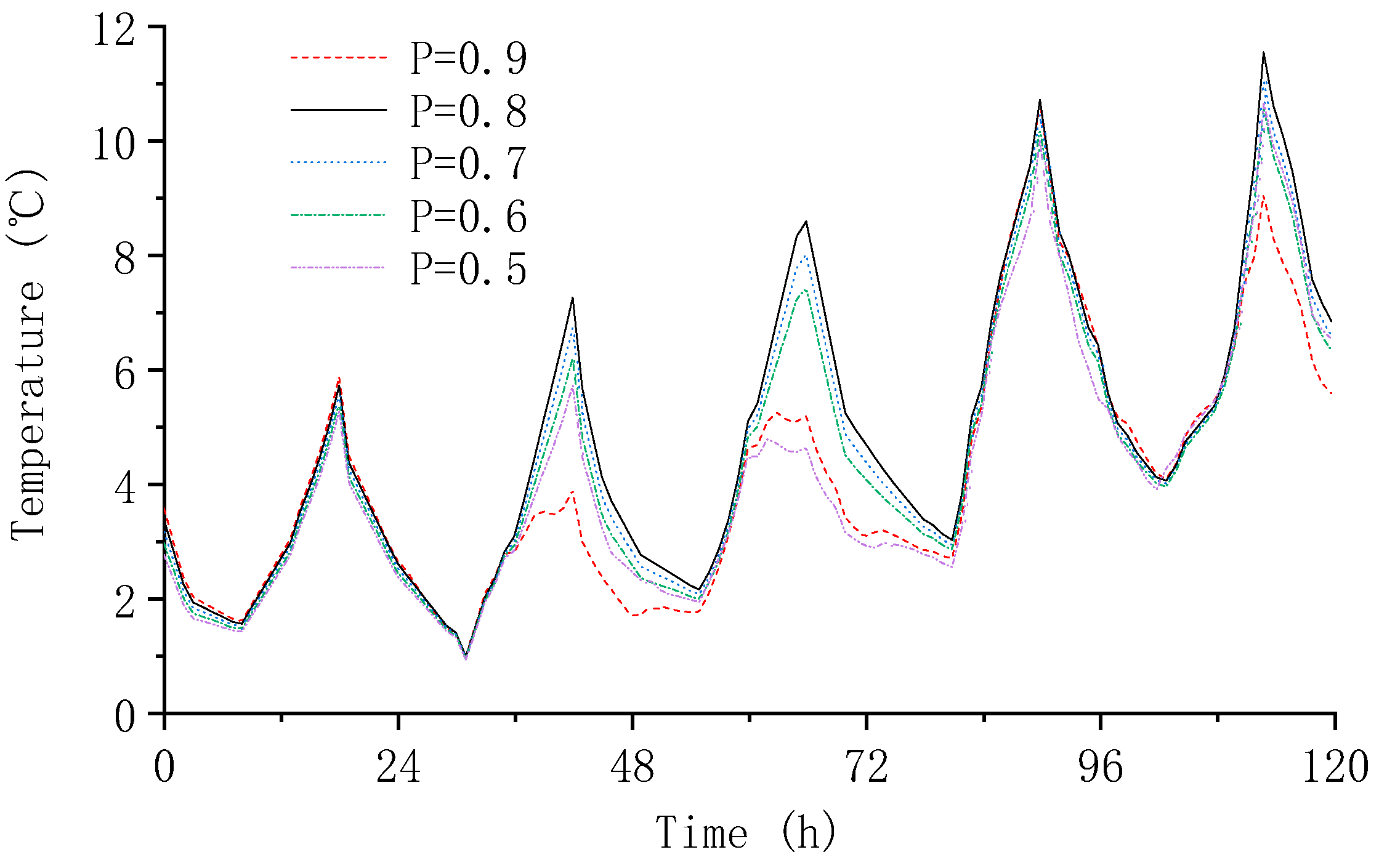
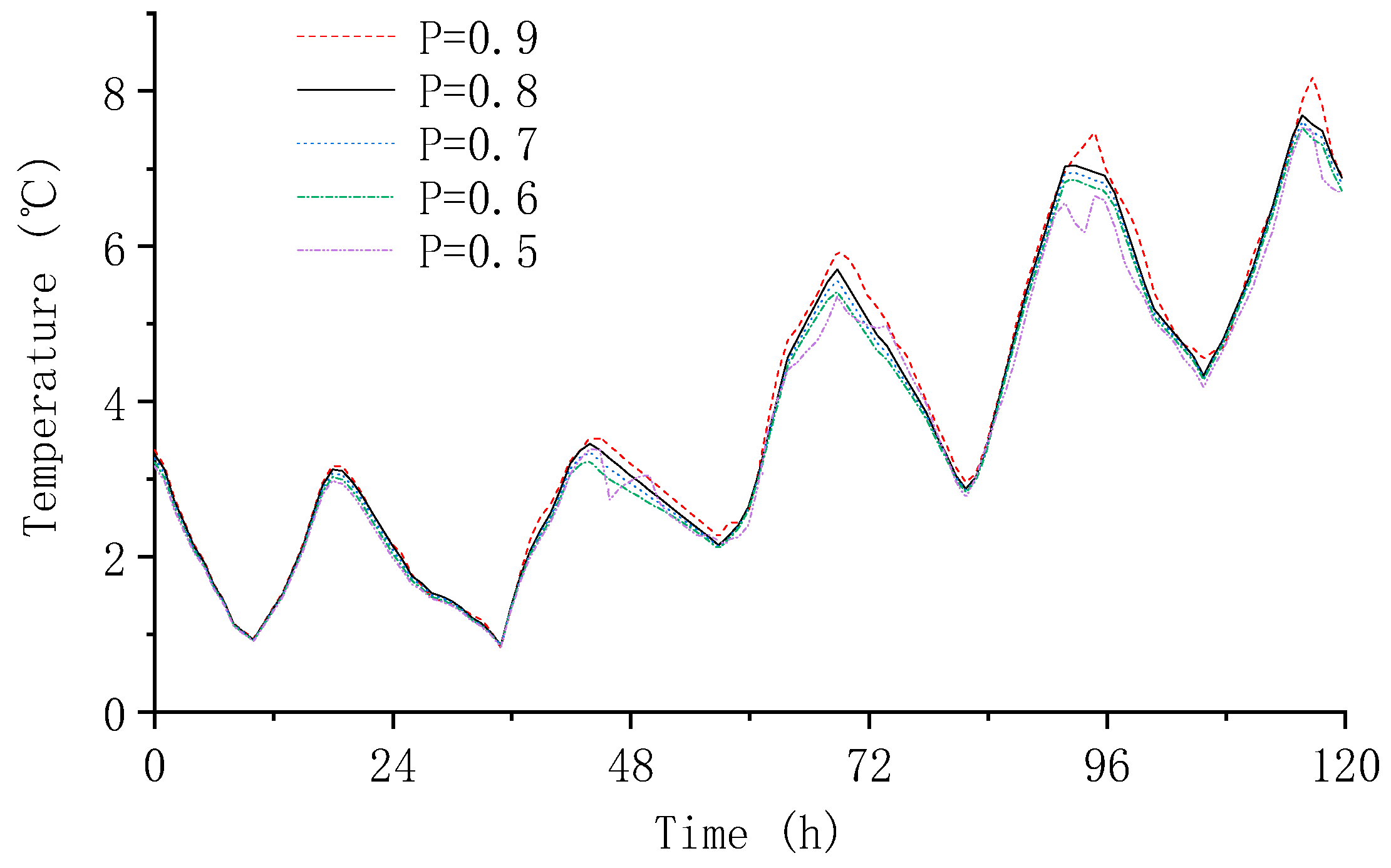
6.1. Impact of Atmospheric Transparency

The atmospheric transparency coefficient is a parameter that measures the ability of the atmosphere to transmit solar radiation, which affects the size of the bridge structure by the direct radiation and scattered radiation from the Sun. This paper analyzed the atmospheric transparency coefficient P by setting it to five values of 0.9, 0.8, 0.7, 0.6, and 0.5 to explore the effect of atmospheric transparency on the temperature field distribution of the box girder structure. Figure 11, Figure 12 and Figure 13 show the temperature maps of key points of the box girder at different atmospheric transparency coefficients.
As shown in Figure 11, because the atmospheric transparency directly affects the magnitude of solar radiation received by the box girder, the top plate irradiated by the Sun reflects a large correlation with the atmospheric transparency in the temperature distribution. The daily maximum temperature at the key point of the top plate is greatly affected by the change in atmospheric transparency, and it increases with the increase in the atmospheric transparency coefficient. When the atmospheric transparency coefficient increases from 0.8 to 0.9, the daily maximum temperature of the key point of the roof plate on the third day increases from 7.3 °C to 10.3 °C, with an increase of 41.1%. The daily minimum temperature and the change pattern of temperature were less affected.
The daily maximum temperature of the key point temperature of the web plate increases with the increase in the atmospheric transparency coefficient from 0.5 to 0.8. However, when the atmospheric transparency coefficient increases to 0.9, the daily maximum temperature decreases abruptly, which is presumed to be due to the fact that the web plate is subjected to both direct solar radiation and scattered radiation, and the effect of scattered radiation decreases significantly when the atmospheric transparency coefficient reaches 0.9, which leads to a decrease in the daily maximum temperature.
Because the bottom plate is always in the shaded area, the temperature distribution at the key point of the bottom plate is minimally affected by the atmospheric transparency. As can be seen from Figure 13, the temperature curves at the key points of the bottom plate at different atmospheric transparency coefficients basically overlap, and the daily maximum temperature at the key points of the bottom plate only changes slightly when P = 0.9 and P = 0.5, and the value of the key point temperature change ranges from −0.8 °C to 0.6 °C. The temperature distribution at the key points of the bottom plate is also affected by the atmospheric transparency coefficient.
In summary, atmospheric transparency has the greatest effect on the top plate temperature, and the maximum daily temperature of the top plate increases with the increase in the atmospheric transparency coefficient. Atmospheric transparency also has less influence on the temperature of the web plate and has the least influence on the temperature of the bottom plate. When the atmospheric transparency coefficient is too large or too small, the maximum daily temperature of the web plate will appear to decrease abruptly.

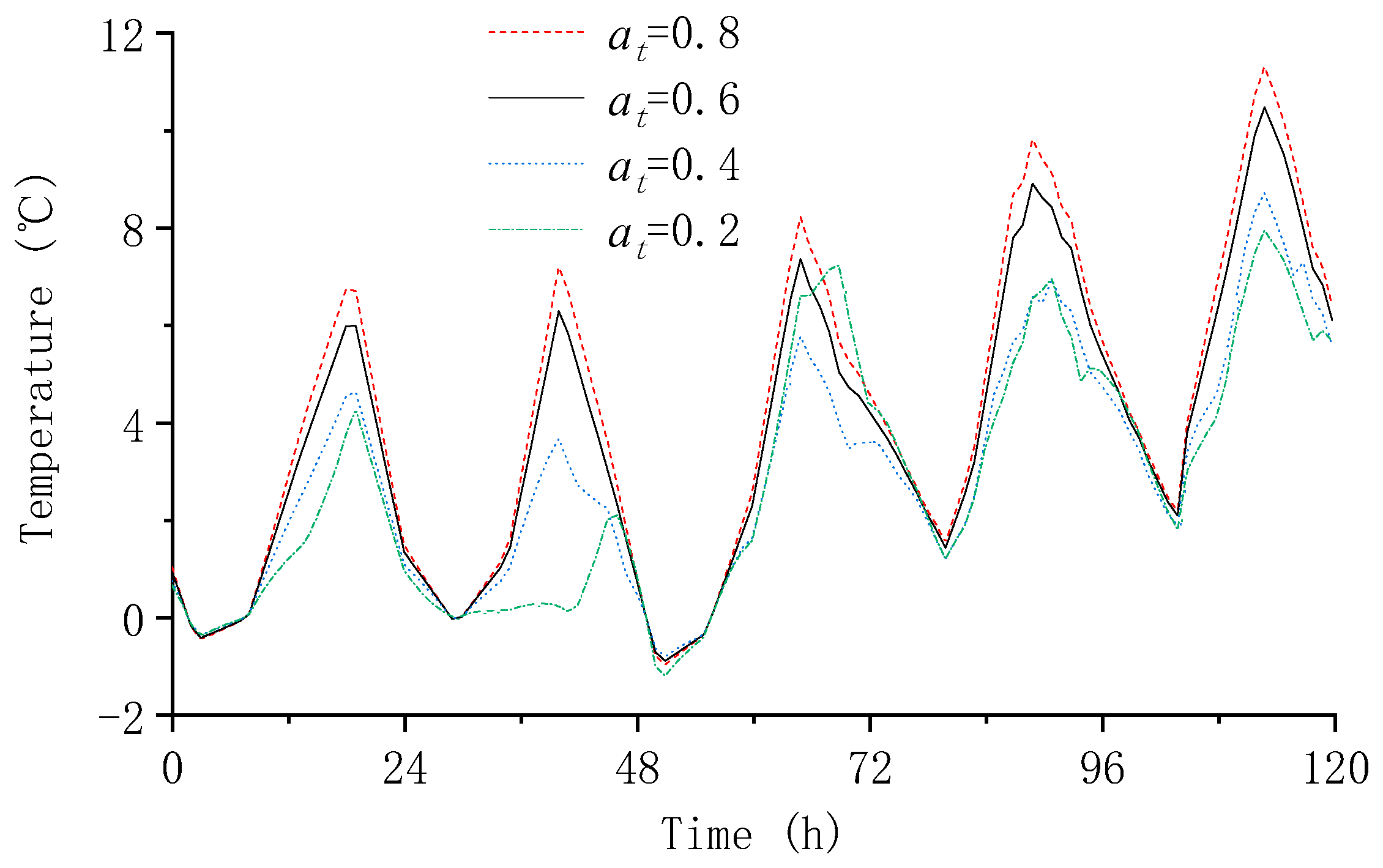
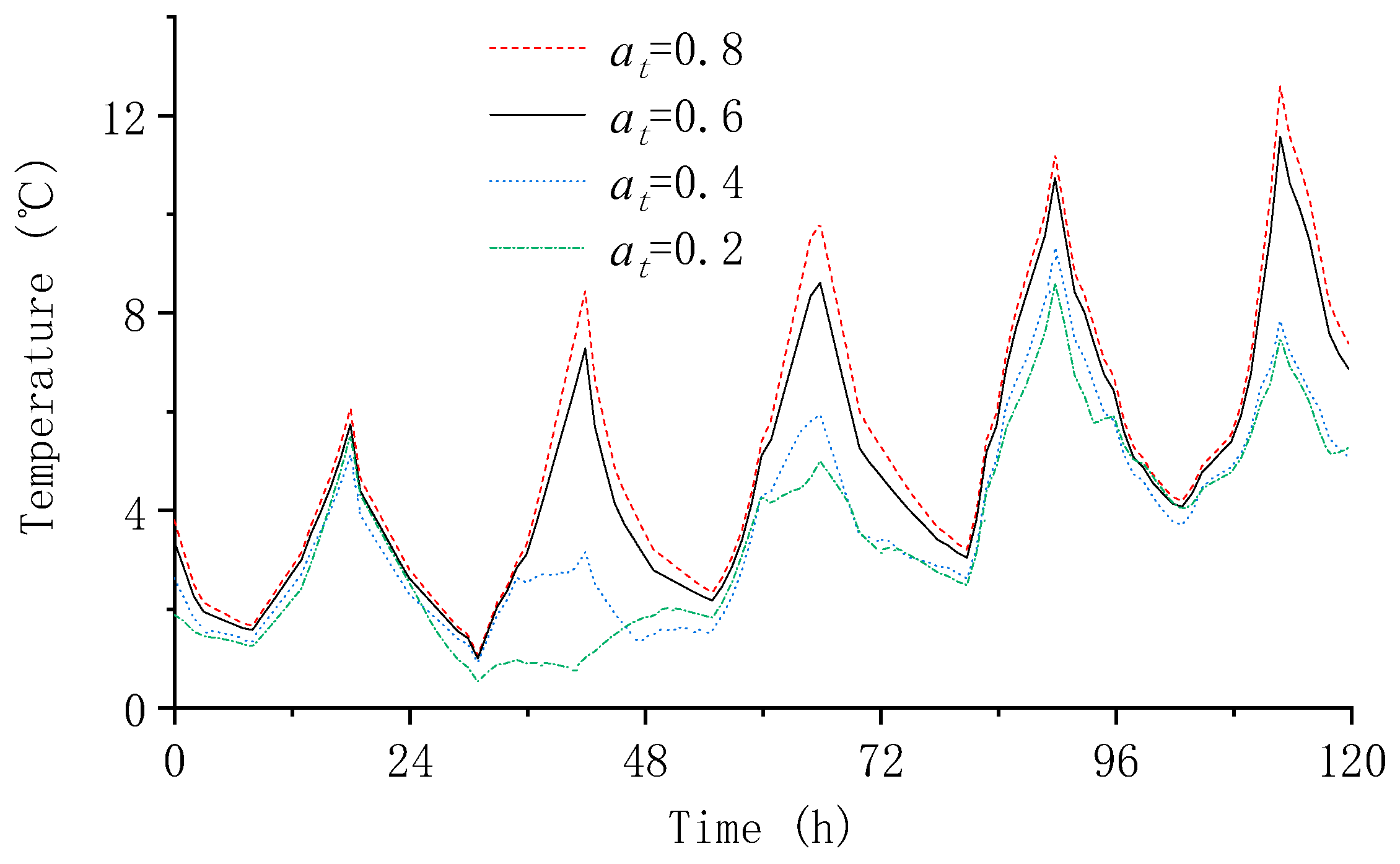
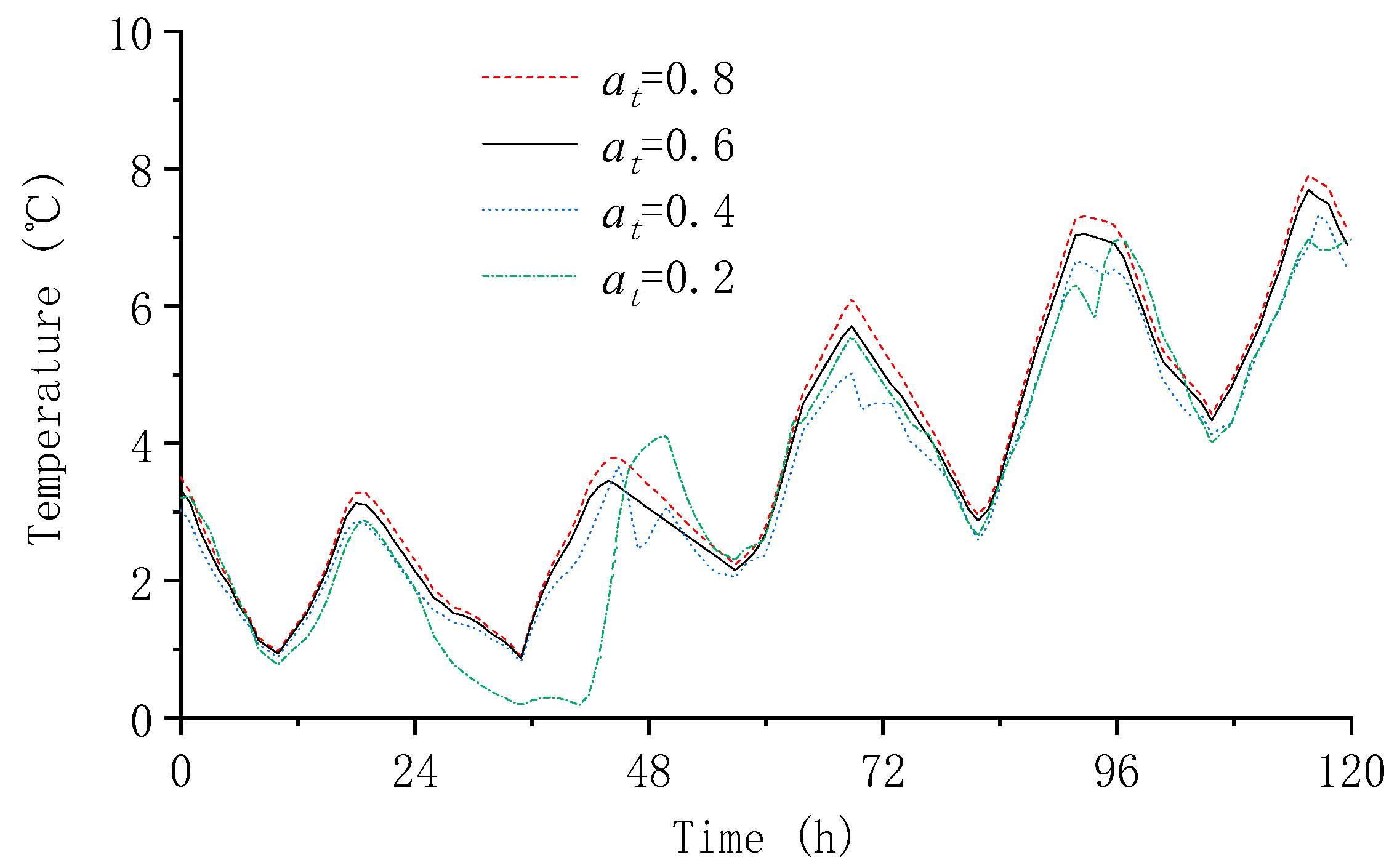
6.2. Influence of Short-Wave Absorptivity in Concrete

Short-wave absorptance of concrete refers to the proportion of short-wave radiation (mainly solar radiation) absorbed by concrete material. In this study, the influence of the short-wave absorptance of concrete on the temperature field distribution of a box girder structure was explored by setting the short-wave absorptance of concrete to four values of 0.8, 0.6, 0.4, and 0.2. Figure 14, Figure 15 and Figure 16 show the temperature diagrams of key points of the box girder at different short-wave absorptivity.
As can be seen in Figure 14 and Figure 15, the short-wave absorptivity of concrete has a more significant effect on the temperatures of the top and web plate. When the short-wave absorptivity decreased from 0.6 to 0.4, the temperatures of the top and web plate decreased significantly. The maximum decrease in the temperature of the top plate reached 41.8%, and the maximum decrease in the temperature of the web plate reached 57.1%.
As can be seen in Figure 16, the bottom plate temperature is less affected by the short-wave absorptivity. Although there is a small decrease in the bottom plate temperature as the short-wave absorptivity decreases, the regularity is not obvious.
In summary, the short-wave absorptivity of concrete can significantly affect the temperature distribution of concrete box girders, and the temperatures of the top plate and web plate decrease with the decrease in the short-wave absorptivity of concrete. When designing box girders, the structural temperature can be reduced covering the structural surface with materials with low short-wave absorptivity.

7. Discussion

In order to explore the boundary conditions for the three-dimensional temperature field of box girders in natural environments, a series of studies were carried out in this paper.
Firstly, based on the theoretical basis of engineering thermodynamics, three kinds of temperature field boundary conditions of solar radiation, convective heat transfer, and radiative heat transfer of box girder under natural environment were investigated, respectively, which comprehensively considered the factors of direct solar radiation, atmospheric scattering, ambient radiation, structural shading effect, and convective heat transfer.
Secondly, taking a box girder of a section of railroad line as an example, the boundary condition calculation method in this study was used to establish a finite element model. The structural temperature field distribution was analyzed and verified with measured temperature data. The calculation results are in good agreement with the measured results, and the model can effectively simulate the three-dimensional temperature field distribution of the box girder.
Finally, the effects of the atmospheric transparency coefficient and concrete short-wave absorptivity on the temperature field distribution of box girders are discussed. The atmospheric transparency has the greatest effect on the temperature of the top slab and the least effect on the temperature of the bottom slab. The daily temperature maximum of the top plate increases with the increase in the atmospheric transparency coefficient. Atmospheric transparency also has a certain influence on the temperature of the web plate. When the atmospheric transparency coefficient is too large or too small, the daily maximum temperature of the web plate will appear to decrease abruptly. The short-wave absorptivity of concrete can significantly affect the temperature distribution of the concrete box girder, and the temperature of the top plate and web plate decreases with the decrease in the short-wave absorptivity of concrete. When designing box girders, the structural temperature can be reduced covering the structural surface with materials that have low short-wave absorptivity.

Author Contributions

Conceptualization, B.Y.; methodology, B.Y.; software, H.F.; validation, B.Y., H.F. and H.S.; formal analysis, H.F.; writing—original draft preparation, B.Y., H.F. and H.S.; writing—review and editing, H.F., H.S. and B.H. All authors have read and agreed to the published version of the manuscript.

Funding

This research was funded by the National Natural Science Foundation of China (grant number 52278470) and the Natural Science Foundation of Hunan Province (grant number 2022JJ30741).

Institutional Review Board Statement

Not applicable.

Informed Consent Statement

All authors are aware of and agree with the publication of the paper.

Data Availability Statement

The original contributions presented in this study are included in the article. Further inquiries can be directed to the corresponding author.

Acknowledgments

The authors would like to thank the National Natural Science Foundation of China (Project No. 52278470) and the Natural Science Foundation of Hunan Province (Project No. 2022JJ30741).

Conflicts of Interest

The authors declare no conflicts of interest.

References

  1. Peeters, B.; De, R. One-year monitoring of effects versus damage the Z24-Bridge: Environmental events. Earthq. Eng. Struct. Dyn. 2001, 30, 149–171. [Google Scholar] [CrossRef]
  2. Ni, Y.; Hua, X.; Fan, K.; Ko, J.M. Correlating modal properties with temperature using long-term monitoring data and support vector machine technique. Eng. Struct. 2005, 27, 1762–1773. [Google Scholar] [CrossRef]
  3. Dai, G.; Wang, F.; Ge, H.; Xiao, Y.; Rao, H. Temperature pattern and extreme value of concrete high pier of high-speed railway bridge. Tiedao Kexue Yu Gongcheng Xuebao 2023, 20, 961–972. [Google Scholar]
  4. Huang, S.; Cai, C.; Zou, Y.; He, X.; Zhou, T.; Zhu, X. Experimental and Numerical Investigation on the Temperature Distribution of Composite Box-girders with Corrugated Steel Webs. Struct. Control. Health Monit. 2022, 29, e3123. [Google Scholar] [CrossRef]
  5. Zhang, F.; Liu, J.; Gao, L. Experimental Investigation of Temperature Gradients in a Three-Cell Concrete Box-Girder. Constr. Build. Mater. 2022, 335, 127413. [Google Scholar]
  6. Zhang, P.; Wang, C.; Wu, G.; Wang, Y. Temperature Gradient Models of Steel-Concrete Composite Girder Based on Long-Term Monitoring Data. J. Constr. Steel Res. 2022, 194, 107309. [Google Scholar] [CrossRef]
  7. Fan, J.; Li, B.; Liu, C.; Liu, Y.-F. An Efficient Model for Simulation of Temperature Field of Steel-Concrete Composite Beam Bridges. Structures 2022, 43, 1868–1880. [Google Scholar] [CrossRef]
  8. Elshoura, A.; Okeil, A. Calibration of Temperature Gradient Load Factor for Service Limit State Design of Concrete Slab-on-Girder Bridges. J. Bridge Eng. 2022, 27, 04022112. [Google Scholar] [CrossRef]
  9. Liu, Y.; Ma, Z.; Liu, J.; Zhu, W.; Wang, X.; Li, M. Temperature action and zoning of concrete jointless bridge in Shanxi. J. Traffic Transp. Eng. 2022, 22, 85–103. [Google Scholar]
  10. Zhu, Y.; Sun, D.; Shuang, M. Investigation of temperature-induced effect on rail-road suspension bridges during operation. J. Constr. Steel Res. 2024, 215, 108542. [Google Scholar] [CrossRef]
  11. Dai, G.; Wang, F.; Chen, Y.; Ge, H.; Rao, H. Modelling of extreme uniform temperature for high-speed railway bridge piers using maximum entropy and field monitoring. Adv. Struct. Eng. 2023, 26, 302–315. [Google Scholar] [CrossRef]
  12. Zhang, L.; Zhou, L.; Bu, J.; Liu, Q.; Wei, B.; Zhao, C.B.; Chai, W. Temperature gradient estimation of long-span concrete box girders using average conditional exceedance rate function. Struct. Infrastruct. Eng. 2024, 1–15. [Google Scholar] [CrossRef]
  13. Yang, D.; Guan, Z.; Yi, T.; Li, H.-N.; Liu, H. Structural temperature gradient evaluation based on bridge monitoring data extended by historical meteorological data. Struct. Health Monit. 2024, 23, 1800–1815. [Google Scholar] [CrossRef]
  14. Zhang, H.; Liu, D.; Zhao, W.; Ding, S.; Liu, Y.; Yang, J.; Lu, W. Boundary Condition and Distribution Study of Temperature Field of Rail-Cum-Road Steel Truss Girder. Zhongguo Tiedao Kexue 2023, 44, 91–101. [Google Scholar]
  15. Zhao, R.; Wang, Y. Studies on Temperature Field Boundary Conditions for Conerete Box girder Bridges Under Solar Radiation. Zhongguo Gonglu Xuebao 2016, 29, 52–61. [Google Scholar]
  16. Zhu, J.; Chen, K.; Meng, Q. Fine Analysis Method for Spatial Temperature Field of Long-Span Suspension Bridge. Tianjin Daxue Xuebao 2018, 51, 339–347. [Google Scholar]
  17. Peng, Y. Studies on Theory of Solar Radiation Thermal Effects on Concrete Bridges with Application. Ph.D. Dissertation, Southwest Jiaotong University, Chengdu, China, 2007. [Google Scholar]
  18. Incropera, F.; DeWitt, D.; Bergman, T.; Lavine, A.S. Fundamentals of Heat and Mass Transfer, 6th ed.; John Wiley & Sons: Hoboken, NJ, USA, 2006. [Google Scholar]
  19. Liu, Y.; Su, H.; Dai, G. Study on Temperature Fields of Simply-supported Box Girder under Solar Radiation in Passenger Dedicated Lines Based on Meteorological Conditions. Tiedao Xuebao 2019, 14, 154–159. [Google Scholar]
  20. Dai, G.; Zheng, P.; Yan, B.; Xiao, X.N. Longitudinal Force of CWR on Box Girder under Solar Radiation. Zhejiang Daxue Xuebao 2013, 47, 609–614. [Google Scholar]
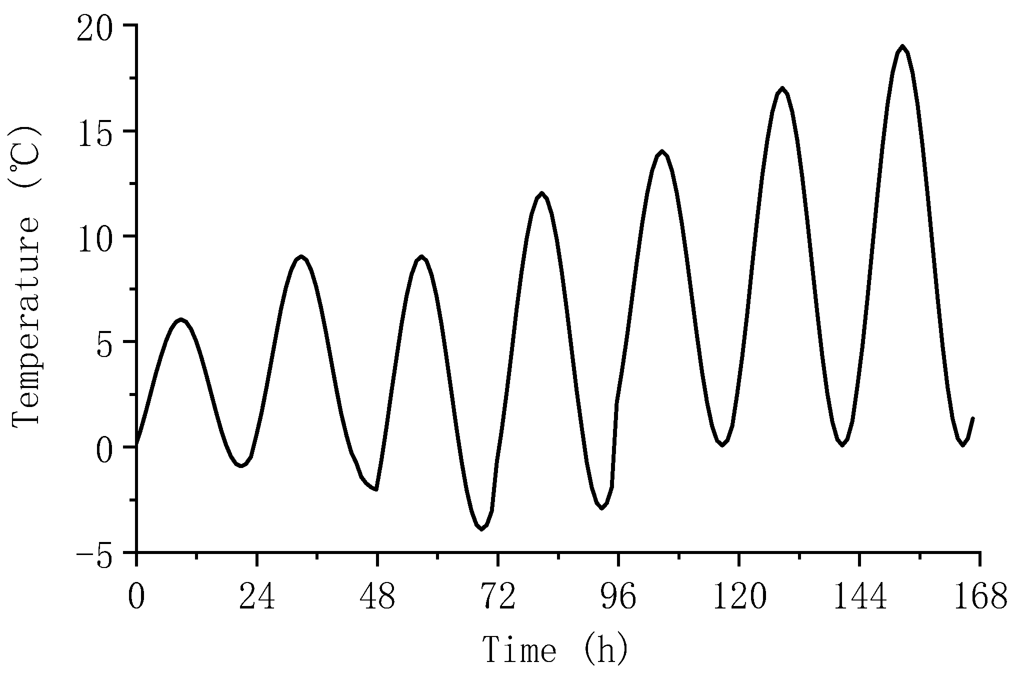
Figure 1. Solar altitude angle and azimuth angle.
Applsci 15 01378 g001
Figure 2. Angle of incidence of the Sun in an arbitrary plane.
Applsci 15 01378 g002
Figure 3. Solar radiation shading effect.
Applsci 15 01378 g003
Figure 4. Cross-section of the box girder (unit: mm).
Applsci 15 01378 g004
Figure 5. Atmospheric sine function.
Applsci 15 01378 g005
Figure 6. Three-dimensional temperature field finite element model of the box girder.
Applsci 15 01378 g006
Figure 7. Map of key point locations.
Applsci 15 01378 g007
Figure 8. Critical point temperatures of the top plate.
Applsci 15 01378 g008
Figure 9. T Critical point temperatures of the web plate.
Applsci 15 01378 g009
Figure 10. Critical point temperatures of the bottom plate.
Applsci 15 01378 g010
Figure 11. Critical point temperatures of the top plate for different atmospheric transparency coefficients.
Applsci 15 01378 g011
Figure 12. Critical point temperatures of the web plate for different atmospheric transparency coefficients.
Applsci 15 01378 g012
Figure 13. Critical point temperatures of the bottom plate for different atmospheric transparency coefficients.
Applsci 15 01378 g013
Figure 14. Critical point temperatures of the top plate for different short-wave absorptivity.
Applsci 15 01378 g014
Figure 15. Critical point temperatures of the web plate for different short-wave absorptivity.
Applsci 15 01378 g015
Figure 16. Critical point temperatures of the bottom plate for different short-wave absorptivity.
Applsci 15 01378 g016
Table 1. Air temperatures during the calculation time.
Day/MonthMaximum TemperatureMinimum TemperatureAtmospheric Sine Function
27/126−1 T e x t 1 = 3.5 sin π t 12 π 4 + 2.5
28/129−1 T e x t 2 = 5 sin π t 12 π 4 + 4
29/129−4 T e x t 3 = 6.5 sin π t 12 π 4 + 2.5
30/1212−3 T e x t 4 = 7.5 sin π t 12 π 4 + 4.5
31/12140 T e x t 5 = 7 sin π t 12 π 4 + 7
1/1170 T e x t 6 = 8.5 sin π t 12 π 4 + 8.5
2/1190 T e x t 7 = 9.5 sin π t 12 π 4 + 9.5
Disclaimer/Publisher’s Note: The statements, opinions and data contained in all publications are solely those of the individual author(s) and contributor(s) and not of MDPI and/or the editor(s). MDPI and/or the editor(s) disclaim responsibility for any injury to people or property resulting from any ideas, methods, instructions or products referred to in the content.

