Abstract
Reliable analysis of remote photoplethysmography (rPPG) signals depends on identifying physiologically plausible pulses. Traditional approaches rely on clustering self-similar pulses, which can discard valid variability. Automating pulse quality assessment could capture the true underlying morphology while preserving physiological variability. In this manuscript, individual rPPG pulses were manually labelled as plausible, borderline and implausible and used to train multilayer perceptron classifiers. Two independent datasets were used to ensure strict separation between training and test data: the Vision-MD dataset (4036 facial videos from 1270 participants) and a clinical laboratory dataset (235 videos from 58 participants). Vision-MD data were used for model development with an 80/20 training–validation split and 5-fold cross-validation, while the clinical dataset served exclusively as an independent test set. A three-class model was evaluated achieving -scores of 0.92, 0.24 and 0.79 respectively. Recall was highest for plausible and implausible pulses but lower for borderline pulses. To test separability, three pairwise binary classifiers were trained, with ROC-AUC > 0.89 for all three category pairs. When combining borderline and implausible pulses into a single class, the binary classifier achieved an -score of 0.93 for the plausible category. Finally, usability analysis showed that automated labelling identified more usable pulses per signal than the previously used agglomerative clustering method, while preserving physiological variability.
1. Introduction
Photoplethysmography (PPG) is a non-invasive optical technique, widely used to estimate key vital signs, including heart rate (HR) and blood oxygen saturation (SpO2). PPG signals measure the reflected light from living tissue, which relates to the blood volume present within the optical path [1]. These signals can be recorded using specifically designed medical devices, such as pulse oximeters, but also using smart wearables. PPG signals are commonly extracted from the ear, wrist or finger. In recent years, remote PPG (rPPG) has emerged as a promising extension of this technology, allowing the extraction of PPG signals without direct contact with the skin [2]. This contactless approach holds significant potential for widespread, convenient health monitoring using everyday devices, such as smartphones or webcams, in a wide range of non-clinical environments [3]. In addition to measuring HR and SpO2, (r)PPG has been extensively researched to predict other vital signs non-invasively, such as blood pressure (BP) [4,5,6], blood glucose [4,7] and even intracranial pressure [8,9].
While rPPG has significant implementation advantages over PPG, it is not without its challenges. The remote nature of data capture makes rPPG highly susceptible to motion artifacts, lighting variations, sensor noise, and other environmental noises [10,11]. Understanding and working around noise in rPPG signals is critical for accurate vital sign estimation, especially for vital signs where waveform morphology is important (such as BP) [12].
To address the challenge of finding usable signals within noisy data, prior work has focused on the development of signal quality indicators (SQIs) that can be used to decide when a (r)PPG signal is usable for vital sign prediction. Approaches include amplitude or signal-to-noise ratio (SNR) based thresholds to evaluate the strength of the pulsatile component [13] across the full signal, as well as beat-by-beat or segmented approaches. For example, cross-correlation of consecutive pulse segments has been used to estimate signal quality by Karlen et al., aiming to identify self-similarity as a measure of signal quality [14]. Another method, proposed by Orphanidou et al., is aimed at accurate HR calculations and used within ECG and PPG, considers the time intervals of the individual beats to determine whether a reliable HR can be detected or not [15]. While this method is successful for HR detection, it does not consider the pulse morphology, which means further SQIs are required for, for example, BP prediction. Elgendi et al. used beat-to-beat morphology checks and found that, in particular, the skewness of a pulse was an indicator to whether a pulse was excellent, acceptable, or unfit [16].
Many of these SQIs operate at the full signal level (not per individual pulse), rely on additional extracted features, or depend on calibrated thresholds that are tuned to a specific dataset. These calibrated thresholds are typically tuned to the statistics of a particular dataset, but when acquisition conditions change (e.g., camera, sensor, or lighting conditions), the feature distributions also shift and the fixed threshold may no longer yield the intended results. Additionally, SQIs that rely on self-similarity may remove genuine morphological variability. In this work, we aim to automate the assessment of individual pulses across a varied dataset without the need for additional feature extraction.
To automate the assessment of individual pulse quality, human observers labelled each pulse as plausible, borderline, or implausible. These labels are used to train classifiers as a proof-of-concept to demonstrate that pulse quality assessment can be automated without the need for additional feature extraction, distinguishing between clean, physiologically meaningful pulses and those either degraded by noise or not containing any physiological information at all. We aim to demonstrate that the three categories are individually separable but also train a classifier aimed at the deployment within a vital sign prediction pipeline that separates plausible pulses from non-usable pulses (the borderline and implausible categories combined).
The content of this manuscript is organised as follows: Section 2 describes the methodology, including the data acquisition, pre-processing steps, pulse scoring process, and the evaluation metrics used in this study. Section 3 presents the results for the different classification tasks, providing an analysis of the classifiers’ performance in automatically labelling individual rPPG pulses’ quality. Section 4 details a discussion of these findings, highlighting the strengths and limitations as well as potential implementations and future work. Section 5 summarises the key results and conclusions.
2. Materials and Methods
2.1. Data
Two different datasets of facial videos were used in this study. The first dataset was collected during the Vision-MD study [17], which consists of 4036 facial videos of 1270 participants. The second dataset was collected in collaboration with a clinical laboratory. In this dataset, 235 facial videos of 58 participants were collected. For each participant in both of the studies, the following biometrics were recorded: age, sex, height, and skin tone based on the Fitzpatrick scale. This is important to ensure a diverse training dataset is used. All videos were 60 s long, recorded with an iPad 8th generation, using 30 frames per second.
2.2. Signal Pre-Processing
The rPPG signal as mentioned previously is extremely susceptible to noise, such as movement or changes in lighting. To extract a clean, usable rPPG signal from the video, the captured facial skin area should be sufficient to deliver a usable pulsatile signal with sufficient SNR. As described in [18], the mid-face region is used to avoid disturbances from these external factors as much as possible [19] and because it contains the main branches of the infraorbital artery (below the eye socket), resulting in a strong pulsatile signal [20].
For each frame in the video, the light intensity for the green colour channel is spatially averaged across this mid-face region. The other colour channels (red, blue) are also used for HR prediction [21], but for blood pressure prediction, the green channel on its own is believed to contain the most information [2,22]. The spatial average can be represented in a one-dimensional array, where each datapoint corresponds to the average of the green light intensity of the mid-face region at the corresponding timestamp.
To extract individual pulses from the full 60 s rPPG signal, the signal is first filtered to remove noise. A Butterworth band-pass filter is applied, removing low-frequency components such as drift as well as higher-frequency noise. To split the signal in individual pulses the HR interval finding algorithm described in [18] is used. In short, the HR is derived from the first derivative of the rPPG signal. Following Peralta et al., the apex of the derivative is used as the fiducial. A peak in the first derivative indicates a local maximum in the change of blood volume, which is usually located roughly halfway in the systolic upstroke, commonly referred to as a fiducial point [23]. To distinguish noise peaks from true fiducial peaks an adaptive, exponentially decaying amplitude threshold is used. The restraints on this exponential decay requires an initial HR estimate, which is calculated using Welch’s method: a noise-robust spectral power density estimation [24]. Welch’s method estimates the power spectral density (PSD) by averaging periodograms from overlapping, windowed segments, reducing variance and spectral leakage compared with a single FFT. In the resulting PSD, the HR estimate is taken as the frequency of the dominant peak [25].
Zero-crossings in the first derivative and peak detection in the second derivative are combined with the location of the fiducial peak and duration of a pulse calculated during the calculation of the pulse rate to correctly locate the minima that indicate the start and end of each pulse. Finally, each individual pulse is normalised in amplitude and duration before assessment. Figure 1 provides a diagram overview of the signal process to extract individual pulses from the original rPPG signal.
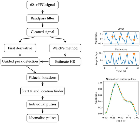
Figure 1.
Diagram overview of the signal processing steps required to extract individual pulses from the original 60 s of rPPG signal. The stars indicate the fiducial described in Section 2.2.
2.3. Training and Test Data Construction
To avoid subject leakage between the training and test set, the two datasets described in Section 2.1 were kept strictly separate, with the larger Vision-MD dataset used for training and the smaller laboratory dataset reserved for testing. For the training set, 2500 individual pulses were randomly sampled, with the constraint that each participant contributed at least one pulse. An equivalent sampling strategy was applied to the test set, from which 400 individual pulses were selected.
2.4. Human Signal Quality Labelling
In order to facilitate human scoring of individual pulse plausibility, a dedicated graphical user interface was developed in Python 3.9, as shown in Figure 2. This user interface had the following features:
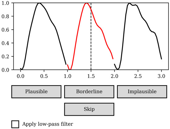
Figure 2.
Image of the UI used to assess individual pulses, showing a plausible pulse under assessment (in red) with a preceding and succeeding pulse on either side.
- Random selection of individual pulses from the training and test set (as described in Section 2.3).
- Highlighted presentation of the individual pulse to be scored in the context of its immediate predecessor and successor taken from the contiguous pre-processed signal. A vertical line was present in the middle of the pulse under assessment to visualise the plausibility of peak locations.
- The ability to select a low-pass filtered version of the 3 pulses in the assessment window. This was included to facilitate the visual identification of broad morphological features while removing the high-frequency noise often present in rPPG signals, which can otherwise obscure the identification of salient features.
- Clickable buttons to select from three choices to rate the plausibility of the highlighted pulse, plausible, borderline, or implausible, with an additional button to skip assessment in cases of too much uncertainty.
The skip option was only used if the assessor was unable to make an assessment, for example, when the pulse under assessment seemed plausible but the neighbouring pulses were excessively noisy and didn’t allow for a comparison of morphology between the three sequential pulses. Wrongly labelled pulses could significantly impact the model’s performance and avoiding mislabelling is more important than increasing the dataset size [26]. Once one of the buttons had been clicked, all buttons were disabled for 2 s. This was introduced to give a short mental rest to prevent the assessor from making a hasty judgement of the next pulse and to avoid accidental double clicks leading to mislabelled pulses.
The three assessors all had multiple years of research experience working with either remote or contact PPG signals from human subjects and adopted a holistic approach to pulse plausibility scoring, with attention to the following morphological characteristics:
- Symmetry/skewness. In common with invasive recordings of central blood pressure waveforms, valid pulses recorded from PPG signals usually have a faster systolic rise than diastolic decay. Skewness has previously been found to be a key PPG signal quality parameter [16].
- A distinct systolic peak before the halfway time point of the pulse, visualised by the vertical dashed line in the user interface.
- Presence of one or more inflection points during the diastolic decay following the systolic peak. A true dicrotic notch is not often visible in rPPG pulses, possibly due to the local haemodynamics of the microvasculature combined with the fact that green light wavelengths only penetrate the capillaries in the top 1 mm of the dermis [27].
- Morphological similarity to the immediate predecessor and successor of the pulse under assessment. This did not mean that all three pulses had to be identical, but they had to possess a similar systolic rise shape and the presence of diastolic inflection points in similar locations relative to the start and end of the pulses.
- Absence of spikes, troughs, and other gross signal disturbances when the optional low-pass filter was applied.
Pulses scored as borderline had most, but not all of the above characteristics and pulses scored as implausible had few or none of these characteristics. One assessor scored the entirety of the training set, whilst the other two assessors independently scored the entire test set. Where one of the test set pulses was scored differently between the two assessors, the third assessor was brought in to adjudicate and reach a consensus on a single score for that pulse. Examples of pulses scored in the three categories meeting these criteria can be seen in Figure 3.
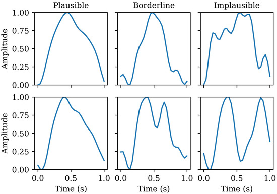
Figure 3.
Examples of plausible, borderline, and implausible individual pulses.
2.5. Model Training
Once the individual pulses were labelled, we formulated three main classification tasks:
- A three-class classification task (plausible vs. borderline vs. implausible)
- Three pairwise binary classification tasks (plausible vs. borderline; plausible vs. implausible; borderline vs. implausible) to quantify separability between categories.
- A binary classification task where borderline and implausible pulses are combined into one category (plausible vs. noise corrupted pulses)
2.5.1. Model Selection and Hyperparameter Optimization
All models used were multilayer perceptron classifiers (MLPCs). The model inputs were normalised individual pulses represented as one-dimensional arrays. Hyperparameter optimisation was performed using scikit-learn’s GridSearchCV, which conducts an exhaustive search over a predefined parameter grid, shown in Table 1, while incorporating cross-validation. In total, 504 hyperparameter combinations were evaluated for each classification task.

Table 1.
Table with hyperparameters used in grid search for model fine-tuning.
GridSearchCV systematically tests every possible combination of hyperparameter values, training and validating each configuration using stratified 5-fold cross-validation (80/20 split per fold). Model selection was based on macro-recall, and the final model for each task was retrained on the full training dataset using the best-performing hyperparameters.
2.5.2. Data-Scaling Study
To quantify data efficiency, performance was tracked as a function of training-set size. For each task, we incrementally increased the number of training samples (in steps of 100 pulses) with an 80/20 split applied for validation at each step. Thus, for a given size N, models were trained on 80% of the data (e.g., 80, 160, 240 samples) and validated on the remaining 20% (20, 40, 60 samples, respectively). The optimal hyperparameters identified from the grid search on the full training set were fixed and reused for all subsets. Learning curves were generated to evaluate whether performance approached a plateau, thereby indicating that the available training set was sufficiently large to generalise to unseen data without needing a larger training set.
2.5.3. Performance Evaluation
Model performance was assessed primarily using recall, precision, and , reported separately for each class. Recall and precision are defined as follows:
where is the number of true positives, i.e., pulses correctly classified in that category, the number of false positives, i.e., pulses incorrectly assigned to that category, and the number of false negatives, i.e., pulses belonging to that category but missed by the classifier. can be calculated using precision and recall as follows:
In addition, confusion matrices were generated to visualise misclassification patterns across classes for the three-class classification task. To provide a single aggregated measure of performance across classes, we also reported the macro-averaged score, which accounts for both precision and recall while weighting each class equally as shown in Equation (4), where C is the number of classes.
For the pairwise binary classification task, separability of the different categories was quantified using the area under the receiver operating characteristic curve (ROC-AUC), which indicates how well the classifier distinguishes between the two categories. In addition, confusion matrices and recall scores are reported for each category. Due to the differences in numbers between the categories, the macro-weighted -score is reported in this case, which not only balances the classes but also the number of samples in each class as shown in Equation (5), where C is the number of classes, the support of class i, i.e., the number of pulses in class i, and N the total number of pulses between the two classes in the pairwise binary classifier.
For the final binary classification task, recall, precision, and are reported and a confusion matrix is used to visualise the performance.
2.5.4. Usability Evaluation
In addition to classification performance metrics, the impact of the proposed pulse selection method on usability was also assessed. In previous iterations of Lifelight’s blood pressure algorithm a signal was only considered usable if more than 10 pulses in an individual signal were clustered using agglomerative clustering [18]. Agglomerative clustering is a hierarchical algorithm that groups pulses by iteratively merging the most similar pairs into clusters [28]. Although this algorithm was successful in terms of creating an average representation of the waveform with a reduced noise contribution, it also potentially removes physiologically plausible variation in the morphology. In this work, a usable signal is redefined as any individual measurement that has more than 10 plausible pulses that could be used to create an average waveform, with the aims to increase both usability and accuracy. To understand the impact on usability, a direct comparison is made between the proportion of signals meeting the usability criterion under the agglomerative clustering approach and the automated labelling approach within the Vision-MD dataset.
3. Results
3.1. Dataset Summary
In the training set, 2366 were labelled as either plausible, borderline, or implausible. The other 134 pulses were skipped by the observer, most frequently due to significant noise in the neighbouring pulses, making it difficult to judge the plausibility of the pulse under assessment. In the test set, 394 pulses were labelled as either plausible, borderline or implausible and 18 pulses needed to be discussed by all three observers to reach agreement on the score. In Table 2, an overview of the diversity in each of the datasets is shown.

Table 2.
Overview of subject distribution in training and test dataset.
Table 3 shows the distribution of plausible, borderline, and implausible pulses in both datasets. Notably, the percentage of plausible pulses is higher in the test set. This is likely due to the controlled data capture process in the clinical laboratory study, with improved lighting conditions. While the training dataset exhibits a moderate class imbalance; corrective measures such as resampling or class weighting were not employed, as the distribution reflects real-world conditions, and model performance (described in the next section) was not adversely affected.

Table 3.
Overview of the pulse label distribution in training and test dataset.
3.2. Three-Class Classifier Performance
The best performing hyperparameters and corresponding macro recall for the three-class classifier are listed in Table 4. The performance of the three-class MLP classifier was examined as a function of training set size using 80/20 validation, as shown in Figure 4. Recall for the plausible and implausible categories increases rapidly, reaching a stable plateau within the training dataset size. The borderline category also plateaus but does not reach the same level of confidence in recall. The confusion matrix on the test data supports this finding, as shown in Figure 5. Most misclassifications involved borderline pulses being assigned to either plausible or implausible, whereas confusion between plausible and implausible was less common.

Table 4.
Best performing hyperparameters for each task. Reported recall is averaged over five-fold cross validation within Vision-MD dataset.
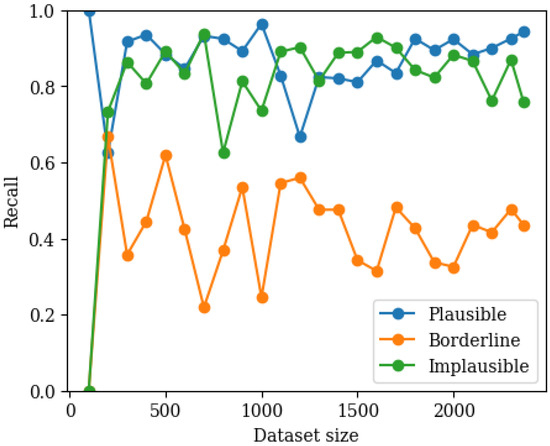
Figure 4.
Graph showing recall for each class as a function of training set size (80/20 validation) in the three-class classifier.
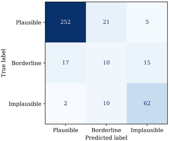
Figure 5.
Confusion matrix on the withheld test set, illustrating more frequent misclassification of borderline signals as plausible or implausible.
Table 5 shows the precision, recall, and -score per class. The macro-averaged was 0.65, reflecting the lower recall and precision on the borderline pulses, while performance for both the plausible and implausible category was significantly better.

Table 5.
Table overview of precision, recall, -score, and support (the number of pulses in the test set in this category), along with the macro-averaged -score, for the three-class MLPC on the withheld test set.
3.3. Pairwise Binary Classifier Results
The best performing hyperparameters and corresponding macro recalls for the three pairwise binary classifiers are listed in Table 4. Similar to the analysis for the three-class classifier, performance for each of the pairwise classifiers was examined as a function of training set size using 80/20 validation, as shown in Figure 6. It can be seen that in all three binary classifiers, the dataset size is large enough for the performance to stabilise. It can also be seen that some categories appear to have a better separability; the recall between plausible and implausible is higher than the recall between plausible and borderline. To fully understand the separability between the three categories, the macro-weighted and ROC-AUC are compared.
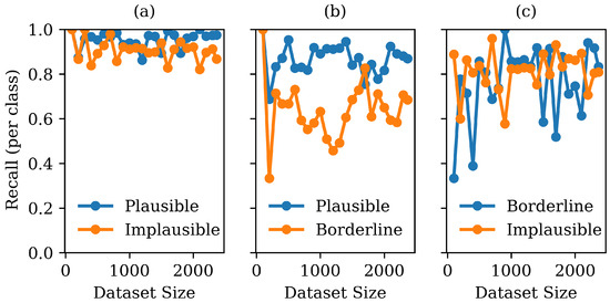
Figure 6.
Graph showing recall for each class as a function of training set size (80/20 validation) in the pairwise classifiers: (a) plausible vs. implausible; (b) plausible vs. borderline; and (c) borderline vs. implausible.
Table 6 shows -scores and macro-averaged -scores for each of the pairwise binary classifiers. It can be seen that, while the -scores are lowest for the borderline category, overall the performance between plausible and implausible against borderline is similar, indicating that the model can distinguish between plausible, borderline, and implausible signals in all cases and that borderline cases should not be considered as either plausible or implausible without further investigation. Figure 7 shows that all three curves lie well above the chance curve, confirming strong separability between all category pairs.

Table 6.
Per-class and macro-weighted -scores for each pairwise binary classifier.
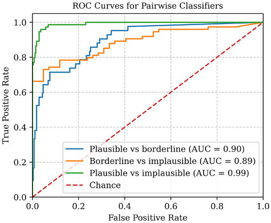
Figure 7.
ROC curves for the three pairwise binary classifiers, each showing high separability between categories with ROC–AUC values > 0.89.
3.4. Plausible vs. Borderline and Implausible Combined
The best performing hyperparameters for the binary classifier between plausible and noise corrupted (implausible and borderline combined) pulses are show in Table 4. In Figure 8, the performance of the classifier as a function of training set size using 80/20 validation is shown. It can be seen that the recall for both categories stabilises within the training dataset size and that both categories have a good recall.
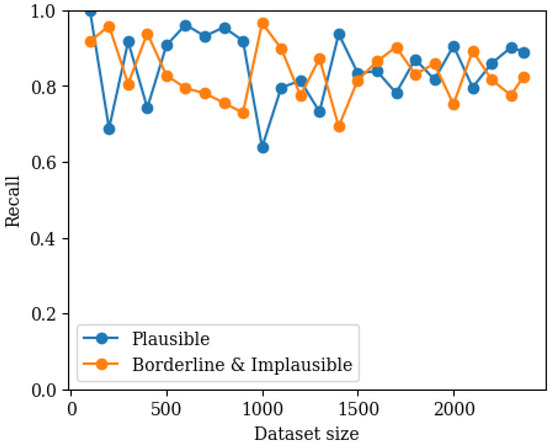
Figure 8.
Graph showing recall for both classes as a function of training set size (80/20 validation) in the binary classifier where implausible and borderline pulses have been combined into one category.
Figure 9 shows the confusion matrix of the binary classifier on the withheld test set. It can be concluded that the recall for the plausible category is 92%, the precision 94%, and therefore the -score 0.93, showing that the classifier performs robustly on detecting the relevant plausible pulse category, with few false positives or false negatives, supporting the practical implementation of automated signal quality control.
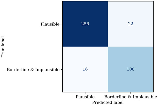
Figure 9.
Confusion matrix on the withheld test set using the binary classifier where implausible and borderline pulses have been combined into one category.
3.5. Usability Results
Using the agglomerative clustering method, the number of usable pulses within a signal was often limited, because only self-similar pulses were retained. Within the Vision-MD dataset described in Section 2.1, more than 42% of the signals did not have enough clustered pulses to be used for blood pressure prediction. The automated labelling method retains all plausible pulses, leading to a significant increase in usable pulses for each signal; only 5% of the signals do not meet the criteria of having more than 10 pulses. Figure 10 shows the distribution of usable pulse counts for each method. This histogram demonstrates that automated labelling results in higher counts of usable pulses per signal compared to agglomerative clustering, suggesting that automated labelling may allow more data to be retained for subsequent analysis.
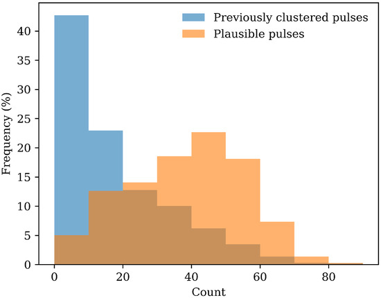
Figure 10.
Histogram of the number of usable pulses per signal under the agglomerative clustering method and automated labelling method.
4. Discussion
This study investigated the automation of labelling individual rPPG pulses as plausible, borderline or implausible using MLPCs trained on human annotations. The initial three-class classifier achieved good overall performance, but recall on borderline pulses compared to plausible and implausible pulses was notably lower. To explore whether this reflected an overlap between classes, three different pairwise binary classifiers were trained and analysed, to study whether the three classes were independently separable, or if the borderline category should be merged with either the plausible or implausible category. The consistently high ROC–AUC values (>0.89) across all binary comparisons indicate that plausible, borderline, and implausible pulses are, in fact, distinguishable, and therefore the borderline label captures a meaningful and independent category rather than a subset of the others. However, from a deployment standpoint, a pulse is either usable or not usable, which supports the consideration of collapsing borderline and implausible into a single class. This simplifies the model required and improves robustness to disagreements at the implausible–borderline boundary. In this binary model, the plausible vs. implausible and borderline classifier achieves and -score of 0.93.
Despite the promising results, some limitations should be noted. First, the training labels relied on human scoring, which can be fallible, particularly for borderline pulses where subjective judgement can be more variable. This subjectivity introduces a level of uncertainty into the ground truth human labels and may contribute to the lower recall observed in this category in the three-class classifier. Secondly, the skipping of pulses without a clear relation to the (often too noisy) neighbouring pulses may inadvertently exclude less common but physiologically valid morphologies. These limitations could be overcome in future work by using more data, aiming for a more equally distributed training dataset or a wider range of categories (e.g. plausible, borderline–plausible, uncertain, borderline–implausible, implausible). One way of implementing more detailed categories without relabelling the training set could be to incorporate classifier probability outputs rather than discrete labels. This would allow uncertainty to be expressed directly, distinguishing borderline–plausible from borderline–implausible. Alternatively, fuzzy divergence approaches could be explored to represent pulses with graded membership across categories, providing a formal framework for modelling ambiguity in borderline cases.
Using a much larger dataset, another potential workaround for the limitation in borderline pulses detection could be to include more than one pulse, or even the full signal, into the algorithm for consideration of an individual pulse’s plausibility within the context of the variability and morphologies seen within an individual’s measurement.
One of the potential implementations of the automated pulse labelling algorithm could be within a pulse clustering framework. Previous approaches relied on ensemble averaging, where the largest cluster of self-similar pulses was used to represent morphology [18,28]. In contrast, the proposed method enables averaging across all plausible pulses, thereby capturing the true underlying morphology while preserving physiological variability that would otherwise be discarded. This not only has the potential to improve accuracy in blood pressure prediction, but also to improve usability (Section 3.5). Additionally, if individual pulse quality can be assessed in real time, measurements could be stopped as soon as a sufficient number of plausible pulses are collected, enabling faster results without compromising reliability.
In this proof-of-concept study, the focus was deliberately on MLPC because they offer a computationally efficient solution to evaluate the feasibility of automated pulse quality assessment. An important avenue for future work would be to explore approaches that improve classification performance in challenging or ambiguous cases, particularly those currently assigned to the borderline category. This work could include investigating alternative model architectures, such as convolutional neural networks (CNNs), recurrent models (e.g., LSTMs) or transformer-based architectures, which might be capable of capturing more complex dependencies in the signals. In parallel, enhancing data preprocessing and cleaning strategies could provide the model with higher-quality input pulses for classification. Such enhancements may lead to a more robust recall of borderline cases and improve the performance of downstream applications.
Future work should also investigate the generalisability of this approach to different populations, specifically paediatric patients. In the present study, data collection was limited to adults over 18 years old, but it remains to be seen whether the same labelling strategy is valid in children, whose rPPG signal characteristics may differ substantially due to the differences in vital signs such as faster pulse and respiration rates. Moreover, testing the algorithm in patients with arrhythmias such as atrial fibrillation could be valuable. It could be challenging due to the changes in amplitude and shape in irregular heartbeats [29], which may require additional training data and model training to identify which pulses are plausible. If the algorithm were able to identify plausible pulses even in the presence of irregular heart rhythms this could support blood pressure prediction in cases that could be challenging for the previously used ensembling approach.
5. Conclusions
This work presents automated pulse quality labelling as a key step towards more robust rPPG vital sign processing, with the aims of improving accuracy and usability. On a separate test set (394 pulses from 58 participants), the three-class MLPC achieved a macro-averaged -score of 0.65 with per-class recall of 91%, 24% and 84% for plausible, borderline and implausible pulses respectively. When considering borderline and implausible pulses as a single not usable class, the binary classifier between plausible and noise corrupted pulses achieved an -score of 0.93 on the same test set. The proportion of signals with enough usable pulses increased from 58% with agglomerative clustering to 95% with automated labelling.
These findings suggest that learning pulse plausibility directly from the individual pulse, without additional feature extraction, could be used to select pulses for more stable and accurate downstream vital-sign (such as BP) estimates from rPPG signals.
Author Contributions
Conceptualization, L.D.v.P.; methodology, L.D.v.P. and S.W.; software, L.D.v.P.; validation, L.D.v.P.; formal analysis, L.D.v.P.; investigation, A.J.W.M., L.D.v.P. and S.W.; data curation, L.D.v.P.; writing—original draft preparation, L.D.v.P.; writing—review and editing, S.W.; visualization, L.D.v.P.; supervision, S.W. All authors have read and agreed to the published version of the manuscript.
Funding
The data collection of the vision-MD dataset was funded by a National Institute for Health and Care Research (NIHR) Artificial Intelligence Award (AI award 02031). This report is an independent research funded by the NIHR and National Health Service user experience (NHSX), now part of NHS England. The views expressed in this publication are those of the authors and not necessarily those of the NIHR, NHSX, or Department of Health and Social Care.
Institutional Review Board Statement
The data collection protocol for the VISION-MD study was approved by the South Berkshire Research Ethics Committee. Before the study started, the initial study protocol was approved by Health Research Authority (HRA) Wales. HRA Wales has also approved subsequent protocol amendments. The data collection protocol for the clinical laboratory study was approved by Salus Institutional Review Board, Austin, TX, USA. All data collection was performed in accordance with the Declaration of Helsinki.
Informed Consent Statement
Informed consent was obtained from all subjects involved in the study.
Data Availability Statement
The data sets generated during and/or analysed during the current study are not publicly available due to the commercial sensitivity of these data, which is mandated in Xim’s contractual obligations with the National Institute for Health Research (NIHR) and National Health Service user experience (NHSX), which funded this research. Moreover, the informed consent provided by study participants was made on the basis that only authorised individuals of the research team based at the study sites (Xim and Xim’s authorised partners) would have access to their data, even in anonymised form. Excluding other reasons for data access, the study data are available from the corresponding author upon reasonable request.
Acknowledgments
We thank all staff and participants at Barts Health NHS Trust and Portsmouth Hospitals University Trust for their involvement in the Vision-MD study. We are also grateful to the team at Element (formerly Clinimark) for their assistance with clinical laboratory data collection. Finally, we would like to thank the research team at Xim Ltd. for their valuable insights and contributions to project discussions.
Conflicts of Interest
All authors are employed by Xim Ltd. Authors declare that the research was conducted in the absence of any commercial or financial relationships that could be construed as a potential conflict of interest.
Abbreviations
The following abbreviations are used in this manuscript:
| BP | Blood pressure |
| HR | Heart rate |
| MLPC | MultiLayer Perceptron Classifier |
| PPG | Photoplethysmography |
| PSD | Power Spectral Density |
| rPPG | remote Photoplethysmography |
| ROC-AUC | Receiver Operating Characteristic-Area Under the Curve |
| SNR | Signal to Noise Ratio |
| SQI | Signal Quality Index |
References
- Elgendi, M.; Fletcher, R.; Liang, Y.; Howard, N.; Lovell, N.H.; Abbott, D.; Lim, K.; Ward, R. The use of photoplethysmography for assessing hypertension. NPJ Digit. Med. 2019, 2, 60. [Google Scholar] [CrossRef]
- Verkruysse, W.; Svaasand, L.O.; Nelson, J.S. Remote plethysmographic imaging using ambient light. Opt. Express 2008, 16, 21434–21445. [Google Scholar] [CrossRef]
- Almarshad, M.A.; Islam, M.S.; Al-Ahmadi, S.; BaHammam, A.S. Diagnostic features and potential applications of PPG signal in healthcare: A systematic review. Healthcare 2022, 10, 547. [Google Scholar] [CrossRef]
- Zhang, C.; Jovanov, E.; Liao, H.; Zhang, Y.T.; Lo, B.; Zhang, Y.; Guan, C. Video based cocktail causal container for blood pressure classification and blood glucose prediction. IEEE J. Biomed. Health Inform. 2022, 27, 1118–1128. [Google Scholar] [CrossRef]
- van Putten, L.D.; Bamford, K.E. Improving systolic blood pressure prediction from remote photoplethysmography using a stacked ensemble regressor. In Proceedings of the IEEE/CVF Conference on Computer Vision and Pattern Recognition, Vancouver, BC, Canada, 17–24 June 2023; pp. 5957–5964. [Google Scholar]
- Elgendi, M.; Haugg, F.; Fletcher, R.R.; Allen, J.; Shin, H.; Alian, A.; Menon, C. Recommendations for evaluating photoplethysmography-based algorithms for blood pressure assessment. Commun. Med. 2024, 4, 140. [Google Scholar] [CrossRef]
- Gupta, S.S.; Kwon, T.H.; Hossain, S.; Kim, K.D. Towards non-invasive blood glucose measurement using machine learning: An all-purpose PPG system design. Biomed. Signal Process. Control 2021, 68, 102706. [Google Scholar]
- Dixon, B.; Sharkey, J.M.; Teo, E.J.; Grace, S.A.; Savage, J.S.; Udy, A.; Smith, P.; Hellerstedt, J.; Santamaria, J.D. Assessment of a non-invasive brain pulse monitor to measure intra-cranial pressure following acute brain injury. Med. Devices Evid. Res. 2023, 16, 15–26. [Google Scholar] [CrossRef] [PubMed]
- Bradley, G.R.; Kyriacou, P.A. Exploring the dynamic relationship: Changes in photoplethysmography features corresponding to intracranial pressure variations. Biomed. Signal Process. Control 2024, 98, 106759. [Google Scholar] [CrossRef]
- Lu, Y.; Wang, C.; Meng, M.Q.H. Video-based Contactless Blood Pressure Estimation: A Review. In Proceedings of the 2020 IEEE International Conference on Real-time Computing and Robotics (RCAR), Asahikawa, Japan, 28–29 September 2020; pp. 62–67. [Google Scholar] [CrossRef]
- Rohmetra, H.; Raghunath, N.; Narang, P.; Chamola, V.; Guizani, M.; Lakkaniga, N.R. AI-enabled remote monitoring of vital signs for COVID-19: Methods, prospects and challenges. Computing 2021, 105, 783–809. [Google Scholar] [CrossRef]
- Desquins, T.; Bousefsaf, F.; Pruski, A.; Maaoui, C. A Survey of Photoplethysmography and Imaging Photoplethysmography Quality Assessment Methods. Appl. Sci. 2022, 12, 9582. [Google Scholar] [CrossRef]
- Charlton, P.H.; Marozas, V.; Mejía-Mejía, E.; Kyriacou, P.A.; Mant, J. Determinants of photoplethysmography signal quality at the wrist. PLoS Digit. Health 2025, 4, e0000585. [Google Scholar] [CrossRef]
- Karlen, W.; Kobayashi, K.; Ansermino, J.M.; Dumont, G.A. Photoplethysmogram signal quality estimation using repeated Gaussian filters and cross-correlation. Physiol. Meas. 2012, 33, 1617. [Google Scholar] [CrossRef]
- Orphanidou, C.; Bonnici, T.; Charlton, P.; Clifton, D.; Vallance, D.; Tarassenko, L. Signal-quality indices for the electrocardiogram and photoplethysmogram: Derivation and applications to wireless monitoring. IEEE J. Biomed. Health Inform. 2014, 19, 832–838. [Google Scholar] [CrossRef]
- Elgendi, M. Optimal signal quality index for photoplethysmogram signals. Bioengineering 2016, 3, 21. [Google Scholar] [CrossRef]
- Wiffen, L.; Brown, T.; Maczka, A.B.; Kapoor, M.; Pearce, L.; Chauhan, M.; Chauhan, A.J.; Saxena, M.; Group, L.T. Measurement of vital signs by lifelight software in comparison to standard of care multisite development (VISION-MD): Protocol for an observational study. JMIR Res. Protoc. 2023, 12, e41533. [Google Scholar] [CrossRef] [PubMed]
- van Putten, L.D.; Bamford, K.E.; Veleslavov, I.; Wegerif, S. From video to vital signs: Using personal device cameras to measure pulse rate and predict blood pressure using explainable AI. Discov. Appl. Sci. 2024, 6, 184. [Google Scholar] [CrossRef]
- Lempe, G.; Zaunseder, S.; Wirthgen, T.; Zipser, S.; Malberg, H. ROI selection for remote photoplethysmography. In Proceedings of the Bildverarbeitung für die Medizin 2013: Algorithmen-Systeme-Anwendungen Workshop, Heidelberg, Germany, 3–5 March 2013; Springer: Berlin/Heidelberg, Germany, 2013; pp. 99–103. [Google Scholar]
- Hufschmidt, K.; Camuzard, O.; Balaguer, T.; Baqué, P.; de Peretti, F.; Santini, J.; Bronsard, N.; Qassemyar, Q. The infraorbital artery: From descriptive anatomy to mucosal perforator flap design. Head Neck 2019, 41, 2065–2073. [Google Scholar] [CrossRef]
- Wang, W.; Den Brinker, A.C.; Stuijk, S.; De Haan, G. Algorithmic principles of remote PPG. IEEE Trans. Biomed. Eng. 2016, 64, 1479–1491. [Google Scholar] [CrossRef] [PubMed]
- Miller, D.J.; Sargent, C.; Roach, G.D. A validation of six wearable devices for estimating sleep, heart rate and heart rate variability in healthy adults. Sensors 2022, 22, 6317. [Google Scholar] [CrossRef]
- Peralta, E.; Lazaro, J.; Bailon, R.; Marozas, V.; Gil, E. Optimal fiducial points for pulse rate variability analysis from forehead and finger photoplethysmographic signals. Physiol. Meas. 2019, 40, 025007. [Google Scholar] [CrossRef]
- Solomon, O.M., Jr. PSD Computations Using Welch’s Method; Power Spectral Density (PSD); Sandia National Laboratories: Albuquerque, NM, USA, 1991. [CrossRef]
- Wegerif, S.; Veleslavov, I.; Van Putten, L.D.; Bamford, K.E.; Misra, G.; Mullen, N. Paediatric Pulse Rate Measurements: A Comparison of Methods using Remote Photoplethysmography. In Proceedings of the IEEE/CVF Conference on Computer Vision and Pattern Recognition, Seattle, WA, USA, 17–21 June 2024; pp. 364–370. [Google Scholar]
- Ding, C.; Pereira, T.; Xiao, R.; Lee, R.J.; Hu, X. Impact of Label Noise on the Learning Based Models for a Binary Classification of Physiological Signal. Sensors 2022, 22, 7166. [Google Scholar] [CrossRef] [PubMed]
- Volkov, M.V.; Margaryants, N.B.; Potemkin, A.V.; Volynsky, M.A.; Gurov, I.P.; Mamontov, O.V.; Kamshilin, A.A. Video capillaroscopy clarifies mechanism of the photoplethysmographic waveform appearance. Sci. Rep. 2017, 7, 13298. [Google Scholar] [CrossRef] [PubMed]
- Waugh, W.; Allen, J.; Wightman, J.; Sims, A.J.; Beale, T.A. Novel signal noise reduction method through cluster analysis, applied to photoplethysmography. Comput. Math. Methods Med. 2018, 2018, 6812404. [Google Scholar] [CrossRef]
- Sološenko, A.; Petrėnas, A.; Marozas, V.; Sörnmo, L. Modeling of the photoplethysmogram during atrial fibrillation. Comput. Biol. Med. 2017, 81, 130–138. [Google Scholar] [CrossRef] [PubMed]
Disclaimer/Publisher’s Note: The statements, opinions and data contained in all publications are solely those of the individual author(s) and contributor(s) and not of MDPI and/or the editor(s). MDPI and/or the editor(s) disclaim responsibility for any injury to people or property resulting from any ideas, methods, instructions or products referred to in the content. |
© 2025 by the authors. Licensee MDPI, Basel, Switzerland. This article is an open access article distributed under the terms and conditions of the Creative Commons Attribution (CC BY) license (https://creativecommons.org/licenses/by/4.0/).