Article

Statistical Modeling and Analysis of Similar Compound Interaction in Scientific Research

by
Timothy E. O’Brien
Department of Mathematics and Statistics, Loyola University Chicago, Chicago, IL 60202, USA
Appl. Sci. 2025, 15(18), 9971; https://doi.org/10.3390/app15189971
Submission received: 9 August 2025 / Revised: 9 September 2025 / Accepted: 9 September 2025 / Published: 11 September 2025
(This article belongs to the Special Issue Exposure Pathways and Health Implications of Environmental Chemicals)

Abstract

In many practical scientific studies, two-way analysis of variance (ANOVA) and linear response surface methods are used for determining whether two or more similar compounds (substances, agents, or drugs) interact synergistically, antagonistically or independently. These models are often found lacking both in the means to assess interaction and with sufficient power. Using ten judiciously chosen illustrations (spanning fields as diverse as aquatic and environmental toxicology, botany, entomology, oncology, pharmacology, and virology), this paper introduces, explores, quantifies, illustrates, interprets, and extends several cutting-edge nonlinear assessment models and methods for measuring and describing interaction. Developed and used here are the Finney and Separate Ray models and extensions, a new cut line approach useful for so-called web designs, and extensions to more than two substances. As noted in the provided examples, the Finney model and extensions have the advantage of characterizing nonlinear interaction in a single measure, whereas the Separate Ray model extension is required when nonlinear interaction requires more than a single parameter for interaction assessment. The interaction results of the ten illustrations—of which antagonism is observed in four examples, synergy in five examples, and mixed results in one example—are summarized below. A discussion is also provided of efficient experimental design strategies as an aid to the practitioner and their future scientific studies.

1. Introduction

The assessment of interaction is paramount in scientific studies including work in agricultural, chemical, environmental, health/biomedical, and other fields of research. Historically, these assessments have largely been carried out using statistical methods including linear regression with interaction terms, two-way ANOVA, and/or linear response surface techniques; see, e.g., [1,2,3,4]. Such linear models often lack sufficient power to detect interaction in practical applications since they often have too few design support points to efficiently estimate the interaction term. For example, in [1], the interaction of ozone (O3) and sulfur dioxide (SO2) is assessed using a two-way ANOVA model and an experimental design which only includes the four factorial runs of (a) both O3 and SO2 absent, (b) O3 absent and SO2 present, (c) O3 present and SO2 absent, and (d) both O3 and SO2 present. More detailed information can be discerned when the design includes cross-combinations of, say, 0.03, 0.05, 0.07, 0.09 and 0.11 ppm of O3 and 65, 75 and 85 ppb of SO2 in a 5 × 3 factorial study. This follows since the minimal interaction linear model, y = β 0 + β 1 x 1 + β 2 x 2 + β 12 x 1 x 2 + e (which would have more terms if quadratic effects were included), has four model function parameters plus the variance. So, with only four support points but five model parameters, the 2 × 2 used in [1] factorial lacks sufficient power to efficiently estimate all model terms (especially lack-of-fit). We also underscore that the precise manner of obtaining such interaction information is also important. To illustrate, Refs. [2,4] use linear regression-type models or response surface methods (see [5,6]). These linear methods can also lack power when the constituent effects interact in a curved manner, and nonlinear models have often been successfully used; see Refs. [7,8,9,10,11,12,13,14,15,16,17,18,19,20,21,22,23,24,25,26,27,28,29,30,31,32,33,34,35,36,37,38,39,40] which underscore the need for and usefulness of these nonlinear assessments and Ref. [19] (p. 365) which explores power assessments of various linear and nonlinear models using Monte-Carlo simulations.
This current work introduces and evaluates nonlinear interaction statistical models for analyzing quantitative-input-variable data and illustrates with designed experiments. Background references to nonlinear and bioassay modeling include [41,42,43,44,45,46,47,48,49]. The interaction models we propose here build upon these basic nonlinear models, and some additional details on nonlinear interaction models are provided in [50,51,52,53,54,55,56,57]. Mindful that a few definitions exist for assessing synergy and antagonism (see [58,59]), we underscore that the focus here is solely on the popular Loewe interaction (also called concentration additivity) which uses the isobole and separate ray approaches discussed in Section 2, Section 3 and Section 4; the term ‘isobole’ is introduced and discussed in [60]. In contrast, the Bliss approach and characterization of independent action (no interaction) uses a probabilistic perspective as detailed and discussed in [58]. Our choice of the Loewe approach follows recommendations from several authors including [61,62]. Ref. [61] highlights that the Loewe interaction model is expected to be accurate when two compounds have the same mechanism of action or pathway, and the Bliss model applies when the factors have different mechanisms of action and do not directly interact but nonetheless amplify or inhibit one another. Ref. [62] refutes this claim, stating that both methods can be used for mixtures with dissimilar modes of action, and further state that the Bliss approach is based on assumptions rarely met in practice.
Nonlinear interaction models are exemplified, explored and discussed here as follows. The basic Finney model and its extensions are introduced and illustrated in Section 2. After discussing some potential shortcomings of the Finney model, in Section 3 we introduce and illustrate the Separate Ray model and give key extensions. Several additional important applications are presented and discussed in Section 4 including our cut-line approach to assessing interaction for web designs. Finally, in Section 5, we summarize our results and give comments regarding experimental design strategies and additional extensions. To solidify and illustrate the methods we introduce and discuss here, this work includes ten carefully chosen examples of increasing complexity and breadth. In sum, this work develops, extends and illustrates the Finney interaction models (with extensions), the Separate Ray models (which are required when the Finney models show significant lack-of-fit), and provide key adaptations for non-normal and non-binomial responses, random effects, assessments for web-designs, and for studies involving three or more factors.

2. Nonlinear Assessment of Interaction: The Finney Model and Extensions

An important model which has been proposed to statistically represent interacting mechanisms and to allow for the assessment of statistical interaction is the Finney model (see [8]). For quantitative response data, down-sloping responses, and two explanatory variables (i.e., agents, compounds, pollutants, drugs, etc.) this model employs the so-called Finney5 model function,
E y = η x 1 , x 2 = θ 1 1 + z / θ 2 θ 3 ,   z = x 1 + θ 4 x 2 + θ 5 θ 4 x 1 x 2                    
Note that the ‘5’ used here in the ‘Finney5’ title refers to the number of model function parameters. In this expression, y is the quantitative response variable, x 1 0 is the amount of the first agent, x 2 0 is the amount of the second agent, and z is called the effective dose since it represents the combined dose received by the experimental unit. In this five-parameter model function, θ 1 is the expected response for x 1 = x 2 = 0 , so it can be viewed as the baseline or negative control hypothesized (or expected) response. Sometimes called the E C 50 ,   E D 50 , I C 50 , or L D 50 parameter for the x 1 variable (where ‘C’ stands for concentration and ‘D’ for dose), θ 2 is such that η ( θ 2 , 0 ) = θ 1 / 2 . So it is the concentration level (actually line or curve here) to achieve 50% inhibition. θ 3 is the slope parameter, so it represents how quickly the response curve increases or decreases. Also, θ 4 is the relative potency parameter of compound 2 to compound 1, meaning that in the absence of interaction if, say, θ 4 = 2 , then compound 2 is twice as potent as compound 1. Finally, θ 5 is the coefficient of synergy: whenever θ 5 does not significantly differ from zero, independent action (or no interaction) of the two agents is declared, if θ 5 is significantly positive, then synergy is observed, and if θ 5 is significantly negative, then this model indicates that the compounds behave antagonistically. This model is illustrated in Example 1 below. Note that Equation (1) simultaneously fits a nonlinear surface to the chosen two compounds. It can be fit (i.e., to obtain least-squares parameter estimates) using the NLIN procedure in SAS® (version 9.4) or the ‘nls’ function in R (version 4.5.0). As underscored in [44,63], for normal response data, maximum-likelihood and least-squares estimates (LSEs and MLEs) coincide for model parameters; only MLEs are used for non-normal response model parameters (e.g., binomial response). For variance estimation in normal models, we use here restricted MLEs employing the p-value adjustment technique for testing given in [64].
Some modifications to Equation (1) include incorporating a non-zero lower asymptote ( L A ) by using the ‘Finney6’ model function, E y = L A + θ 1 L A 1 + z / θ 2 θ 3 , or allowing the curve to slope upward from zero to θ 1 via the modified ‘Finney5b’ model function, E y = θ 1 z / θ 2 θ 3 1 + z / θ 2 θ 3 . That is, since the Finney5 model is downslope from θ 1 to zero, the Finney6 model should be used when the responses approach a non-zero ‘lower asymptote’ value ( L A , which is the expected response for very large doses). Further, the Finney5b model should be used when the data are upsloping from zero to the upper asymptote of θ 1 . Furthermore, in cases where heteroskedasticity exists, this model is easily extended to also model the variance (see Example 7 below). As noted in [44], modeling variance can be preferred to performing a transformation (such as a Box–Cox transformation). Although the response is often assumed to follow the normal distribution, this model works for other (quantitative) response variable distributions such as the Poisson or Negative Binomial distributions for count data (see Example 5 below).
In situations where a quantal response (e.g., yes/no) variable is observed one typically assumes the it follows the binomial distribution with ‘success’ probability equal to π . In this case and when the response curve is upsloping, the ‘Finney4b’ model function for compounds A and B is
π = z / θ 2 θ 3 1 + z / θ 2 θ 3 ,   z = A + θ 4 B + θ 5 θ 4 A B                      
Equation (2) simultaneously fits a nonlinear logistic surface to compounds A and B. The down-sloping ‘Finney4’ model function is π = 1 1 + z / θ 2 θ 3 . Since the response here is non-normal (i.e., binomial) and this model function is nonlinear in the parameters, the model is called a generalized nonlinear model and special algorithms are needed for parameter and interval estimation as well as for hypothesis testing. In SAS® (version 9.4), the NLMIXED and NLP procedures can be used; in R (version 4.5.0), the ‘gnm’ function provides (maximum-likelihood) parameter and interval estimates.
The following two examples illustrate the fitting and interpretations of the Finney5 model for an agricultural illustration and the Finney4 model for a toxicological example.

2.1. Example 1

In modeling the effect on cucumber seedling growth ( y ), Ref. [8] uses the Finney5 models function to estimate and test the interaction of the two phenolic acids, ferulic acid (in the amount x 1 ) and vanillic acid (in the amount x 2 ). This study has the six design support points x 1 , x 2 = 0 ,   0 ,   0 ,   0.25 ,   0 ,   0.50 ,   0.25 ,   0 , ( 0.25 ,   0.25 ) , and ( 0.50 ,   0 ) , and was performed in triplicate with one run of each of the support points run in each of three growing chambers. Assuming normality and constant variances, we fit the Finney5 model function in Equation (1), and, following [8], we allowed the upper asymptote parameters ( θ 1 s ) to vary by the three chambers (i.e., by assuming fixed chamber effects). The chosen experimental design and results are plotted in Figure 1A.
For these data, the (least-squares) model function parameter estimates are θ ^ 11 = 15.2 ,   θ ^ 12 = 13.8 ,   θ ^ 13 = 15.9 ,   θ ^ 2 = 0.19 ,   θ ^ 3 = 2.72 ,   θ ^ 4 = 0.63 , θ ^ 5 = 0.83 and the MSE is σ ^ e 2 = 3.76 . Note the substantial difference in the estimated upper asymptotes ( θ 1 s ) here for the three chambers. Further, that the coefficient of synergy estimate is negative and that its profile likelihood confidence interval (PLCI), ( 1.29 ,   0.21 ) , is completely negative (i.e., excludes zero) leads to the conclusion that this model and these data support the claim that ferulic and vanillic act antagonistically in the growth of cucumber seedlings. This follows since antagonism is detected using this model whenever the coefficient of synergy parameter ( θ 5 ) is significantly negative. Also, since θ ^ 2 = 0.19 , the E C 50 point ( 0.19 ,   0 ) appears on the horizontal (ferulic) axis in Figure 1A (filled square on the horizontal axis), and since θ ^ 2 / θ ^ 4 = 0.31 , this E C 50 point is plotted as the filled square on the vertical (vanillic) axis. Indeed, since θ ^ 4 = 0.63 , the estimated potency of vanillic to ferulic acid is a little over 62.5 % .
Instead of assuming fixed-effects upper asymptotes for the chambers (as above), we next extend the above model by assuming that the selected three chambers are taken from a random sample of such chambers and thus to treat the upper asymptotes as random effects, θ 1 ~ N ( θ 1 ,   σ 1 2 ) . That is, the realized upper asymptote for a chamber ( θ 1 ) is assumed to come from a normal distribution with true/average upper asymptote of θ 1 and with variance σ 1 2 . When this nonlinear mixed-effects model is fit to these data, the estimated experimental error σ ^ e 2 reduces from σ ^ e 2 = 3.76 to σ ^ e 2 = 0.05 . Also, the variability in the upper asymptotes is σ ^ 1 2 = 14.57 . More importantly, the updated coefficient of synergy estimate is θ ^ 5 = 0.84 , and the PLCI for θ 5 is now ( 1.16 ,   0.51 ) . This means that when the chambers are treated as random effects instead of fixed effects (above), the length of the coefficient of synergy confidence interval is cut almost in half. This occurs here due to the removal of the random intercept variability from the experimental error term and thus an increase in precision in estimating the coefficient of synergy. Regardless of which of these models is chosen, these data and the Finney5 model indicate interaction in the form of antagonism between these phenolic acids.
The next example illustrates use of the Finney4 model for quantal response data.

2.2. Example 2

Plotted in Figure 1B are the similar compound design support points of [65], which examines 20 combinations of insecticides A and B (in ppm). These A-B combinations are represented by the twenty filled circles in the plot and with ( x 1 , x 2 ) coordinates corresponding to the respective amounts of insecticides A and B. Note that the chosen design used here, a ray design with three interior rays (i.e., the non-axes lines radiating from the origin), has respective interior ray slopes of 3, 1 and 1/3. To better understand these interior rays, for a slope of c , this means that c parts of insecticide B are combined with one part of insecticide A in the treatment mixture. Thus, for example for the ray of slope 3 in Figure 1B, three parts of insecticide B are combined with every one part of insecticide A. Next, corresponding to each of the 20 A–B combinations, approximately n = 30 insects received each A–B combination and the number of dead insects ( y ) was recorded. In the data analysis, since insect mortality is observed increasing with insecticide concentration, we assume this response variable follows the binomial distribution and we fit the Finney4b model function given in Equation (2).
For these data and the Finney4b model function, the parameter estimates are θ ^ 2 = 9.95 ,   θ ^ 3 = 1.80 ,   θ ^ 4 = 0.90 and θ ^ 5 = 1.03 . The estimated E C 50 points here are 9.95 for insecticide A and 9.95 / 0.90 = 11.06 for insecticide B, so that θ ^ 4 = 0.90 is the estimated relative potency of insecticide B to A. The estimated E C 50 points are the filled squares on the vertical and horizontal axes in Figure 1B, and the estimated independent action line connects these points. The test of independent action is rejected here ( H 0 : θ 5 = 0 ,   χ 1 2 = 30.3 ,   p < 0.0001 ), meaning that the isobole in Figure 1B significantly bows outward from the estimated independent action line. As for the previous example, since the entire θ 5 PLCI here, ( 1.29 ,   0.74 ) , lies below zero, we conclude that these insecticides exhibit significant antagonism.
A deeper understanding of this model fit can be provided by examining the isobole plotted in Figure 1B. When the mortality probability values equal to 50%, so π = 1 2 , we obtain z / θ 2 = 1 so the values of A and B following the relation,
A + θ 4 B + θ 5 θ 4 A B = θ 2
Whenever θ 5 = 0 , Equation (3) is a line connecting the respective E C 50 points—this is the plotted dashed independent action line given in Figure 1B. When θ 5 0 , Equation (3) is a portion of an elliptical curve, as shown in Figure 1A,B. In general, this curve is called an isobole. The fact that this elliptical isobole curve is bowing outwards demonstrates antagonism here since all points along this curve are predicted to give 50% mortality probabilities. That is, that on this curve, when the insecticides are combined, greater amounts are needed to achieve 50% mortality. On other hand, an inward bowing isobole (which occurs if θ 5 was significantly positive as in Example 3 below) would indicate that the substances behave synergistically. Clearly in this case, insecticides A and B behave antagonistically in their effect on insect mortality.
Of note, it is useful to compare the chosen experimental designs used in Examples 1 and 2. For Example 1, the design is composed of just six design support points with five of these six points being on the single-variable axes (i.e., with at least one of the acids set equal to zero) and where only the ‘interior’ single point, (0.25, 0.25), is a true mixture point. Example 2, on the other hand, contained 12 interior (i.e., combination) support points, and the total design is composed of five rays with four support points per ray. Thus, at the very least, the design in Example 2 can certainly be used to check for the inherent model assumptions as well as model adequacy (i.e., lack of fit). Additional comments on experimental design strategies are given below in Section 5 and in [66].
We also underscore that goodness of fit of the assumed normal and binomial distributions and the assumed model functions for Examples 1 and 2 can and should be assessed by plotting the model residuals versus the fitted values; these distributional and model fits are supported by the respective residual plots (not displayed here).
The following example illustrates another important extension of the Finney model.

2.3. Example 3

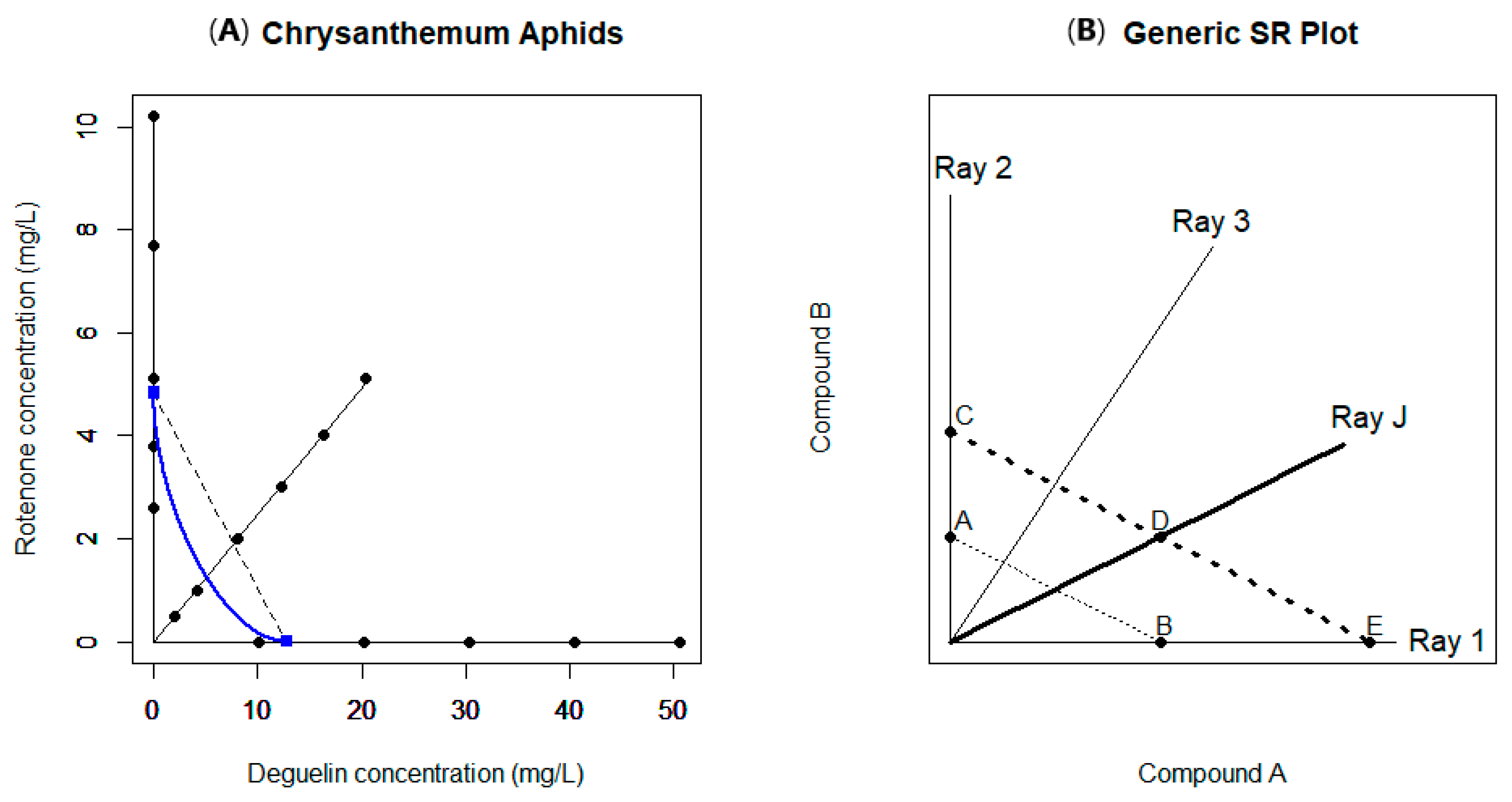
Employing a ray design with a single interior ray, Ref. [67] studied the effect of the insecticides deguelin ( x 1 ) and rotenone ( x 2 ) in isolation and in a 1:4 (rotenone-to-deguelin) mixture. The chosen number of support points on the deguelin ( x 1 ) and the rotenone ( x 2 ) axes were five and the number on the interior ray was six; following [13,67] and others, we omit data from a first deguelin-only support point. For each of the 16 support points approximately n = 50 chrysanthemum aphids (insects) were sprayed with the mixture and y , the number of dead insects out of n , was recorded. The experimental design used here can be observed in Figure 2A, where the 16 design support points are plotted again using the filled circles. In this plot, the central ray has a slope of approximately ¼ and a careful examination reveals that the plotted points along this central ray deviate slightly from this ray since the mixtures were not exactly in the 1:4 mixture combination. This minor caveat underscores that the analysis below may be subject to a slight approximation.
We assume that the number of dead plants (of n exposed) follows a binomial distribution and we fit the Finney4b model given in Equation (2). In examining these data using the usual Finney4b model (as was fit in Example 2), it was observed that the equal slope ( θ 3 ) assumption is not met here for these data ( χ 2 2 = 11.0 ,   p = 0.0041 ). This was observed by examining the residual plot and noting significant lack-of-fit. Consequently, we extend the Finney4b model to the non-equal-slope (abbreviated ‘NES’) case by allowing the slopes to differ along the chosen rays. Since the mechanism of action and changes at the target site can sometimes be uncertain, some authors advocate examining and/or using nonparallel (NES) response curves; see, for example, [68,69]) This extension is straightforward using SAS® (version 9.4) and R (version 4.5.0) software. This results in the estimated slopes of θ ^ 31 = 2.78 (along the deguelin-only ray), θ ^ 32 = 3.10 (along the rotenone-only ray), and θ ^ 33 = 1.83 (along the mixture ray), and noting the large variation in these estimates aids in understanding the lack-of-fit of the usual (single-slope) Finney4b model. Additional parameter estimates are θ ^ 2 = 12.75 ,   θ ^ 4 = 2.64 and θ ^ 5 = 1.05 . The estimated E C 50 points here are 12.75 for deguelin and 12.75 / 2.64 = 4.83 for rotenone, and θ ^ 4 = 2.64 is the estimated relative potency of rotenone to deguelin. The estimated E C 50 points are the filled squares on the vertical (rotenone) and horizontal (deguelin) axes in Figure 2A, and the estimated independent action line connecting these points is the dashed line in Figure 2A. Since the chosen slope of the single interior ray was chosen to approximately equal ¼ here, researchers apparently anticipated that the relative potency of rotenone to deguelin would equal four instead of θ ^ 4 = 2.64 .
Notably, testing for independent action is rejected here ( H 0 : θ 5 = 0 ,   χ 1 2 = 14.3 ,   p = 0.0002 ). Equivalently, the PLCI for θ 5 , ( 0.48 ,   1.79 ) , excludes zero. Since this confidence interval lies above zero, we conclude that these compounds therefore exhibit significant synergy. This results in the isobole (the curved partial ellipse) in Figure 2A significantly bowing in toward the origin.
An important extension observed in the previous illustration is that the Finney models are easily adapted (extended) to allow for unequal slopes of the response function.
Summarizing the three previous illustrations demonstrate the usefulness of the Finney model in examining mixture data (with or without the NES extension). As we develop, discuss and illustrate in the following section, it is not uncommon, however, that the Finney model is not flexible enough to adequately model some datasets. Thus, the next section provides a richer model which can be used in these situations. We also underscore how the Finney model fails to adequately capture the interaction for certain sets of data.

3. Nonlinear Assessment of Interaction: The Separate Ray Model and Extensions

For a ray design as used in Examples 2 and 3 and plotted in Figure 1B and Figure 2A, in additional to distributional assumptions, the Finney model also assumes that all of the E C 50 points “line up” on the isobole such as the 50% elliptical isoboles illustrated above. Below, we develop the (strict) mathematical conditions which must be met for this Finney model to effectively fit a given dataset. This narrow mathematical requirement is illustrated in Figure 1B for Example 2 where the fitted E C 50 points are plotted using the filled squares at the intersection of the plotted isobole and each of the five rays. Unfortunately, various phenomena and associated datasets depart from the narrow requirement that the fitted interior ray E C 50 points as in Figure 1B fall at the interior ray plotted (square) points along this portion of the elliptical isobole inherent in the Finney models. In situations where the E C 50 points do not line up in the manner required by the Finney models, a richer model such as the Separate Ray (SR) model is required. (Although this SR model is developed here for ray designs, we add that it can be easily extended to other designs such as factorial designs or studies involving horizontal and/or vertical rays.) This SR model is developed, discussed and illustrated here; note that (some or all of) the algebraic derivations given here may be skipped on a first reading.
Appealing to actual data to illustrate the need for a model richer than the Finney model, Ref. [70] discusses a study examining the interaction of chloral hydrate and ethanol and their hypnotic effects on mice. In this study, synergy is detected for steeper-sloped rays (i.e., rays closer to the chloral hydrate axis) but independent action for gentler-sloped rays (i.e., rays closer to the ethanol axis). Since situations such as these would not fulfill the elliptical bowing required by the Finney model (as seen in Figure 1B), this model would not be accurate and useful for modeling interaction in these situations.
The Separate Ray (SR) model extends the above methods by simultaneously fitting a chosen dose–response curve along each of the R rays as portrayed in Figure 2B. In this figure, for consistency, we call the horizontal axis Ray one, Ray two is the vertical axis, and the ( R 2 ) interior rays are numbered 3 through R with ascending ray number corresponding to lower slopes. For any point in this plot, let x 1 correspond to the horizontal axis compound amount and x 2 correspond to the vertical axis compound amount, and let θ 21 and θ 22 denote the E C 50 ’s along rays 1 and 2, respectively. The E C 50 line, which connects the E C 50 of the first compound ( θ 21 ) and that of the second compound ( θ 22 ), is written.
x 1 θ 21 + x 2 θ 22 = 1
In Figure 2B, this E C 50 line of Equation (4) is the dotted line connecting point C (the E C 50 of the second compound, θ 22 ) with point E (the E C 50 of the first compound, θ 21 ).
Next, the r t h ray can be written in two formats:
x 2 = c r x 1
and
x 1 = f r θ 21                       x 2 = 1 f r θ 22
Equation (5) is straightforward and is illustrated in Figure 2A where the interior ray (i.e., Ray 3) has a slope of approximately c 3 = ¼ ; it is important to highlight that the slopes of the interior rays are chosen by the researcher. In Equation (6), the effective fraction f r lies between 0 and 1 , where f r = 1 corresponds to the horizontal axis (ray 1) and f r = 0 corresponds to the vertical axis (ray 2). Thus, rays can either be referenced by the usual slope in Equation (5) or by the corresponding effective fraction in Equation (6), and the benefit of Equation (6) format is underscored in some of the following examples. The relationship which connects the slope ( c ), effective fraction ( f ), and relative potency ( ρ ) is
f = 1 1 + c ρ
Note that in cases where a single interior ray is chosen, it is often the case that the chosen slope is approximately equal to c = 1 ρ = θ 22 θ 21 so that f = ½ ; as such, this is sometimes called the equipotent slope ray. Notice that choice of the equipotent slope requires adequate estimates of the values of θ 21 and θ 22 or at least the relative potency parameter ( ρ ) value, and this may be a hindrance in practice.
For a given interior ray, say the r t h ray, if the corresponding E C 50 along this ray ( θ 2 r ) falls below (i.e., towards the origin from) the E C 50 line given in Equation (4), then this would give evidence of synergy for this specific combination; also, this E C 50 falling above the E C 50 line would indicate antagonism. In practice, E C 50 estimates along all rays are obtained by fitting a chosen dose response function. As noted, in Figure 2B, the line connecting points C and E is the E C 50 line. If instead the E C 50 along the r t h ray occurs at the point where ray r intersects the line connecting points A and B , this would be evidence of synergy along ray r . In this case, the r t h ray’s E C 50 point falls at the intersection of the r t h ray and the line (which is indeed parallel to the E C 50 line),
x 1 θ 21 + x 2 θ 22 = κ r
Here, κ r is called the combination index for the r t h ray, and the model function can easily rewritten so that these combination index parameters becomes model function parameters to be estimated. To test for interaction, one then simply estimates the combination indices ( κ r ) for each interior ray and tests for independent action along each ray by testing the hypothesis H 0 : κ = 1 . Synergy is indicated when the data indicate that κ < 1 , antagonism is indicated for κ > 1 , and independent action (no interaction) is declared when H 0 : κ = 1 is retained. Algebraic manipulation can be used to show that κ r = θ 2 r θ 22 + c r θ 21 θ 21 θ 22 1 + c r = θ 2 r θ 21 f + θ 22 1 f . The right-hand expression here underscores that κ r is the ratio of the actual E C 50 along the r t h ray to the value of the E C 50 which would be observed under independent action.
To reiterate, the derivations given here highlights an important strength of this Separate Ray model in that the SR model allows the possibility of different interaction characterizations detected along the different rays, whereas for the Finney model discussed in the previous section only allows for a single interaction characterization (since it contains only one interaction parameter, θ 5 ). Thus, because the Finney model assumes alignment of the E C 50 values along the elliptical isoboles we introduce this Separate Ray model to address situations where this sometimes overly restrictive mathematical assumption fails and the richer Separate Ray model is needed to fit the data. To give more detail on this specific mathematical condition of the Finney model, recall that along the r t h ray, x 2 = c r x 1 . Substituting this value into the modification of Equation (3), x 1 + θ 4 x 2 + θ 5 θ 4 x 1 x 2 = θ 2 , it is observed that the Finney model requires that for each of the interior rays, the E C 50 points be given by x 1 = θ 2 1 + c r θ 4 + θ 5 c r θ 4 and x 2 = c r θ 2 1 + c r θ 4 + θ 5 c r θ 4 . As evidenced below, this constraint on the single interaction parameter, θ 5 , is simply too restrictive for certain datasets.
For a study involving R rays, fitting the Separate Ray model usually involves estimating 2 R model parameters. These are the R slope parameters ( θ 31 ,   θ 32 , ,   θ 3 R ), the L D 50 parameters for each of the two compounds ( θ 21 and θ 22 ), the ( R 2 ) combination indices ( κ 3 ,   κ 4 , ,   κ R ). But it may include estimating any other global parameters such as upper and/or lower asymptotes. The E C 50 ’s of the interior rays are simply functions of the combination index parameters. Estimating these model parameters can be achieved using maximum likelihood methods such as those employed by the NLIN and NLMIXED procedures in SAS® (version 9.4) or the ‘nls’ and ‘gnm’ functions in R (version 4.5.0).
Although the Separate Ray model is richer than the Finney model and thus may provide a better fit, it also has some potential limitations. One such limitation is that, with 2 R model parameters, the model fit may not achieve convergence using computer software, and as such, the model may be overparameterized depending upon the given set of data. Another potential limitation is that the Separate Ray model assumes a specific dose–response function along each of the rays, and so assessment of this function’s fit to the given data is essential and presupposes this dose–response fit is accurate. As an aid to comparing model fits, full listing of the pros and cons of the models developed and fit here is given in the Discussion.
Several illustrations are given next of fitting the SR model to real data to exemplify and better understand these methods and to demonstrate the need for the SR model over the Finney model in some situations.

3.1. Example 4

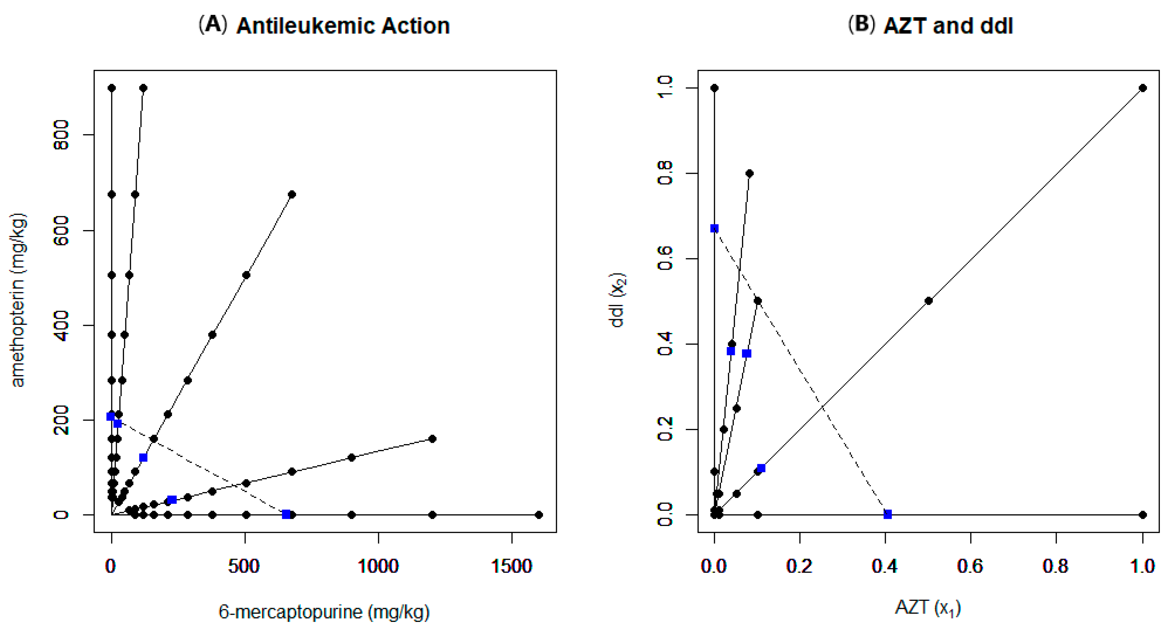
To investigate the interaction effect of anti-cancer agents 6-mercaptopurine and amethopterin on mortality in mice, Ref. [7] reports a study involving 464 mice randomized to various doses of these agents alone or in mixture in a 2 + 3 ray design. Thus, this dataset’s experimental design included the single-action rays plus three interior rays. The chosen amethopterin-to-6-mercaptopurine ratios (i.e., slopes) of the interior rays are 7.5:1 (slope c 3 = 7.5 ), 1:1 (slope c 4 = 1 ), and 1:7.5 (slope c 5 = 1 7.5 ), and includes 11–12 support points per ray with n = 8 mice per support point. The study involved 58 total support points and 464 mice. The 2 + 3 ray design and support points (filled circles) are plotted in Figure 3A. These data are well-fit by the binomial logistic model function with common slope parameter ( θ 3 ), π = d / θ 2 θ 3 1 + d / θ 2 θ 3 , where d representing the combined dose (i.e., the sum of 6-mercaptopurine and amethopterin) and with unique L D 50 parameters ( θ 2 ) for each of the five rays. The estimated L D 50 parameters are θ ^ 21 = 655.63 (ray 1), θ ^ 22 = 205.72 (ray 2), θ ^ 23 = 216.70 (ray 3), θ ^ 24 = 239.42 (ray 4), θ ^ 25 = 258.88 (ray 5). These estimated values are plotted in Figure 3A (filled squares), as is the estimated L D 50 line (dashed line) connecting θ ^ 21 = 655.63 on the horizontal axis with θ ^ 22 = 205.72 on the vertical axis. The estimated combination index values are κ ^ 3 = 0.97 (ray 3), κ ^ 4 = 0.76 (ray 4), and κ ^ 5 = 0.50 (ray 5) and the respective PLCIs are ( 0.73 ,   1.28 ) , ( 0.59 ,   0.99 ) , and ( 0.38 ,   0.64 ) . Examining these confidence intervals to see if they contain one (1), these data and this model suggests that independent action is detected along ray 3, marginal synergy is detected along ray 4, and strong synergy is detected along ray 5. Further, note that this fitted Separate Ray model did not exhibit lack of fit to the assumed model function.
Since the estimated L D 50 values do not line up as in the patterns shown in Examples 1–3, it is clear that the Finney model would provide a poor fit to these data. As such, the Separate Ray model is needed here since the assessment of whether interaction is declared here depends upon the respective mixtures (i.e., the ray slopes) of the anti-cancer agents.
Finally, as regards the chosen ray slopes, the equipotent slope ray here has slope c = θ ^ 22 θ ^ 21 1 3 here. Since the center ray here has slope c 4 = 1 and since from Equations (6) and (7), the estimated effective fractions are f ^ 3 = 0.04 ,   f ^ 4 = 0.24 , and f ^ 5 = 0.70 , the chosen design is spread more so towards the amethopterin (vertical) axis than the 6-mercaptopurine (horizontal) axis. Indeed, for these data, equi-spaced (uniform) values f ^ 3 = 0.25 ,   f ^ 4 = 0.50 , and f ^ 5 = 0.75 would correspond to instead using the slopes c 3 = 0.94 , c 4 = 0.31 , and c 5 = 0.10 . Further discussion of design strategies such as suggested ray slopes and number of support points per ray are given in Section 5.
The next illustration shows how the Separate Ray model can be adapted to response variable distributions other than the normal and binomial distributions assumed in the previous examples.

3.2. Example 5

In an in vitro study of the efficacy of the anti-HIV drugs AZT (zidovudine) and ddI (didanosine), Ref. [9] report data where the response variable is the amount of virus detected by reverse transcriptase (RT) activity (disintegrations per minute) units per 100 mL; for ease of analysis and presentation, the original AZT and ddI measurements have been scaled here by dividing by 10 and 1000, respectively. Figure 3B shows the plot of a portion of the chosen 2 + 3 ray experimental design with three interior rays. Plotted are 19 of the full design’s 24 support points (filled circles)—the highest level has been omitted from each ray in the plot to better facilitate more detailed viewing. This design includes replicate points taken at the origin (i.e., where both AZT and ddI are equal to zero). The rays of the interior rays here are c 3 = 10 , c 4 = 5 , and c 5 = 1 . Thus, the experimental design used in this study consisted of four doses of AZT alone, four doses of ddI alone, six combined doses in the 1:100 ratio, four combined doses in the 1:500 ratio and five combined doses in the 1:1000 ratio.
Since the response variable here is a count variable, popular candidate distributions are the Poisson and Negative Binomial (NB) distributions. The Poisson distribution leads to significant lack-of-fit here, but these data are well-fit by the NB distribution; see [71] for further discussions of lack of fit and overdispersion for these non-normal models. Furthermore, the mean model function here is E ( y ) = θ 1 1 + d / θ 2 θ 3 with a single common upper asymptote ( θ 1 ) and a single slope ( θ 3 ), but separate E C 50 parameters ( θ 2 r ) and combination index parameters ( κ r ) for each ray. Here, d is equal to the combined dose of AZT and ddI. Thus, along each ray, the assumed mean model function is this descending three-parameter dose response function starting from a height of θ 1 and descending to zero. The slope of decrease is measured by the parameter θ 3 , and for d = θ 2 r , the expected response is E ( y ) = θ 1 / 2 .
Parameter estimates for these data include θ ^ 21 = 0.41 (ray 1), θ ^ 22 = 0.67 (ray 2), θ ^ 23 = 0.42 (ray 3), θ ^ 24 = 0.45 (ray 4), θ ^ 25 = 0.22 (ray 5). These estimated values are plotted in Figure 3B using filled squares, as is the estimated E C 50 line (dashed line connecting θ ^ 21 = 0.41 and θ ^ 22 = 0.67 ). The estimated combination index values are κ ^ 3 = 0.67 (ray 3), κ ^ 4 = 0.75 (ray 4), and κ ^ 5 = 0.43 (ray 5) and the respective PLCIs are ( 0.47 ,   0.95 ) , ( 0.55 ,   1.06 ) , and ( 0.32 ,   0.58 ) . Examination of these confidence intervals to see if they contain one (1) leads to the conclusion that these data and this model find that independent action is detected along ray 4 but synergy is along rays 3 and 5. Interestingly, Ref. [9] assessed the interaction in these data using a rival model with a single interaction parameter assuming a normal distribution (with non-constant variance) and concluded that these data yield strong evidence of synergy. We prefer the Separate Ray model fit here since it allows for different modes of interaction along the different rays.
As was observed for the previous example; given the non-elliptical pattern in the estimated combination indices here; these data would be poorly fit using the Finney model and the richer Separate Ray model (along with NB distribution) is clearly needed.
The final illustration in this section highlights the need to sometimes extend the Separate Ray model to include unequal slopes along the rays.

3.3. Example 6

Data analyzed in [11] relate to the mortality of German cockroaches, Blattella germanica, to which petroleum distillate PD50 oil and/or 12 aliphatic alcohols was applied in Petri dishes. We consider here two of these alcohols, butanol and octanol, and their interaction with PD50 oil. Both studies involved 2 + 3 ray designs (i.e., with three interior rays) analogous to those examined and plotted in Figure 3. Along each ray, between 4 and 19 support points were chosen; at each point, the respective mixtures were applied to between n = 10 and n = 91 cockroaches. The slopes used in these studies were chosen so that the estimated effective fractions were approximately f ^ 3 = 0.20 ,   f ^ 4 = 0.50 , and f ^ 5 = 0.80 . Thus, since the L D 50 values (and thus relative potency) were well-estimated a   p r i o r i , the realized effective fractions were very close to the targeted 80:20, 50:50, and 20:80 mixtures.
In fitting these two datasets, it was required that the SR model be extended to allow for distinct slopes (in addition to distinct L D 50 values) along each ray. Then, these data were well-fit by the logistic model function, π = d / θ 2 r θ 3 r 1 + d / θ 2 r θ 3 r , where d is the combined dose (i.e., the sum of the PD50 oil amount and either the butanol or octanol amount). Notably, whereas these studies demonstrated that PD50 oil and butanol or octanol behaved synergistically along both ray 3 (80% butanol or 80% octanol versus 20% PD50 oil) and ray 4 (50:50 mixture), differing results were obtained for these alcohols for ray 5 (20% butanol or 20% octanol versus 80% PD50 oil). In the case of butanol, independent action was observed along ray 5, but for octanol, antagonism was indicated for this ray.
These results again clearly underscore the need for the SR model over the Finney model illustrated in Examples 1–3. That is, even though the Finney model was extended to allow for unequal slopes in Example 3, as shown in Figure 1, the Finney model requires that the combination indices line up in a certain manner and it cannot allow for synergy for one interior ray and antagonism for another.

4. Additional Applications and Extensions of Interaction Assessment

In this section, we provide further detailed extensions of the Finney and SR interaction models to illustrate the use of these methods with 96-well plates (or other blocking variables), when also modeling the variance function, when using horizontal cut-lines in place of the E C 50 line, and when studying/assessing three or more similar compounds. These topics are discussed in Examples 7–10.

4.1. Example 7

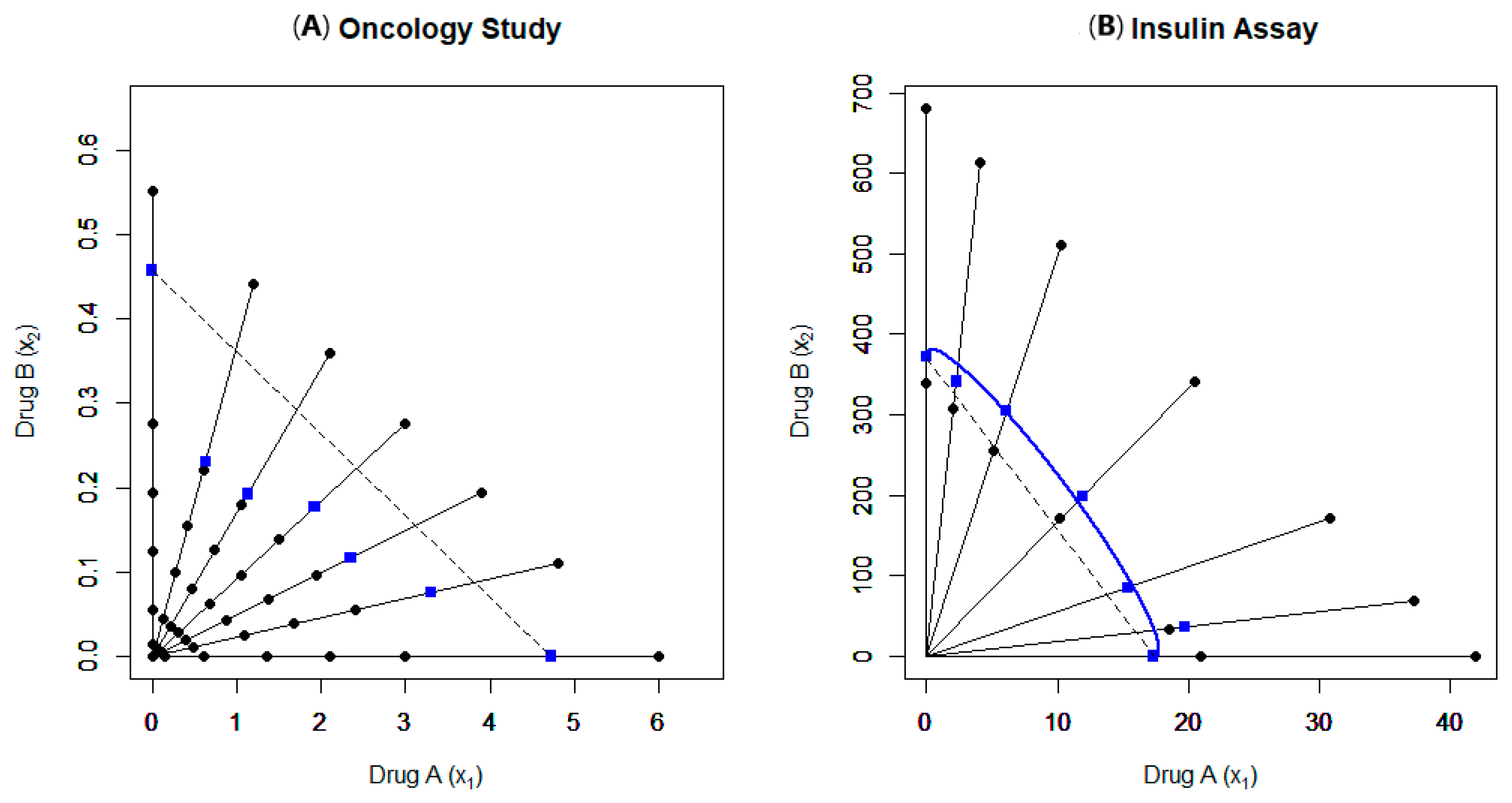
Data examined in [66] involve the interaction assessment of the effect of two oncology drug compounds on a radioactivity response (measured as counts per minute). The analysis here delves deeper into the full data than that used in [66] since, instead of the data subset used in [66], we use the full dataset and a richer model. This study involved nine 96-well plates so that each plate comprised a 2 + 5 ray design (i.e., with five interior rays corresponding to mixtures of compounds). Figure 4A shows a portion of the experimental design employed for only one of the plates in this study (plate 2) with the plotted support points (filled circles) (The complete dataset for this plate includes drug A concentrations up to 90 and drug B concentrations up to 8.28. These outer reaches of the plot were omitted only in this plot (but not in the analysis) so as to better visualize the estimated E C 50 values.). The experimental design used in the full dataset analyzed here included between 5 and 12 support points per ray (depending upon the plate).
One challenge here is how (statistically) to account for the plate effects, which are similar to block effects. After exploration, it was deemed best to assume a random effect term for plates in an analogous manner to the random effects used for chambers in Example 1. Furthermore, it is not uncommon that responses vary across the rows and/or columns of the 96-well plates, so we also included regression coefficients (up to second order) to adjust for any row and column effects. We also observed some aberrant values for runs in columns 5 and 9 of plate 3, and, instead of dropping these suspected outlier values, we included them in the analysis along with a dummy variable to adjust for their unusual response values. After adjusting for these effects, the (conditional) mean response is modeled here using the three parameter log-logistic model, E ( y ) = θ 1 1 + d / θ 2 θ 3 , where d = x 1 + x 2 is total dose. In this model function, θ 1 is the expected (adjusted) response at the origin, x 1 = x 2 = 0 (called the upper asymptote here since this model function is down-sloping from θ 1 to zero), θ 2 is the E C 50 parameter, and θ 3 is the slope of this dose–response function.
Since the response variable here is a count variable, it is in line with these data that the normal distribution be used (rather than the Poisson or Negative Binomial distribution) with the equal slope SR model fit and with the variance modeled by the function, v a r ( y ) = σ 2 E ( y ) ρ ; a useful discussion of the advantages of modeling variance instead of transforming one or both side of a linear or nonlinear model can be found in [44]. Note that when ρ = 0 , this variance function yields the homoscedastic value of σ 2 , whereas when ρ > 0 , the variance decreases with the mean, and this is a common phenomenon observed in several dose–response datasets.
For these data, the average (random) upper asymptote was estimated to be θ ^ 1 = 3855 and the estimated plate-to-plate variability of the upper asymptotes was σ ^ u = 460 . There was also detected a significant additional plate row effect ( p = 0.0002 ), and, by including plate rows in the model, the excess row variability is removed from the interaction assessment. Further, with the estimate ρ ^ = 1.33 (and CI of ( 1.20,1.46 ) ), these data exhibited non-constant variance decreasing with the mean. Additional parameter estimates here are θ ^ 21 = 4.72 (ray 1), θ ^ 22 = 0.46 (ray 2), θ ^ 23 = 0.86 (ray 3), θ ^ 24 = 1.32 (ray 4), θ ^ 25 = 2.10 (ray 5), θ ^ 26 = 2.47 (ray 6) and θ ^ 27 = 3.38 (ray 7). These estimated values are plotted in Figure 4A using filled squares, as well as the estimated E C 50 (dashed) line. The estimated combination index values here are κ ^ 3 = 0.64 (ray 3), κ ^ 4 = 0.66 (ray 4), κ ^ 5 = 0.80 (ray 5), κ ^ 6 = 0.75 (ray 6) and κ ^ 7 = 0.87 (ray 7), and tests of independent action ( H 0 : κ r = 1 ) were all rejected here with p-values less than or equal to p = 0.0027 , which is significant even after adjusting for multiple testing. Thus, these data suggest that these oncology drugs exhibit significant synergy. Perhaps because the richer dataset and a richer model is used here, our results indicate synergy along all interior rays whereas the analysis in [66] only detects synergy along certain rays.
We also underscore that the estimated effective fractions here are f ^ 3 = 0.21 ,   f ^ 4 = 0.36 , f ^ 5 = 0.51 , f ^ 6 = 0.66 and f ^ 7 = 0.81 . These values provide a near-uniform spread from approximately 0.2 to 0.8, and this underscores the superiority of the chosen slopes and design used here.

4.2. Example 8

Ref. [72] presents data related to a study of the interaction of standard insulin ( x 1 ) and A1-B29 suberoyl insulin ( x 2 ) where the response variable is the conversion of (3-3H) glucose to toluene-extractable lipids in rat fat cells ( y ). The chosen design is a 2 + 5 ray design (i.e., a ray design with five interior rays) and the design points (combinations of inputs) are plotted as the 14 filled circles in Figure 4B. Due to the nature of the response here and the fact that there are only two support points on each ray (i.e., preventing the fitting of a richer model function), the assumed distribution here is homoscedastic normal with dose response mean model function, E ( y ) = θ 1 z 3 θ 2 + z . In this expression, θ 1 is the upper asymptote (the expected response for z very large). Further, θ 2 is the E D 25 and is such that when z = θ 2 ,   E y = θ 1 4 . Note that we estimate E D 25 values here using the model function E ( y ) = θ 1 z 3 θ 2 + z instead of estimating E D 50 values using the model function E ( y ) = θ 1 z θ 2 + z for these data since there are only two support points per ray and since the plotted data show only the initial lower (upsloping) regions of the dose response curves. Thus, estimation of the E D 25 values is more stable than estimation of the E D 50 values here.
For the Finney version of this model function, z = x 1 + θ 4 x 2 + θ 5 θ 4 x 1 x 2 (see Equation (1)), and for the Separate Ray (SR) version of this model function, z = x 1 + x 2 (see Section 3). Note that in both cases, the E D 25 parameters here vary by ray: the Finney model requires that these E D 25 parameters values line up according to the elliptical relation illustrated and discussed in Section 2 and Section 3, but the SR model imposes no such constraint. For these data, when fitting both the Finney and the SR models, generalizing the above models to allow for different upper asymptotes ( θ 1 ) for the different rays was deemed an unnecessary generalization, so a common θ 1 is used here.
The Finney model fit parameter estimates for these data are θ ^ 1 = 50.41 ,   θ ^ 2 = 17.35 , θ ^ 4 = 0.047 and θ ^ 5 = 0.32 . Focusing on the interaction assessment, due to the negative coefficient of synergy estimate, θ ^ 5 = 0.32 , antagonism is tentatively retained. Further, the 95% PLCI for θ 5 is ( 0.54 , 0.074 ) ; since both endpoint of this interval are negative, this Finney model indicates that these two versions of insulin act antagonistically. The p-value for testing for independent action ( H : θ 5 = 0 ) is p = 0.0130 . The significant antagonism here can be seen in Figure 4B, where the bowing-outward 25% isobole (partial ellipse) is plotted. This plotted isobole connects θ ^ 2 = 17.35 on the horizontal axis with θ ^ 2 / θ ^ 4 = 371.38 on the vertical axis (the E D 25 line is the dashed line).
When the SR model is instead fitted to these data, one obtains for rays 3–7 the following estimated E D 25 values: θ ^ 23 = 343.61 , θ ^ 24 = 310.84 , θ ^ 25 = 210.87 , θ ^ 26 = 100.69 and θ ^ 27 = 56.24 . These values are plotted in Figure 4B using the filled squares. Note that these estimated E D 25 values very nearly follow the plotted Finney isobole (with only appreciable deviation for Ray 7). The corresponding combination index estimates are κ ^ 3 = 0.995 ,   κ ^ 4 = 1.14 ,   κ ^ 5 = 1.23 ,   κ ^ 6 = 1.16 , and κ ^ 7 = 1.30 . Of these, the only 95% PLCIs which exclude the value one (1) are those for rays five and seven. Further, so as to adjust for multiple testing, using a 99% instead of 95% confidence level, the only 99% PLCI which excludes the value one (1) is ray 7.
This latter SR analysis notwithstanding, the test here comparing the Finney and SR models indicates that the more parsimonious Finney model fits these data well, and antagonism is detected.
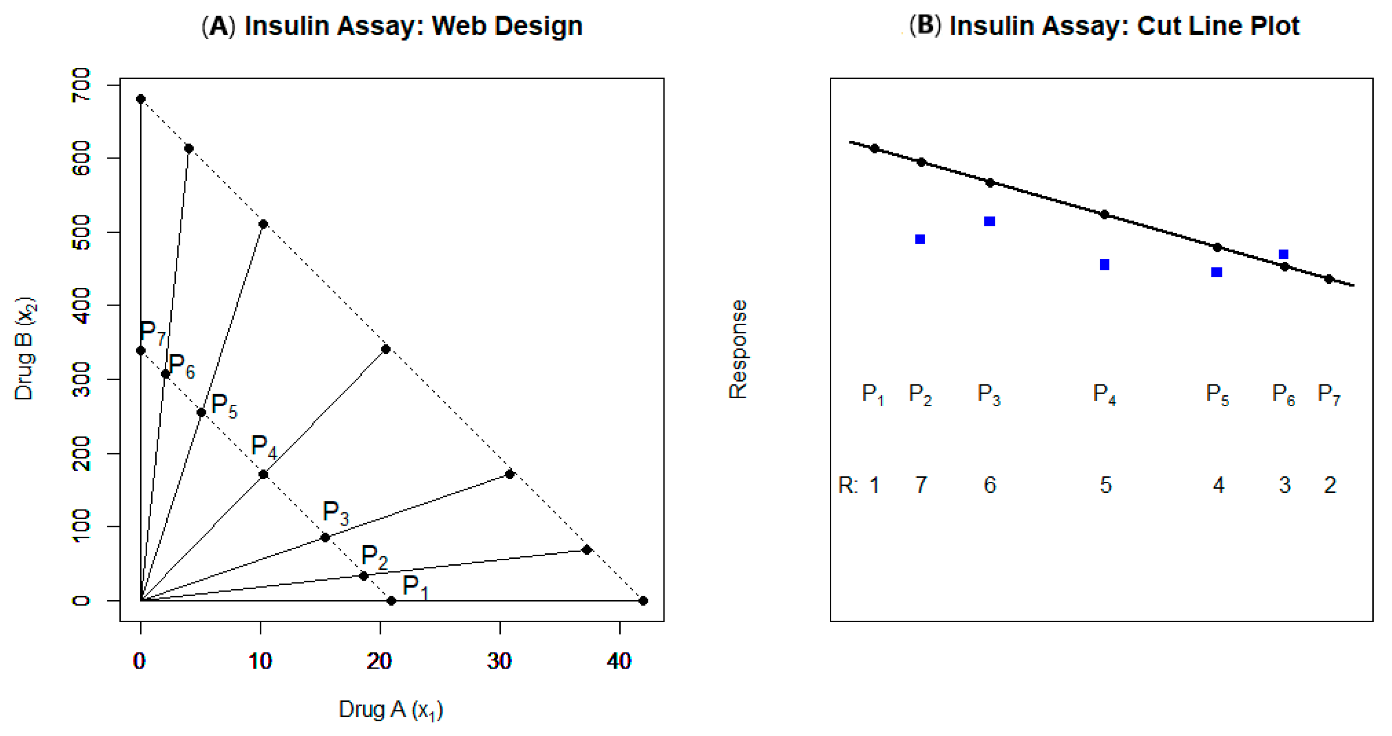
The experimental design used for this illustration are redrawn in Figure 5A; it allows us to develop a new technique for assessing synergy/antagonism and to delve deeper into these data’s interaction assessment. We call the chosen design here a ‘web design’ since all of the chosen design support lines occur at the intersection of rays and cut lines. The two chosen cut lines here are of the form
x 1 a k + x 2 b k = 1
Although Equation (9) resembles Equation (4), notice there is a crucial difference. In Equation (4), x 1 and x 2 are divided by the (unknown) E C 50 points θ 21 and θ 22 , whereas in Equation (9), they are divided by the fixed numbers a k and b k (i.e., not parameters to be estimated). Thus, for this study, a 1 = 20.9 and b 1 = 340 for the first cut line (i.e., the line closest to the origin) and a 2 = 41.9 and b 2 = 681 for the second cut line. Further, in Figure 5A, we have labeled the intersection points of the rays with the inner cut line by P 1 through P 7 and these points are redrawn Figure 5B (in reverse order) where the plotted row labeled “R” at the bottom of the plot corresponds to the ray number.
In what follows, we focus solely on this first cut line; comparable results could be derived for the second cut line. Next, we algebraically derive our cut line combination indices proceeding in two steps; note that some readers may wish to skip the algebraic details derived here and instead use Equation (11). The first challenge is to obtain a parametric equation of the solid line plotted in Figure 5B. Denote the values of the assumed response function for a 1 and b 1 by η a 1 = η ( a 1 , 0 ) and η b 1 = η ( 0 ,   b 1 ) respectively. Then, at any value ( x 1 , x 2 ) on this line with x 1 ( 0 , a 1 ) and x 2 = b 1 b 1 a 1 x 1 , the response is denoted η x 1 , x 2 = η d for combined dose d = x 1 + x 2 . Algebraic results then confirm that the line which connects the points ( a 1 , η a 1 ) with ( b 1 , η b 1 ) , estimated and plotted in Figure 5B is
y x 1 ,   x 2 = η a 1 + η b 1 η a 1 1 x 1 a 1
The next step is to derive the value of the combination index in the spirit of those derived in Section 3 for the Separate Ray model. For each of the interior rays of a web design, we define the ‘cut line combination index’ by dividing the actual functional height at the point ( x 1 , x 2 ) by the predicted or expected value from the line in Equation (10). To again make it be the case that combination index values less than one indicate synergy and greater than one indicate antagonism, we are forced to distinguish the two cases where the model response function is monotonically increasing and where it is monotonically decreasing (the only cases considered). In the increasing case (as is the case for this example), this first cut line and ray r (i.e., where x 2 = c r x 1 ), the cut line combination index is defined by
λ 1 r = y x 1 ,   x 2 η ( d ) = b 1 η a 1 + c r a 1 η b 1 b 1 + c r a 1   η ( d )
For the decreasing model function case, λ 1 r is simply defined to be the reciprocal, η ( d ) / y x 1 ,   x 2 , and again, this is so defined so that λ 1 r < 1 implies synergy and λ 1 r > 1 implies antagonism for both monotonically increasing and monotonically decreasing model functions. Understanding this cut line combination index in the increase case can be achieved by examining the middle expression in Equation (11), y x 1 ,   x 2 η ( d ) , which is the ratio of the fitted line value (akin to connecting equal potency points but using response values) to that predicted for this point using the actual data: if it is greater than one, then the actual data’s predicted point is not up to the response level expected under the no interaction (linear) condition.
To further illustrate this model fit using these data, the parameter estimates are λ ^ 13 = 0.99 ,   λ ^ 14 = 1.10 ,   λ ^ 15 = 1.16 ,   λ ^ 16 = 1.11 and λ ^ 17 = 1.21 (for the first cut line) and λ ^ 23 = 0.99 ,   λ ^ 24 = 1.08 ,   λ ^ 25 = 1.12 ,   λ ^ 26 = 1.08 and λ ^ 27 = 1.16 (for the second cut line). The first cut line’s estimated cut line combination indices can be visualized in Figure 5B where the estimated/fitted values η ( d ) are plotted above the respective rays (filled squares) and where the points on the solid line from Equation (1) are the indicated filled circles. Recall that the λ 1 r values are the value on the line divided by these fitted η ( d ) values so that λ 1 r > 1 (antagonism) means that the line exceeds the fitted value. To the extent that any estimated λ 1 r values significantly exceed one, then, this would be an indication that the actual model/data values are significantly lower than what is expected from the ‘equal potency counterpart’ line.
Assessing significance here depends upon the chosen level of significance. At the α = 0.05 level, significant antagonism is again detected (for both cut lines) along rays five (5) and seven (7). So as to again adjust for multiple testing, at the stricter α = 0.005 level, significant antagonism is again detected (for both cut lines) only along ray seven (7). This methodology provides more insight than the Finney analysis presented above but the results here exactly mirror those of the SR model. Although further extensive exploration and research are needed, the cut line combination index approach may be better than the SR model approach in situations where for dose response situations interaction may be detected for lower response values but not for higher values (or vice versa). This follows since the usual SR model examines behavior for, say, E C 50 or E C 25 values, whereas the cut line approach can be used for cuts at several expected heights such as at 20%, 40%, 60% and 80%. This illustration also underscores a major difference between the SR and the cut-line approach: whereas the SR model fit here includes five combination index (interaction) parameter, the cut-line approach doubles that number to ten cut-line combination indices as given in Equation (11) (but for both cut lines). Additional comments contrasting the Finney, SR and cut-line approaches are given in Section 5.
These data and this model indicate that antagonism is clearly detected along ray seven. It should be noted that since θ ^ 21 = 16.29 and θ ^ 22 = 399.0 , ray seven’s estimated effective fraction is f ^ = 0.93 , so that this ray leans very heavily toward standard insulin (plotted on the horizontal axis in Figure 4B) instead of A1-B29 suberoyl insulin (plotted on the vertical axis in the graph).
We next consider extensions to studying interaction of three (or more) similar compounds.

4.3. Example 9

In a controlled environmental toxicology study involving aquatic test chambers, Ref. [12] examines the effect of heavy metals (copper (CU), zinc (ZN) and nickel (NI)) on 4 day-old larval fathead minnows using a 96 h renewal acute toxicity test. The study involved 38 total support points of negative control, one-metal alone concentrations, and all three pairs of metals combinations. Although pairs of metals are considered here, note that no three-way combinations were examined in this study. The average number of minnow larvae per treatment combination (i.e., design support point) was approximately 40, so there were 1540 total minnow larvae used in this study. Since the response here is cumulative mortality over the 96 h period, a binomial distribution is assumed; diagnostic plots and analysis validated this assumption. We next extend the Finney model in Equation (2) to this three-compound situation by defining the effective concentration here as
z = C U + θ 42 Z N + θ 43 N I + θ 512 θ 42 × C U × Z N + θ 513 θ 43 × C U × N I + θ 523 θ 42 × θ 43 × Z N × N I
In this expression, θ 42 is the relative potency parameter representing the conversion of Z N to C U and θ 43 is the relative potency parameter converting N I to C U . Moreover, θ 512 ,   θ 513 , and θ 523 are the three coefficients of synergy terms used to assess the three pairwise (two-at-a-time) interactions. Since mortality here decreases with metal concentration, to relate the effective concentration in Equation (12) to percent mortality, we assessed the rival models π = 1 1 + z / θ 2 θ 3 and π = 1 1 + e θ 3 z θ 2 , where in both cases θ 2 is the E C 50 parameter and θ 3 is the slope parameter. Here, it was found that the latter model fit these data better. This underscores the importance of using the proper (indicated) scale in nonlinear modeling. The first model given here (called the LL2 model) uses the log-concentration scale and the second model (called the LOG2 model) uses the un-transformed concentration scale. As demonstrated in [73] these two models are special cases of a larger model, the Scaled Logistic model, which can thereby facilitate statistical testing. Note that attempts to fit a richer model such as an extension of the SR model would not fit for these data since, although the study was designed as involving three interior rays (with one interior ray on each pairwise combination plane), the actual applied concentrations used deviated appreciably from the given rays. This can occur in practice if the intended doses or concentrations differ from those actually received by the experimental units and so the latter points deviate from the rays.
For this three-compound pairwise Finney model (using the LOG2 scale), the parameter estimates are θ ^ 2 = 128.84 (the estimated E C 50 for C U ), θ ^ 3 = 0.034 , θ ^ 42 = 0.14 (so the estimated E C 50 for Z N is θ ^ 22 = 128.84 / 0.14 = 916.11 ), θ ^ 43 = 0.033 (so the estimated E C 50 for N I is θ ^ 23 = 128.84 / 0.033 = 3931 ), θ ^ 512 = 0.98 ,     θ ^ 513 = 2.97 , and θ ^ 523 = 1.26 . Notably, the 95% PLCIs for these three coefficients of synergy (the θ 512 ,   θ 513 and θ 523 terms) are ( 0.48 ,   1.54 ) , ( 2.25 ,   3.79 ) , and ( 0.80 ,   1.78 ) , respectively.
As for the two-compound Finney model, these coefficient of synergy confidence intervals are examined to see if they contain zero (0). Since they all lie above zero, synergy is declared here between C U and Z N , between C U and N I , and between Z N and N I . One caveat, however, is that had the experimental design used here included runs with all three metals applied, we would then have been able to then check for three-way interaction.
Along the lines of the above caveat, the next illustration allows for the assessment of this three-way interaction since it uses the indicated richer experimental design.

4.4. Example 10

Data reported in [74] are from a study of 400 Chinese female patients who underwent elective gynecological surgery and who were randomized to between one and three of the sedative drugs midazolam (‘ m ’), propofol (‘ p ’), and alfentanil (‘ a ’). The chosen experimental ray design included the three single-drug rays, one interior ray for each of the drug pairs and one interior ray for the triple combination (i.e., 3 + 3 + 1 = 7 total rays) with 5–8 support points per ray, 40 total support points, and n = 10 women randomized per support point (i.e., drug combination). The outcome variable of the data analyzed here ( y ) is whether the woman was hypnotized (i.e., failure to open their eyes upon verbal command). This response variable was assumed to follow the binomial distribution for the given n = 10 women for each design support point. For these data, the logistic model fits slightly better on the LOG scale, so that we model π = e θ 3 d θ 2 1 + e θ 3 d θ 2 , where θ 2 and θ 3 are the respective L D 50 and slope parameters, d = z for the Finney model.
The Finney model in Equation (12) is easily extended here to include the three-way interaction term by defining the effective concentration in this situation as
z = m + θ 42 p + θ 43 a + θ 512 θ 42 m p + θ 513 θ 43 m a + θ 523 θ 42 θ 43 p a + θ 5123 θ 42 θ 43 m p a 3
Note especially that the 1 / 3 power on the triple combination in this expression preserves the measured unit scale since three terms are multiplied for this term. In the equal-slope case, the parameter estimates are θ ^ 2 = 0.15 ,     θ ^ 3 = 35.6 ,     θ ^ 42 = 0.15 ,     θ ^ 43 = 1.59 ,     θ ^ 512 = 1.04 ,     θ ^ 513 = 1.49 ,     θ ^ 523 = 0.35 , and θ ^ 5123 = 1.00 . The negative sign attached to the last parameter estimate suggests that when combined, these three drugs interact in an antagonistic manner. That said, the associated 95% PLCI for θ 5123 , ( 2.07 ,   0.03 ) , actually includes zero—although just barely so. Thus, to the extent that this equal-slope Finney model (using the LOG scale) fits these data, we cannot reject the claim of three-way independent action. We next explore the Separate Ray (SR) model here in an attempt to increase the estimation precision.
To extend the SR model introduced and illustrated in Section 3 to this three-drug situation, let p = c 4 m ,   a = c 5 m , and a = c 6 p denote the rays 4–6 in the p m , a m , and a p planes, respectively. Also, let both p = c 71 m and a = c 72 m together denote ray 7 in the combined three-dimensional space. Defining combination indices is as follows (with κ 4 for ray 4 in the p m plane, κ 5 for ray 5 in the a m plane, κ 6 for ray 6 in the a p plane, and κ 7 for ray 7 in the p m a three-dimensional space), algebraic manipulation can be used to show that
κ 4 = m θ 21 + p θ 22 = θ 24 θ 22 + c 4 θ 21 1 + c 4 θ 21 θ 22 ,       κ 5 = m θ 21 + a θ 23 = θ 25 θ 23 + c 5 θ 21 1 + c 5 θ 21 θ 23 , κ 6 = p θ 22 + a θ 23 = θ 26 θ 23 + c 6 θ 22 1 + c 6 θ 22 θ 23 ,     κ 7 = m θ 21 + p θ 22 + a θ 23 = θ 27 θ 22 θ 23 + c 71 θ 21 θ 23 + c 72 θ 21 θ 22 1 + c 71 + c 72 θ 21 θ 22 θ 23
Next, using d = combined dose and unequal slopes ( θ 3 ) along the rays, the estimated combination indices here are κ ^ 4 = 0.64 ,   κ ^ 5 = 0.53 ,   κ ^ 6 = 0.82 , and κ ^ 7 = 0.59 . Although each of κ ^ 4 ,   κ ^ 5 and κ ^ 6 are significantly less than one (implying pairwise synergy), the fact that κ ^ 7 > κ ^ 5 indicates possible three-way antagonism, which then agrees with the marginal Finney model results above. Next, one measure which can be proposed to assess three-way interaction for this SR model—using a ratio and product here in the spirit of [75,76]—is
ρ = κ 7 κ 4 κ 5 κ 6
Evidence of synergy is declared here when ρ < 1 and evidence of antagonism occurs for ρ > 1 . Here, ρ ^ = 2.15 , and the test H 0 : ρ = 1 is rejected ( χ 1 2 = 5.59 ,   p = 0.0180 ), thereby indicating three-way antagonism. Along the same lines, it is interesting and noteworthy to point out that when the Finney model above is fit on the log-dose scale (i.e., the LL2 format), the 95% PLCI for θ 5123 , ( 2.25 ,   0.05 ) , does (barely) exclude zero.
In sum, the overall conclusion here is that these data suggest there is marginal evidence of three-way antagonism between midazolam, propofol, and alfentanil in their effect on patient hypnosis. Clearly, these data and results indicate that a larger study is needed of these three compounds.

5. Discussion

Assessing interaction is paramount in applied research. When asked which treatment is best, an answer such as ‘it depends’ often means some kind of interaction may be present, and it needs to be explored and understood. As noted in Section 1, classical two-way ANOVA assessment of interaction and linear methods such as response surface techniques can often be found to be inadequate, and as such, our focus here has been on nonlinear interaction assessment. The appropriate interaction measure one chooses to use generally depends upon where in the research process one is, and nonlinear assessment is often used as researchers become more familiar with the quantitative behavior of the factors under study. The measures we have introduced and illustrated here include the Finney model (and variations), the Separate Ray model (which can be easily extended to horizontal, vertical, checkerboard, and factorial designs in addition to the ray designs used here), web designs with cut lines methods, and extensions to three or more compounds. The level of sophistication of the model used by a practitioner clearly depends upon the goals of the study, the example details, the experimental design used, and prior experiences in the research process. The focus in this concluding section is on providing concise advice to the practitioner interested in interaction assessment—including comparing and contrasting the Finney, SR and cut-line approaches—and using the chosen examples to provide important take-home messages.
The ten illustrations discussed here are summarized in Table 1. This table underscores that the provided illustrations generally increase in complexity with the example number: this in turn often necessitates the use of a more intricate model. The nature of the response variable indicates the choice of the assumed distribution, and the chosen distributions used here ranged from the normal to binomial to Poisson and negative binomial (NB). As in the examples, we usually first fit the appropriate Finney model and check for lack of fit. Examples 4–6 highlight a potential shortcoming of the Finney model in that it employs a single interaction parameter and so it may not be appropriate in assessing interaction for certain datasets. Example 9 also underscores that the appropriate scale used in the model function needs to be considered. Many of the illustrations used ray designs but some (e.g., Example 9) found this impractical; fortunately, as noted above, the Separate Ray (SR) model can be fit even to non-ray-design data such as factorial designs. As such, fitting the SR model may highlight any inadequacies of the Finney model. Should the chosen experimental design be a web design (i.e., with cut lines), the cut-line combination index modeling approach used in Example 8 may provide an even-richer and better fit to the data than the SR model. Finally, the indicated study limitations in Table 1’s ‘Notes’ column serve as an aid to the researcher in choosing the experimental design, and design issues are discussed further below. In sum, we advocate choosing a simpler model which adequately summarizes the interaction study and data, proceeding to a more complex model only as needed (e.g., notable lack of fit of the simpler model).
As underscored in Table 1 and [77,78,79,80,81,82,83], the chosen experimental design can be essential for interaction assessment. We generally advocate the use of a ray design (if not a web-design) with three interior rays (and perhaps 3–4 cut line). But clearly this one-size-fits-all approach should be adapted for the goals and constraints of a given specific study. Table 1 highlights that in binomial situations, choosing too many design support points per ray can result in values of n (i.e., samples per design point) which are quite small (e.g., only n = 8 in Example 4 and n = 10 in Example 10). A better approach is observed in Example 2, which used a 2 + 3 ray design (i.e., with 3 interior rays) with (approximately) n = 30 and four support points per ray. The chosen design in Example 2 also employed geometric spacing of the design points along the rays; studies such as [73,82,83] show that these geometric designs are commonplace and can often be quite efficient in practice. Similar comments apply in non-binomial cases too, where n is the number of replicates per support point, and larger n generally results in higher precision and smaller experimental error. Optimal design strategies as discussed in [77,80] may be considered, but, as discussed in [81,82,83], we generally tend to prefer near-optimal designs which also provide information to detect lack-of-fit. Note also that the D-optimal design for the Finney model comprises six support points (two points on each of the horizontal and vertical axes and on a single ray of slope 1 / ρ ), with the two support points on either side of the respective E C 50 points. Research along these lines for nonlinear interaction studies is currently ongoing.
Several of the illustrations in Table 1 underscore the fact that before a ray design can be chosen, in order to get a good spread of the rays (e.g., f = 0.25 ,   0.50 and 0.75 in Equation (6)), researchers first need accurate information about the relative potency ( ρ ) of the compounds under study. To see this, note that re-writing Equation (7) gives c = 1 f f ρ . Thus, the equally spaced ray choices f = 0.25 ,   0.50 and 0.75 coincide with respective slopes c = 3 ρ ,   1 ρ and 1 / 3 ρ . This dependence demonstrates the need to first possess an accurate estimate of the relative potency ( ρ ); as noted above, having such an accurate estimate is also required before a D-optimal design can be chosen for the Finney model. Thus, as advocated in [66], if practical, it may be wise to first run a preliminary study to estimate the relative potency of the compounds before proceeding to designing and assessing the full interaction study.
Employing a reasonably estimated relative potency, a ray design with 2–3 interior rays (with or without cut lines) can then be designed perhaps with 4–5 geometric support points per ray. Interaction assessment modeling would entail fitting the Finney model, with the SR and-or cut-line models fit and used as needed should the Finney model prove inadequate. The key model parameter estimate(s) are then used to summarize and assess any interactions.
The three interaction models considered here—the Finney, the Separate Ray (SR) and the cut-line combination index (CLCI) approaches—are summarized and compared in Table 2 which provides important pros and cons of these models. As noted above, it is generally advised to start with the simpler (Finney) model and proceed to more complex model(s) as needed—e.g., should the Finney model exhibit lack-of-fit. Although it is a somewhat simple model, the Finney model may be preferred as it straightforward to fit and includes only a single interaction summary measure (and model-fitting algorithms will usually converge). That said, several of the practical datasets given in Table 1 required (at least) the SR model since interaction is not well-summarized for these illustration datasets with a single interaction measure. Fitting a more complex model such as the SR or CLCI model generally involves a more complex design, with rays and possibly with cut-lines. Research results (via simulations) involving specific instances and conditions where the SR and CLCI models are contrasted is ongoing and outside the scope of the current work, but it is readily apparent that the CLCI model will provide a better fit than the SR model if the interaction assessment varies when the behavior varies at a (response) height of, for example, 25% versus at a height of 75%. Another important topic of ongoing research is to extend the results given here to focus on the therapeutic window enhancement between (drug) efficacy and toxicity discussed in [23].
Finally, as noted in Table 2, fitting the CLCI model to a web design with ( R 2 ) interior rays and C cut lines results in C ( R 2 ) interaction parameters, and concerns of overfitting and multiple comparison adjustment of the type I error rate needs to be taken into account. To illustrate, in the aforementioned illustration of three interior rays and four cut lines, there would be 12 cut-line combination index (interaction) parameters, and, along the lines of Scheffe’s adjustment for testing all contrasts (see [84]), it may then be wise to use say α = 0.005 (instead of the usual α = 0.05 ) as the type I error rate to avoid overfitting the given data. As noted, research into these issues so as to provide practical rules of thumb as well as robust design strategies is ongoing.

Funding

This research benefited from a Fulbright scholarship grant from the Fulbright Scholar Program, which is gratefully acknowledged for supporting the author’s visit to the Budapest University of Technology and Economics.

Institutional Review Board Statement

Not applicable.

Informed Consent Statement

Not applicable.

Data Availability Statement

Subject to needed permission and approval, SAS® and/or R computer code and data used in this article made available upon email request.

Acknowledgments

The insightful and comprehensive comments and suggestions of three anonymous reviewers are gratefully acknowledged; these comments have resulted in significant improvements to initial drafts of this paper. The author also expresses his gratitude for thoughtful discussion with, suggestions and comments from his Budapest University of Technology and Economics Applied Statistics post-graduate students as well as his Loyola University Chicago Advanced Biostatistics undergraduate and Master’s students.

Conflicts of Interest

No form of artificial intelligence or software (such as ChatGPT) was used in the preparation or revision of this work. The author declares no conflicts of interest.

Abbreviations

The following abbreviations are used in this manuscript:
CIConfidence interval
LALower asymptote
LSELeast-squares estimate
MLEMaximum likelihood estimate
MSEMean squares estimate (of variance)
NESNot-equal slope (model)
PLCIProfile likelihood confidence interval
REMLRestricted maximum likelihood (estimate)
SR(M)Separate ray (model)
UAUpper asymptote

References

  1. Heggestad, H.E.; Bennett, J.H. Photochemical Oxidants Potentiate Yield Losses in Snap Beans Attributable to Sulfur Dioxide. Science 1981, 213, 1008–1010. [Google Scholar] [CrossRef] [PubMed]
  2. Heagle, A.S.; Heck, W.W.; Rawlings, J.O.; Philbeck, R.B. Effects of Chronic Doses of Ozone and Sulfur Dioxide on Injury and Yield of Soybeans in Open-Top Field Chambers. Crop Sci. 1983, 23, 1184–1191. [Google Scholar] [CrossRef]
  3. Hay, M.E.; Kappel, Q.E.; Fenical, W. Synergisms in Plant Defenses Against Herbivores: Interactions of Chemistry, Calcification, and Plant Quality. Ecology 1994, 75, 1714–1726. [Google Scholar] [CrossRef]
  4. Mauderly, J.L.; Samet, J.M. Is There Evidence for Synergy Among Air Pollutants in Causing Health Effects? Environ. Health Perspect. 2009, 117, 1–6. [Google Scholar] [CrossRef]
  5. Box, G.E.P.; Draper, N.R. Response Surfaces, Mixtures, and Ridge Analysis, 2nd ed.; Wiley: Hoboken, NJ, USA, 2007. [Google Scholar]
  6. Myers, R.H.; Montgomery, D.C.; Anderson-Cook, C.M. Response Surface Methodology: Process and Product Optimization Using Designed Experiments, 4th ed.; Wiley: Hoboken, NJ, USA, 2016. [Google Scholar]
  7. Goldin, A.; Venditti, J.M.; Humphreys, S.R.; Dennis, D.; Mantel, N.; Greenhouse, S.W. An Investigation into the Synergistic Antileukemic Action of Amethopterin and 6-Mercaptopurine in Mice. J. Natl. Cancer Inst. 1955, 16, 129–138. [Google Scholar]
  8. Gerig, T.M.; Blum, U.; Meier, K. Statistical Analysis of the Joint Inhibitory Action of Similar Compounds. J. Chem. Ecol. 1989, 15, 2403–2412. [Google Scholar] [CrossRef] [PubMed]
  9. Machado, S.G.; Robinson, G.A. A Direct, General Approach Based on Isobolograms for Assessing the Joint Action of Drugs in Pre-Clinical Experiments. Stat. Med. 1994, 13, 2289–2309. [Google Scholar] [CrossRef]
  10. Govindarajulu, Z. Statistical Techniques in Bioassay, 2nd ed.; Karger: Basel, Switzerland, 2001. [Google Scholar]
  11. Sims, S.R.; O’Brien, T.E. Mineral Oil and Aliphatic Alcohols: Toxicity and Analysis of Synergistic Effects on German Cockroaches (Dictyoptera: Blattellidac). J. Econ. Entomol. 2011, 104, 1680–1686. [Google Scholar] [CrossRef]
  12. Lynch, N.; Hoang, T.; O’Brien, T.E. Acute Toxicity of Binary-Metal Mixtures of Copper, Zinc, and Nickel to Pimephales Promelas: Evidence of More-Than-Additive Effect. Environ. Toxicol. Chem. 2015, 5, 446–457. [Google Scholar] [CrossRef] [PubMed]
  13. Son, J.; Lee, Y.-S.; Kim, Y.; Shin, K.-I.; Hyun, S.; Cho, K. Joint Toxic Action of Binary Metal Mixtures of Copper, Manganese and Nickel to Paronychiurus kimi (Collembola). Ecotoxicol. Environ. Saf. 2016, 132, 164–169. [Google Scholar] [CrossRef]
  14. Zimmermann, S.; Wolff, C.; Sures, B. Toxicity of Platinum, Palladium and Rhodium to Daphnia magna in Single and Binary Metal Exposure Experiments. Environ. Pollut. 2017, 224, 368–376. [Google Scholar] [CrossRef]
  15. Blum, U. Simple Phenolic Acids in Solution Culture I: pH and pKa. In Plant-Plant Allelopathic Interactions III; Blum, U., Ed.; Springer Nature Switzerland AG: Cham, Switzerland, 2019; pp. 71–113. [Google Scholar]
  16. Kumar, N.; Goel, N. Phenolic Acids: Natural Versatile Molecules with Promising Therapeutic Applications. Biotech. Rep. 2019, 24, e00370. [Google Scholar] [CrossRef] [PubMed]
  17. Makariadou, E.; Wang, X.; Hein, N.; Deresa, N.W.; Mutambanengwe, K.; Verbist, B.; Thas, O. Synergy Detection: A Practical Guide to Statistical Assessment of Potential Drug Combinations. Pharm. Stat. 2024, 24, e2383. [Google Scholar] [CrossRef]
  18. Muriel, J.; Escorial, M.; Carratalá, C.; Margarit, C.; Barrachina, J.; López, A.; Gallardo, E.; Kringen, M.K.; Peiró, A.M. Use of CYP2D6 Substrates and Inhibitors During Pain Management with Analgesic Opioids: Drug-Drug Interactions That Lead to Lack of Analgesic Effectiveness. Biomed. Pharmacother. 2024, 176, 116882. [Google Scholar] [CrossRef]
  19. Atkinson, A.C.; Donev, A.N.; Tobias, R.D. Optimum Experimental Designs, with SAS; Oxford University Press: Oxford, UK, 2007. [Google Scholar]
  20. Dai, N.; Ye, R.; He, Q.; Guo, P.; Chen, H.; Zhang, Q. Capsaicin and Sorafenib Combination Treatment Exerts Synergist Anti-hepatocellular Carcinoma Activity by Suppressing EGFR and PI3K/Akt/mTOR Signaling. Oncol. Rep. 2018, 40, 3235–3248. [Google Scholar] [CrossRef] [PubMed]
  21. Pal, M.; Mandal, N.K. Optimum Mixture Designs for the Log-logistic Dose-response Model with Mixture of Two Similar Compounds. Commun. Stat. Simul. Comput. 2018, 47, 800–808. [Google Scholar] [CrossRef]
  22. Pires, A.S.; Marques, C.R.; Encamação, J.C.; Abrantes, A.M.; Marques, I.A.; Laranjo, M.; Olivera, R.; Casalta-Lopes, J.E.; Gonçalves, A.C.; Sarmento-Ribeiro, A.B.; et al. Ascorbic Acid Chemosensitizes Colorectal Cancer Cells and Synergistically Inhibits Tumor Growth. Front. Physiol. 2018, 9, 911. [Google Scholar] [CrossRef]
  23. Weinstein, Z.B.; Kuru, N.; Kiriakov, S.; Palmer, A.C.; Khalil, A.S.; Clemons, P.A.; Zaman, M.H.; Roth, F.P.; Cokoi, M. Modeling the Impact of Drug Interactions on Therapeutic Selectivity. Nat. Commun. 2018, 9, 3452. [Google Scholar] [CrossRef] [PubMed]
  24. Amzallag, A.; Ramaswamy, S.; Benes, C.H. Statistical Assessment and Visualization of Synergies for Large-scale Sparse Drug Combination Datasets. BMC Bioinform. 2019, 20, 83. [Google Scholar] [CrossRef]
  25. Baek, I.-H.; Kim, Y.; Baik, S.; Kim, J. Investigation of the Synergistic Toxicity of Binary Mixtures of Pesticides and Pharmaceuticals on Aliivibrio fischeri in Major River Basins in South Korea. Int. J. Environ. Res. Public Health 2019, 16, 208. [Google Scholar] [CrossRef]
  26. Blangiardo, M.; Pirani, M.; Kanapka, L.; Hansell, A.; Fuller, G. A Hierarchical Modelling Approach to Assess Multi Pollutant Effects in Time-series Studies. PLoS ONE 2019, 14, e0212565. [Google Scholar] [CrossRef]
  27. Demidenko, E.; Miller, T.W. Statistical Determination of Synergy Based on Bliss Definition of Drugs Independence. PLoS ONE 2019, 14, e0224137. [Google Scholar] [CrossRef]
  28. Regan-Fendt, K.E.; Xu, J.; DiVincenzo, M.; Duggan, M.C.; Shakya, R.; Na, R.; Carson, W.E.; Payne, P.R.O.; Li, F. Synergy from Gene Expression and Network Mining (SynGeNet) Method Predicts Synergistic Drug Combinations for Diverse Melanoma Genomic Subtypes. NPJ Syst. Biol. Appl. 2019, 5, 6. [Google Scholar] [CrossRef] [PubMed]
  29. Robichaud, A.; Comtois, P. Environmental Factors and Asthma Hospitalization in Montreal, Canada, During Spring 2006–2008: A Synergy Perspective. Air Qual. Atmos. Health 2019, 12, 1495–1509. [Google Scholar] [CrossRef]
  30. Sidorov, P.; Naulaerts, S.; Ariey-Bonnet, J.; Pasquier, E.; Ballester, P.J. Predicting Synergism of Cancer Drug Combinations Using NCI-ALMANAC Data. Front. Chem. 2019, 7, 509. [Google Scholar] [CrossRef]
  31. Xiao, Q.; Wang, L.; Xu, H. Application of Kriging Models for a Drug Combination Experiment on Lung Cancer. Stat. Med. 2019, 38, 236–246. [Google Scholar] [CrossRef] [PubMed]
  32. Zhang, C.; Yan, G. Synergistic Drug Combinations Prediction by Integrating Pharmacological Data. Synth. Syst. Biotechnol. 2019, 4, 67–72. [Google Scholar] [CrossRef] [PubMed]
  33. Antonelli, J.; Mazumdar, M.; Bellinger, D.; Christiani, D.; Wright, R.; Coull, B. Estimating the Health Effects of Environmental Mixtures Using Bayesian Semiparametric Regression and Sparsity Inducing Priors. Ann. Appl. Stat. 2020, 14, 257–275. [Google Scholar] [CrossRef]
  34. Bagheri, O.; Moeltner, K.; Yang, W. Respiratory Illness, Hospital Visits, and Health Costs: Is it Air Pollution or Pollen? Environ. Res. 2020, 187, 109572. [Google Scholar] [CrossRef]
  35. Liu, H.; Zhang, W.; Zou, B.; Wang, J.; Deng, Y.; Deng, L. DrugCombDB: A Comprehensive Database of Drug Combinations Toward the Discovery of Combinatorial Therapy. Nucleic Acids Res. 2020, 48, D871–D881. [Google Scholar] [CrossRef]
  36. Nair, S.K.; Eeles, C.; Ho, C.; Beri, G.; Yoo, E.; Tkachuk, D.; Tang, A.; Nijrabi, P.; Smirnov, P.; Seo, H.; et al. ToxicoDB: An Integrated Database to Mine and Visualize Large-Scale Toxicogenomic Datasets. Nucleic Acids Res. 2020, 48, W455–W462. [Google Scholar] [CrossRef]
  37. Wambaugh, M.A.; Denham, S.T.; Ayala, M.; Brammer, B.; Stonhill, M.A.; Brown, J.C.S. Synergistic and Antagonistic Drug Interactions in the Treatment of Systemic Fungal Infections. eLife 2020, 9, e54160. [Google Scholar] [CrossRef]
  38. Yang, M.; Jaaks, P.; Dry, J.; Garnett, M.; Menden, M.P.; Saez-Rodriguez, J. Stratification and Prediction of Drug Synergy Based on Target Functional Similarity. NPJ Syst. Biol. Appl. 2020, 6, 16. [Google Scholar] [CrossRef] [PubMed]
  39. Wooten, D.J.; Meyer, C.T.; Lubbock, A.L.R.; Quaranta, V.; Lopez, C.F. MuSyC is a Consensus Framework that Unifies Multi-Drug Synergy Metrics for Combinatorial Drug Discovery. Nat. Commun. 2021, 12, 4607. [Google Scholar] [CrossRef]
  40. Zeuner, S.; Vollmer, J.; Sigaud, R.; Oppermann, S.; Peterziel, H.; ElHarouni, D.; Oehme, I.; Witt, O.; Milde, T.; Ecker, J. Combination Drug Screen Identifies Synergistic Drug Interaction of BCL-XL and Class I Histone Deacetylase Inhibitors in MYC-Amplified Medulloblastoma Cells. J. Neuro. Oncol. 2024, 166, 99–112. [Google Scholar] [CrossRef]
  41. Finney, D.J. Probit Analysis; Cambridge University Press: London, UK, 1971. [Google Scholar]
  42. Finney, D.J. Statistical Method in Biological Assay; Charles Griffin & Co.: London, UK, 1978. [Google Scholar]
  43. Ratkowsky, D.A. Nonlinear Regression Modeling: A Unified Practical Approach; Marcel Dekker: New York, NY, USA, 1983. [Google Scholar]
  44. Seber, G.A.F.; Wild, C.J. Nonlinear Regression; Wiley: New York, NY, USA, 1989. [Google Scholar]
  45. Ratkowsky, D.A. Handbook of Nonlinear Regression Models; Marcel Dekker: New York, NY, USA, 1990. [Google Scholar]
  46. Bates, D.M.; Watts, D.G. Nonlinear Regression Analysis and Its Applications; Wiley: New York, NY, USA, 2007. [Google Scholar]
  47. Archontoulis, S.V.; Miguez, F.E. Nonlinear Regression Models and Applications in Agricultural Research. Agron. J. 2015, 107, 786–798. [Google Scholar] [CrossRef]
  48. Jarantow, S.W.; Pisors, E.D.; Chiu, M.L. Introduction to the Use of Linear and Nonlinear Regression Analysis in Quantitative Biological Assays. Curr. Protoc. 2023, 3, e801. [Google Scholar] [CrossRef]
  49. O’Brien, T.E.; Silcox, J. Nonlinear Modelling: A Primer, Illustrations and Caveats. Bull. Math. Biol. 2024, 86, 40. [Google Scholar] [CrossRef]
  50. Hubert, J.J. Bioassay; Kendall/Hunt Publishing: Dubuque, IA, USA, 1980. [Google Scholar]
  51. Brunden, M.N.; Vidmar, T.J.; McKean, J.W. Drug Interaction and Lethality Analysis; CRC Press: Boca Raton, FL, USA, 1988. [Google Scholar]
  52. Berenbaum, M.C. What is Synergy? Pharmacol. Rev. 1989, 41, 93–141. [Google Scholar] [CrossRef]
  53. Barton, C.N.; Braunberg, R.C.; Friedman, L. Nonlinear Statistical Models for the Joint Action of Toxins. Biometrics 1993, 49, 95–105. [Google Scholar] [CrossRef]
  54. Gouws, E. Drug Resistance in Malaria Research—The Statistical Approach; Univ. Natal Pietermaritzburg Press: Scottsville, Africa, 1995. [Google Scholar]
  55. Greco, W.R.; Bravo, G.; Parsons, J.C. The Search for Synergy: A Critical Review from a Response Surface Perspective. Pharmacol. Rev. 1995, 47, 331–385. [Google Scholar] [CrossRef]
  56. Dawson, K.S.; Carter, W.H., Jr.; Gennings, C. A Statistical Test for Detecting and Characterizing Departures from Additivity in Drug/Chemical Combinations. J. Agric. Biol. Environ. Stat. 2000, 5, 342–359. [Google Scholar] [CrossRef]
  57. Tallarida, R.J. Drug Synergism and Dose-Effect Data Analysis; Chapman & Hall/CRC Press: Boca Raton, FL, USA, 2000. [Google Scholar]
  58. Bliss, C.I. The Toxicity of Poisons Applied Jointly. Ann. Appl. Biol. 1939, 26, 585–615. [Google Scholar] [CrossRef]
  59. Loewe, S. The Problem of Synergism and Antagonism of Combined Drugs. Arzneimittelforschung 1953, 3, 285–290. [Google Scholar]
  60. Fraser, T.R. Lecture on the Antagonism Between the Actions of Active Substances. Br. Med. J. 1872, 2, 485–487. [Google Scholar] [CrossRef]
  61. Tang, J.; Wennerberg, K.; Aittokallio, T. What is Synergy? The Saariselkä Agreement Revisited. Front. Pharmacol. 2015, 6, 181. [Google Scholar] [CrossRef]
  62. Cedergreen, N.; Christensen, A.M.; Kamper, A.; Kudsk, P.; Mathiassen, S.K.; Streibig, J.C.; Sørensen, H. A Review of Independent Action Compared to Concentration Addition as Reference Models for Mixtures of Compounds with Different Molecular Target Sites. Environ. Toxicol. Chem. 2008, 27, 1621–1632. [Google Scholar] [CrossRef]
  63. Samuels, M.L.; Witmer, J.A.; Schaffner, A.A. Statistics for the Life Sciences, 5th ed.; Pearson: Boston, MA, USA, 2016. [Google Scholar]
  64. Fitzmaurice, G.M.; Laird, N.M.; Ware, J.H. Applied Longitudinal Analysis, 2nd ed.; Wiley: Hoboken, NJ, USA, 2011. [Google Scholar]
  65. Giltinan, D.M.; Capizzi, T.P.; Malani, H. Diagnostic Tests for Similar Action of Two Compounds. Appl. Stat. 1988, 37, 39–50. [Google Scholar] [CrossRef]
  66. Straetemans, R.; O’Brien, T.; Wouters, L.; van Dun, J.; Janicot, M.; Bijnens, L.; Burzykowski, T.; Aerts, M. Design and Analysis of Drug Combination Experiments. Biom. J. 2005, 47, 299–308. [Google Scholar] [CrossRef]
  67. Martin, J.T. The Problem of the Evaluation of Rotenone-Containing Plants. VI. The Toxicity of l-Elliptone and of Poisons Applied Jointly, with Further Observations of the Rotenone Equivalent Method of Assessing the Toxicity of Derris Root. Ann. Appl. Biol. 1942, 29, 69–81. [Google Scholar] [CrossRef]
  68. Cornfield, J. Comparative Bioassays and the Role of Parallelism. J. Pharmacol. Exp. Ther. 1964, 144, 143–149. [Google Scholar] [CrossRef]
  69. Streibig, J.C.; Rudemo, M.; Jensen, J.E. Dose-Response Curves and Statistical Models. In Herbicide Bioassays; Streibig, J.C., Kudsk, P., Eds.; CRC Press: Boca Raton, FL, USA, 1993; pp. 29–55. [Google Scholar]
  70. Gessner, P.K.; Cabana, B.E. A Study of the Interaction of the Hypnotic Effects and of the Toxic Effects of Chloral Hydrate and Ethanol. J. Pharmacol. Exp. Ther. 1970, 174, 247–259. [Google Scholar] [CrossRef]
  71. Bilder, C.R.; Loughin, T.M. Analysis of Categorical Data with R, 2nd ed.; CRC Press: Boca Raton, FL, USA, 2025. [Google Scholar]
  72. Darby, S.C.; Ellis, M.J. A Test for Synergism Between Two Drugs. Appl. Stat. 1976, 25, 296–299. [Google Scholar] [CrossRef]
  73. O’Brien, T.E.; Chooprateep, S.; Homkham, N. Efficient Geometric and Uniform Design Strategies for Sigmoidal Regression Models. S. Afr. Stat. J. 2009, 43, 49–83. [Google Scholar]
  74. Short, T.G.; Plummer, J.L.; Chui, P.T. Hypnotic and Anaesthetic Interactions Between Midazolam, Propofol and Alfentanil. Br. J. Anaesth. 1992, 69, 162–167. [Google Scholar] [CrossRef]
  75. Ozanne, G.; Mathieu, L.G. Analysis of Interactions Between Treatments Applied Concurrently Onto Biological Systems. Comput. Biol. Med. 1983, 13, 287–297. [Google Scholar] [CrossRef]
  76. Olsen, J.; Overvad, K. The Concept of Multifactorial Etiology of Cancer. Basic Clin. Pharmacol. Toxicol. 1993, 72, 33–38. [Google Scholar] [CrossRef]
  77. O’Brien, T.E. Designing for Parameter Subsets in Gaussian Nonlinear Regression Models. J. Data Sci. 2005, 3, 179–197. [Google Scholar] [CrossRef]
  78. Lee, J.J.; Kong, M.; Ayers, G.D.; Lotan, R. Interaction Index and Different Methods for Determining Drug Interaction in Combination Therapy. J. Biopharm. Stat. 2007, 17, 461–480. [Google Scholar] [CrossRef]
  79. Almohaimeed, B.; Donev, A.N. Experimental Designs for Drug Combination Studies. Comput. Stat. Data Anal. 2014, 71, 1077–1087. [Google Scholar] [CrossRef]
  80. Holland-Letz, T.; Gunkel, N.; Amtmann, E.; Kopp-Schneider, A. Parametric Modeling and Optimal Experimental Designs for Estimating Isobolograms for Drug Interactions in Toxicology. J. Biopharm. Stat. 2018, 28, 763–777. [Google Scholar] [CrossRef] [PubMed]
  81. O’Brien, T.E. Contemporary Robust Optimal Design Strategies. In Trends and Perspectives in Linear Statistical Inference; Tez, M., von Rosen, D., Eds.; Springer: Cham, Switzerland, 2018; pp. 165–180. [Google Scholar] [CrossRef]
  82. O’Brien, T.E.; Silcox, J. Practical Design Approaches for Assessing Parallelism in Dose Response Modelling. In Contemporary Biostatistics with Biopharmaceutical Applications; Zhang, L., Chen, D., Jiang, H., Li, G., Quan, H., Eds.; Springer: Cham, Switzerland, 2019; pp. 167–181. [Google Scholar]
  83. O’Brien, T.E.; Silcox, J. Efficient Experimental Design for Dose Response Modelling. J. Appl. Stat. 2021, 48, 2864–2888. [Google Scholar] [CrossRef] [PubMed]
  84. Montgomery, D.C. Design and Analysis of Experiments, 10th ed.; Wiley: Hoboken, NJ, USA, 2020. [Google Scholar]
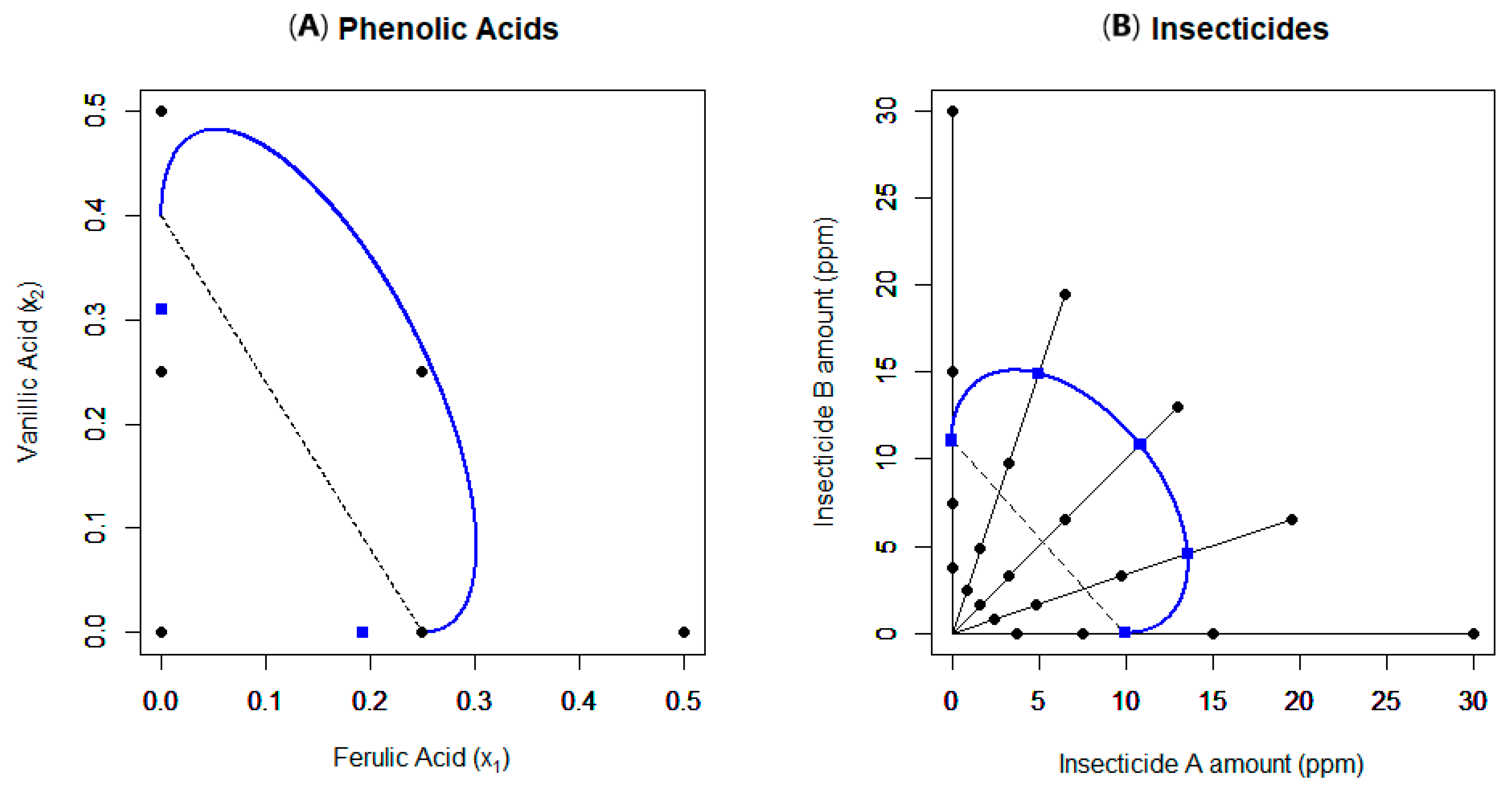
Figure 1. Isobologram plots for Examples 1 and 2. (A): Study of phenolic acids, six design support points (filled circles), estimated E C 50 points (filled squares), and curved isobole (partial elliptical curve) bowing out from the origin corresponds to the expected response for z = 0.25 with dashed line parallel to the independent action line. (B): Insect percent mortality for two insecticides. Ray design, with twenty design support points (filled circles), E C 50 points for insecticides A and B (filled squares along the horizontal and vertical axes), E C 50 line (dashed line), and 50% isobole.
Applsci 15 09971 g001
Figure 2. (A): Example 3 isobologram plot for aphid deaths and insecticides, two single-factor rays and one interior ray with 5–6 support points (filled circles) per ray, estimated E C 50 ’s (filled squares), and isobole exhibiting synergy. (B): Generic scatterplot for the Separate Ray model with the two one-at-a-time rays (Rays 1 and 2), interior Ray 3, and generic interior ray, Ray J. The E C 50 values at points C (compound B) and E (compound A). The E C 50 (thick-dashed) line intersects Ray J at the point D. The actual E C 50 along Ray J, on the thin-dashed line connecting points A and B, demonstrates synergy.
Applsci 15 09971 g002
Figure 3. Scatterplots of design support points (filled circles) and estimated L D 50 / E C 50 points (filled squares) using Separate Ray model fits to two 2 + 3 rays designs (i.e., with three interior rays) for Examples 4 and 5. (A): mice mortality cancer study of 6-mercaptopurine and amethopterin. (B): in vitro study of the effect of AZT (zidovudine) and ddI (didanosine) on reverse transcriptase viral activity. In both plots, the dashed lines represent the respective L D 50 / E C 50 lines.
Applsci 15 09971 g003
Figure 4. Scatterplots of Example 7 and 8 experimental designs, both involving In Vitro studies using five interior rays with chosen support points (filled circles) and fitted E C 50 or E D 25 points (filled squares). (A): radioactivity assessment and two oncology drugs; plate two results are shown here. (B): study of the effect of standard insulin (drug A) and A1-B29 suberoyl insulin (drug B) on the conversion of (3-3H) glucose to toluene-extractable lipids in rat fat cells. In both plots, the dashed lines represent the respective E C 50 / E D 25 lines.
Applsci 15 09971 g004
Figure 5. Scatterplots used to demonstrate the cut-line approach interaction assessment of web designs. (A): the two chosen cut line (dashed lines) and the 2 + 5 (five interior rays) web design, the points labeled P1–P7 show the intersection of the seven rays with the first cut line, the inner cut line. (B): the solid line connects the model-fit responses at the points P1 and P7, and the filled circles corresponding to the points which would be realized along this line for the five interior rays under the assumption/restriction of independent action. Filled squares are the actual observed responses for the five rays plotted above the number of each ray (R).
Applsci 15 09971 g005
Table 1. Summary of Chosen Examples.
Example
Number
Data Source
Reference
Experimental SetupModel(s) UsedFindingsNotes
1[8]Six support points; only one interior pointFinney 5 (normal); fixed & random chamber effectsAntagonismConsider adding more interior points and ray(s)
2[65]Ray design; 3 interior raysFinney 4b (binomial dist.)AntagonismGood design and spread of rays
3[67]Ray design; 1 interior rayFinney 4b (binomial dist.), separate slopesSynergyConsider adding more interior ray(s)
4[7]Ray design; 3 interior raysSR model; binomial distributionMixed; synergy for some raysAcceptable design; change ray slopes; use fewer support points per ray and increase n = 8
5[9]Ray design; 3 interior raysSR model; NB distribution (count data)Mixed; synergy for some raysGood design; change ray slopes for better spread
6[11]Ray design; 3 interior rays (two studies)SR model; binomial distribution Mixed; both synergy and antagonismGood design; use fewer support points per ray to increase n
7[66]Ray design; 5 interior rays; nine 96-well platesSR model; normal with random effects; model varianceSynergyGood design and spread of rays; reduce no. support points per ray
8[72]Web design; 5 interior rays; only 2 cut linesFinney and SR model with normal dist.(Marginal) antagonismReasonable design; consider using 4 cut lines (not two)
9[12]3 factors, non-ray design used due to practical limitationsExtended Finney model; binomial distributionPairwise synergy between all metal pairsThree-way combination (7th ray) should be added
10[74]3 factors, ray design with one interior ray per pair and the variable tripleExtended Finney and SR models; binomial distribution(Marginal) three-way antagonismConsider a larger study to increase power (i.e., increase chosen n = 10 )
Table 2. Potential Advantages and Disadvantages of the Finney, Separate Ray (SR) and Cut-line Combination Index (CLCI) Models.
ModelPotential AdvantagesPotential Disadvantages
Finney
  • Simple to fit using standard software
  • Often converges when other, richer models may fail to converge
  • Characterizes interaction with a single measure, which is often simple-to-interpret and to comprehend
  • Generally, does not involve overfitting the data
  • May provide too simple a model of the data and thus would exhibit significant lack-of-fit and perhaps an inaccurate interaction assessment
  • D-optimal design requires an efficient esti-mate of relative potency parameter (ρ), which in turn may entail a preliminary study to estimate ρ
SR
  • Entails (R − 2) interaction measures (parameters), richer model, may fit data when Finney model fails to do so
  • Often uses EC50s, estimation of which is often stable
  • May fail to converge due to too many model parameters relative to the chosen design
  • With (R-2) interaction parameters, may involve overfitting and require multiple comparison adjustment of type I error rate
  • Efficiently choosing interior ray slopes re-quires knowledge of ρ (relative potency) lest interior ray slopes fail to spread the design region
CLCI
  • With C cut lines and (R − 2) interior rays, entails C(R − 2) interaction measures (parameters), so may fit data when the SR and Finney models do not
  • Can detect interaction at other than 50% levels such as at 20%, 40%, 60%, and 80%, and these interaction assessments may differ
  • Whereas choosing the interior ray slopes requires knowledge of ρ, choosing the cut lines does not.
  • May fail to converge due to too many model parameters relative to the chosen design—even with a rich design
  • Choosing the design entails algebraic restrictions and thus calculations to find the ray/cut combination support points
  • With C(R − 2) interaction parameters, can easily involve overfitting, thus requiring adjustment of type I error rate for multiple comparisons (analogous to Scheffé’s adjustment for testing all contrasts)
  • Advantages of the CLCI model over the SR model is still unknown and needs to be demonstrated
Disclaimer/Publisher’s Note: The statements, opinions and data contained in all publications are solely those of the individual author(s) and contributor(s) and not of MDPI and/or the editor(s). MDPI and/or the editor(s) disclaim responsibility for any injury to people or property resulting from any ideas, methods, instructions or products referred to in the content.