APAED: Time-Optimized Adaptive Parameter Exponential Decay Algorithm for Crowdsourcing Task Recommendation

Abstract

The explosive growth of tasks on crowdsourcing platforms has intensified information overload, making it difficult for workers to spot lucrative bids; yet mainstream recommenders inherit a user-independence assumption from e-commerce and therefore overlook the real-time competition among workers, which degrades ranking stability and accuracy. To bridge this gap, we propose the Adaptive Parameter Exponential Decay Algorithm (APAED), which first produces base relevance scores with an offline neural model and then injects a competition-aware exponential decay whose strength is jointly determined by the interquartile range of each worker’s score list (global factor) and the live bid distribution of every task (local factor). This model-agnostic adjustment explicitly quantifies competitive intensity without handcrafted features and can be paired with any backbone recommender. Experiments on a real-world dataset comprising 25,643 tasks and 19,735 workers show that APAED cuts the residual RMSE of HR@10 from $9.575\times {10}^{-4}$ to $5.939\times {10}^{-4}$ (−38%) and that of MRR from $2.920\times {10}^{-4}$ to $0.736\times {10}^{-4}$ (−75%), substantially reducing score fluctuations across epochs and consistently outperforming four strong neural baselines. These results confirm that explicitly modeling worker competition yields more accurate and stable task recommendations in crowdsourcing environments.

1. Introduction

Crowdsourcing platforms are experiencing rapid growth in task volume, making it increasingly difficult for workers to identify promising bids. As system dimensions scale up, operational platforms—which encompass critical financial oversight systems like Sichuan University’s fiscal management platform—experience proportional increases in computational and network loads. This platform, representative of high-stakes financial operations, executes complex functions including high-volume transaction processing, multi-campus budget allocation tracking, and comprehensive year-end settlement calculations. These systems must reliably execute such complex, high-stakes tasks, demanding meticulous precision and extended processing cycles. This necessity underscores the critical requirement for highly efficient, dynamic resource allocation strategies that ensure robustness under load while simultaneously reducing time consumption. Such efficiencies are crucial to reducing the possibility of human errors in intricate financial tasks. While recommender systems have been deployed to relieve this information overload, most existing models inherit the user-independence assumption from e-commerce and media domains and thus fail to capture the fierce, real-time competition among workers for the same task. Consequently, the development of efficient, competition-aware task recommendation algorithms becomes paramount.

Recommendation algorithms for crowdsourcing are primarily categorized into two types [1]: one is the mainstream recommendation algorithm based on neural networks [2,3,4,5], and the other is the recommendation algorithm built on manual modeling for crowdsourcing scenarios [6,7]. Both types of algorithms exhibit deficiencies in crowdsourcing scenarios. Neural network-based recommendation algorithms typically employ single-point methods [4], pairing methods [8], or list methods [9] when generating output sequences. All three methodologies consider the interrelation of items based on the presumption of user independence. However, these algorithms overlook the non-independence of users in crowdsourcing scenarios, leading to inadequate recommendation accuracy. Manual modeling-based recommendation algorithms in crowdsourcing scenarios account for user non-independence, but they require extensive domain knowledge and human input, resulting in inferior learning and predictive capabilities compared to neural network-based methods. Therefore, no existing recommendation algorithm can simultaneously account for user non-independence, particularly in crowdsourcing scenarios deployed within mission-critical platforms like the Sichuan University Finance Office Management System where precision and reliability are paramount due to sensitive financial data and zero tolerance for errors, or exploit the learning and predictive strengths of neural networks, resulting in severely compromised recommendation accuracy and significantly reduced work efficiency. Therefore, this study aims to answer a research question that addresses the issue of inaccurate and inefficient recommendations caused by traditional recommendation algorithms failing to account for the non-independence among workers.

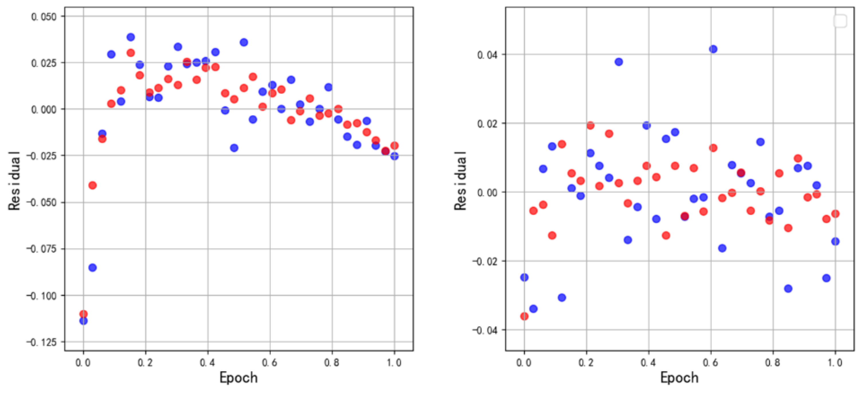
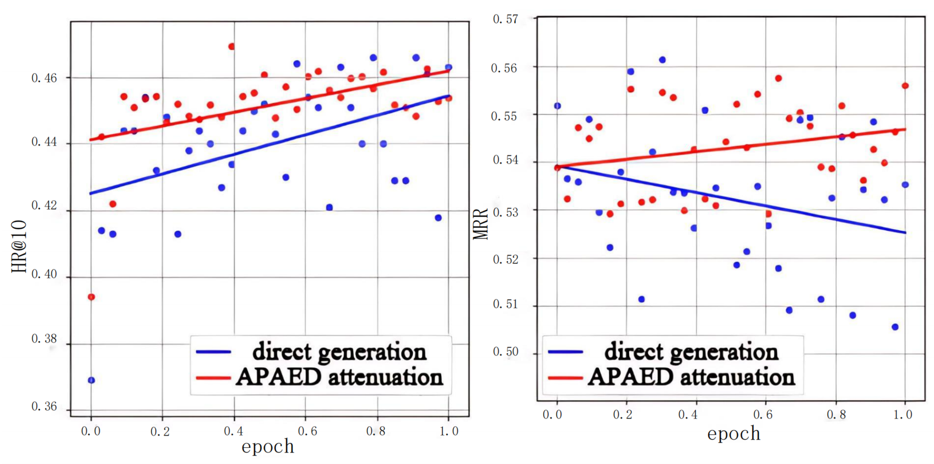
To address these issues, we propose an Adaptive Parameter Exponential Decay Algorithm (APAED) that factors in user competition. APAED introduces user non-independence into crowdsourcing scenarios by quantifying real-time competition among workers and uses it to adjust the prediction scores generated by the neural network model. This not only leverages the robust learning and predictive capabilities of neural networks but also factors in the effect of user non-independence on the score. Moreover, since the distribution of predicted values generated by the neural network model varies among different models, recommendation lists, and tasks, APAED incorporates an adaptive decay factor into the decay functions, enhancing its generalizability. By attenuating the prediction scores from the neural network model, APAED effectively resolves the issue of user non-independence without compromising the model, thereby improving the accuracy of recommendations and thus reducing processing time and enhancing system efficiency. Experiments show that APAED cuts the residual RMSE of HR@10 from $9.575\times {10}^{-4}$ to $5.939\times {10}^{-4}$ (−38%) and that of MRR from $2.920\times {10}^{-4}$ to $0.736\times {10}^{-4}$ (−75%), substantially reducing score fluctuations across epochs and consistently outperforming four strong neural baselines. The enhanced accuracy enables faster processing to improve workflow efficiency, while facilitating optimal task allocation to mitigate risks and better satisfy financial management system requirements.

The primary contributions of this study are as follows:

• The introduction of the Adaptive Parameter Exponential Decay Algorithm (APAED), an innovative recommendation algorithm that adjusts its decay factor adaptively based on the distribution of offline model predicted values. During the prediction process, APAED splits the worker’s tasks into an offline prediction part handled by the neural network model and an online prediction part managed by the APAED decay algorithm for score decay. The algorithm attenuates the score of the offline neural network model based on real-time competition intensity among workers, resulting in the final prediction.
• A comprehensive evaluation of APAED’s effectiveness using real-world datasets. The results demonstrate that APAED significantly improves relevant indicators compared to models that solely rely on neural networks and verify APAED’s robust generalization capabilities across different offline models. Our extensive experiments demonstrate the effectiveness and robustness of this strategy. When applied to the OPCA-CF backbone, APAED cuts the residual RMSE of HR@10 from $9.575\times {10}^{-4}$ to $5.939\times {10}^{-4}$ (−38%) and that of MRR from $2.920\times {10}^{-4}$ to $0.736\times {10}^{-4}$ (−75%), markedly reducing indicator fluctuations across training epochs. Similar gains hold for three additional neural baselines (NAIS, NAIS+AP, NAIS+DCA), where APAED lifts HR@10 and MRR by $15\sim 40\%$ on average while consistently tightening residual spreads. APAED marries the expressive power of deep recommenders with an explicit model of real-time worker competition, delivering state-of-the-art accuracy and stability for crowdsourcing task recommendation.

This paper is structured in the following manner: The Introduction segment elucidates the importance of this research and outlines the key contributions of this paper. The Related Work section offers a comprehensive review of existing research in the fields of crowdsourcing and recommendation algorithms. The section on the APAED Algorithm provides a detailed examination of the design and implementation of the APAED algorithm. The Algorithm Evaluation section uses real-world datasets to assess the performance and generalizability of the APAED algorithm. The Results section presents the data and descriptions of the experimental results, while the Discussion section discusses the main findings of the study as well as its limitations. Finally, the Conclusion summarizes the paper, encapsulating the key findings and their implications.

2. Related Work

This section provides an overview of recommendation algorithms as applied in crowdsourcing scenarios and discusses the utilization of decay functions in recommendation and other disciplines. Neural network-based recommendation algorithms can inherently decipher the implicit relationships among input time-series data or features in mainstream scenarios. This negates the need for an explicit application of decay functions, leading to their less frequent use in such algorithms. However, decay functions have numerous explicit applications in realms beyond recommendation. Consequently, this overview not only encapsulates the application of decay functions in recommendation scenarios but also extends to their extensive usage in various fields.

2.1. Recommendation Algorithms in Crowdsourcing Scenarios

Recommendation algorithms for crowdsourcing scenarios mainly include manual modeling methods and neural network algorithms.

Manual modeling methods in the crowdsourcing scenario requires a large number of manual features, such as modeling the worker’s completion probability and rate of return for the current task, modeling the possible remuneration of the publisher, and so on. Hossain MS et al. [10] used an association rule mining algorithm to generate a list of common skill sets used by workers in previous jobs, and also create feasible work lists based on workers’ common skills, customer ratings, minimum budget/hour rates, deadlines, etc. Kurup AR et al. [11] found that the participation rate and enthusiasm of new workers is higher than that of expert workers, so they distinguish skilled and unskilled workers through skill classification and the participation probability of existing expert workers, and recommend tasks separately.

Neural network in crowdsourcing scenarios is another approach. Pan Q et al. [12] employed Word2vec word vectors to calculate the tags used to characterize tasks and workers, and recommended tasks for workers by matching the similarity of tags between workers and tasks. The training sources for word vectors include historical bidding information and worker registration data. Liao Q et al. [13] proposed a role-based clustering model that permits each worker to bid in multiple task clusters and converts the entire worker–task evaluation matrix obtained from the worker’s history into a set of role-based, compact matrices. This not only achieves rapid system response but also mitigates the impact of irrelevant interactions. Shan C et al. [14] introduced reinforcement learning into crowdsourcing scenarios, using DQN (Deep Q Network) conjunction with neural networks to consider both long-term and short-term rewards, and can be updated in real-time to handle continuously updated data. Two DQNs are designed to capture the interests of workers and task issuers, optimizing the profit of the platform. Zhang D et al. proposed ApeGNN [15], a graph neural network (GNN) framework that dynamically adjusts aggregation weights for individual nodes in worker–task interaction graphs. By modeling local structural diversity (e.g., varying degrees of worker–task connectivity), ApeGNN achieves superior recommendation accuracy compared to static GNN models, particularly in sparse interaction scenarios. By leveraging a heterogeneous graph representation learning + reinforcement learning decision-making framework, Zhao B et al. [16] addresses the core challenges in spatiotemporal crowdsourcing, including dependency constraints, dynamic resource allocation, and large-scale generalization. Its innovation lies in modeling complex multi-task dependencies as a graph sequence decision problem and achieving efficient solutions through the dynamic embedding capability of CHANet, thereby providing a theoretical foundation and practical tools for industrial-grade crowdsourcing platforms. Chiang J-H et al. [17] integrates lifecycle modeling, context-aware computing, and the attention mechanism to address issues such as user interest drift and insufficient scenario adaptation in traditional recommendation systems.

From the literature, it is apparent that manual modeling methods in crowdsourcing scenarios heavily lean on artificial domain knowledge, resulting in a model that lacks generalizability and has poor reproducibility. The neural network method does not account for the non-independence among workers, leading to a decline in the accuracy of recommendations. This is particularly important for platform environments requiring refined financial oversight, such as the Sichuan University Finance Office, to minimize redundant bidding and resource waste.

2.2. Decay Algorithm

Medo M et al. [18] proposed an adaptive model that melds the similarity of user rating patterns with the popular dissemination of news on the evolving network. This model measures user similarity through the positive and negative feedback of users to news, facilitating novel news recommendation through the decay of recommendation scores over time. At each time step, the news score in the user recommendation queue decays, and when the attenuated score drops below a certain threshold, it is removed from the recommendation queue. Anelli V M et al. [19] introduced the popularity of items into the collaborative filtering algorithm and proposed the Time Pop algorithm. This algorithm does not consider global popularity, but regards the popularity of items among the user’s neighbors, avoiding the use of time windows and fixed number of tags when selecting candidates. Zheng Q et al. [20] introduced an improved collaborative filtering algorithm based on expert trust and time decay. The expert group is obtained through expert trust, and the similarity between the expert and the target user is used to calculate the weight of the expert’s rating. The predicted value of the target user is obtained through the user’s weighted level and time decay factor. Peng D et al. [21] also presumed that user interests in social networks were in a state of constant flux, thereby improving the single forgetting function algorithm.

Applications of the decay functions beyond the context of recommendation include the following: Yue Shubo et al. [22] studied the decay law of surge waves that changes with the initial shape determined by the water entry angle, speed, and height of a landslide body through sinusoidal decay. Yuan Zhihui et al. [23] used the tangent function of the principal stress of the original and reshaped loess introduced in the Nth dry–wet cycle to describe the shear strength decay value of the original and reshaped loess after the dry–wet cycle. Feng Shuai et al. [24] used the river activity coefficient, the average flow velocity of the river, and the average water depth to modify the comprehensive decay coefficient of the first-order reaction kinetics. The comprehensive decay coefficient is a basic logarithmic function composed of the pollution concentration and time before and after the decay. By leveraging a personalized temporal decay function and dynamic collaborative filtering, Ghiye A et al. [25] addressed the issue of interest drift in financial recommendation systems, which is caused by data non-stationarity and user heterogeneity. Its core innovation lies in extending the decay mechanism from global parameters to the user level, and achieving efficient adaptation through incremental learning. Chen X et al. [26] systematically revealed the core role of Weight Decay in the sparsification of neural networks and proposed an innovative method to achieve efficient and low-loss end-to-end compression.

3. APAED Algorithm

The APAED algorithm stands as the pioneering crowdsourcing recommendation model that integrates offline model predictions with real-time bidding dynamics to quantitatively evaluate the competitive intensity of present tasks in crowdsourcing environments. APAED employs both global and local distributions of predicted values to derive decay parameters, serving to attenuate these predicted values. Within APAED, decay and gain function symmetrically, yet our discussion will solely focus on the process of establishing decay parameters. This is predicated on the assumption that the primary influence on a worker’s bidding success stems from competition-induced decay. Consequently, the decay parameter, embodying real-time competition data, is adjusted to impact the gain at the end. The APAED accounts for the non-independence among staff members, thereby more effectively mitigating resource waste and enhancing work efficiency on high-pressure platforms, especially in systems with stringent task efficiency requirements such as Sichuan University’s Financial Management System.

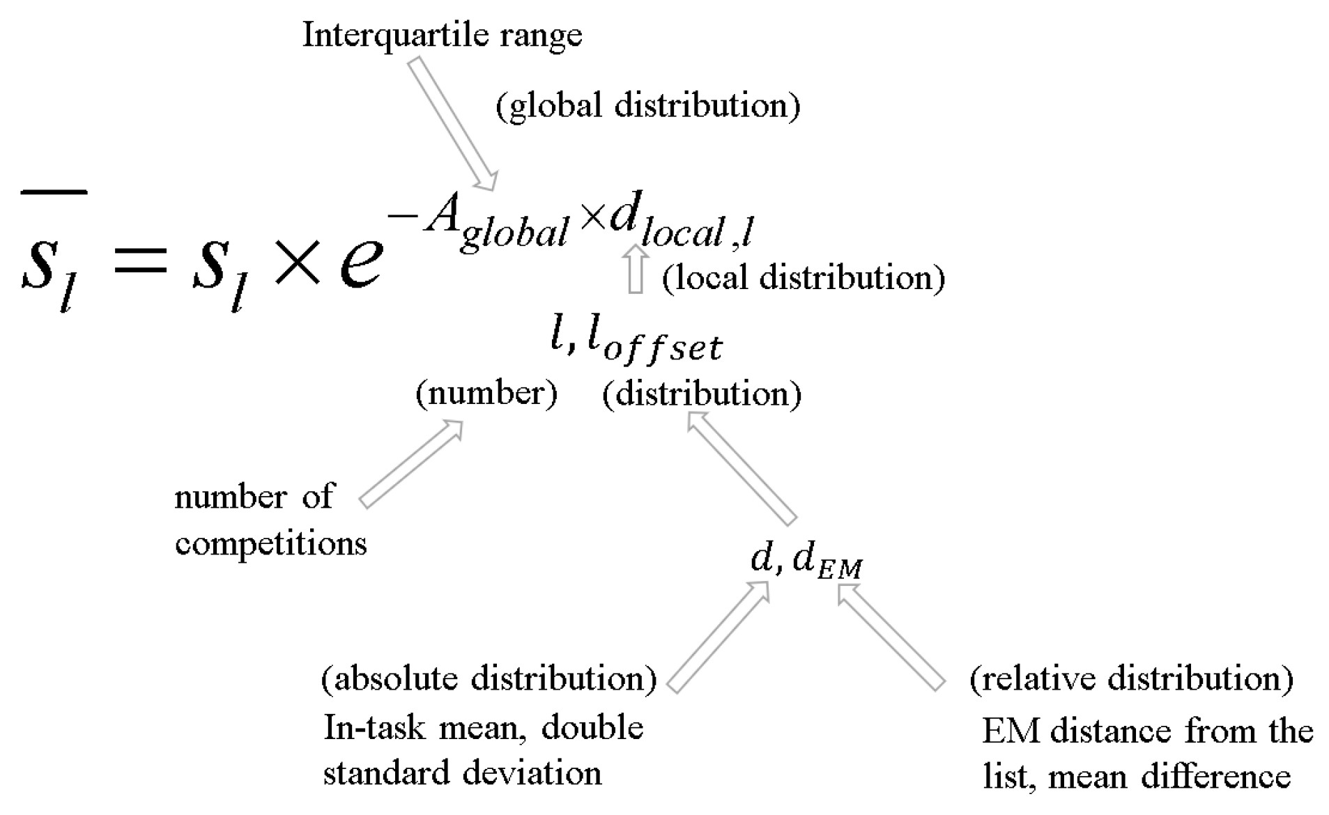
When attenuating the predicted value, APAED will determine the decay or gain parameters from the predicted value distribution from two angles, which are the global distribution and local distribution of the predicted value, respectively. The global distribution is the distribution of the predicted value of the entire list when the recommendation list is generated for a certain worker, and the local distribution is the distribution of the predicted value of a task in the recommendation list. When generating the recommendation list, since only the predicted value of the current bid is known, the competition information is only reflected based on the record of the bid. The relationship between the global and local decay functions and the final decay functions, and the standards involved are shown in Figure 1. In this figure, $\overline{s_l}$ is the final recommendation score after decay adjustment by the APAED algorithm while the $s_l$ represents the initial recommendation score generated by the offline neural network model for the l-th task. $A_{global}$ denotes the global decay factor, calculated based on the interquartile range of the recommendation list as shown in Formula (2). $d_{local,l}$ refers to the local decay factor for the l-th task, which is determined by factors such as the number of bids, absolute score distribution, and relative score distribution of the task, and is used to adjust the decay magnitude of the recommendation score for that task, as illustrated in Formula (3). The exponential decay formula integrates global and local information, enabling the recommendation results to align with both the historical preferences of workers and the real-time competitive environment, thereby enhancing the accuracy and stability of task recommendations. A more detailed exposition of the parameters l, $l_{offset}$d, and $d_{EM}$ will be provided in subsequent sections.

3.1. Offline Prediction Model

In this research, NAIS [27] is used as the framework of the offline model, and the APAED algorithm is used to attenuate the offline prediction value generated by the offline model. You can find more details about NAIS in the “Comparison of Algorithms” section referenced in Section 4. Because the tasks in crowdsourcing are time-sensitive and cannot directly use the id in NASI as feature input, here we follow the method of learning news features according to news attributes in NEWS [28], and learn crowdsourcing features according to the attributes of crowdsourcing tasks.

3.2. Global Decay Parameter

The predicted value after decay $\overline{s}=[\overline{s_1},\overline{s_2},\dots ,\overline{s_l}]$ is shown in Formula (1). The decay object here is all the predicted values of the worker in the list when the recommendation list is generated for a certain worker $s=[s_1,s_1\dots ,s_l]$, where l is the number of tasks in the list.

$${\overline{s}}_l=s_l\times e^{-{\alpha }_{global}\times d_{local,l}}.$$

(1)

In Formula (1), ${\alpha }_{global}$ is used as a global decay factor to determine the influence of the distribution of predicted values in the entire recommendation list on the decay intensity.

Because the purpose of decay is to adjust the relative position ranking of the predicted value $s_l$ of each task in a certain worker s according to the competition information, and ${\alpha }_{global}$ as a global decay factor determines the upper limit of the decay strength for changing the relative ranking position, ${\alpha }_{global}$ is thus determined by the overall distribution of s. When the value of s is more discrete, a greater decay strength ${\alpha }_{global}$ is needed to affect the relative position ranking in s.

Use the interquartile range $Q=Q_1-Q_3$ of s as the benchmark for ${\alpha }_{global}$. The interquartile range is mainly used to measure the degree of dispersion of the predicted value of the worker recommendation list. It reflects the degree of dispersion of the middle 50% of the data, calculated as the difference between the upper quartile (Q3, which is located at 75%) and the lower quartile (Q1, which is located at 25%). The interquartile range can avoid the influence of extreme values, because after OPCA-CF prediction, the smallest extreme value in each recommended list tends to 0, and the largest extreme value tends to 1, which does not reflect the degree of dispersion of the data. ${\alpha }_{global}$ can make the list position shift caused by the decay of $s_l$ within the task up to 50%, that is, attenuate from $Q_3$ to $Q_1$. Define ${\alpha }_{global}$ as the intensity required to attenuate $Q_3$ to $Q_1$ using exponential decay, which is obtained by Formula (2):

$$Q_1=Q_3\times e^{-A_{global}}\to A_{global}=-log \left(\frac{Q_1}{Q_3}\right).$$

(2)

3.3. Local Decay Parameter

Local decay parameter $d_{local,l}$ is used as the local decay factor in each task, which represents the influence of the predicted value $s_l=[s_l,s_{l1},s_{l2},\dots ,s_{lm}]$ of other workers in the l-th task on the decay intensity. m is the predicted value of other workers’ bid records in the l-th task. $d_{local,l}$ is determined by the Formula (3). The parameters l, d, and $d_{EM}$ will be explained below.

$$d_{local,l}=f(l,d,d_{EM}).$$

(3)

3.3.1. Bid Quantity Parameter ${\Delta }_l$

A bidding behavior greater than the predicted value of $S_l$ in a task will strengthen the competition of the current task and cause the decay of $S_l$. Since the upper limit of the decay strength is ${\alpha }_{global}$ determined by the global distribution, it is hoped that ${\Delta }_l$, determined by the number of bids, can tend to 1 when the competition is strongest, so that the final decay strength can be between 0 and ${\alpha }_{global}$. Here, ${\Delta }_l=tanh(l_0\times l\times l_{offset})$, where $l_{offset}$ is used to map the number of bids to a range that makes $tanh$ meaningful, and $l_0$ is a hyperparameter defined according to the magnitude of the bid.

3.3.2. Parameter d, $d_{EM}$ Determined by the Absolute Distribution of the Predicted Value of the Bid Within the Task and the Relative Distribution of the Predicted Value Between the Lists

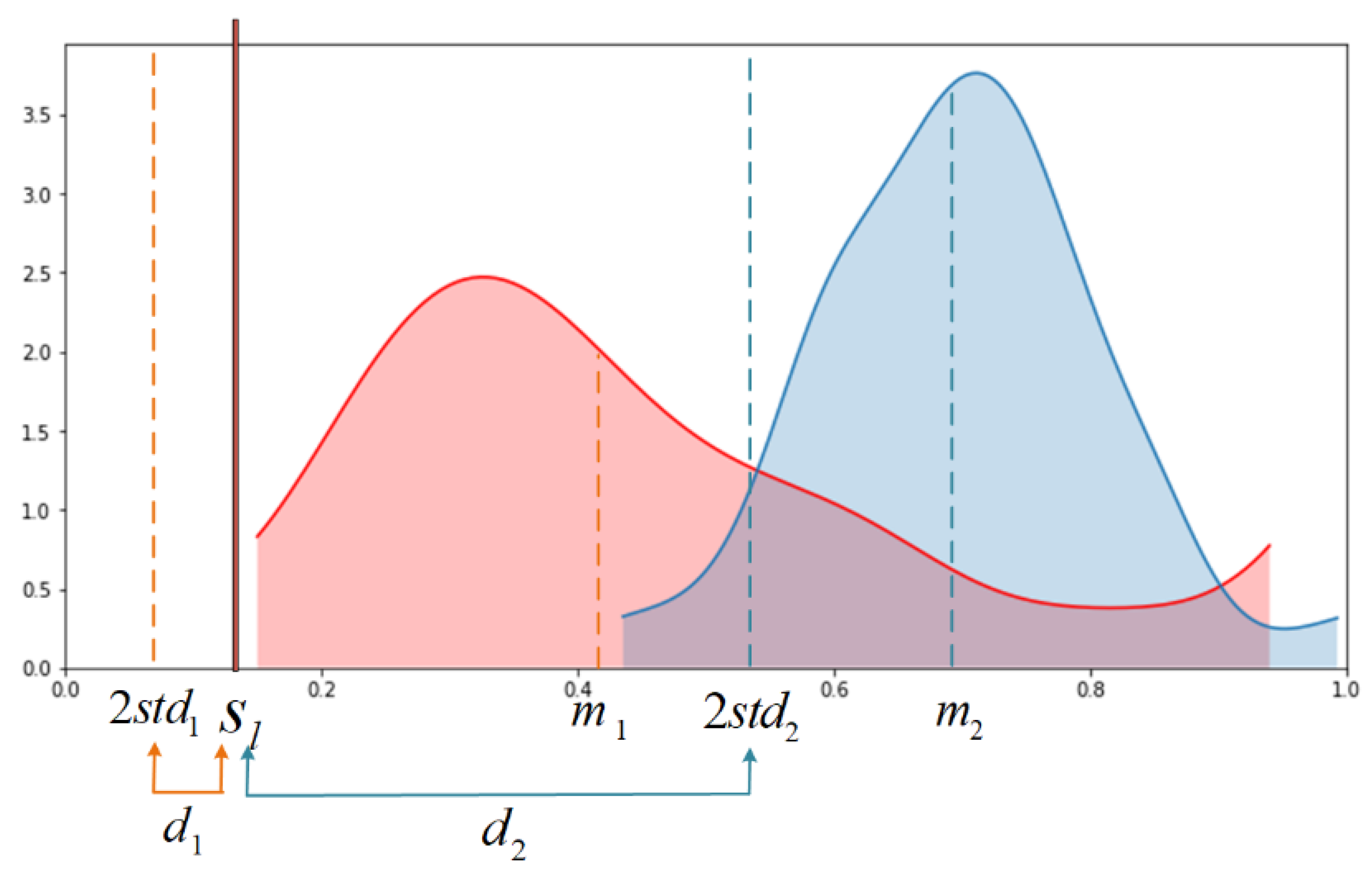
In addition to the influence of the number of bids on the decay intensity, the distribution of $s_l=[s_l,s_{l1},s_{l2},\dots ,s_{lm}]$ will also affect the current decay intensity, which can be used to correct $l_0$. In the case of the same number of bids, different $S_l$ distributions will also cause different decay strengths. As shown in Figure 2, the blue and red shades represent the two types of predicted value density distributions with the same bid quantity but different distributions. Obviously, the decay intensity of the blue distribution to the predicted value is greater than that of the red distribution.

Therefore, d is introduced here to indicate the distance between $S_l$ and $S_l$ by two standard deviations, $d\in (-1,1)$. In this way, d is determined by the degree of concentration and dispersion of $S_l$. Obviously, the blue part in Figure 2 causes a greater degree of competition than the red part, so $d_2>0>d_1$.

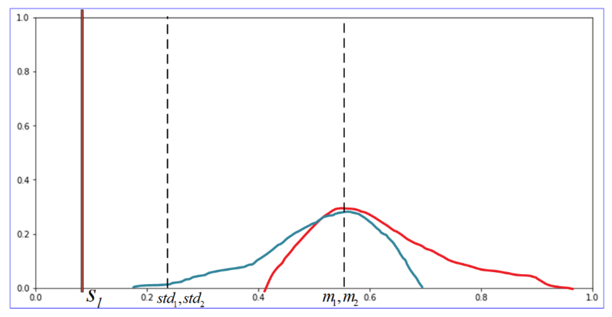
In addition to the distance d between the distribution and the current predicted value $S_l$, the shape of the distribution itself will also cause differences in the intensity of competition, and d only includes the mean and variance of the data and cannot reflect the shape of the distribution. Because the predicted value does not necessarily conform to the normal distribution, there may be information where the mean and variance are the same but the competition intensity is different. As shown in Figure 3, the blue and red distributions have the same mean and variance, that is, s is the same, but obviously the red distribution represents greater competition.

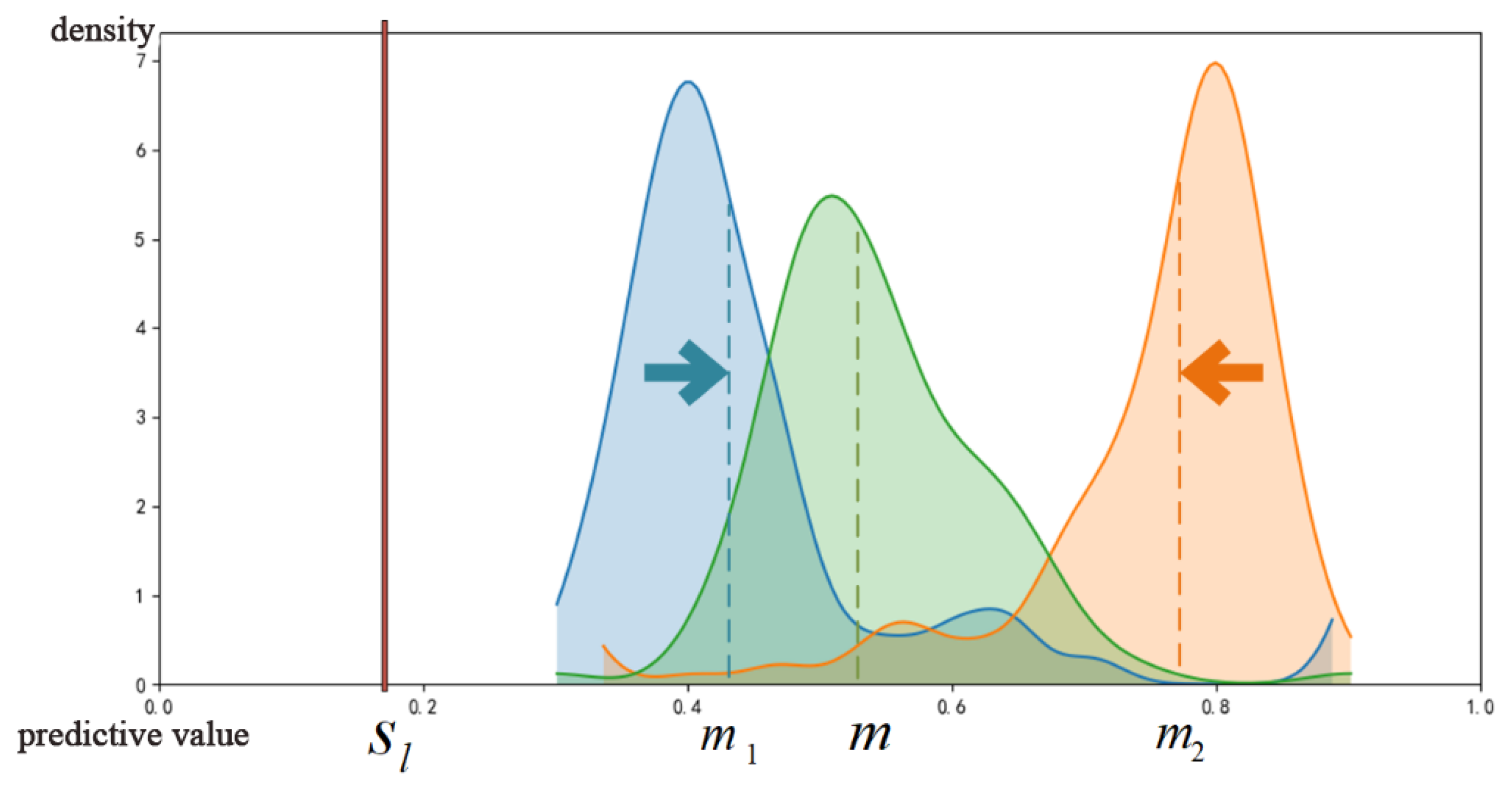
Therefore, d needs to be strengthened or suppressed according to the distribution pattern. In order to determine whether to strengthen or suppress and perform quantitative analysis, it is necessary to use a certain distribution as a benchmark. Here, we use the prediction value distribution $slist[minima:maxima]$ of the current recommendation list between the extreme values of $S_l$ as the benchmark, as shown in the green part of Figure 4. Then, we use EMD (Earth Mover’s Distance) to calculate the distance from distribution $S_l$ to $S_{list}$ in the task, which is obtained by Formula (4).

$$W(s_l,s_{list})=\underset{\gamma \sim \prod (s_l,s_{list})}{inf}{E}_{(x,y)\sim \gamma }[\Vert x-y\Vert ]$$

(4)

where $\prod (s_l,s_{list})$ is the set of all possible joint distributions that combine the two distributions. For each possible joint distribution, samples x and y are obtained from it, and the distance of the pair of samples and the expected distance $E_{(x,y)\sim \gamma }[\Vert x-y\Vert ]$ of all samples are calculated. The lower bound of this expected value in all possible joint distributions is from $S_l$ to $S_{list}$, the EM distance.

Intuitively, the EM distance is to imagine the probability distribution as a pile of dirt. In Figure 4, the task distribution (blue and red parts) moves in the direction of the arrow, and the energy required to pile it into another target shape $s_{list}[minima$:$maxima]$ (green part) is determined by carrying out the minimum amount of work.

In order to avoid the influence of the predicted value dimension on W, it is necessary to normalize $S_l$ and $S_{list}$ before calculation because the dimension of the local predicted value is unrelated to the decay intensity caused by the predicted value distribution; for example, $S_l$ and $S_l$ are both in the order of magnitude $1^{-3}$ and $1^{-1}$, and the intensity of competition faced by $S_l$ is the same. Subsequently, since the EM distances are all greater than zero, it is impossible to determine whether to strengthen or suppress d. Here, the mean difference between $S_l$ and $S_{list}$ is used as the standard for strengthening or suppressing. If it is positive, it will be strengthened, and if it is negative, it will be suppressed, that is, $m_1-m$ and $m_2-m$ in Formula (5). Finally, the decay caused by the distribution of the predicted value is shown in Formula (5).

$$d_{EM}=sigmoid(mean\left(s_l\right)-mean\left(s_{list}\right))\times e^{W(s_l,s_{list})}.$$

(5)

Finally, d and $d_{EM}$ jointly determine $l_{offset}$, as shown in Formula (6).

The improved sigmoid function is used here, and the sigmoid function can be used to avoid the occurrence of outliers leading to excessive changes in $l_0$, $g(d,d_{EM})\in (0.5,1.5)$. ${\mu }_1$ and ${\mu }_2$ are used as hyperparameters to scale and correct the overall intensity.

$$l_{offset}=g(d,d_{EM})={\displaystyle \frac{1}{1+e^{-{\mu }_{1}d\times e^{{\mu }_2\times d_{EM}}}}}+0.5.$$

(6)

Finally, use a symmetrical method to calculate the gain part of $S_{lm}<S_l$. The gain here is not to increase $S_l$, but to weaken $S_{lm}>S_l$ obtained by $d_{local,l}$. For example, even if the competition intensity is the same, the probability of winning the bid of $S_l$ in the top 10% and the bottom 10% of the task is obviously different. The part $S_{lm}>S_l$ should be used to adjust $d_{local,l}$, and $d_{local,l}$ will be suppressed as the gain increases. Here, it is believed that the importance of decay is greater than the gain in competition, so the local distribution gain parameter $g_{global,l}$ obtained by the symmetric method is penalized. After obtaining $g_{global,l}$, we use the ratio $r_1$ of $g_{global,l}$ to $d_{local,l}$ to weaken $d_{local,l}$, the sigmoid function to smooth $r_1$, and cosine decay to obtain the final local decay parameter $d_{local,l}$, as shown in Formula (7).

$$d_{local,l}=d_{local,l}\times cos(2\times (1/(1+e^{-r_l\beta })-0.5)).$$

(7)

Among them, $\beta$ is the maximum suppression ratio of the hyperparameter control gain part to $d_{local,l}$.

The purpose of using the cosine function is that even if the decay reaches the maximum, that is, when $r_1=1$, $d_{local,l}$ will not be attenuated to 0, so as to ensure that the decay is dominant in competition.

4. Algorithm Evaluation

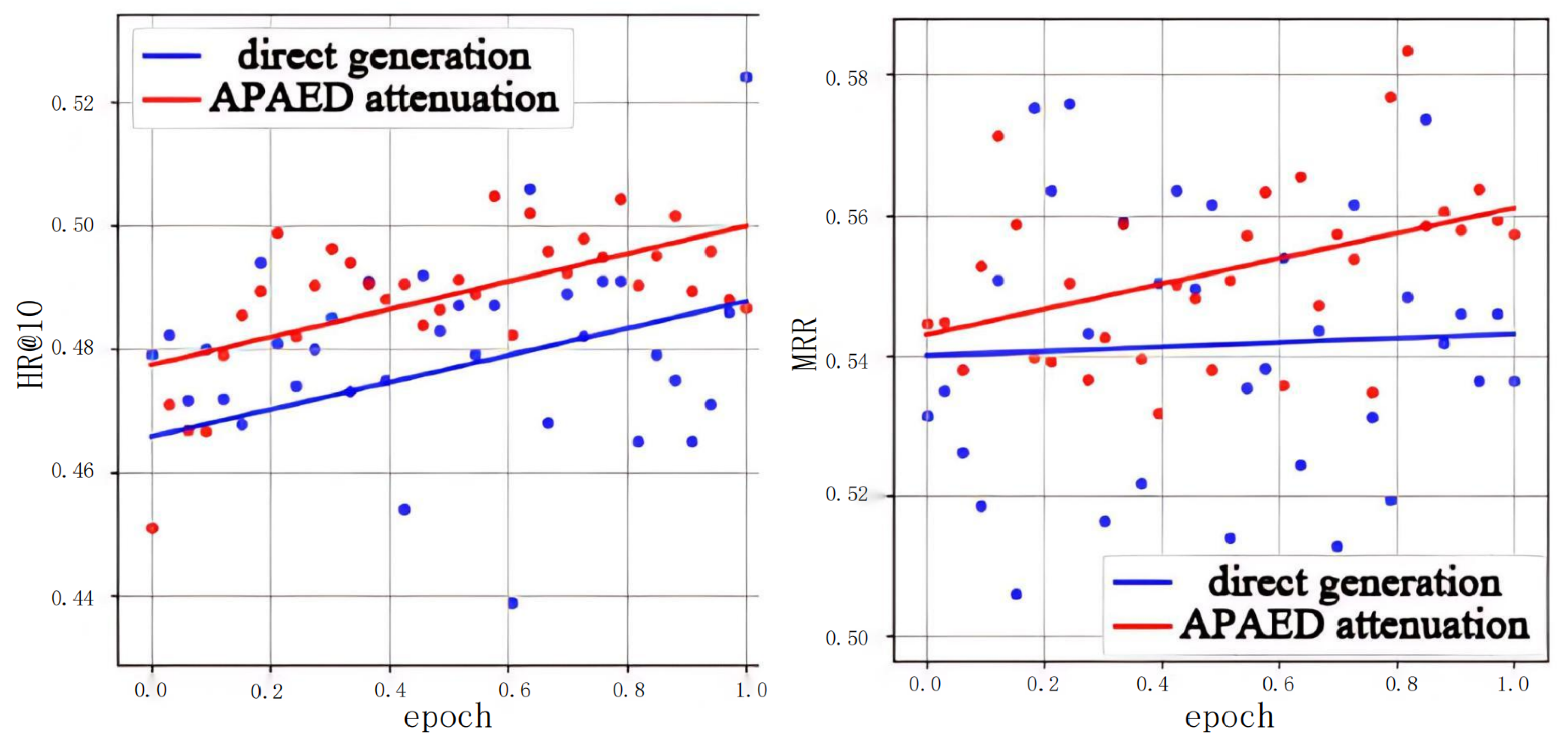
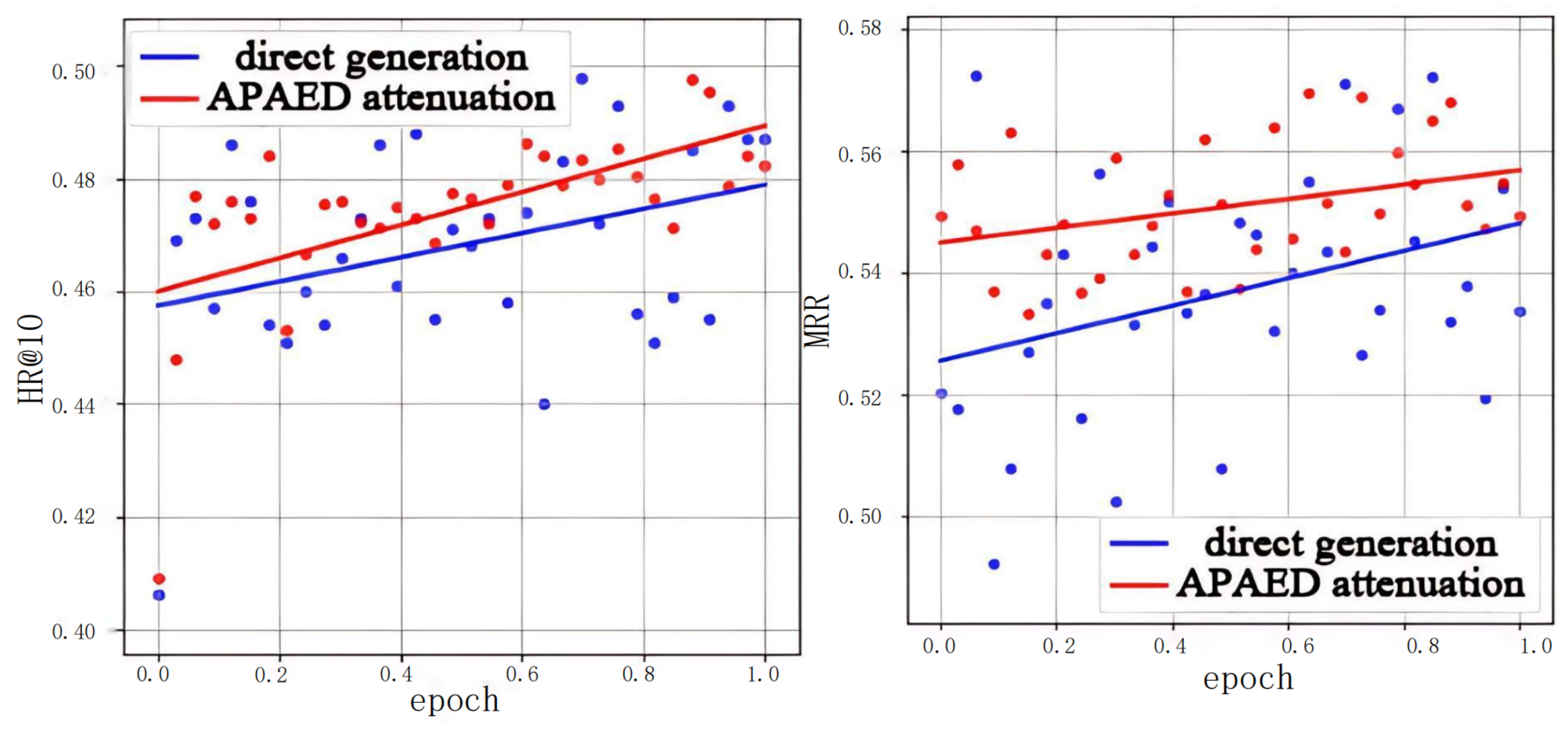
The experiment in this research compares the difference between the recommendation list directly generated by the offline model and the recommendation list generated using the APAED algorithm in indicators HR@10 and MRR, which proves that the APAED algorithm has an inhibitory effect on the abnormal fluctuation of the indicators in the crowdsourcing scenario.

• Dataset and experimental environment:

The experimental environment used comprised Windows 10 Professional 64-bit, Intel Core i7-8700 @ 3.20 six-core, NVIDIA Geforce RTX 2060 (6 GB). The algorithm was built by tensorflow 1.13.1 and python 3.6.8.

The filtered dataset statistics are shown in

Table 1. Dataset statistics.

Number of Samples	Number of Tasks	Number of Workers	Number of Publishers	Number of Winning Bids
513,612	25,643	19,735	17,340	52,351

. There were 963,352 pieces of original data before filtering. It can be seen that half of the workers on the original website have never won the bid without a personalized recommendation algorithm.

• Evaluation indicators:

This research compares the difference between the recommendation list directly generated by the offline model and the recommendation list generated using the APAED algorithm in indicators HR@10 and MRR, and uses a straight line to fit the fluctuation curve of HR and MRR with epoch, uses Root Mean Squared Error (RMSE) as the loss function, and trains 8000 steps with the SGD optimizer. The training residual can reflect the intensity of the fluctuation.

• Comparison algorithm:

In order to verify that the APAED algorithm can improve the indicators related to the recommendation list and test the generalization ability of the algorithm among different offline models, we need different offline models to generate different offline prediction value distributions. However, most of the existing neural network algorithms cannot be directly applied to crowdsourcing. Therefore, the offline model adopts a fixed main network and changes the attention sub-network to generate different offline prediction value distributions. Four attention mechanisms are selected here.

NAIS: In this experiment, tasks are used instead of Item, and workers are used instead of User. Taking the sequence of workers as an example, the attention mechanism is shown in Formula (8). In this formula, $g_i^{\prime }$ represents the feature embedding vector of the i-th task historically interacted with by the target worker, such as task type, reward, deadline, etc. r denotes the worker embedding vector of the target worker g. $g^{\prime }\odot r$ represents the element-wise product between the worker embedding vector and the task embedding vector, capturing the matching degree between the task and the worker’s preferences or capabilities. $W_g$ is a $d\times d$-dimensional matrix used for a linear transformation of features. $ReLU$ serves as the activation function, filtering out negative signals while retaining positive matching features. $h_g$ is the output weight of the attention network with a dimension of $d\times 1$, which projects the worker–task matching features into a scalar weight. $b_g$ is the bias term of the network, applied to correct scoring errors. L represents the total number of tasks, that is, the number of tasks in $f^{\prime }$, which controls the calculation range of max-pooling to ensure coverage of all possible task matching items. After normalization, the attention weight $a_{i,j}$ for the i-th task encountered by the worker is obtained. The greater this weight, the higher the reference value of this historical task for the current recommendation.

$$a_{g,i}={\displaystyle \frac{exp\left(g(g_i^{\prime },r)\right)}{{\displaystyle \sum _{j=1}^L}exp\left(g(g_j^{\prime },r)\right)}},g(g^{\prime },r)=h_g^{\mathrm{T}}RELU(W_g(g^{\prime }\odot r)+b_g).$$

(8)

Attentive pooling networks [29] (hereinafter referred to as AP): Since its model is designed for QA (question and answer), in the experiment, it is used to replace the attention mechanism part of NAIS (hereafter replaced by NAIS+AP). Taking the worker sequence as an example, the attention mechanism is shown in Formula (9). In this formula, $g^{\prime }$ denotes the worker-side original feature matrix with dimensions corresponding to the number of workers × worker feature dimensions, including features such as workers’ historical completion rates and specialized task types. $G^{\prime }$ is the worker feature projection matrix that compresses high-dimensional original worker features into a low-dimensional embedding space, with dimensions of target embedding dimension × worker feature dimensions. $f^{\prime }$ stands for the task-side original feature matrix with dimensions of number of tasks × task feature dimensions, including attributes such as task rewards, difficulty levels, and deadlines. $F^{\prime }$ is the task feature projection matrix that functions similarly to $G^{\prime }$ and compresses high-dimensional task features into a space with the same dimension as the worker embedding. U is the cross-feature attention weight matrix for workers and tasks with dimensions of target embedding dimension × target embedding dimension, whose core role is to capture high-matching interaction relationships between worker and task features. $G^{\prime }\left(g^{\prime }\right)$ is the low-dimensional embedding matrix of original worker features projected by $G^{\prime }$, where each row corresponds to the embedding vector of one worker. $F^{\prime }{\left(f^{\prime }\right)}^T$ is the transpose of the embedding matrix of original task features projected by $F^{\prime }$, where each column corresponds to the embedding vector of one task. M is the worker–task interaction score matrix with dimensions of number of workers × number of tasks. The element $M_{j,m}$ represents the matching score between the j-th worker and the m-th task. After tanh activation, its value range is $(-1,1)$, and a larger value indicates a higher matching degree. $a_{g,j}$ is the maximum matching weight of the j-th worker for the target task g, obtained by taking the maximum value of the scores $M_{j,m}$ between this worker and all tasks, and used to screen the contribution of task features most suitable for the worker.

$$a_{g,j}=\underset{1<m<L}{max}\left(M_{j,m}\right),M=tanh\left(G^{\prime }\left(g^{\prime }\right)U{F}^{\prime }{\left(f^{\prime }\right)}^T\right).$$

(9)

The collaborative attention mechanism used in ref. [30]: Since the matrix dot product is used in the attention mechanism, it is referred to as DCA (Dot Co-Attention), which replaces the attention mechanism part of NAIS, hereinafter referred to as NAIS+DCA. Take the worker sequence as an example of the attention mechanism, as shown in Formula (10). $g^{\prime }$ is the low-dimensional feature embedding vector of the target worker with dimensions of target embedding dimension × 1. $f^{\prime }$ is the low-dimensional feature embedding vector of the target task with the same dimension as $g^{\prime }$. $W_{gg}$ is the self-attention weight matrix on the worker side with dimensions of target embedding dimension × target embedding dimension. $W_{gf}$ is the cross-side attention weight matrix between workers and tasks with the same dimension as $W_{gg}$. After tanh activation, their value range is $(-1,1)$, which avoids gradient explosion and highlights valid features. $h_g$ is the worker–task bidirectional feature fusion vector obtained by element-wise multiplication of the above two activation vectors. $W_g$ is the fusion feature output weight matrix with dimensions of number of candidate recommended tasks K× target embedding dimension. It is used to project the high-dimensional fusion vector into K-dimensional candidate task scores. $b_g$ is the output layer bias term with dimensions of K× 1. It is used to correct the baseline bias of projected scores and avoid overall score deviation caused by uneven feature distribution. $a_g$ is the attention weight distribution of the target worker for candidate tasks. After Softmax normalization, its value range is $(0,1)$ and the sum is 1. A higher weight for a task indicates a stronger willingness of the worker to accept it, leading to a higher ranking in the recommendation list.

$$a_g=softmax(W_g{h}_g+b_g),h_g=tanh\left(W_{gg}{g}^{\prime }\right)\odot tanh\left(W_{gf}{f}^{\prime }\right).$$

(10)

The collaborative attention mechanism is used in this article, and it is also used to replace the attention mechanism part of NAIS, hereinafter referred to as OPCA-CF.

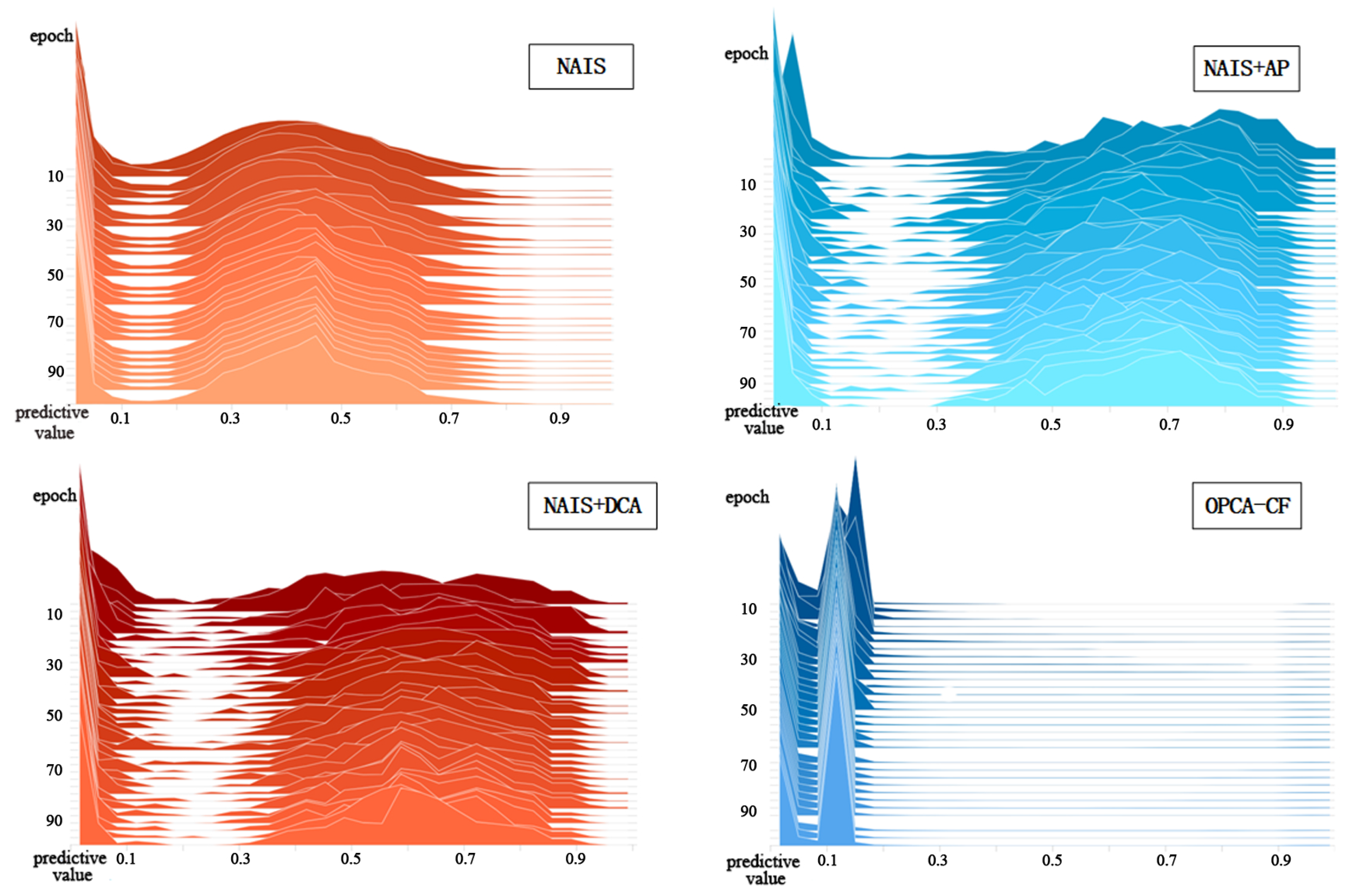
The distribution of predicted values generated by the four offline models is shown in Figure 5. It can be seen that replacing the sub-network can meet the requirements of generating different predicted value distributions.

5. Results

The HR@10 and MRR of using and not using APAED to generate the recommendation list after obtaining the offline predicted value are shown in Figure 6 (normalized epoch to 0 to 1).

On the HR@10 and MRR indicator graphs, the red part represents the offline predicted value considering worker competition. It can be seen that HR@10 decreased from $9.575\times 1^{-4}$ to $5.939\times 1^{-4}$ on the RMSE, and MRR decreased from $2.920\times 1^{-4}$ to $0.736\times 1^{-4}$ on the RMSE, which effectively alleviated the abnormal fluctuation of the recommendation list. The residuals of HR@10 and MRR linear fitting are shown in Figure 7. It can be seen that the residuals in the red part (after APAED decay) are more concentrated on the x-axis, that is, more stable.

After the other three comparison models use the APAED algorithm to generate the recommendation list, the corresponding indicators are also more stable and improved. The HR@10 and MRR of NAIS, NAIS+AP, and NAIS+DCA before and after using APAED and their linear fitting residuals are shown in Figure 8, Figure 9 and Figure 10 (the red dotted line indicates after using APAED).

The RMSE of each model’s linear fitting loss before and after using APAED is shown in

Table 2. APAED super-parameter table for each model.

	Directly Generated List		APAED-Generated List
	HR@10	MRR	HR@10	MRR
OPCA-CF	9.575	2.920	5.939	0.736
NAIS	2.358	3.427	0.789	1.229
NAIS+AP	2.857	3.295	1.399	0.885
NAIS+DCA	3.075	2.245	1.215	0.726

. After using APAED, the RMSE of each model decreases, and the residual error is more concentrated on the x-axis, which suppresses the fluctuation of the relevant indicators of the recommendation list. It can be seen that APAED has the generalization ability between the offline predicted values generated by different models.

Parametric Comparison and Hyperparameter Search

Here, we present the comparative experiments conducted on the determination of hyperparameters and use control variables to verify the necessity of the global decay factor determined by the global distribution and the local decay factor determined by the local distribution in APAED. OPCA-CF is selected as the offline model.

As shown in Figure 11, the comparison of different $l_0$ values on HR@10 and MRR indicators is shown (the base curve is the corresponding hyperparameter set in Table 2), whereby $l_0$ determines the initial strength of the local decay within the task. It can be seen that if $l_0$ is set too small, it will be impossible to change the partial order of scores in the worker list, and too large a value will result in greater fluctuations.

Figure 12 shows the comparison of different parameters on HR@10 and MRR indicators, respectively. ${\mu }_1$ determines the decay strength of the local decay factor within the task determined by the distance between the predicted value in the task and the predicted value of the current worker, and determines whether $l_0$ is a gain or suppression, that is, the decay strength caused by the absolute distribution of the predicted value within the task.

Figure 13 shows the comparison of HR@10, HR@10, MRR, and MRR residuals, respectively. ${\mu }_2$ determines the gain or suppression strength of ${\mu }_1$ to $l_0$. It can be seen that when ${\mu }_2$ is large, the list position shift is large, which results in poor suppression of fluctuations. On the contrary, when ${\mu }_2$ is small, the strength of the list shift is small.

Finally, an experimental comparison is conducted on the gain part to compare whether it is necessary to introduce a higher score than the current worker’s predicted value to suppress the decay intensity. The comparison before and after the introduction of suppression is shown in Figure 14. It can be seen that when quantifying the intensity of competition based on the online real-time bidding information, both higher scores and lower scores than the current worker’s predicted value should be considered.

6. Discussion

To address the question concerning the failure of traditional models to account for the interrelationships among workers, we incorporated real-time competitive relationships among workers into the algorithm we designed. We propose the APAED algorithm as an online tool. The prediction model attenuates the offline prediction value according to the real-time competition information, and improves the relevant indicators while mitigating fluctuations. The experimental results show that APAED achieves better performance compared with traditional algorithms that directly generate recommendation lists, and Figure 12, Figure 13 and Figure 14 also indicate that the model has good robustness under different hyperparameters. However, in the Results section, we only used the indicator data of HR@10 and MRR for the results in a simplistic manner, without conducting more rigorous statistical analyses. This is a limitation of our study, and we will perform detailed statistical analysis in our subsequent research.

7. Conclusions

In order to ensure that the model uses high-quality feature expressions and prediction capabilities of the neural network model while taking into account real-time competition, this research uses neural network algorithms such as OPCA-CF as an offline prediction model, and on this basis, proposes the APAED algorithm as an online tool. The prediction model attenuates the offline prediction value according to the real-time competition information, and improves the relevant indicators while mitigating fluctuations. For the first time, APAED uses global and local distributions to quantitatively analyze real-time competition intensity within the task under the conditions of existing predicted values, and APAED has good generalization in different offline models after adjusting the hyperparameters. When applied to the OPCA-CF backbone, APAED cuts the residual RMSE of HR@10 from $9.575\times {10}^{-4}$ to $5.939\times {10}^{-4}$ (−38%) and that of MRR from $2.920\times {10}^{-4}$ to $0.736\times {10}^{-4}$ (−75%), markedly reducing indicator fluctuations across training epochs.

Furthermore, the applicability of APAED extends well beyond task recommendation. Its conceptual framework is readily adaptable to analogous scenarios. In future work, we will explore broader application contexts for APAED. For instance, in emerging digital electronic invoice (DEI) data streaming systems, distinct DEI data streams can be conceptualized as separate ‘tasks’. APAED could then be employed to intelligently route relevant data streams to specific processing nodes based on predicted relevance and real-time demand, thereby proactively mitigating potential risks. Additionally, for diverse risk categories encountered in such systems, APAED can enhance the accuracy of matching risk-specific data or alerts to specialized risk-handling nodes, thus improving overall risk mitigation efficiency.