Article

A Short-Term Load Forecasting Method for Typical High Energy-Consuming Industrial Parks Based on Multimodal Decomposition and Hybrid Neural Networks

School of Electric Power, Inner Mongolia University of Technology, Hohhot 010080, China
*
Authors to whom correspondence should be addressed.
Appl. Sci. 2025, 15(17), 9578; https://doi.org/10.3390/app15179578 (registering DOI)
Submission received: 28 July 2025 / Revised: 16 August 2025 / Accepted: 26 August 2025 / Published: 30 August 2025

Abstract

High energy-consuming industrial parks are characterized by high base-load-to-peak-valley ratios, overlapping production cycles, and megawatt-scale step changes, which significantly complicate short-term load forecasting. To tackle these challenges, this study proposes a novel forecasting framework that combines hierarchical multimodal decomposition with a hybrid deep learning architecture. First, Maximal Information Coefficient (MIC) analysis is applied to identify key input features and eliminate redundancy. The load series is then decomposed in two stages: seasonal-trend decomposition uses the Loess (STL) isolates trend and seasonal components, while variational mode decomposition (VMD) further disaggregates the residual into multi-scale modes. This hierarchical approach enhances signal clarity and preserves temporal structure. A parallel neural architecture is subsequently developed, integrating an Informer network to model long-term trends and a bidirectional gated recurrent unit (BiGRU) to capture short-term fluctuations. Case studies based on real-world load data from a typical industrial park in northeastern China demonstrate that the proposed model achieves significantly improved forecasting accuracy and robustness compared to benchmark methods. These results provide strong technical support for fine-grained load prediction and intelligent dispatch in high energy-consuming industrial scenarios.

1. Introduction

In recent years, rapid global economic growth and far-reaching shifts in industrial structure have transformed high energy-consuming industrial parks—clusters dominated by energy-intensive enterprises—into major hubs of energy use, key sinks for renewable-energy integration, and important engines of economic expansion [1,2]. These parks typically accommodate aluminium electrolysis, steel smelting, petrochemical and data-center facilities, resulting in extremely high electricity-demand intensity, pronounced load volatility, strong sensitivity to external influences and complex nonlinear behaviour [3]. Figure 1 illustrates a year of power-load data from a representative high energy-consuming industrial park in northeastern China. The horizontal axis represents time, with a total of 8760 h. The vertical axis represents MW, which is a unit of power commonly used to indicate the output power of large-scale energy systems, and the unit for high-energy consumption load; the series displays marked nonlinear and stochastic characteristics, indicating that conventional linear forecasting methods cannot deliver the required accuracy. Because forecast precision directly determines the security and stability of the park’s power supply, the optimal allocation of energy resources and the efficiency of grid operation [4], developing high-accuracy load-forecasting techniques has become a prerequisite for effective energy management. Such advances are also crucial for integrating higher shares of renewable energy and for advancing carbon-reduction goals [5].
Electricity load forecasting can be categorized into three types based on time scale: ultra-short-term, short-term, and long-term forecasting. Ultra-short-term forecasting focuses on load fluctuations in the next few minutes to hours, primarily used for real-time scheduling and control of the power system to ensure its safe and stable operation. Short-term forecasting targets load changes from the next day to several days ahead, providing decision support for power system operation and scheduling, such as power generation planning, transmission planning, and day-ahead spot market transactions. Long-term forecasting covers load demand for the next several days to months or even years, serving as a crucial foundation for power system planning and development. It provides insights for power source allocation, grid planning, and transmission line upgrades. This paper focuses on short-term load forecasting, predicting the trend in high-energy load changes over the next 6 days, with a data sampling interval of 15 min.
Traditional power-load forecasting techniques—such as regression analysis, grey theory and classical time-series models—presuppose strong linear regularities in load dynamics, an assumption that breaks down under the complex operating conditions of high energy-consuming industrial parks. Spurred by recent advances in artificial-intelligence and big-data analytics [6], deep-learning approaches, notably recurrent neural networks (RNNs) and long short-term memory (LSTM) networks, have begun to exhibit superior performance in the load-forecasting domain [7]. Even so, these single-model frameworks remain inadequate for fully capturing the intricate nonlinear characteristics embedded in High energy-consuming Load data.
Therefore, introducing multimodal decomposition into the forecasting framework has become an effective way to enhance the accuracy of complex load predictions; widely used techniques include Seasonal-and-Trend decomposition using Loess (STL), empirical mode decomposition (EMD), variational mode decomposition (VMD) and complete ensemble empirical mode decomposition (CEEMD). For example, refs. [8,9] use EMD and CEEMD to decompose time series into intrinsic mode functions (IMFs) at different frequencies, but these methods suffer from mode mixing, which degrades decomposition quality and ultimately diminishes forecasting performance. Ref. [10] applies VMD to forecast the load of an integrated-energy system; however, its decomposition parameters are chosen empirically, without theoretical justification, resulting in insufficient feature extraction after VMD.
Building on the capacity of modal decomposition to reduce sequence complexity, researchers are progressively fusing decomposition techniques with deep-learning models to further exploit nonlinear spatiotemporal characteristics. Ref. [11] combines variational mode decomposition (VMD) with meta-learning for integrated-energy-system load forecasting, employs a bidirectional long short-term memory network (BiLSTM) to capture temporal patterns in the load series, and uses the maximal information coefficient to address inter-load correlations; simulations confirm the approach’s superior predictive accuracy. Refs. [12,13] obtain similarly precise results by coupling modal-decomposition methods with various deep-learning frameworks. Ref. [14] integrates an attention mechanism, multi-task learning and LSTM to yield accurate forecasts of wind power, solar generation and system load, whereas ref. [15] blends CatBoost, XGBoost and optimization algorithms to boost load-prediction accuracy through hyper-parameter tuning. Together, these hybrids provide a more comprehensive and effective toolbox for power-load forecasting. Ref. [16] further constructs a high-performance system comprising a temporal convolutional network, a BiLSTM-attention module and an improved marine predator algorithm (ISSA-WFTS), effectively capturing nonlinear features and compensating for model deficiencies. Nevertheless, although these deep hybrid frameworks excel on public datasets, their extensive parameter counts, heavy reliance on GPU resources and limited interpretability and generalization constrain practical deployment. For the highly volatile, stochastic High energy-consuming Load profiles of industrial parks, they entail high training costs, significant deployment hurdles and a high risk of overfitting. There is therefore a pressing need for decomposition–prediction schemes that remain structurally lean, computationally efficient and interpretable.
Building on these insights, we propose a forecasting framework tailored for high energy-consuming industrial parks, which integrates feature selection, hierarchical decomposition, and hybrid deep learning. The contribution can be summarized as follows.
(1)
Feature refinement via nonlinear correlation analysis: Maximal Information Coefficient (MIC) analysis is applied to identify input features that exhibit strong nonlinear associations with the target load, enabling the removal of redundant variables and the construction of a compact, information-rich input space.
(2)
Hierarchical multimodal decomposition: A two-stage decomposition scheme is employed to reduce signal complexity. The raw load series is first processed using seasonal-trend decomposition via Loess (STL) to extract trend and periodic components, while the residual is further decomposed using variational mode decomposition (VMD) to capture multi-scale fluctuations. This hierarchical design enables mode-specific learning and enhances interpretability.
(3)
Parallel hybrid forecasting architecture: A dual-branch network is constructed by combining a bidirectional gated recurrent unit (BiGRU) with an Informer model. BiGRU captures short-term dynamics and local variations, while the Informer leverages sparse attention to model long-range dependencies. Their complementary strengths enable the model to extract both fine-grained and global temporal features, improving prediction accuracy and robustness.

2. Correlation Analysis and Hierarchical Modeling of High Energy-Consuming Loads

2.1. Correlation Analysis of Typical High Energy-Consuming Loads

In forecasting loads for typical high energy-consuming industrial parks, the raw power-load data are highly complex: the load evolution is jointly driven by heterogeneous, multi-source factors—meteorological conditions, production schedules, process parameters and public holidays—and displays pronounced non-linearity, time lags and multi-scale coupling [17]. In Figure 2, the data represent part of the high-energy consumption load during the summer months (June–July) in a high-energy consumption park located in Northeast China. The park includes various high energy-consuming industries, such as the electrolytic aluminum industry, aluminum processing industry, and ferroalloy industry, among others, and exhibits extremely non-linear and stochastic behaviour. Feeding all candidate features indiscriminately into the model would inevitably introduce substantial redundant noise, destabilise parameter estimation, reduce training efficiency and potentially obscure the true effects of key driving factors. Consequently, a systematic correlation analysis is imperative before model construction: by quantitatively assessing the statistical dependence between candidate variables and the load, identifying optimal lags and diagnosing multicollinearity, this analysis supplies verifiable screening criteria for feature engineering, ensuring that the model concentrates on information-dense and interpretable inputs and thereby enhancing the accuracy, robustness and interpretability of high energy-consuming load forecasts.
Traditional linear correlation analyses are ill-suited to uncover the potential nonlinear associations embedded in high energy-consuming load data; they fail to reveal the complex inter-variable dependencies and thereby constrain both rigorous feature selection and improvements in model performance. A correlation-analysis tool capable of capturing arbitrary forms of dependence is therefore urgently required. Accordingly, we adopt the maximal information coefficient (MIC) [18] as the measure of feature relevance.
MIC is based on information theory and can simultaneously capture both linear and nonlinear dependencies between variables. Compared to linear regression and Pearson correlation, MIC has a significant advantage in capturing complex data relationships. Linear regression assumes that there is a linear relationship between variables, while MIC can capture both linear and nonlinear relationships, adapting to more diverse data patterns. Pearson correlation can only measure linear relationships and is less sensitive to nonlinear ones, while MIC effectively identifies complex nonlinear dependencies, providing a more comprehensive feature selection, reducing redundant information, and improving the model’s prediction accuracy and robustness. The MIC is defined in Equation (1). A threshold of 0.3 is adopted; any feature whose MIC with the load exceeds this value is deemed to exert a significant influence and is incorporated into the multidimensional input dataset.
M I C ( X , Y ) = m a x G G n , B I * ( X , Y ; G ) log ( min ( x B , y B ) )
Here, X and Y denote the two variables under investigation; G n , B is the set of all possible two-dimensional grids; I * ( X , Y ; G ) represents the maximum mutual information attainable within a given grid G ; x B , y B are the numbers of bins along the X and Y -axes, respectively. The term log ( min ( x B , y B ) ) normalizes the maximal information coefficient (MIC), restricting it to the interval 0–1. In practice, the MIC increases from 0 (no association) to 1 (very strong association) as the strength of dependence between the two variables grows.

2.2. Hierarchical Modeling of Typical High Energy-Consuming Loads

Power-load sequences in high energy-consuming industrial parks are driven by multiple factors—production processes, meteorological variability and external policies—and exhibit pronounced multiscale, non-stationary and cross-frequency characteristics. Conventional single-stage decomposition techniques cannot simultaneously extract long-term trends, periodic variations and local high-frequency perturbations, thereby constraining the performance of subsequent forecasting models. We therefore propose a hierarchical modelling strategy: seasonal-trend decomposition using Loess (STL) is first applied to isolate trend and seasonal components, reducing data complexity; the residual series from STL is then subjected to variational mode decomposition (VMD) to further refine high-frequency and non-stationary features. This approach effectively decouples load characteristics, supplies more discriminative inputs to the parallel forecasting architecture and consequently enhances both prediction accuracy and robustness.

2.2.1. STL Decomposition of High Energy-Consuming Loads

We preprocess the time series using the seasonal-trend decomposition (STL) method based on locally weighted regression [19]. STL is a flexible, non-parametric technique rooted in locally weighted regression (LOESS) that decomposes y t into trend, seasonal and remainder components:
y t = T t + S t + R t
The STL method effectively decomposes the seasonal and trend components without relying on any prior assumptions regarding the shape of the trend or seasonality. High Energy-Consuming Load data exhibit multiple periodicities and gradual trend changes, making STL’s non-parametric decomposition approach particularly suitable. STL can flexibly adapt to the complex patterns within the data, accurately separating the seasonal and trend components, thus providing cleaner input data for subsequent VMD decomposition.
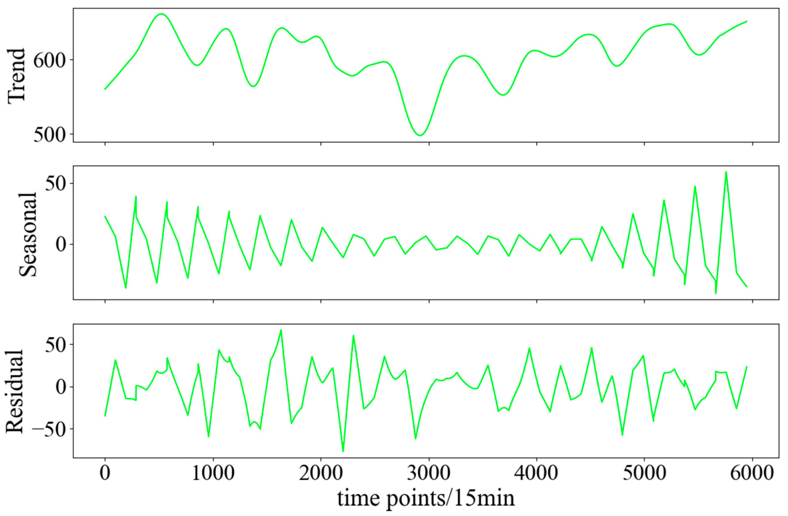
In this study, the seasonal period is set to 288, corresponding to a 3-day cycle (with each cycle consisting of 288 15-min time points), which captures the daily periodic fluctuations in the data. The seasonal window is set to 13, meaning that every 13 time points undergo seasonal smoothing, approximately equivalent to 3 h and 15 min, effectively smoothing short-term seasonal fluctuations. The trend window is not explicitly set. When the trend window is not specified, STL automatically adjusts the smoothing of the long-term trend based on the data’s characteristics. This adaptive trend smoothing method dynamically adjusts the smoothing level according to the long-term changes in the data.
The STL procedure proceeds as follows: the raw series is first subjected to a preliminary LOESS smoothing; the series is then partitioned by its seasonal period and each segment is smoothed separately to obtain the seasonal component; after the seasonal term is removed, the residual is smoothed again to extract the trend component. Nested inner and outer iterations iteratively update the trend and seasonal terms until stable convergence is achieved. The decomposition results are shown in Figure 3.
The raw series is first preprocessed with STL to strip out explicit trend and seasonal components; the resulting residuals are then fed into a hybrid model that couples VMD with Informer–BiGRU, enabling deeper exploitation of the series’ nonlinear and high-frequency features and thereby boosting forecasting performance.

2.2.2. VMD Decomposition Based on the Artificial Lemming Algorithm (ALA)

High energy-consuming power loads exhibit pronounced nonlinear behaviour. Although STL decomposition lowers the complexity of the residual relative to the raw data, the residual remains highly uncertain and therefore difficult to forecast. We thus further decompose the STL residual with VMD, generating components that display clear periodic characteristics. The hierarchical forecasting model obtained in this way shows definite advantages over a single-stage VMD approach, and experiments confirm that the hierarchical strategy delivers markedly higher prediction accuracy.
Variational mode decomposition (VMD) is a fully non-recursive, adaptive signal-decomposition technique that effectively eliminates the mode-mixing encountered in traditional modal-decomposition algorithms and is highly robust to noise, making it well suited to the load-decomposition requirements of high energy-consuming integrated-energy systems. Without sacrificing the original signal characteristics, VMD decomposes the input into several intrinsic mode functions (IMFs) with distinct centre frequencies; fundamentally, the procedure amounts to formulating and solving a constrained variational optimisation problem. The constrained variational model is expressed as follows:
m i n { u k } , { ω k } k = 1 K t u k ( t ) e j ω k t 2 2 s . t . k = 1 K u k ( t ) = f ( t )
In this formulation, f ( t ) is the original signal to be decomposed, u k ( t ) is the k t h intrinsic mode function (IMF), and ω k is the center frequency corresponding to u k ( t ) . The factor e j ω k t is a complex-exponential modulator, so u k ( t ) e j ω k t is the frequency-shifted version of the k t h mode. The operator t denotes temporal differentiation. The objective m i n { u k } , { ω k } k = 1 K t u k ( t ) e j ω k t 2 2 minimizes the total bandwidth across all modes, while the reconstruction constraint k = 1 K u k ( t ) = f ( t ) ensures that the IMFs collectively reproduce the original signal without loss.
To solve the variational problem, VMD introduces the Lagrange multiplier λ ( t ) and constructs an augmented Lagrangian, thereby transforming the constrained optimisation into an unconstrained one.
L ( { u k } , { ω k } , λ ) = α k = 1 K t u k ( t ) e j ω k t 2 2 + f ( t ) k = 1 K u k ( t ) 2 2 + λ ( t ) , f ( t ) k = 1 k u k ( t )
In variational mode decomposition, the penalty factor α limits the bandwidth convergence of each mode, whereas the number of modes K determines how many intrinsic mode functions can be extracted; selecting these parameters appropriately is crucial for obtaining a high-quality decomposition. An excessively large α can induce mode mixing and mask salient information, while an overly small α allows high-frequency noise to contaminate the components, leading to redundant modes. Likewise, setting K too high tends to overfit noise and increase signal complexity, whereas setting K too low leaves the useful signal insufficiently decomposed.
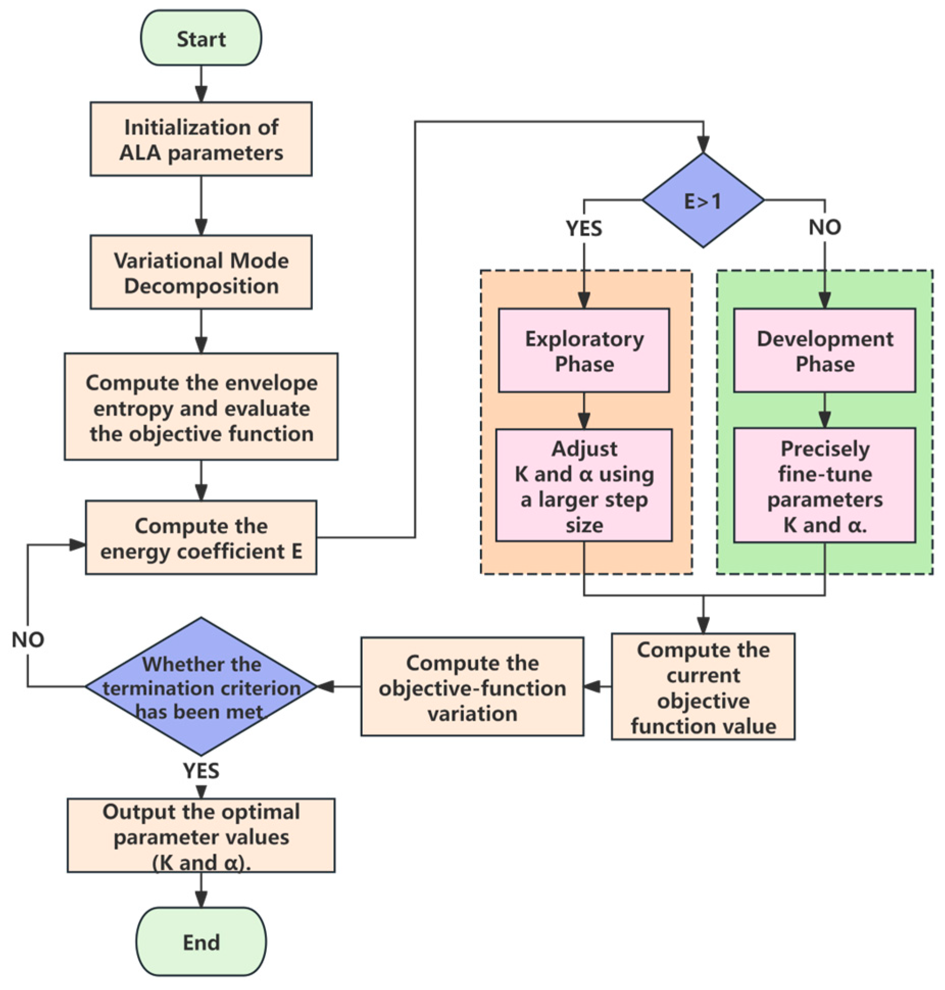
To eliminate the uncertainty inherent in empirically selecting parameters, this study employs the ALA algorithm to perform global collaborative optimization of the number of modes ( K ) and the quadratic penalty factor ( α ), thereby ensuring a rational choice of VMD decomposition parameters; envelope entropy [20] is adopted as the evaluation metric. Envelope entropy characterizes signal sparsity and is inversely related to periodicity: the clearer the signal’s periodicity, the lower its envelope-entropy value. Minimizing the mean envelope entropy is therefore set as the optimization objective; a lower mean value indicates that the corresponding IMF set possesses more pronounced periodic characteristics. Using the IMF set with the strongest periodicity as the model input simplifies multidimensional load modelling and enhances forecasting accuracy. Accordingly, by taking mean envelope entropy as the objective function and jointly adjusting the VMD mode number and quadratic penalty factor, the periodic information in the load sequence is extracted to the greatest extent, thereby improving decomposition quality. The procedure for calculating envelope entropy is as follows:
First, envelope extraction is performed via the Hilbert transform, which, for an input signal x t , is computed as follows:
E n v e l o p e ( t ) = H { x ( t ) }
The envelope entropy is then calculated as follows:
H ( u k ) = i = 1 N u k ( i ) l o g u k ( i )
where u k ( i ) denotes the envelope value of the k t h mode at the i t h time instant, and N is the length of the envelope sequence. The entropy value reflects the complexity of the signal envelope—the higher the entropy, the more complex the signal.
The objective function based on minimizing the mean envelope entropy is expressed as follows:
m i n K , α J ( K , α ) = 1 K k = 1 K H ( u k ) K m i n K K m a x α m i n α α m a x
where K and α denote the mode number and the quadratic penalty factor, respectively; K m i n and K m a x are the minimum and maximum allowable values of K ; and α m i n and α m a x are the minimum and maximum permissible values of α .
Given that high energy-consuming industrial loads typically display pronounced non-linearity, frequent disturbances, indistinct periodicity, and substantial noise in their time-series profiles, conventional optimisation algorithms often suffer from premature convergence and a limited search space when selecting decomposition parameters for such data, making it difficult to attain the global optimum. To overcome this challenge, we introduce a novel optimisation technique that mimics the collective behaviour of lemmings—the Artificial Lemming Algorithm (ALA).
The ALA algorithm can efficiently optimize multiple parameters in the VMD algorithm. Its unique mechanism, which simulates the collective behavior of lemming groups, provides outstanding global optimization ability and rapid local convergence in complex search spaces. Compared to the Grey Wolf Optimization (GWO) algorithm, ALA has stronger global optimization capability and the ability to avoid local optima, enabling a more comprehensive exploration of complex solution spaces. Compared to the White Whale Optimization (WOA) algorithm, ALA performs better in balancing global search and local convergence, effectively avoiding premature convergence while maintaining the depth of global search. Compared to Particle Swarm Optimization (PSO), ALA demonstrates stronger global exploration ability and faster convergence in high-dimensional complex problems, making it particularly suitable for complex optimization tasks. Therefore, using the ALA algorithm for VMD parameter optimization in this paper can significantly improve the precision and accuracy of the STL residual component VMD decomposition, providing a more reliable parameter optimization solution for deep feature extraction in high energy-consuming load sequences. These pronounced advantages have been thoroughly validated in ref. [21].
The detailed implementation procedure of the ALA is as follows:
Data preprocessing: The original power-load data are imported; missing values are imputed by interpolation, while outliers are removed and replaced with the median, thereby providing a clean input for subsequent variational mode decomposition (VMD).
Population initialization: The VMD mode number and quadratic penalty factor are mapped into a continuous vector space, allowing the ALA to optimise these parameters. Within the feasible domain, N lemmings are generated at random; in this study, the initial population size is set to N = 50 .
VMD decomposition: Each lemming’s current position serves as the parameter vector for VMD, which decomposes the residual component of the STL series into multiple intrinsic mode functions (IMFs).
Fitness evaluation: For the obtained IMFs, the envelope entropy of each mode is computed, followed by the calculation of the mean envelope entropy.
Energy-coefficient calculation: The energy coefficient E is the ALA’s decision variable; when E > 1 the algorithm performs a wide-range update, whereas E 1 triggers small-scale local exploitation.
Position update: In each generation, every lemming adjusts its position on the basis of its current location, the historical best solution, and the energy coefficient, preventing entrapment in local optima.
Convergence criterion: The algorithm terminates when the change in fitness values over ten consecutive generations falls below a predefined threshold; otherwise, position updates continue.
Output of optimal parameters: Once convergence is achieved, the optimal VMD parameters—those yielding the minimum mean envelope entropy—are exported. Using the optimal mode number and penalty factor, VMD is rerun, and the decomposed data are fed into the parallel forecasting framework for power-load prediction.
The detailed computational flow is illustrated in Figure 4:
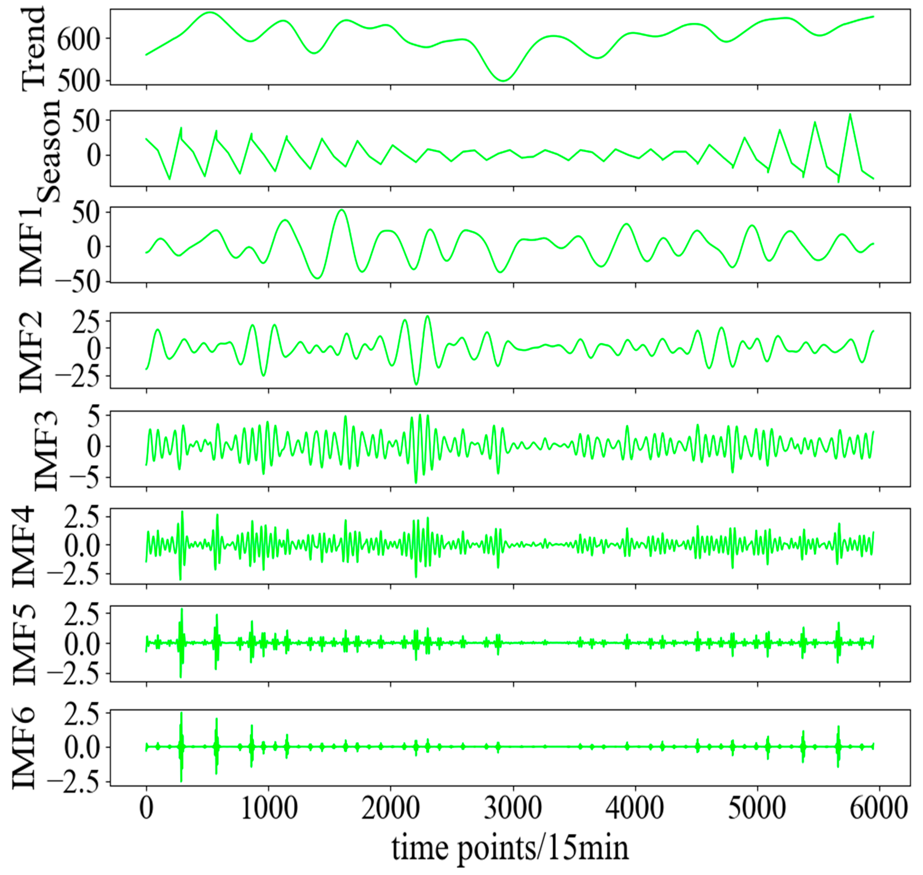
A second-stage decomposition is conducted with the optimal parameters obtained by the ALA, and the resulting components are presented in Figure 5.

3. Parallel Forecasting of High Energy-Consuming Loads Based on Informer and BiGRU

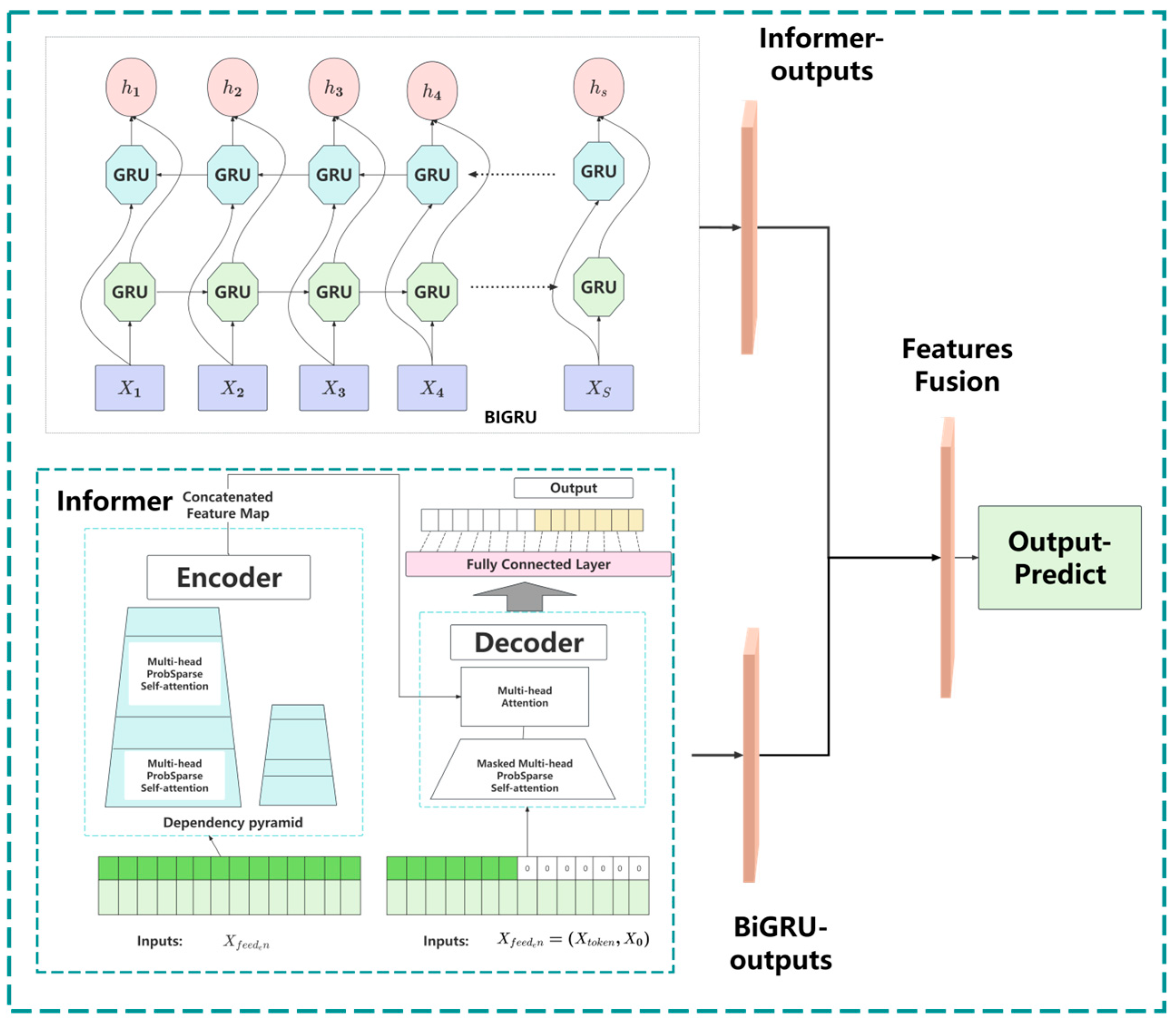
High energy-consuming load data are characterised by high dimensionality, complex fluctuations, and frequent dynamic changes; a single forecasting model generally fails to capture long-term trends and short-term abrupt variations with equal accuracy, resulting in sub-optimal performance. To address this limitation, we propose a parallel forecasting architecture that integrates an Informer with a bidirectional gated recurrent unit (BiGRU), as illustrated in Figure 6; two independent deep-learning branches operate concurrently to extract features from global long-range trends and local short-term fluctuations, respectively, thereby enabling accurate prediction of complex temporal load series.
The Informer, a Transformer architecture optimised specifically for long-sequence forecasting, introduces a probabilistic sparse self-attention mechanism that markedly reduces the computational burden faced by conventional Transformers when processing lengthy sequences, thereby substantially increasing model efficiency. Moreover, its generative decoder alleviates the information loss that can arise during long-horizon prediction and, together with global sparse self-attention and an adaptive-resolution mechanism, more effectively identifies and captures global features—such as long-term trends, seasonal fluctuations, and periodic variations—in load data, making the Informer particularly suitable for analysing and forecasting complex global patterns in long sequences.
In parallel, the BiGRU augments the standard GRU with a bidirectional information-processing mechanism, enabling it to learn features from sequence data in both past and future directions simultaneously. Compared with a unidirectional GRU, the BiGRU more effectively extracts local dynamic features and is more sensitive to short-term abrupt changes and local details in load data. Furthermore, its architecture is more compact than that of an LSTM, incurs lower computational overhead during training and inference, and converges more quickly, making it highly efficient for real-time forecasting scenarios. Consequently, the BiGRU excels at capturing the frequent short-term fluctuations, random disturbances, and sudden events characteristic of power-load series, markedly enhancing the model’s ability to predict local variation trends.
As depicted in Figure 7, once the Informer and BiGRU branches have independently extracted global and local features from the load data, a multilayer perceptron (MLP) is employed to fuse the resulting feature representations. This fusion strategy achieves deep integration and interaction of information, thereby further improving forecasting accuracy. Specifically, the MLP effectively combines the Informer’s global-trend information with the BiGRU’s local-fluctuation cues to generate synergistic features that enhance the model’s understanding and handling of complex temporal data. By means of this feature-fusion scheme, the model simultaneously capitalises on the Informer’s strength in modelling long-sequence global trends and the BiGRU’s aptitude for capturing short-term local variations, comprehensively boosting both the accuracy and robustness of forecasts for high energy-consuming loads.
Advantages of the parallel architecture: Its design mitigates the limitations that a single model may encounter when dealing with complex load data, thereby enhancing the overall stability and robustness of the forecasts. Because the Informer and BiGRU focus on global and local features of the data, respectively, the model can efficiently extract and integrate information across multiple temporal scales, making it particularly suitable for high energy-consuming industrial settings, data centres, and other power-load forecasting tasks. This parallel structure not only improves predictive accuracy but also augments the model’s adaptability, enabling outstanding performance in volatile industrial environments.
In summary, to address the multi-dimensionality, pronounced volatility, and dynamic variability of high energy-consuming load data, this study proposes a parallel forecasting model that integrates an Informer with a bidirectional gated recurrent unit (BiGRU). The Informer branch extracts global long-term trend features, whereas the BiGRU branch captures local short-term fluctuations; a multilayer perceptron (MLP) then fuses these representations, achieving deep integration of global and local information. Compared with conventional single-model approaches, the proposed parallel architecture concurrently accommodates trends and fluctuations across multiple time scales, markedly enhancing the accuracy, stability, and adaptability of forecasts for complex load data, and thus exhibits substantial application potential in high energy-consuming power-load prediction and related scenarios.

4. Construction of a Load Forecasting Framework for Typical Loads in High Energy-Consuming Industrial Parks Based on Multimodal Decomposition and Hybrid Neural Networks

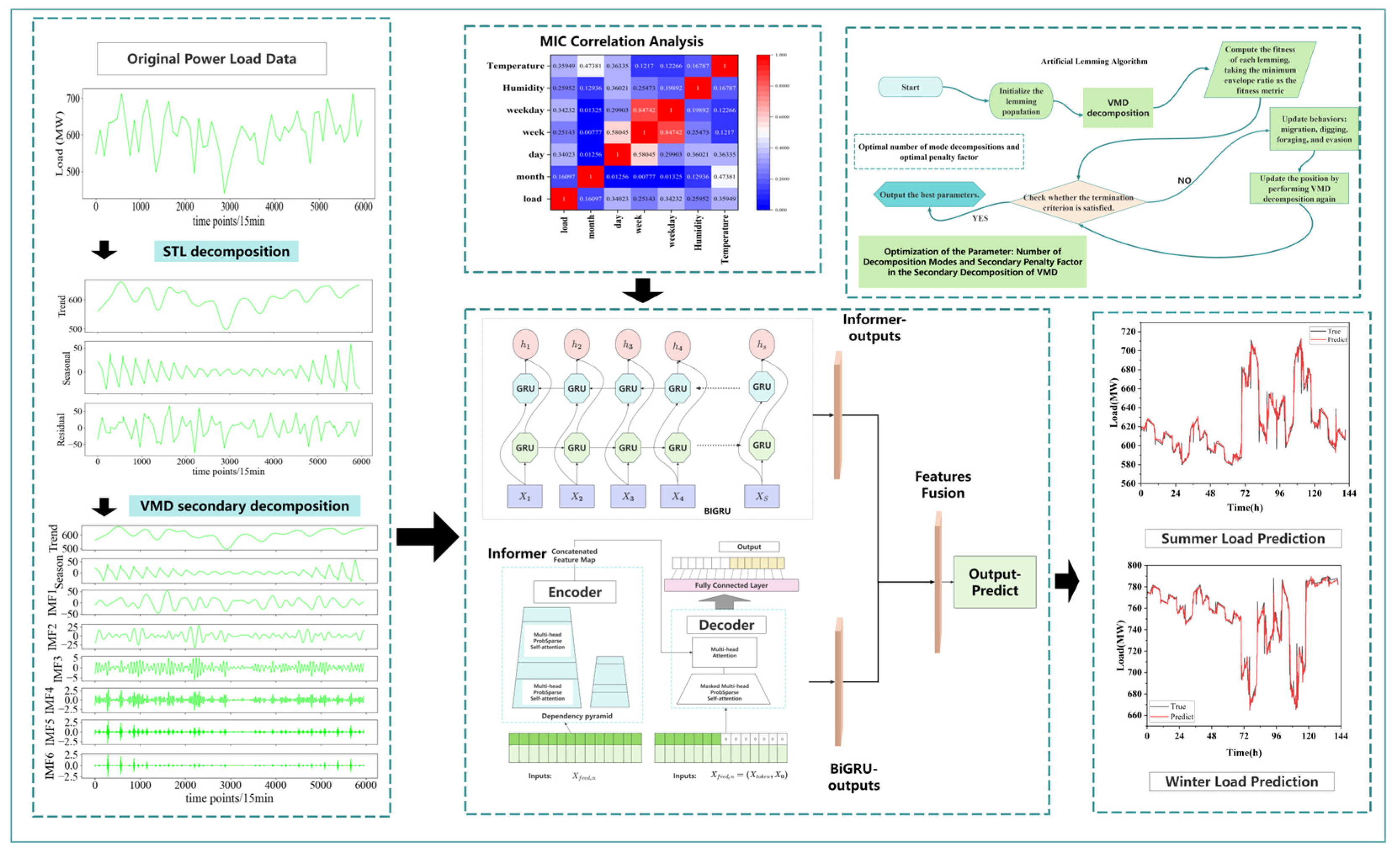
As illustrated in Figure 8, we propose a hierarchical modelling framework for forecasting high energy-consuming loads that fuses two deep-learning paradigms. The raw load data are first ingested and subjected to a two-stage hierarchical decomposition, followed by correlation analysis of the high energy-consuming load; the results are then processed through four parallel prediction-and-fusion modules to deliver highly accurate load forecasts. The detailed workflow is as follows:
First-stage hierarchical decomposition: The raw high energy-consuming load series is decomposed by seasonal-trend decomposition based on LOESS (STL), yielding three components: a trend component, a seasonal component, and a residual component.
Second-stage hierarchical decomposition: The residual component obtained from the STL decomposition is further analysed by variational mode decomposition (VMD); the optimal mode number and quadratic penalty factor are determined via the Artificial Lemming Algorithm (ALA), after which the residual is re-decomposed with VMD using these optimised parameters.
Correlation analysis: The maximal information coefficient (MIC) is applied to evaluate correlations and isolate the factors driving fluctuations in high energy-consuming loads; these explanatory variables are then supplied, alongside the load series itself, to the parallel forecasting framework.
Parallel forecasting: A BiGRU–Informer parallel architecture forecasts the load. The Informer branch captures global, long-term trends, whereas the BiGRU branch captures local, short-term fluctuations. Their respective feature representations are fused by a multilayer perceptron (MLP), enabling deep integration of information and producing the final high-precision forecast.

5. Numerical Example and Simulation Analysis

To verify the effectiveness of the proposed model, we investigated a representative high energy-consuming load in an industrial park located in northeastern China. A case study was conducted using 35,040 historical load observations and the corresponding meteorological data recorded from 16 April 2024 to 16 April 2025, with a sampling interval of 15 min. Because the region exhibits pronounced seasonal characteristics, separate load-forecasting experiments were performed for summer (June–July) and winter (December–January). The datasets for each season were partitioned into training, validation and test sets in an 8:1:1 ratio; the training set was used to fit the model, the validation set to tune hyper-parameters and select the best model, and the test set to assess final performance.

5.1. Data Preprocessing and Feature Input of High Energy-Consuming Loads

Outliers in the raw load data can severely compromise forecasting accuracy. Therefore, the interquartile range (IQR) method was used to detect and remove outliers, and the missing points were imputed with the mean of their adjacent samples.
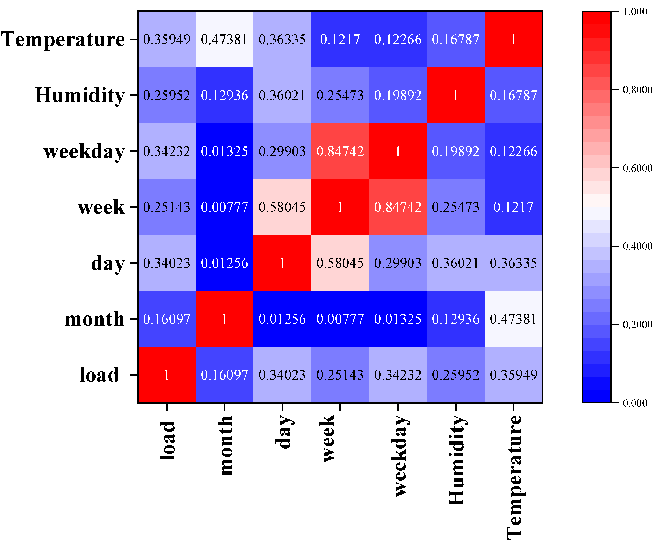
Potential factors correlated with the fluctuations of the high energy-consuming load were quantified using the maximal information coefficient (MIC); the detailed results are presented in Figure 9.
Because the selected high energy-consuming integrated energy system is located in northeastern China—where pronounced seasonal patterns lead to large temperature differences between winter and summer—its load is inevitably affected by ambient temperature. Figure 9 further confirms a strong association between the high energy-consuming load and temperature, with a correlation coefficient of ≈0.36. The same figure shows that the correlations between the load and both day type and weekday type are each ≈0.34. These results indicate that the load is also strongly influenced by these two factors, indirectly suggesting that it follows a distinct production rhythm. All three correlated factors are consistent with the real-world operating characteristics of the high energy-consuming integrated energy system. Consequently, temperature, day type and holiday type—identified by the MIC as the most influential factors—were incorporated as auxiliary features into the parallel load-forecasting architecture.

5.2. Prediction Experiments and Evaluation Metrics for High Energy-Consuming Loads

To rigorously assess the predictive performance of the proposed model for high energy-consuming loads, we carried out an ablation study in which the model was compared with VMD + Informer + BiGRU, VMD + BiGRU, BiGRU and GRU. For load decomposition, the hierarchical modelling strategy of the proposed approach was benchmarked against VMD, STL, CEEMD and EMD decompositions. Thus, the accuracy, applicability and effectiveness of the proposed method were evaluated from both the forecasting-model and decomposition-technique perspectives.
To rigorously evaluate the predictive capability of the proposed model, four performance metrics were employed: root mean square error (RMSE), mean absolute error (MAE), mean absolute percentage error (MAPE) and the coefficient of determination (R2). RMSE characterises the quadratic deviation between predicted and observed values; MAE quantifies the average absolute deviation of the predictions from the ground truth. MAPE emphasises the relative proportion of the error with respect to the actual value, thereby gauging the model’s scale-invariant accuracy across different magnitudes. R2 denotes the percentage of the total variance in the target variable that is explained by the model, serving as an indicator of goodness of fit. The mathematical expressions of these metrics are provided in Equations (8)–(11).
RMSE = 1 n i = 1 n ( y i y ^ i ) 2
MAE = 1 n i = 1 n | y i y ^ i |
MAPE = 1 n i = 1 n y i y ^ i y i × 100 %
R 2 = 1 i = 1 n ( y i y ^ i ) 2 i = 1 n ( y i y ¯ ) 2

5.3. Forecasting Results of High Energy-Consuming Loads

5.3.1. Ablation Experiments and Analysis

To evaluate the necessity and accuracy of each module within the proposed model, we carried out a comparative analysis against VMD + Informer + BiGRU, VMD + BiGRU and BiGRU. Because the chosen dataset exhibits pronounced seasonal characteristics—the average winter load is markedly higher than the summer load—we verified the superiority of the proposed model by separately examining the test-set results for the summer and winter seasons.
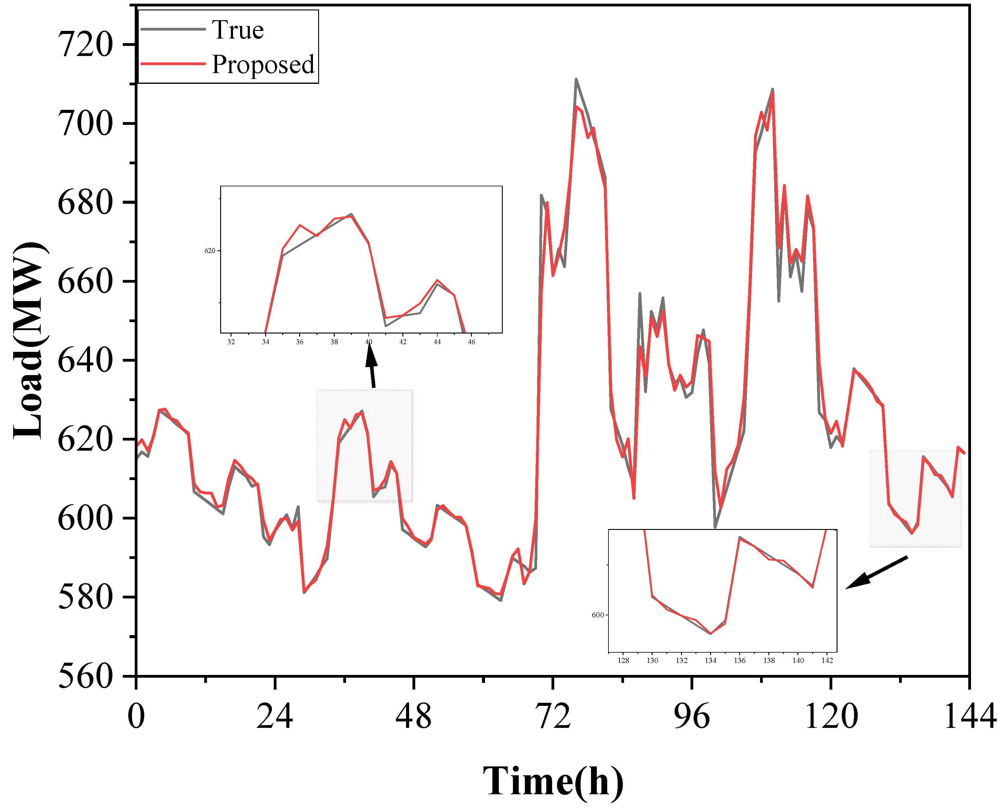
The comparative results for the summer season are illustrated in Figure 10. As can be seen, the proposed model achieves a good fit to the measured data. Moreover, the parallel forecasting framework not only overcomes the limited learning capacity of a single model but also markedly improves predictive accuracy. According to Table 1, the proposed framework yields RMSE, MAE and MAPE values of 13.4910, 2.4764 and 0.3934, respectively, on the summer test set—lower than those of any other ablation model—and achieves an R2 of 0.9873. This R2 is closer to unity than that of the competing models, underscoring the superiority of the proposed approach.
In the ablation study, VMD, Informer and STL were incrementally added to the baseline BiGRU. After incorporating VMD, RMSE, MAE and MAPE decreased by 23.46%, 19.65% and 23.23%, respectively, while R2 increased by 1.31%. VMD decomposition thus helps the model capture latent oscillatory or abrupt patterns in the load series, suppress noise and markedly improve forecasting accuracy and goodness of fit. Adding the Informer module further strengthens the modelling of long-range dependencies, enabling global features to be extracted from the denoised or decomposed signals—particularly for load series with long-period fluctuations or cross-day/week patterns. This optimisation reduces RMSE, MAE and MAPE by 20.51%, 21.23% and 21.51%, respectively, and raises R2 by 0.50%. To refine each modality, STL is employed to extract seasonal and trend components, thereby isolating periodic and slowly varying parts so that subsequent VMD can focus on high-frequency or non-stationary residues and Informer can capture global dependencies from a clearer multi-modal input. With STL included, RMSE, MAE and MAPE are further reduced by 32.01%, 14.16% and 13.90%, respectively, and R2 rises by 0.61%, providing additional evidence of the model’s effectiveness.
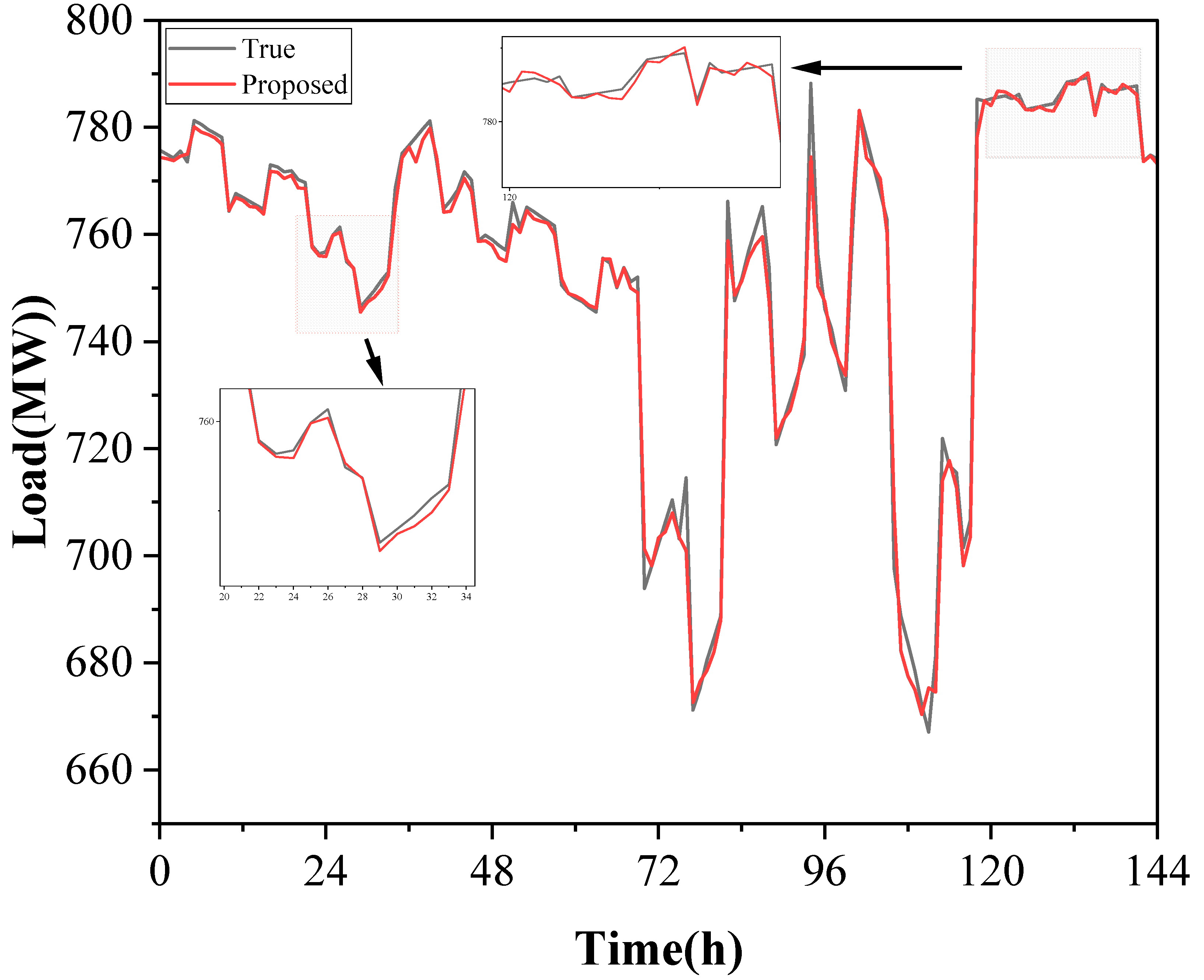
The comparative results for the winter season are presented in Figure 11, and the evaluation metrics are summarised in Table 2. After sequentially adding the VMD, Informer and STL modules to the baseline BiGRU, the corresponding performance indicators are reported as listed. Incorporating VMD into BiGRU reduces the first three metrics by 35.46%, 32.41% and 34.32%, respectively, while R2 increases by 1.81%. Adding the Informer module further lowers the first three metrics by 28.00%, 10.58% and 5.27%, and improves R2 by 0.28%. With the STL module included, the first three metrics decrease by an additional 29.87%, 24.36% and 24.13%, and R2 rises by 0.75%. This comparative winter analysis provides further evidence of the superiority of the proposed model in forecasting high energy-consuming electrical loads.
Analysis of the winter and summer forecasting results shows that the VMD, Informer and STL modules each serve a distinct yet complementary purpose in load prediction: VMD concentrates on noise removal, Informer captures long-range dependencies, and STL explicitly extracts seasonal and trend components. Their synergy markedly enhances the model’s generalisation ability and goodness of fit. By combining these decomposition and deep-learning modules in parallel or sequential configurations, the parallel forecasting framework overcomes the learning limitations of any single model and substantially improves the capture of complex load time-series patterns.

5.3.2. Analysis of the Impact of Different Modal Decomposition Methods on Prediction Performance

In this section, seasonal-trend decomposition using LOESS (STL), empirical mode decomposition (EMD), variational mode decomposition (VMD) and complete ensemble empirical mode decomposition (CEEMD) are employed as comparative methods, and the evaluation metrics for forecasting summer high energy-consuming loads are summarised in Table 3.
When applying VMD to decompose the residual component of STL, the minimum average envelope entropy is adopted as the objective function, and the adaptive learning algorithm (ALA) is used to tune the VMD parameters. The optimisation yields a decomposition mode number of 6 and a penalty factor of 962; therefore, these two parameters are set to 6 and 962, respectively, in the VMD decomposition carried out in this study.
Owing to the complex characteristics of the residual component produced by STL decomposition, accurately forecasting this component remains challenging. As indicated by the evaluation metrics in Table 3, the STL-only decomposition paired with the parallel forecasting model produces RMSE, MAE, MAPE and R2 values of 49.2103 MW, 4.8283 MW, 0.7673% and 0.9536, respectively, when forecasting the high energy-consuming load. None of the other STL-based combinations outperform the standalone parallel forecasting model, further corroborating the superiority of the parallel approach and the limitations of standalone STL decomposition.
Although empirical mode decomposition (EMD) can adaptively extract signal modes, it is prone to mode mixing, which prevents effective separation and modelling of high energy-consuming load characteristics. As shown in Table 3, coupling EMD alone with the parallel forecasting model yields a performance of RMSE = 57.2780 MW, MAE = 5.0476 MW, MAPE = 0.6588%, and R2 = 0.9460, which is markedly inferior to that of methods such as VMD or CEEMD. When combined with other modules, EMD also displays a considerable performance gap, indicating that its effectiveness for this task is limited.
Complete ensemble empirical mode decomposition (CEEMD) is an enhancement of EMD. During decomposition, it adds a pair of white-noise sequences with equal amplitude and opposite sign; the symmetric noise causes the noise effects in the two decompositions to cancel out when averaged, while the intrinsic modes that are useful to the signal are reinforced, thereby markedly mitigating mode mixing. Consequently, CEEMD achieves better results than EMD. As shown in Table 3, relative to EMD, CEEMD reduces the first three evaluation metrics for predicting high energy-consuming loads—RMSE, MAE and MAPE—by 42.99%, 12.17% and 17.71%, respectively, while increasing R2 by 2.45%. Table 3 also indicates that coupling CEEMD with the parallel forecasting model provides some improvement over combinations of CEEMD with other modules when predicting high energy-consuming loads; nevertheless, the overall predictive performance still leaves room for improvement.
When VMD is applied on its own, the minimum average envelope entropy is likewise adopted as the objective function to ensure effective decomposition of the complex high energy-consuming load; the resulting optimised parameters are [ K = 7 , α = 1120 ]. Coupling VMD with the parallel forecasting model yields RMSE, MAE, MAPE and R2 values of 19.8362 MW, 2.8849 MW, 0.4569% and 0.9813, respectively, for the high energy-consuming load forecast. These results indicate that VMD optimised with the minimum average envelope entropy effectively strips noise and multi-band components from the high energy-consuming load series, enabling the downstream model to focus on informative signals and thereby markedly improving forecast accuracy. Moreover, forecasts obtained by combining this VMD decomposition with other modules also outperform those based on alternative decomposition methods, further confirming its advantage.
To further enhance forecasting performance, an STL + VMD hierarchical modelling approach is proposed. Specifically, the raw power-load series is first decomposed using STL; because the resulting seasonal and trend components exhibit clear periodic behaviour whereas the residual component remains complex, VMD is subsequently applied to the residual, with the minimum average envelope entropy adopted as the objective function for this second-stage decomposition. According to Table 3, the hierarchical model achieves RMSE, MAE, MAPE and R2 values of 13.4910 MW, 2.4764 MW, 0.3934% and 0.9873, respectively. Relative to the strong baseline of VMD alone paired with the parallel model, the first three metrics are reduced by 32.01%, 14.16% and 13.90%, while R2 increases by 0.61%. These results further confirm that, by removing seasonal and trend components and focusing on residual details, the hierarchical STL + VMD framework substantially improves the accuracy of high energy-consuming load forecasts.
Likewise, Table 4 reports the evaluation metrics for winter high energy-consuming load forecasts produced by various decomposition-and-model combinations. According to Table 4, EMD yields the poorest performance relative to the other methods. When VMD optimised with the minimum average envelope entropy is employed, the four evaluation metrics are 17.2988 MW, 2.8880 MW, 0.3863% and 0.9822, indicating a satisfactory predictive capability. Building on this, replacing the stand-alone VMD with the hierarchical modelling framework further reduces the first three metrics by 29.87%, 24.36% and 24.13%, respectively, while raising R2 by 0.75%. These findings provide additional evidence of the superiority of the proposed model for high energy-consuming load forecasting.

5.3.3. STL, MIC, and ALA Methods’ Effectiveness Ablation Experiments

To verify the necessity of the STL, MIC, and ALA modules in the proposed model, models with each of these modules removed individually were constructed, and comparative experiments were conducted on both summer and winter test sets.
The evaluation metrics for the summer test set are shown in Table 5. The results of the four metrics indicate that removing any single module leads to a decrease in prediction accuracy. Compared with the model in which all three modules were removed, the proposed model achieves reductions of 39.33%, 40.5212%, and 38.7323% in RMSE, MAE, and MAPE, respectively, and an improvement of 1.87% in R2.
The evaluation metrics for the winter test set are presented in Table 6. When all three modules (STL, MIC, and ALA) are removed, RMSE, MAE, MAPE, and R2 are 17.3685 MW, 3.9597 MW, 0.4665%, and 0.9711, respectively. Compared with the proposed model, the first three metrics increase by 42.27%, 44.83%, and 37.17%, while R2 improves by 1.91%.
The prediction results from both the summer and winter test sets indicate that the STL, MIC, and ALA modules effectively enhance forecasting accuracy. Specifically, STL separates the seasonal and trend components, MIC efficiently eliminates redundant information that could interfere with the model, thereby optimizing the feature space, and the ALA algorithm effectively optimizes the parameters in VMD decomposition. The integration of these three modules significantly improves the overall prediction performance.

6. Conclusions

To fully mine the nonlinear characteristics embedded in high energy-consuming load data while simultaneously capturing both long-term trends and short-term patterns during forecasting, this study proposes a forecasting framework that couples an STL + VMD hierarchical decomposition with a BiGRU + Informer deep-learning ensemble. The VMD parameters are tuned via an adaptive learning algorithm that minimises the average envelope entropy; this design, tailored for noisy and strongly seasonal loads, allows the hierarchical decomposition to disentangle and refine the seasonal, trend and fine-grained frequency components of the series. The parallel forecasting framework then cooperatively learns short-term dynamic patterns and long-range dependencies. Using a representative load from an integrated high energy-consuming energy system in Northeast China as the case study, the empirical analysis yields the following key conclusions:
(1)
During VMD decomposition, the minimum average envelope entropy is adopted as the objective function, and an adaptive learning algorithm is employed to automatically optimise both the number of modes and the penalty factor, thereby ensuring a rational and stable separation of frequency-domain components in the high energy-consuming load series. A maximum information coefficient correlation analysis is then applied to identify features that are strongly related to load fluctuations, thus refining the input feature set for high energy-consuming load forecasting.
(2)
In the ablation experiments, starting from the baseline BiGRU module and sequentially introducing the VMD, Informer and STL components, RMSE, MAE and MAPE consistently decreased, while R2 steadily increased across both the summer and winter datasets, unequivocally demonstrating the indispensability of each module within the overall framework.
(3)
In the comparative experiments, the proposed STL + VMD hierarchical modelling strategy—unlike combinations based on other decomposition methods (such as STL, EMD, CEEMD or stand-alone VMD) and various deep-learning predictors—first explicitly extracts the seasonal and trend components, then applies multi-modal frequency decomposition to the residual, thereby capturing the fine-grained nonlinear characteristics of the load series more thoroughly. The parallel BiGRU–Informer ensemble simultaneously learns short-term dynamic patterns and long-range dependencies. Experiments show that, on both the summer and winter test sets, this framework reduces RMSE by an average of 30.94%, lowers MAE by 19.26%, decreases MAPE by 19.02%, and raises R2 by 0.68% relative to the stand-alone VMD + parallel-prediction architecture, thereby confirming the synergistic benefits of hierarchical modelling and parallel forecasting.
Although the proposed method has achieved good results in representative cases, there are still several limitations that warrant further exploration and improvement in future research. First, due to data availability constraints, this study did not account for the impact of renewable energy volatility on high energy-consuming load forecasts. This factor could have a significant impact on load during extreme weather conditions or unexpected events. Therefore, the model’s adaptability is limited when responding to abnormal or extreme situations. Second, the current study only employed two deep learning frameworks in parallel. Future research could explore incorporating other types of neural network architectures, such as Graph Neural Networks (GNN) or self-attention mechanisms (Transformers), to further enhance the model’s prediction accuracy and robustness. In addition, adopting multi-task learning (MTL) methods would be a promising direction, allowing the simultaneous optimization of multiple related tasks within the same framework to improve the model’s comprehensiveness and stability. Finally, to improve the model’s generalizability and practicality, future work should consider validating it in more complex and variable real-world environments, ensuring its ability to handle various uncertainties and environmental factors, thereby enhancing the reliability of the forecast results.
In summary, the STL + VMD hierarchical decomposition coupled with the parallel BiGRU + Informer forecasting framework proposed in this study fully exploits the nonlinear characteristics of high energy-consuming load data while accounting for both long-term trends and short-term dynamics, thereby markedly improving prediction accuracy. The findings can inform the operational planning and dispatching decisions of high energy-consuming integrated energy systems and offer practical guidance for future research that integrates multi-source data with more efficient models.

Author Contributions

Conceptualization, J.L. and Y.S.; methodology, J.L. and N.Z.; software, Y.S. and Y.C.; validation, J.L. and Y.S.; formal analysis, Y.S. and N.Z.; investigation, Y.C.; resources, Y.S.; data curation, J.L.; writing—original draft preparation, Y.S.; writing—review and editing, N.Z., J.L. and Y.S.; visualization, J.L. and N.Z.; supervision, J.L., Y.S. and Y.C.; project administration, J.L. and Y.S.; funding acquisition, J.L. All authors have read and agreed to the published version of the manuscript.

Funding

This research was funded by the Inner Mongolia Autonomous Region Science and Technology Breakthrough Project (2024KJTW0017) National Key Research and Development Plan Energy Storage and Smart Grid Technology Project (2024YFB2408400) and Inner Mongolia Natural Science Foundation under Grant (2025MS05012).

Institutional Review Board Statement

Not applicable.

Informed Consent Statement

Not applicable.

Data Availability Statement

The data presented in this study are available through request to the corresponding author.

Acknowledgments

During the preparation of this study, the authors used ChatGPT for correcting grammatical issues in the manuscript. The authors have reviewed and edited the output and take full responsibility for the content of this publication.

Conflicts of Interest

The authors declare no conflicts of interest.

References

  1. Chen, Z.; Wu, Z.; Wei, L.; Yang, L.; Yuan, B.; Zhou, M. Understanding the synergy of energy storage and renewables in decarbonization via random forest-based explainable AI. Appl. Energy 2025, 390, 125891. [Google Scholar] [CrossRef]
  2. Zhao, X.; Wang, Y.; Wang, B.; Liu, C.; Zhao, Y. Review of Market Implementation and Scheduling Models Considering the Flexibility Extraction of Differentiated Industrial Energy-Intensive Loads. Trans. China Electrotech. Soc. 2025, 40, 2043–2062, 2161. [Google Scholar]
  3. Chen, L.; Wang, C.; Wu, Z. Reinforcement Learning-Based Time of Use Pricing Design Toward Distributed Energy Integration in Low Carbon Power System. IEEE Trans. Netw. Sci. Eng. 2025, 12, 997–1010. [Google Scholar] [CrossRef]
  4. Zhou, X.; Qi, L.; Pan, N.; Hou, M.; Yang, J. Optimization method for load aggregation scheduling in industrial parks considering multiple interests and adjustable load classification. Energy 2025, 326, 135887. [Google Scholar] [CrossRef]
  5. Ma, S.; Wang, Q.; Nie, T.; Chen, Z.; Teng, Y. Collaborative optimization model of industrial high-energy consumption park under green and low-carbon transformation. Electron. Lett. 2024, 60, 13187. [Google Scholar] [CrossRef]
  6. Han, F.; Wang, X.; Qiao, J.; Shi, M.; Pu, T. Review on Artificial Intelligence Based Load Forecasting Research for the New-type Power System. Proc. Chin. Soc. Electr. Eng. 2023, 43, 8569–8591. [Google Scholar]
  7. Yang, T.; Zhao, L.; Wang, C. Review on Application of Artificial Intelligence in Power System and Integrated Energy System. Autom. Electr. Power Syst. 2019, 43, 2–14. [Google Scholar]
  8. Gao, S.; Li, F. Short-term wind speed forecasting based on CEEMD-SE-PSR-BP method. Acta Energiae Solaris Sin. 2025, 46, 415–422. [Google Scholar]
  9. Guo, W.; Liu, J.; Ma, J.; Lan, Z. Short-Term Power Load Forecasting Using Adaptive Mode Decomposition and Improved Least Squares Support Vector Machine. Energies 2025, 18, 2491. [Google Scholar] [CrossRef]
  10. Ye, J.; Cao, J.; Yang, L.; Luo, F. Ultra Short-term Load Forecasting of User Level Integrated Energy System Based on Variational Mode Decomposition and Multi-model Fusion. Power Syst. Technol. 2022, 46, 2610–2618. [Google Scholar]
  11. Huang, H.; Zhang, A.a. Load Forecasting of Integrated Energy System Based on Combination of Decomposition Algorithms and Meta-learning. Autom. Electr. Power Syst. 2024, 48, 151–160. [Google Scholar]
  12. Liu, W.; Hua, F.; Cui, Y.P.; Xu, Y.C.; Liu, H. An Optimized Power Load Forecasting Algorithm Based on VMD-SMA-LSTM. Energy Sci. Eng. 2025, 13, 3243–3253. [Google Scholar] [CrossRef]
  13. Xiao, W.; Mo, L.; Xu, Z.; Liu, C.; Zhang, Y. A hybrid electric load forecasting model based on decomposition considering fisher information. Appl. Energy 2024, 364, 123149. [Google Scholar] [CrossRef]
  14. Wang, H.; Yan, J.; Zhang, J.; Liu, S.; Liu, Y.; Han, S.; Qu, T. Short-term integrated forecasting method for wind power, solar power, and system load based on variable attention mechanism and multi-task learning. Energy 2024, 304, 132188. [Google Scholar] [CrossRef]
  15. Li, X.; Wang, Z.; Yang, C.; Bozkurt, A. An advanced framework for net electricity consumption prediction: Incorporating novel machine learning models and optimization algorithms. Energy 2024, 296, 131259. [Google Scholar] [CrossRef]
  16. Cao, Z.; Wang, J.; Xia, Y. Combined electricity load-forecasting system based on weighted fuzzy time series and deep neural networks. Eng. Appl. Artif. Intell. 2024, 132, 108375. [Google Scholar] [CrossRef]
  17. Wang, C.; Wu, Z.; Wei, L.; Yang, L.; Zhang, Y.; Yuan, B.; Zhou, M. Evaluating the externality value of distributed photovoltaics: Industry-specific investment decisions under diverse pricing schemes. Renew. Energy 2025, 247, 122986. [Google Scholar] [CrossRef]
  18. You, W.; Guo, D.; Wu, Y.; Li, W. Multiple Load Forecasting of Integrated Energy System Based on Sequential-Parallel Hybrid Ensemble Learning. Energies 2023, 16, 3268. [Google Scholar] [CrossRef]
  19. Gong, J.; Qu, Z.; Zhu, Z.; Xu, H. Parallel TimesNet-BiLSTM model for ultra-short-term photovoltaic power forecasting using STL decomposition and auto-tuning. Energy 2025, 320, 135286. [Google Scholar] [CrossRef]
  20. Gu, L.; Wang, J.; Liu, J. A combined system based on data preprocessing and optimization algorithm for electricity load forecasting. Comput. Ind. Eng. 2024, 191, 110114. [Google Scholar] [CrossRef]
  21. Xiao, Y.; Cui, H.; Abu Khurma, R.; Castillo, P.A. Artificial lemming algorithm: A novel bionic meta-heuristic technique for solving real-world engineering optimization problems. Artif. Intell. Rev. 2025, 58, 84. [Google Scholar] [CrossRef]
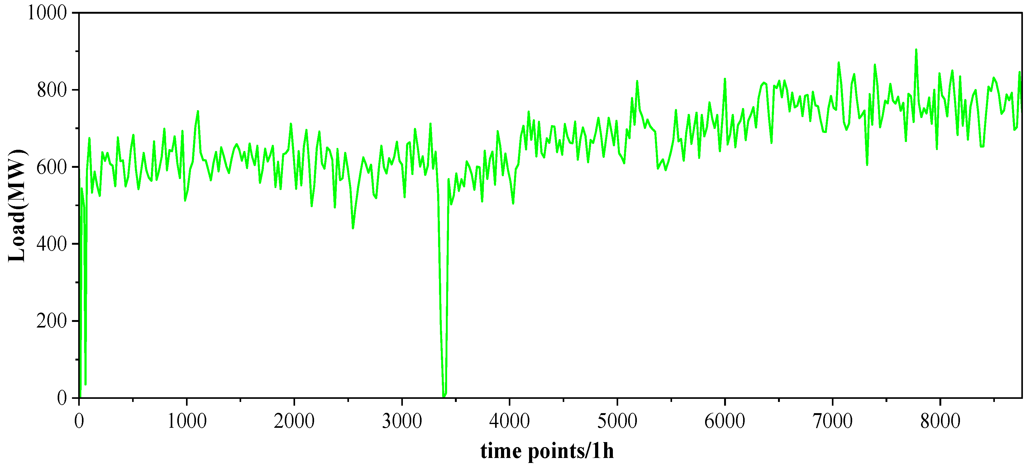
Figure 1. One-Year Load Data from a Northeast China High Energy-Consuming Park.
Applsci 15 09578 g001
Figure 2. Summer Load of High Energy-Consuming Industry.
Applsci 15 09578 g002
Figure 3. STL Decomposition Plot of Summer Load in High Energy-Consuming Industry.
Applsci 15 09578 g003
Figure 4. Flowchart of the Artificial Lemming Algorithm (ALA).
Applsci 15 09578 g004
Figure 5. VMD Decomposition Plot of the Residual Component from STL.
Applsci 15 09578 g005
Figure 6. Parallel Forecasting Architecture Diagram.
Applsci 15 09578 g006
Figure 7. Flowchart of Parallel Fusion Strategy.
Applsci 15 09578 g007
Figure 8. Overall Framework Diagram of High Energy-Consuming Load Forecasting.
Applsci 15 09578 g008
Figure 9. Correlation Analysis Results Plot.
Applsci 15 09578 g009
Figure 10. Comparison of Proposed Forecast Model vs. Actual Load for Summer.
Applsci 15 09578 g010
Figure 11. Comparison of Proposed Forecast Model vs. Actual Load for Winter.
Applsci 15 09578 g011
Table 1. Evaluation Metrics for Summer Ablation Experiments.
Forecasting ModelRMSE
(MW)
MAE
(MW)
MAPE (%)R2
Proposed13.49102.47640.39340.9873
VMD + Informer + BIGRU19.83622.88490.45690.9813
VMD + BIGRU24.95293.66250.58210.9764
BIGRU32.60014.55810.75820.9638
Table 2. Evaluation Metrics for Winter Ablation Experiments.
Forecasting ModelRMSE (MW)MAE (MW)MAPE (%)R2
Proposed10.02762.18440.29310.9896
VMD + Informer + BIGRU14.29882.88800.38630.9822
VMD + BIGRU19.85783.22980.40780.9795
BIGRU30.76964.77820.62090.9621
Table 3. Evaluation Metrics of Forecasting Using Different Decomposition Methods in Summer.
Decomposition MethodForecasting
Model
Evaluation Metrics
RMSE
(MW)
MAE
(MW)
MAPE
(%)
R2
ProposedProposed13.49102.47640.39340.9873
GRU26.65003.55560.56300.9748
BIGRU19.78212.77680.43780.9803
Informer38.94993.72520.58790.9632
VMDProposed19.83622.88490.45690.9813
GRU26.65003.95560.66300.9748
BIGRU24.95293.66250.58210.9764
Informer41.33764.55710.72630.9610
STLProposed49.21034.82830.76730.9536
GRU95.21757.93501.18030.9101
BIGRU61.82206.24451.00140.9417
Informer116.72629.34501.35930.8898
CEEMDProposed32.65424.43340.70670.9692
GRU62.39685.00290.87920.9412
BIGRU44.21104.70520.76120.9583
Informer87.09307.34481.28260.9178
EMDProposed57.27805.04760.85880.9460
GRU88.98556.91490.81260.9160
BIGRU85.04186.34200.68260.9197
Informer102.52727.19560.97640.9032
Table 4. Evaluation Metrics of Forecasting Using Different Decomposition Methods in Winter.
Decomposition MethodForecasting
Model
Evaluation Metrics
RMSE
(MW)
MAE
(MW)
MAPE
(%)
R2
ProposedProposed10.02762.18440.29310.9896
GRU22.08703.61710.48400.9773
BIGRU16.85952.74260.36910.9826
Informer33.97303.71290.50150.9650
VMDProposed14.29882.88800.38630.9822
GRU26.13513.64660.43050.9731
BIGRU19.85783.22980.40780.9795
Informer35.27964.36510.58780.9637
STLProposed48.46314.95100.66630.9502
GRU72.20946.83420.82230.9258
BIGRU57.07865.46870.70310.9413
Informer100.67427.17470.96240.8965
CEEMDProposed34.89013.92590.53070.9641
GRU56.10025.41580.69580.9423
BIGRU48.30114.81230.64620.9503
Informer70.21646.63170.85090.9278
EMDProposed54.09754.89220.65530.9444
GRU74.80176.27710.87040.9231
BIGRU69.38556.04970.81660.9287
Informer79.37107.79640.95010.9084
Table 5. Evaluation Metrics of Forecasting for Method Effectiveness in Summer.
Forecasting ModelRMSE
(MW)
MAE
(MW)
MAPE (%)R2
Proposed13.49102.47640.39340.9873
Without STL19.83622.88490.45690.9813
Without STL + ALA21.63213.86410.52320.9732
Without STL + ALA + MIC22.23684.16350.64210.9692
Table 6. Evaluation Metrics of Forecasting for Method Effectiveness in Winter.
Forecasting ModelRMSE (MW)MAE (MW)MAPE (%)R2
Proposed10.02762.18440.29310.9896
VMD + Informer + BIGRU14.29882.88800.38630.9822
VMD + BIGRU19.85783.22980.40780.9795
BIGRU30.76964.77820.62090.9621
Disclaimer/Publisher’s Note: The statements, opinions and data contained in all publications are solely those of the individual author(s) and contributor(s) and not of MDPI and/or the editor(s). MDPI and/or the editor(s) disclaim responsibility for any injury to people or property resulting from any ideas, methods, instructions or products referred to in the content.