Prediction Models for Nitrogen Content in Metal at Various Stages of the Basic Oxygen Furnace Steelmaking Process

Abstract

Controlling dissolved nitrogen is critical to meeting increasingly stringent steel quality targets, yet the variable kinetics of gas absorption and removal across production stages complicate real-time decision-making. Leveraging a total of 291 metal samples, the research applied ordinary least squares (OLS) regression, enhanced by cointegration diagnostics, to develop four stage-specific models covering pig iron after desulfurization, crude steel in the basic oxygen furnace (BOF) before tapping, steel at the beginning and end of secondary metallurgy processing. Predictor selection combined thermodynamic reasoning and correlation analysis to produce prediction equations that passed heteroscedasticity, normality, autocorrelation, collinearity, and graphical residual distribution tests. The k-fold cross-validation method was also used to evaluate models’ performance. The models achieved an adequate accuracy of 77.23–83.46% for their respective stages. These findings demonstrate that statistically robust and physically interpretable regressions can capture the complex interplay between kinetics and the various processes that govern nitrogen pick-up and removal. All data are from U. S. Steel Košice, Slovakia; thus, the models capture specific setup, raw materials, and production practices. After adaptation within the knowledge transfer, implementing these models in process control systems could enable proactive parameter optimization and reduce laboratory delays, ultimately minimizing excessive nitrogenation in finished steel.

1. Introduction

In recent years, controlling the amount of nitrogen in the steelmaking process has become increasingly important. Controlling nitrogen content is important because high nitrogen content in metal has an overall adverse effect on the properties of the steel produced [1,2]. An exception is nitrogen in austenitic stainless steel, where the presence of nitrogen is desirable [3,4,5,6,7,8]. Increased nitrogen content leads to a deterioration in deep drawability and resistance to ageing, reduces the degree of recrystallization, and also impairs the mechanical properties of steel, which include formability and strength [9,10,11]. The increased presence of nitrogen in general steel also negatively affects the weldability of steel [12,13] (over 0.4 wt.% Nitrogen), as well as the electrical parameters [14]. In general, the nitrogen content of steel produced in a basic oxygen furnace (BOF) ranges from 20 to 60 ppm. Steel can contain nitrogen in an unbound form or as a chemical compound, such as a nitride [15]. A large number of factors influence the nitrogen content in steel, and their interaction during the steelmaking process determines the final nitrogen value. The solubility of gases in molten metals is generally very low, which leads to the consideration of gases in metals as infinitely diluted solutions [16]. The process of nitrogen dissolving in molten metal is dictated by Equation (1), and the Gibbs free energy associated with this process is expressed by Equation (2) [15,16,17,18,19]. An explanation of all symbols listed in this paper can be found in the “List of symbols” at the end of the article.

½ N_2(g) = [N]

(1)

ΔG° = −3590 − 23.89 T [J.mol⁻¹]

(2)

The equilibrium constant of Equation (1) has the form of Equation (3) [16,20].

$$K_N={\displaystyle \frac{a_N}{{\left(p_{N_2}\right)}^{\frac{1}{2}}}}={\displaystyle \frac{f_N\left[\%N\right]}{\sqrt{p_{N_2}}}}\left[P{a}^{-1/2}\right]$$

(3)

Given that nitrogen in molten metal is a diluted solution, it can be assumed that f_N = 1 [21,22]. Equation (1) being endothermic, it can be deduced that the solubility of nitrogen in the molten state increases with rising temperature. The solubility of nitrogen in liquid metal is found to be significantly dependent on gas pressure, temperature, and also on the metal itself, whose chemical composition undergoes substantial changes during the smelting process. Equation (4) expresses the relationship between the quantity of elemental nitrogen dissolved in metal and the pressure at which it is held above the molten metal at a constant temperature, which is known as Sievert’s law [16,17,20,23,24].

$$\left[\%N\right]=K_N\cdot {\left(p_{N_2}\right)}^{{\displaystyle \frac{1}{2}}}$$

(4)

In the event that the dissolution of gases in metals occurs in strict accordance with Sievert’s law, this serves as an indication that the gas is present in the liquid metal in its elemental form. However, in reality, the dependence of gas solubility on pressure is often more complex. This observation indicates that gas may not be present in metals exclusively in atomic form. Relevant results according to Sieverts’ law are also only achieved at lower gas pressures above the surface of the liquid metal [16,25]. The temperature-dependent amount of dissolved elemental gas in molten metal can be expressed at constant pressure via the following Equation (5) [26].

$$\left[\%N\right]=C·e^{{\displaystyle \frac{-\Delta H}{2kT}}}$$

(5)

According to the established relationship, it can be determined that the concentration of dissolved nitrogen in molten metal is directly proportional to the equilibrium constant KN, as depicted in Equation (1). Van’t Hoff’s reaction isobar demonstrates that the equilibrium constant is a function of temperature as showed in Equation (6).

$${\displaystyle \frac{dln{K}_N}{dT}}={\displaystyle \frac{\Delta H}{R{T}^2}}$$

(6)

A significant increase in the solubility of nitrogen in iron is observed at a temperature of 907 °C. As the data demonstrate, with an increase in temperature, the solubility of nitrogen in γ-Fe decreases, which is related to the formation of Fe₄N and Fe₂N nitrides according to Equations (7) and (8) [27].

2 N + 8 Fe ↔ 2 Fe₄N

(7)

N + 2 Fe ↔ Fe₂N

(8)

The courses of Equations (7) and (8) are exothermic, with values that exceed the negative value of the heat of dissolution of nitrogen in iron. Therefore, as demonstrated in Equation (5), it can be concluded that the solubility of nitrogen in γ-Fe decreases with rising temperature.

In addition to iron, nitrogen in steel also reacts with other elements dissolved in the melt. This process gives rise to the formation of various chemical compounds, the existence of which depends on several factors. These include the chemical composition of the steel, the sequence of the steelmaking process, the temperature or pressure within the system, and the subsequent heat treatment of the steel. Figure 1a illustrates the impact of specific elements on the solubility of nitrogen in molten iron [28,29].

The presence of nitrogen in molten metal solutions has a significant influence, primarily due to the amount of carbon present. In this regard, the status of carbon (Figure 1b) is determined by the fact that its atoms occupy analogous positions to iron atoms when the crystal lattice forms. At the same time, carbon reacts with oxygen to form CO bubbles, which carry nitrogen atoms as they travel through the metal towards the surface [30].

In the event that the steel under consideration contains multiple dissolved elements, the solubility of nitrogen in the poly-component system can be expressed based on the transformed Equation (3) into the following Equation (9), which can be modified to form Equation (10).

$$a_{\left[N\right]}=f_{\left[N\right]}\cdot {\left[N\right]}_{steel}=K_N\cdot \sqrt{p_{N_2}}$$

(9)

$$log{\left[N\right]}_{steel}=log{K}_N+0.5log.p_{N_2}-log{f}_{\left[N\right]}$$

(10)

The application of Sieverts law allows for the determination of the dependence of solubility on the heat, pressure, and chemical composition of steel, as expressed by Equation (11). The activity coefficient of nitrogen, f_[N], is expressed as a function of elemental content, $e_N^E$, according to the following Equation (12), while the activity coefficient of nitrogen in the multicomponent system (Fe–N...E) is determined by the Wagner equation according to Equation (13).

$$log{\left[N\right]}_{steel}=-375T-1.154+0.5log.p_{N_2}-log{f}_{\left[N\right]}$$

(11)

$$log{f}_N^E=e_N^E.\left[\%E\right]$$

(12)

$$f_N^{Fe\dots E}=f_N^{*}.f_N^C.f_N^D\dots f_N^E$$

(13)

The actual nitrogen content in the metal melt is determined by the dissolution rate of nitrogen in the melt $\left(v_{N_{diss}}\right)$ and the removal rate of nitrogen from the melt $\left(v_{N_{rmvl}}\right)$. The temporal variation in the nitrogen content [N] of the melt, as a function of the blowing time (τ), is calculated by Equation (14).

$${\displaystyle \frac{d\left[N\right]}{d\tau }}=v_{N_{diss}}-v_{N_{rmvl}}$$

(14)

The dissolution of nitrogen into molten metal can be described by the sequence of the following individual steps [29,31,32]: (1) transfer of nitrogen molecules from the gas volume to the phase interface; (2) adsorption of nitrogen molecules on the interfacial layer; (3) Reaction at the phase interface; (4) desorption of nitrogen atoms from the phase interface; (5) diffusion of nitrogen atoms from the gas-melt phase interface by melt flow into its volume.

Desorption followed by diffusion of nitrogen atoms into the metal volume probably has the greatest effect on the dissolution rate of nitrogen in liquid metal, as these are the slowest processes in the sequence of steps described above. As the rate of dissolution is determined by the slowest action, it is possible to formulate Equation (15) for the kinetics of nitrogen dissolution in molten metal [17].

$$v_{N_{diss}}={\displaystyle \frac{D}{\delta }}\cdot S\cdot \left({\left[N\right]}_{srfc}-{\left[N\right]}_{vol}\right) \left[mol.s^{-1}\right]$$

(15)

The dissolution rate of nitrogen in molten metal is defined by Equations (16) and (17), as stated in the literature [17]. Equation (16) is used for the calculation at low concentrations of surfactants such as sulfur and oxygen, while Equation (17) is applied to find the dissolution kinetics of nitrogen at high concentrations of these elements.

$${\displaystyle \frac{d{C}_{\left[N\right]}}{dt}}={\displaystyle \frac{A}{V}}\cdot k\cdot \left(C_{\left[N\right]eq.}-C_{\left[N\right]}\right)$$

(16)

$${\displaystyle \frac{d{C}_{\left[N\right]}}{dt}}={\displaystyle \frac{A}{V}}\cdot k\cdot \left(C_{\left[N\right]eq.}^2-C_{\left[N\right]}^2\right)$$

(17)

The determination of the kinetics of nitrogen dissolution in metal can be achieved through the utilization of Equation (18), which is dependent on the composition of the metal solution, its concentration, and the temperature [33].

$$k={\displaystyle \frac{D}{\delta }}\cdot S=\beta \cdot S$$

(18)

Figure 2a,b shows a graphical representation of the nitrogen dissolution rate constant β in Fe–C and Fe–O alloys as a function of temperature and the concentration of the given element.

Improper control of nitrogen content during steel production can lead to critical quality issues that significantly compromise the mechanical properties, surface quality, and overall performance of steel products. These issues occur at various stages of production. One of the most significant quality issues associated with high nitrogen content is the formation of gas bubbles and porosity in steel. Nitrogen has limited solubility in molten steel, and its solubility decreases dramatically as temperature drops during solidification. Nitrogen bubbles form within the steel if nitrogen exceeds the solubility limit [34,35]. Research indicates that chromium increases nitrogen solubility most significantly, followed by manganese and molybdenum, while nickel decreases solubility. This compositional sensitivity requires careful alloy design to control nitrogen effects [34]. The formation of these bubbles follows Sieverts’ law, which describes the dependence of gas concentration on pressure [35]. The porosity formation is particularly problematic in welding operations [36]. Steel can become brittle when exposed to high nitrogen concentrations, particularly when combined with other interstitial elements [37]. Improper nitrogen control can increase susceptibility to cold cracking, particularly in high-strength steels. The interstitial nitrogen atoms create stress concentrations that can initiate and propagate cracks [38]. Excessive nitrogen pickup reduces the steel’s ability to deform plastically, leading to premature failure under load. This is particularly critical in structural applications, where ductility is essential for safety reasons [39].

Linear regression effectively predicts metallurgical outputs (production, temperature, strength, corrosion, nitrogen content) when relationships are approximately linear. With proper variable selection, data cleaning, and validation, it achieves up to 8% measurement accuracy [40]. Its advantages include simple implementation, high interpretability, and fast calculations. Combined with kinetic/thermodynamic models, it provides fundamental process understanding [41]. Random Forest algorithms consistently achieve 88–92% success across parameters, offering noise resistance and variable importance identification [42,43]. Support Vector Regression (SVR) and Extreme Learning Machine (ELM) excel in specific applications, with ELM providing extremely fast training [44]. Neural networks and Deep Learning demonstrate the highest accuracy (R² = 0.79–0.92) for various parameters [42,45,46], forming promising real-time solutions for comprehensive nitrogen content prediction in steelmaking processes.

The models presented in the available scientific literature focus on predicting the nitrogen content in metal in only one specific phase of BOF steel production. The novel aspect of this study is that it provides a comprehensive perspective on predicting the nitrogen content in metal throughout the entire BOF production cycle. This approach to the matter has not yet been published in the available studies.

The main aim was to develop predictive models of nitrogen content in liquid pig iron and liquid steel. The proposed approach to the model and the scope of research applied to the entire steel production cycle have not yet been developed in such a comprehensive form and published in professional literature. Models were created to predict the nitrogen content of metal at four production stages, namely, the nitrogen content of pig iron after desulphurization, the nitrogen content of crude steel before tapping from basic oxygen furnace (BOF) to the ladle, the nitrogen content of steel at the beginning of secondary metallurgy processing, and the nitrogen content of steel at the end of secondary metallurgy processing. This facilitates the monitoring of the development of nitrogen content in metal at each crucial production stage of a specific heat. This provides a tool for appropriate corrective intervention in the production process and its optimization to achieve the required quality parameters.

It is notable that all data originate from U. S. Steel Košice, Slovakia; as such, the models under consideration are representative of specific technological settings, raw materials, and production practices. Following adaptation within the knowledge transfer, implementation of these models in process control systems has the potential to enable proactive parameter optimization and reduce laboratory delays, minimizing excessive nitrogenation of finished steel.

2. Materials and Methods

The production process of the material used to generate the data for this article can be summarized as follows. Pig iron produced in a blast furnace was pretreated (desulfurized) using a vertical refractory lance (Scandinavian lance) with a CaO–Mg-based mixture for desulfurization. This mixture was blown into the pig iron using nitrogen as the carrier gas. The pig iron was then charged into a top-blown basic oxygen furnace (BOF/LD process), where a water-cooled oxygen lance was used to blow high-purity oxygen at supersonic velocity onto the surface of the metal to oxidize the impurities. The BOF’s capacity was 170 tons. After approximately 17 min, the crude steel was tapped into a steel ladle. During tapping from the BOF, the steel in the ladle was deoxidized by adding aluminum and alloyed by adding ferroalloys. The steel chemical composition and thermal composition were also finished and stirred in the ladle by blowing/bubbling argon through a porous plug at the bottom. The chemical composition of the steel was finally refined, and the temperature was finally optimized by blowing/bubbling argon through a porous refractory block located at the bottom of the ladle. The analyzed heats were not vacuum-treated in the RH vacuum degasser. At the end of secondary metallurgy, the steel was prepared for casting on a continuous casting machine. The flow charts (Figure A1a–d) that illustrate the overall research framework and model implementation within given phases can be found in Appendix A.

A total of 291 metal samples from 76 heats were collected from 17 May 2025 to 22 May 2025 and analyzed for their nitrogen content. The sampling design aimed to obtain samples from all four production phases within a single heat. This made it possible to monitor the amount of nitrogen in a given heat and how it varied throughout the production process. A collection of 76 samples (standard “lollypop-shaped” samples) was obtained from pig iron after desulfurization from the ladle, 68 samples were obtained from crude steel before tapping from BOF, 75 samples were obtained from molten steel in the ladle at the beginning of secondary metallurgy, and 72 samples were obtained from molten steel in the ladle at the end of secondary metallurgy. The reason why it was not possible to obtain exactly 76 samples from each phase was most likely due to a failure in sampling, in which it was not possible to adequately and reliably evaluate the nitrogen content in the sample itself.

The samples taken consisted of two grades of steel. The first was a structural steel grade with a manganese content above 0.80% and a guaranteed Al content with the following prescribed composition: 0.07–0.21% C; 0.8–1.6% Mn; 0.03–0.6% Si; min 0.02% Al; max. 0.025% P; max. 0.020% S. The second grade was deep-drawing Al-killed steel with the following prescribed composition: 0.02–0.1% C; 0.1–0.55% Mn; max. 0.08% Si; 0.02–0.07% Al; 0.01–0.07% P; max. 0.020% S; 0.004–0.0075% Nb.

The samples were evaluated for nitrogen content in pig iron and steel at the certified Quantometric laboratory of U. S. Steel Košice (Labortest, s.r.o.) by using a combustion analyzer ELTRA ON 900 (ELTRA GmbH, Haan, Germany) that determines nitrogen using a thermal conductivity detection method (based on ASTM E-1019 standard [47]). The equipment is calibrated by the manufacturer and checked once a year by the manufacturer’s service technician. Every four hours, a laboratory technician checks the device by using a sample standard. The analyzer has a measurement range of 0.0001–0.03% N with an error range of ±0.1 ppm or ±1% of nitrogen content. Two measurements, main and control, are evaluated.

The nitrogen content of the metal was determined using heat and sample identification numbers. These data were synchronized with relevant databases containing records of the metal’s chemical composition, temperature, weight, and other parameters attributable to that stage of processing. The synchronized parameter database was initially compiled in Microsoft Excel 365 with the Lumivero XLSTAT 2019 statistical add-in. Subsequently, the correlation matrix, generated using STATISTICA 7.0 from StatSoft Inc. (Tulsa, OK, USA), enabled the determination of the order of factors affecting the final nitrogen content at a given stage of production. The data file was processed using Gretl 2025a (build 2025-03-20), a powerful and sophisticated statistical tool. The k-fold cross-validation was performed using the open-source program Orange Data Mining 3.39.0 from the Bioinformatics Lab at the University of Ljubljana, Slovenia.

Determining the factors and assessing their impact on the amount of nitrogen in metal is a key attribute in optimizing technological and operational measures aimed at minimizing or preventing over-nitrogenation of the final steel. It is crucial to identify and quantify the influence of individual factors on the nitrogen content in metal to effectively address the issue of predicting its quantity during the production and processing stages of steelmaking. A correlation matrix was created that included all analyzed factors, which made it possible to determine the quantitative dependence in which changes in one variable lead to changes in another.

This dependence is expressed by a function called a regression function. Depending on its shape, the regression function can indicate a positive or negative correlation. A positive correlation occurs when the regression function is increasing, and a negative correlation occurs when the regression function is decreasing. Each indicator was subjected to classical and modern regression analysis, while elements of cointegration analysis of non-stationary variables were also applied [48].

The existence of linear correlation dependence in a two-dimensional statistical set is indicated by the presence of a covariance in Equation (19).

$$k=S_{xy}={\displaystyle \frac{1}{n}}\cdot {\displaystyle \sum }_{i=1}^n\left(x_i-\overline{x}\right)\cdot \left(y_i-\overline{y}\right)$$

(19)

where (x_i, y_i) are individual pairs of observations, $\overline{x}$ and $\overline{y}$are the corresponding arithmetic means. The covariance depends on the choice of scale for the values of random variables ξ and η. Therefore, Pearson’s correlation coefficient is used to measure the degree of linear correlation [49,50]. The correlation coefficient of a statistical set ranges within the closed interval 〈−1,1〉. In absolute terms, the value approaches 1 as the linear correlation between the variables ξ and η increases. The calculation of the correlation coefficient of a two-dimensional basic set is performed in accordance with the following Equation (20) [51].

$$\rho \left(\xi ,\eta \right)={\displaystyle \frac{cov\left(\xi ,\eta \right)}{\sqrt{D\left(\xi \right)\cdot D\left(\eta \right)}}}$$

(20)

The correlation coefficient R measures the strength of statistical dependence between two quantitative variables. Unlike regression, correlation analysis does not express a cause-and-effect relationship Y = f(X). Variable Y does not depend on variable X, but the two random variables X and Y change together. Regression analysis assumes that variable Y is random and variable X is fixed. The term correlation coefficient most often refers to Pearson’s correlation coefficient in Equation (21) [52].

$$R_{xy}={\displaystyle \frac{\sum x_i{y}_i-n\overline{x}\overline{y}}{\left(n-1\right)s_x{s}_y}}$$

(21)

As demonstrated in Equation (21), it is feasible to identify the order of relevance of the factors that exert the most significant influence on the amount of nitrogen in the metal within a specific phase of steel production in a closed cycle. The objective of this study was to identify the most significant factors for each phase that was analyzed.

The interpretation of the correlation coefficient R depends on the context and nature of the data. A value of 0.8 is very low for verifying a physical law, but very high for the social sciences [53,54]. Jacob Cohen developed a simplified instrument for the interpretation of correlation coefficients in research [55], as illustrated in

Table 1. Cohan’s interpretation of correlation coefficients [55].

Correlation coefficient	0–0.1	0.1–0.3	0.3–0.5	0.5–0.7	0.7–0.9	0.9–1
Correlation interpretation	trivial, very small	little, low	moderate	big, high	very big, very high	perfect, clear

.

The R² value (22) is referred to as the coefficient of determination, which quantifies the proportion of common variability between two variables. The R² value achieved is contingent upon the nature of the data being processed. The interpretation of the coefficient of determination values achieved is significantly influenced by the nature of the analyzed data.

$$R_{xy}^2=1-{\displaystyle \frac{s_{y|x}^2}{s_y^2}} \mathrm{or}{R}_{xy}^2=-{\displaystyle \frac{s_{x|y}^2}{s_x^2}}$$

(22)

Non-stationarity is a property of time series or datasets in which the statistical properties (e.g., mean, variance) are shown to change over time. Econometrics is characterized by the utilization of non-stationary datasets, a principle that aligns with the methodologies employed in metallurgy [56,57]. In the field of economic sciences, it has been established that coefficient of determination values above R² = 0.15 are not achieved [58]. Non-stationarity is also observed in metallurgical data, particularly in processes where conditions vary over time, such as temperatures during melting, cooling, or changes in chemical composition during metal processing [59].

The combination of modern linear regression analysis and cointegration analysis enables the design, analysis, and verification of predictive models that can be applied in operating conditions. Non-stationary variables are a characteristic of metallurgy. When such time-dependent variables are used, there is a risk of spurious regression. This occurs when there is no cointegration effect between non-stationary variables, i.e., no long-term, stable relationship. If spurious regression were not detected, this would negatively impact the identification of factors, the interpretation of results, and the application of the model in real technological practice. In this study, cointegration analysis was employed to validate the model derived from modern linear regression analysis.

The Ordinary Least Squares (OLS) method was used for data processing. Compared to other estimation techniques, the OLS method provides optimal estimates even for small samples of observations, and the algorithm for calculating these estimates is relatively simple [60,61]. Furthermore, this method forms the basis of a wide range of more sophisticated estimation tests and procedures.

For statistical processing purposes, the following general model was proposed for calculating the predicted amount of nitrogen in metal at individual stages of steel production (23).

$$N_n=z_0+z_1·Z_1+z_2·Z_2+\cdots +z_n·Z_n$$

(23)

Adequate coefficients were calculated for the analyzed factors influencing the amount of nitrogen present in metal during the various stages of steel production. The corresponding standard error, t-ratio, and p-value were also calculated for each coefficient. The t-ratio parameter expresses the value of the standard deviation [62,63] and assesses whether two groups (dependent and independent) differ statistically from each other [64]. The p-value is a random variable based on the measured values of the monitored quantity. It expresses the probability of obtaining a value at least as extreme as the one actually observed, assuming the null hypothesis is true. It ranges [0, 1] [65].

In statistical hypothesis testing, the null hypothesis formally evaluates specific aspects of the statistical behavior of datasets. This evaluation is considered valid if the actual behavior of the datasets contradicts the assumption. Consequently, the null hypothesis can be accepted or rejected [66]. The proposed models were analyzed using several verification methods, such as the heteroscedasticity test, normality test, autocorrelation test, collinearity test, and graphical examination of residual distribution. To confirm the accuracy of the conclusions of the modern regression analysis, an econometric cointegration analysis was also performed.

The estimation of reliable performance was accomplished through the utilization of k-fold cross-validation. This statistical technique is used to evaluate the performance of statistical models. It operates on the principle of dividing a dataset into k equal parts (folds). In this study, the setting k = 10 (10-fold cross-validation) was employed due to the smaller dataset. This configuration engenders reduced bias, with 90% of the data being utilized for training in each iteration. In an analogous manner, when k = 10, a sufficient number of iterations are performed to obtain stable results, which also represents computational efficiency.

The following were used to determine the accuracy of the prediction models: Mean Absolute Error (MAE), which expresses the average absolute deviation of the actual values from the estimated (or predicted) values. MAE is determined using Equation (24).

$$MAE={\displaystyle \frac{1}{n}}{\displaystyle \sum }_{t=1}^n\left|e_t\right|$$

(24)

The Mean Percentage Error (MPE), which expresses the degree of distortion, was also applied to determine the accuracy of the model. Equation (25) can be used to calculate whether the model underestimates or overestimates reality.

$$MPE={\displaystyle \frac{1}{n}}{\displaystyle \sum }_{t=1}^n{\displaystyle \frac{e_t}{y_t}}\cdot 100\left[\%\right]$$

(25)

Mean Absolute Percentage Error (MAPE), according to Equation (26), was used to express the average size of forecast errors as a percentage of the actual measured values over the entire forecasting period [67].

$$MAPE={\displaystyle \frac{1}{n}}{\displaystyle \sum }_{t=1}^n{\displaystyle \frac{\left|e_t\right|}{y_t}}\cdot 100\left[\%\right]$$

(26)

The accuracy of the entire model is determined according to Equation (27).

Model accuracy: N_stage = 100 − MAPE [%]

(27)

3. Results

Determining the factors and assessing their impact on the nitrogen content of metal is key to optimizing technological and operational measures to minimize or prevent excessive nitrogenation of the final steel. The identification and quantification of the influence of individual factors on the nitrogen content in metal is imperative for the effective prediction of its quantity during the production and particular steelmaking processing stages. Through the synthesis of correlation analysis findings, physical and empirical evidence, the most significant agents were identified, thereby establishing a foundation for subsequent, more intricate statistical procedures. This study utilized a comprehensive analytical approach encompassing classical and modern regression analysis, complemented by elements of cointegration analysis of non-stationary variables employed in econometric time series analyses.

3.1. Parameters Affecting the Amount of Nitrogen in Molten Desulfurized Pig Iron

As shown in

Table 2. Ranking of factors affecting the nitrogen content in desulphurized pig iron.

Rank	Coefficient	Factor	Correlation Coefficient R	Coefficient of Determination R2
1.	a1	Amount of sulfur removed [%]	0.2226	0.0495
2.	a2	Amount of nitrogen added as a carrier gas [l]	0.1379	0.0190
3.	a3	Weight of pig iron after desulfurization [kg]	0.1123	0.0126
4.	a4	Amount of desulphurization mixture [kg]	0.0965	0.0093
5.	a5	Temp. difference before and after desulfurization [°C]	0.0964	0.0093

, the following factors have been identified as the most significant in determining the amount of nitrogen present in desulphurized pig iron: the results of the regression analysis were obtained using a correlation matrix. As demonstrated in Table 2, the correlation indices could be interpreted as low to trivial according to Table 1. However, it should be noted that these are non-stationary integrated variables, where high correlation coefficients are not achieved even though these parameters have a significant effect on the dependent variable, which in this case is nitrogen.

Figure 3 shows a graphical representation of the effect of the amount of nitrogen added as a carrier gas for the desulphurization mixture on the amount of sulfur removed and the resulting nitrogen content of the pig iron. Figure 4a,b illustrates the impact of certain parameters listed in Table 2 on the final nitrogen content in metal during the desulphurization phase of pig iron processing. As demonstrated in Figure 4a, an increase in the amount of sulfur removed results in an increase in the amount of nitrogen present in the pig iron. Similarly, Figure 4b illustrates that an increase in the amount of nitrogen blown results in an increase in the amount of nitrogen dissolved in the pig iron A more thorough examination of the results is presented in Section 4.1.

Table 3. Conditions for statistical testing of nitrogen presence in pig iron before desulphurization.

Entry Requirement	Value
Significance level, α	0.05 *
Number of observations, n	76
Number of parameters, m	5

* Unless otherwise stated.

shows the conditions for statistical testing of nitrogen presence in pig iron before the desulphurization process.

Table 4. Results of a modern regression analysis of the factors influencing the nitrogen content in metal during the desulfurization phase of pig iron.

Coefficient	Value	Standard Error	t-Ratio	p-Value
a0	0.000105058	0.0081269	0.0129	0.98972
a1	0.0220528	0.00959012	2.2995	0.02446
a2	2.5678 × 10−8	2.69278 × 10−8	0.9536	0.34357
a3	2.50746 × 10−8	5.74314 × 10−8	0.4366	0.66374
a4	−2.35159 × 10−6	1.38981 × 10−6	−1.6920	0.09509
a5	4.96884 × 10−6	1.0213 × 10−5	0.4865	0.62812

Where: a₀ constant/intercept, a₁–a₅ coefficients of variables (from Table 2).

and

Table 5. Results of individual tests using modern regression analysis to identify the factors influencing nitrogen content in metal during the desulphurization phase of pig iron production.

Parameter	Value
Mean value of the dependent variable	0.003958
Sum of squared residuals	0.000036
R2—Coefficient of Multiple Determination	0.097373
F(5, 70)—F-test	1.510277
Standard deviation of the dependent variable	0.000730
Durbin–Watson test	1.641496

show the results of modern regression analysis for the individual factors (variables) listed in Table 2.

3.2. Parameters Affecting the Amount of Nitrogen in Molten Crude Steel Before Tapping from BOF

Table 6. Ranking of factors affecting the nitrogen content in crude steel before tapping from BOF.

Rank	Coefficient	Factor	Correlation Coefficient R	Coefficient of Determination R2
1.	b1	Oxygen reblow time [s]	0.4291	0.1842
2.	b2	Manganese content in crude steel [%]	−0.3017	0.0910
3.	b3	Phosphorus content in crude steel [%]	−0.2339	0.0547
4.	b4	Carbon content in crude steel [%]	−0.2055	0.0422
5.	b5	Briquettes [kg]	−0.1594	0.0254
6.	b6	Temperature of tapping steel [°C]	0.1457	0.0212
7.	b7	Oxygen blowing time [s]	−0.1314	0.0173

lists the most significant factors affecting the amount of nitrogen in crude steel before its tapping from BOF.

Based on Cohen’s distribution, the correlation coefficients can be interpreted as ranging from small to medium. However, it is important to note the non-stationary nature of the data from integrated systems, and that achieving medium correlation coefficient values with operational data is a great success.

Figure 5 shows the effect of the levels of phosphorus and manganese in crude steel on the final nitrogen content in crude steel before its tapping from BOF. Figure 6a–d illustrates the impact of certain parameters listed in Table 6 on the final nitrogen content in crude steel produced in BOF prior to tapping into the ladle. As illustrated in Figure 6a, an increase in the amount of manganese in crude steel is accompanied by a decrease in the amount of nitrogen dissolved in crude steel. In a similar manner, an increase in phosphorus (Figure 6b) and carbon (Figure 6c) results in a decrease in the amount of nitrogen dissolved in crude steel. Conversely, an increase in the temperature of crude steel (Figure 6d) has been shown to result in an increase in the amount of nitrogen dissolved in the crude steel. Further analysis of the results is provided in Section 4.2.

The conditions for the statistical testing of nitrogen presence in crude steel prior to tapping from the BOF are provided in

Table 7. Conditions for statistical testing of nitrogen presence in steel before tapping from BOF.

Entry Requirement	Value
Significance level, α	0.05 *
Number of observations, n	63
Number of parameters, m	7

* Unless otherwise stated.

.

Table 8. Results of a modern regression analysis (OLS) of the factors influencing the nitrogen content in crude steel prior to tapping from BOF.

Coefficient	Value	Standard Error	t-Ratio	p-Value
b0	−0.0137962	0.0113016	−1.2207	0.22740
b1	7.06124 × 10−6	2.94964 × 10−6	2.3939	0.02011
b2	−0.000306035	0.00286768	−0.1067	0.91540
b3	−0.0469186	0.0353764	−1.3263	0.19023
b4	−0.00499063	0.00482186	−1.0350	0.30520
b5	−3.44051 × 10−8	7.63705 × 10−8	−0.4505	0.65412
b6	1.04457 × 10−5	6.87455 × 10−6	1.5195	0.13437
b7	−3.96352 × 10−7	4.22613 × 10−7	−0.9379	0.35242

Where: b₀ constant/intercept, b₁–b₇ coefficients of variables (from Table 6).

and

Table 9. Results of individual tests using modern regression analysis to identify the factors influencing nitrogen content in crude steel before its tapping from BOF.

Parameter	Value
Mean value of the dependent variable	0.002002
Sum of squared residuals	0.000017
R2—Coefficient of Multiple Determination	0.292051
F(7, 55)—F-test	2.326593
Standard deviation of the dependent variable	0.000614
Durbin–Watson test	2.000830

present the findings of modern regression analysis for the individual factors (variables) enumerated in Table 6. It can be observed that correct results were achieved using the OLS method.

3.3. Parameters Affecting the Amount of Nitrogen in Molten Steel at the Beginning of Secondary Metallurgy

Table 10. Ranking of factors affecting the nitrogen content in steel at the beginning of secondary metallurgy.

Rank	Coefficient	Factor	Correlation Coefficient R	Coefficient of Determination R2
1.	c1	Tapping angle [°]	−0.4470	0.1998
2.	c2	Silicon in molten steel prior to argon bubbling [%]	0.3711	0.1377
3.	c3	Total aluminum prior to argon bubbling [%]	−0.2749	0.0756
4.	c4	Carbon in molten steel prior to argon bubbling [%]	0.2285	0.0522
5.	c5	Manganese in molten steel prior to argon bubbling [%]	0.2251	0.0507
6.	c6	Tapping time [s]	0.2203	0.0485
7.	c7	Added aluminum blocks [kg]	0.2040	0.0416

lists the strongest factors influencing the amount of nitrogen in steel at the beginning of secondary metallurgy (SM).

Based on Table 1, the results in Table 10 can be interpreted as indicating small to medium levels of dependency. However, higher correlation coefficient values can be observed when compared to the results in Table 6. Figure 7, Figure 8 and Figure 9 illustrate the impact of certain parameters from Table 10 on the nitrogen content of molten steel at the beginning of the SM processing. It is evident from Figure 9a,b that an increase in the amount of carbon and manganese in the molten steel prior to argon bubbling results in an increase in the amount of nitrogen dissolved in the molten steel. A more detailed analysis of the results can be found in Section 4.3.

Table 11. Conditions for statistical testing of nitrogen presence in steel at the beginning of secondary metallurgy.

Entry Requirement	Value
Significance level, α	0.05 *
Number of observations, n	75
Number of parameters, m	7

* Unless otherwise stated.

shows the conditions for statistical testing of nitrogen presence in steel at the beginning of secondary metallurgy processing.

Table 12. Results of a modern regression analysis (OLS) of the factors influencing the nitrogen content in steel at the beginning of the SM processing.

Coefficient	Value	Standard Error	t-Ratio	p-Value
c0	0.00982567	0.00228811	4.2942	0.00006
c1	−7.89409 × 10−5	1.89305 × 10−5	−4.1700	0.00009
c2	0.00368566	0.00143795	2.5631	0.01262
c3	−0.00987549	0.00757363	−1.3039	0.19672
c4	0.00442257	0.00595744	0.7424	0.46046
c5	−0.00140863	0.000838822	−1.6793	0.09775
c6	6.15271 × 10−7	1.35425 × 10−6	0.4543	0.65106
c7	6.28702 × 10−6	3.14335 × 10−6	2.0001	0.04955

Where: c₀ constant/intercept, c₁–c₇ coefficients of variables (from Table 10).

and

Table 13. Results of individual tests using modern regression analysis to identify the factors influencing the final nitrogen content in steel at the beginning of the SM processing.

Parameter	Value
Mean value of the dependent variable	0.003160
Sum of squared residuals	0.000035
R2—Coefficient of Multiple Determination	0.402680
F(7, 67)—F-test	6.452518
Standard deviation of the dependent variable	0.000888
Durbin–Watson test	1.872243

present the outcomes of a modern regression analysis of the individual factors (variables) listed in Table 10. The tables demonstrate that the correct results were obtained using the ordinary least squares method (OLS).

3.4. Parameters Affecting the Amount of Nitrogen in Molten Steel at the End of Secondary Metallurgy

Table 14. Ranking of factors affecting the nitrogen content in steel at the end of secondary metallurgy (SM).

Rank	Coefficient	Factor	Correlation Coefficient R	Coefficient of Determination R2
1.	d1	Steel temperature at the end of SM [°C]	−0.2768	0.0766
2.	d2	Final carbon in molten steel [%]	0.2268	0.0514
3.	d3	Addition of FeMn aff. during SM [%]	0.2056	0.0423
4.	d4	Final manganese in molten steel [%]	0.1930	0.0372

shows the most significant factors that influence the nitrogen content of steel at the end of the secondary metallurgy processing.

According to Cohen’s distribution, the correlation coefficient values from Table 14 are low. Figure 10a–d illustrates the factors from Table 14 that influence the final nitrogen content in steel at the end of the secondary metallurgy processing. It can be seen in Figure 10a that, as the temperature of the steel increases at the end of SM, the amount of dissolved nitrogen in the molten steel decreases. Figure 10b shows that, as the final amount of carbon in the molten steel increases, the amount of nitrogen in the molten steel also increases. Adding FeMn aff. ferroalloy (Figure 10c) increases the amount of nitrogen in the liquid steel, and increasing the amount of manganese in the steel (Figure 10d) increases the amount of nitrogen in the steel at the end of SM. Further analysis of the results is provided in Section 4.4.

The conditions for statistical testing of nitrogen presence in steel at the end of secondary metallurgy processing are shown in

Table 15. Conditions for statistical testing of nitrogen presence in steel at the end of secondary metallurgy.

Entry Requirement	Value
Significance level, α	0.05 *
Number of observations, n	72
Number of parameters, m	4

* Unless otherwise stated.

.

Table 16. Results of a modern regression analysis (OLS) of the factors influencing the nitrogen content in steel at the end of the SM processing.

Coefficient	Value	Standard Error	t-Ratio	p-Value
d0	0.0257714	0.0241686	1.066	0.2902
d1	−1.45992 × 10−5	1.52140 × 10−5	−0.9596	0.3408
d2	0.0126950	0.00645446	1.967	0.0534
d3	3.08438 × 10−6	1.63553 × 10−6	1.886	0.0637
d4	−0.00153525	0.000911391	−1.685	0.0968

Where: d₀ constant/intercept, d₁–d₄ coefficients of variables (from Table 14).

and

Table 17. Results of individual tests using modern regression analysis to identify the factors influencing the final nitrogen content in steel at the end of the SM processing.

Parameter	Value
Mean value of the dependent variable	0.003270
Sum of squared residuals	0.000033
R2—Coefficient of Multiple Determination	0.241736
F(4, 67)—F-test	2.682089
Standard deviation of the dependent variable	0.000790
Durbin–Watson test	2.029951

show the results of a regression analysis of the individual factors (variables) listed in Table 14. The tables confirm that the correct results were obtained using the OLS method.

4. Discussion

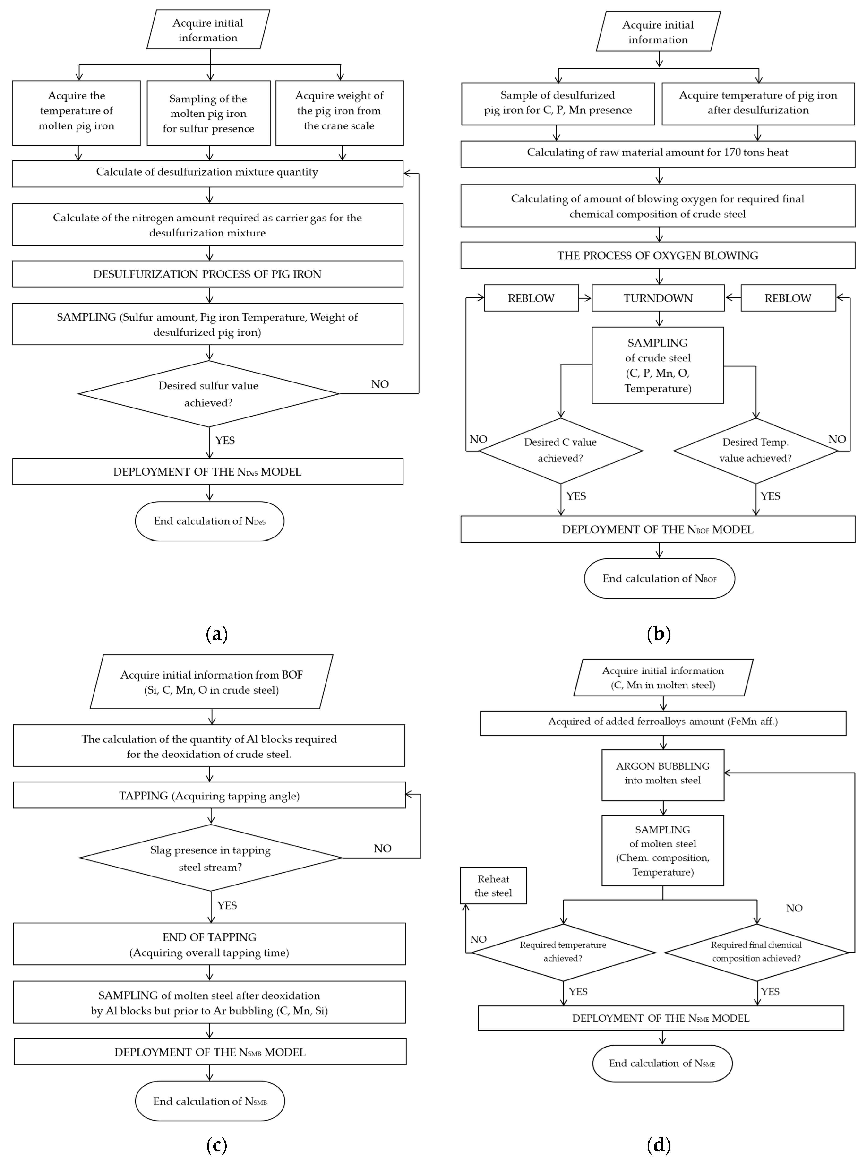
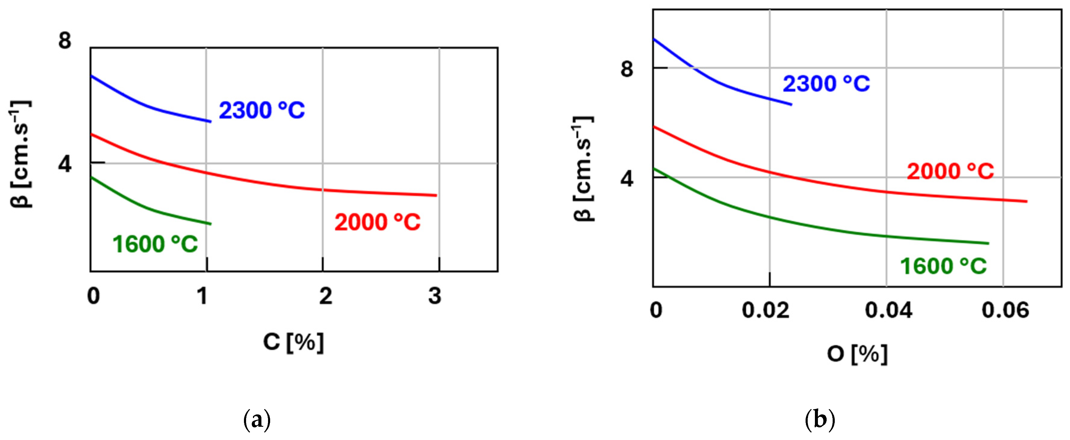
4.1. Model for Predicting Nitrogen Content in Molten Desulphurized Pig Iron

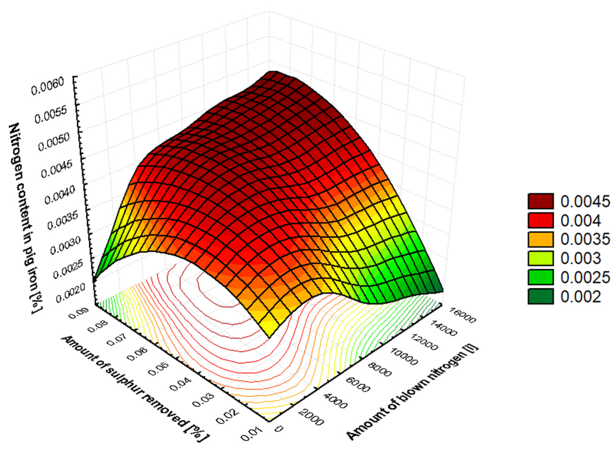
Section 3.1 contains Table 2, which shows the order of influence of the significant factors that cause metal saturation by nitrogen during the desulfurization phase of pig iron. The amount of nitrogen in pig iron after desulfurization is most influenced by the amount of sulfur removed from the pig iron. Sulphur is a strong surface-active element in pig iron, occupying active sites at the metal–gas interface and slowing down the decomposition of molecular nitrogen {N₂} from the carrier gas. During desulphurization, the activity of the sulfur in the metal decreases, freeing up reaction sites at the phase interface and accelerating the dissolution of atomic nitrogen [N] into the metal. Therefore, the more sulfur that is removed from pig iron, the more nitrogen will dissolve in it. This is closely related to the amount of carrier gas used in the desulfurization mixture, which is nitrogen. Nitrogen enters the metal via an adsorption apparatus at the phase interface. Here, molecules are dissociated into their atomic form, which then dissolves into the metal volume. The amount of nitrogen supplied as a carrier gas is related to the amount of desulfurization mixture used. As the amount of desulfurization mixture added to pig iron can vary within a given volume of carrier gas, these two factors both influence the oversaturation of pig iron by nitrogen. The weight of the pig iron is directly proportional to the amount of desulfurization mixture (for pig iron with a consistent sulfur content) and the volume of nitrogen used as the carrier gas. The difference in temperature at the beginning and end of pig iron desulfurization is significant in relation to nitrogen solubility in metal.

As shown in Table 5, the ordinary least squares (OLS) method yielded correct results. The mean value of the dependent variable, which, in this case, is the amount of nitrogen in the metal after desulphurization of pig iron, gives the mean value of the observed dependent variable in the processed dataset.

The sum of squares of residuals is the total of the squares of the differences between the measured and estimated values of the dependent variable. This sum must be minimal, a goal that has been achieved.

The coefficient of multiple determination for residuals is a measure of the degree of suitability of the regression. The values taken are in the range 〈0,1〉. The objective is to attain the maximum possible value of R². The interpretation of the obtained value of the coefficient of determination is dependent to a significant extent on the nature of the processed datasets. It is imperative to emphasize that non-stationary variables, which are characteristic of the metallurgical industry, were processed. When such non-stationary variables are obtained from integration systems (metallurgical aggregates, storage tanks, etc.), R² values of only around 0.15 are often achieved. However, this does not necessarily indicate a low degree of suitability of the proposed regression [44].

The F-test is a statistical procedure that is employed to ascertain whether the standard deviations of two datasets are equal [68]. The objective of this procedure is to ascertain whether the typical cases in the set of examined numbers differ from each other, i.e., to determine whether ${\sigma }_2^2={\sigma }_1^2$ primarily applies [69]. The critical value of the F distribution F_crit for a significance level of 10% (for a two-tailed test) is F_crit(5, 70) = 1.931. The null hypothesis has the form H₀: ${\sigma }_2^2={\sigma }_1^2$, and the alternative hypothesis has the form H₁: ${\sigma }_2^2\ne {\sigma }_1^2$. It can be stated that, if F_crit(5, 70) > F(5, 70), i.e., 1.931 > 1.5103, then the null hypothesis can be accepted, whereby the standard deviations of the datasets at a given significance level are 90% similar to each other.

The Durbin–Watson autocorrelation test was used to determine the presence of autocorrelation, i.e., whether random components influence each other. At the relevant significance level, we test the null hypothesis (H₀: there is no autocorrelation) against the alternative hypothesis (H₁: autocorrelation is present). The test statistic can take values ranging from 0 to 4, with values around 2 indicating the absence of autocorrelation [70]. From the calculated value of the Durbin–Watson autocorrelation coefficient (DW: 1.641496), it can be concluded that the null hypothesis (H₀) of the absence of autocorrelation is accepted. Therefore, the random components are considered to be statistically independent at the relevant significance level (α). A special Granger–Newbold comparison was introduced to indicate spurious regression using Durbin–Watson statistics (DW). To indicate spurious regression, inequality in Equation (28) must be fulfilled; in other words, the multiple determination coefficient (R²: 0.097373) must exceed the Durbin–Watson statistic value [71,72].

$$R^2>DW$$

(28)

In the regression for which the results are displayed in Table 5, this inequality is not satisfied, which correctly indicates the absence of spurious regression. The time series cointegration analysis was employed to accurately and correctly distinguish spurious regression [72].

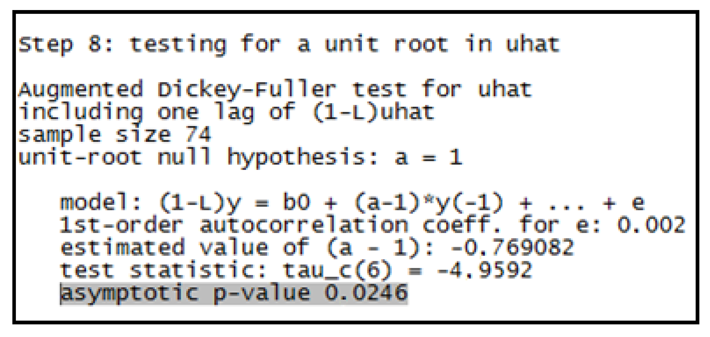
The augmented Dickey–Fuller test was employed to test for cointegration. The testing itself is based on the null hypothesis H₀: the variables are not cointegrated, or the alternative hypothesis H₁: the variables are cointegrated. The subsequent data (Figure 11) are the result of an investigation into the cointegration of the dataset in the Gretl 2025a program.

As illustrated in Figure 11, the p-value is 0.0246. Given that this value is lower than the significance level α = 0.05, it can be concluded that the null hypothesis H₀ must be rejected and the alternative hypothesis H₁ accepted. This indicates that the factors are cointegrated, i.e., they are non-stationary in themselves, but their linear dependencies are stationary. Consequently, spurious regression is not a possibility in mathematical modelling. Similarly, the significantly negative value of tau_c(6) = −4.9592 indicates strong evidence for rejecting the null hypothesis.

The parameters outlined above demonstrate the suitability of the proposed configuration of variables (Table 4). As demonstrated in Equation (23), it is possible to formulate a mathematical model to predict the nitrogen content in desulphurized pig iron (N_DeS). The resulting form of the model is as follows (29):

N_DeS = 0.000105058 + 0.0220528 · A₁ + 2.5678 × 10⁻⁸ · A₂ + 2.50746 × 10⁻⁸ · A₃ − 2.35159 × 10⁻⁶ · A₄ + 4.96884 × 10⁻⁶ · A₅

(29)

where:

N_DeS: predicted nitrogen content in desulphurized pig iron;

A₁: amount of sulfur removed [%];

A₂: amount of blown nitrogen as carrier gas for the desulphurization mixture [l];

A₃: weight of pig iron after desulfurization [kg];

A₄: amount of desulphurization mixture [kg];

A₅: temperature difference of pig iron before and after desulfurization [°C].

• Validity ranges of the model (29) are listed in

  Table 18. Validity range of the N_DeS model (29) for predicting the amount of nitrogen in desulphurized pig iron.

  Parameter	Range of Values
  Amount of sulfur removed [%]	0.017–0.082
  Amount of blown nitrogen as carrier gas for desulphurization mixture [l]	373–14,586
  Weight of pig iron after desulfurization [kg]	139,200–145,500
  Amount of desulphurization mixture [kg]	140–625
  Temperature difference of pig iron before and after desulfurization [°C].	Temp. lowering by 38 °C Temp. increase of 11 °C

  .

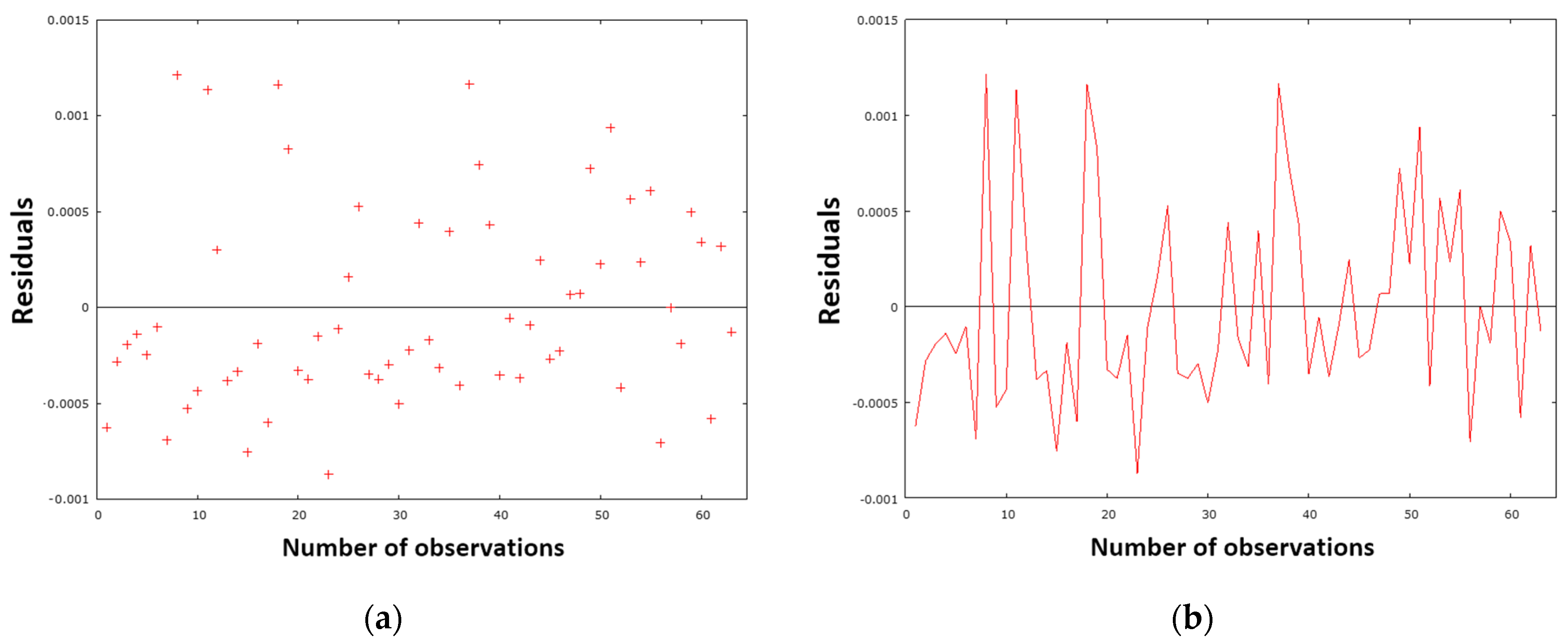
The proposed model was subjected to a rigorous diagnostic process, which involved the utilization of precise testing analyses and graphical tools. This study employed a range of statistical techniques, including tests for normality, heteroscedasticity, multicollinearity, and autocorrelation, to analyze the data. The analysis of the model was facilitated by the utilization of graphical representations, including scatter plots, line graphs, and histograms. The evaluation of the model is based on residuals, which represent the difference between the measured and predicted values of the amount of nitrogen in the desulphurized pig iron. Figure 12a presents a graphical representation of the residual variance, while Figure 12b provides a residual analysis of the timeline.

As demonstrated in Figure 12a, the residual deviations are randomly dispersed around zero, and no potential trend or pattern can be observed in the graph. Consequently, the model is well designed and meets the assumptions. Figure 12b clearly shows that the sign of the residual values changes sufficiently over time. This finding suggests that the designed model generally does not overestimate or underestimate the calculated nitrogen values in metal when making predictions. 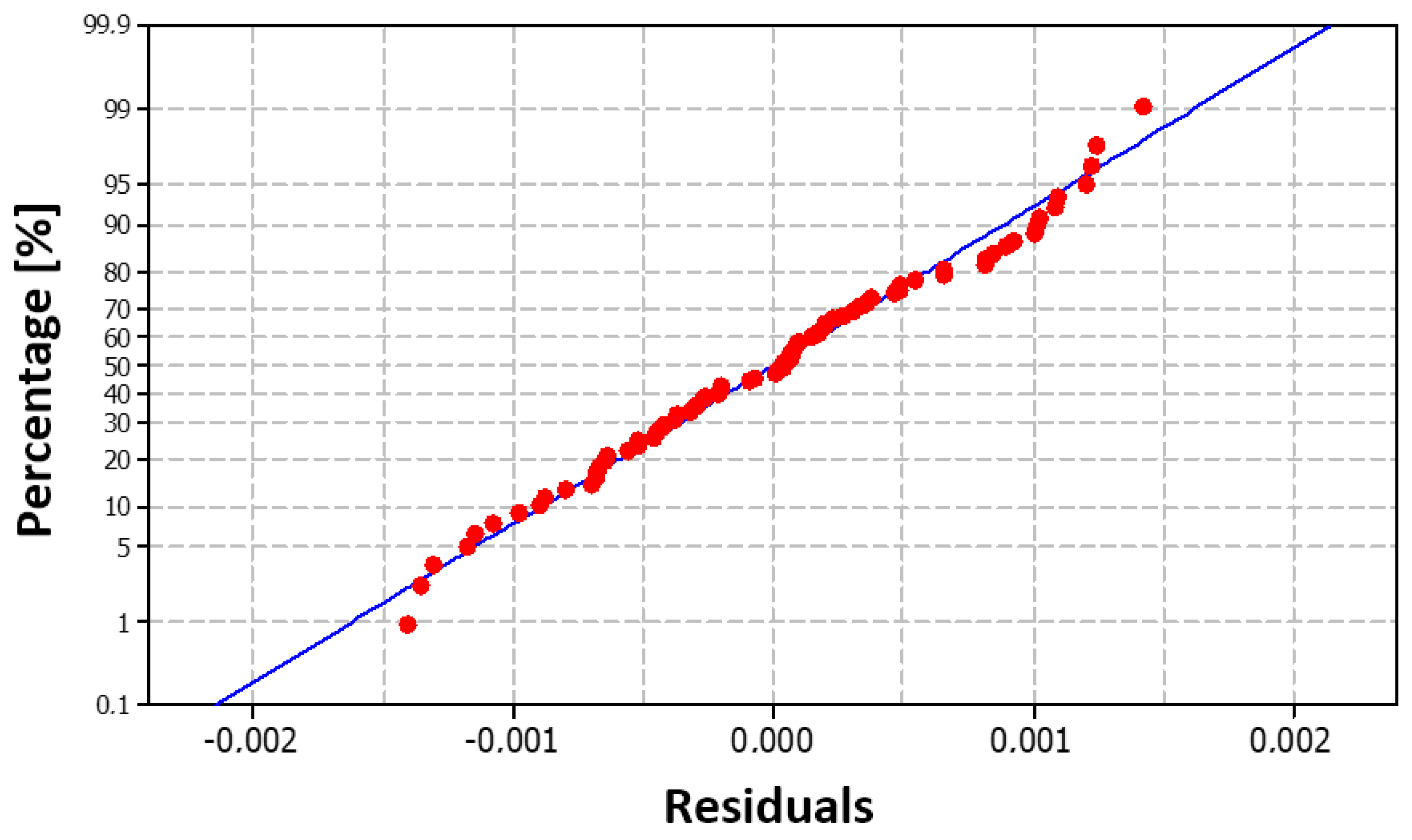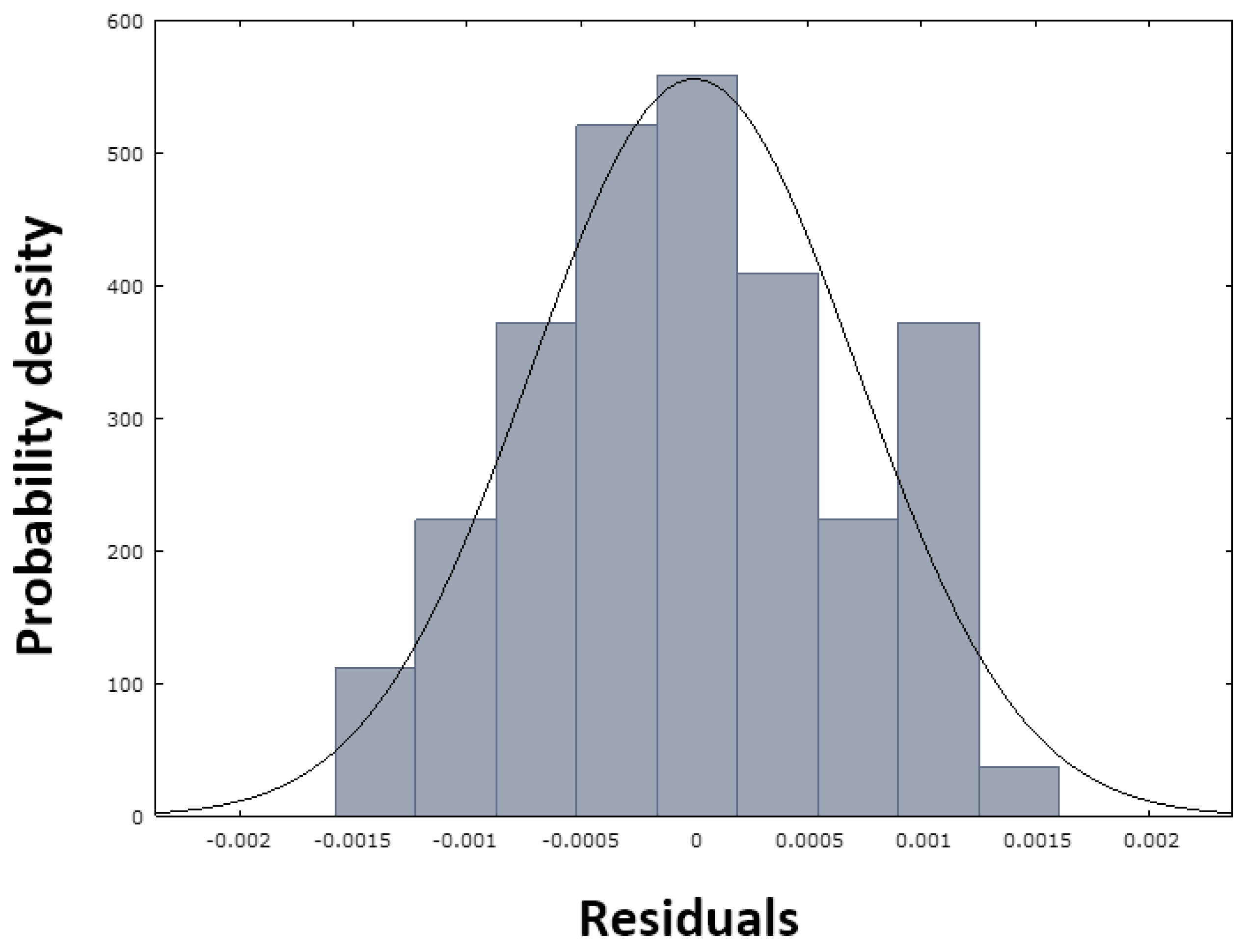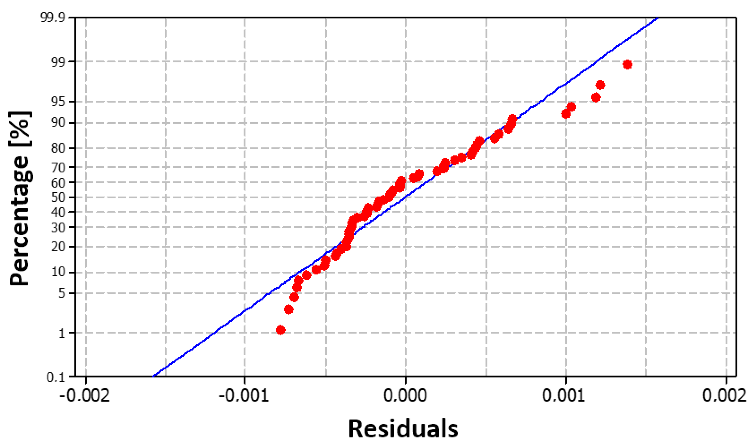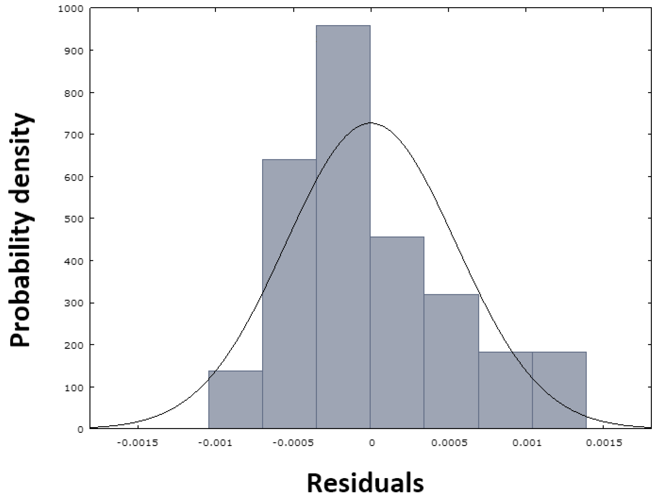The sum of squares of residuals (Table 5) with a value of 0.000036 confirms this opinion, as the value is close to zero. This fact—the normality of the residuals—is also evident from Figure 13, in which the red dots are arranged close to the blue line, demonstrating the normal distribution of the residuals, which is also confirmed by the histogram in Figure 14.

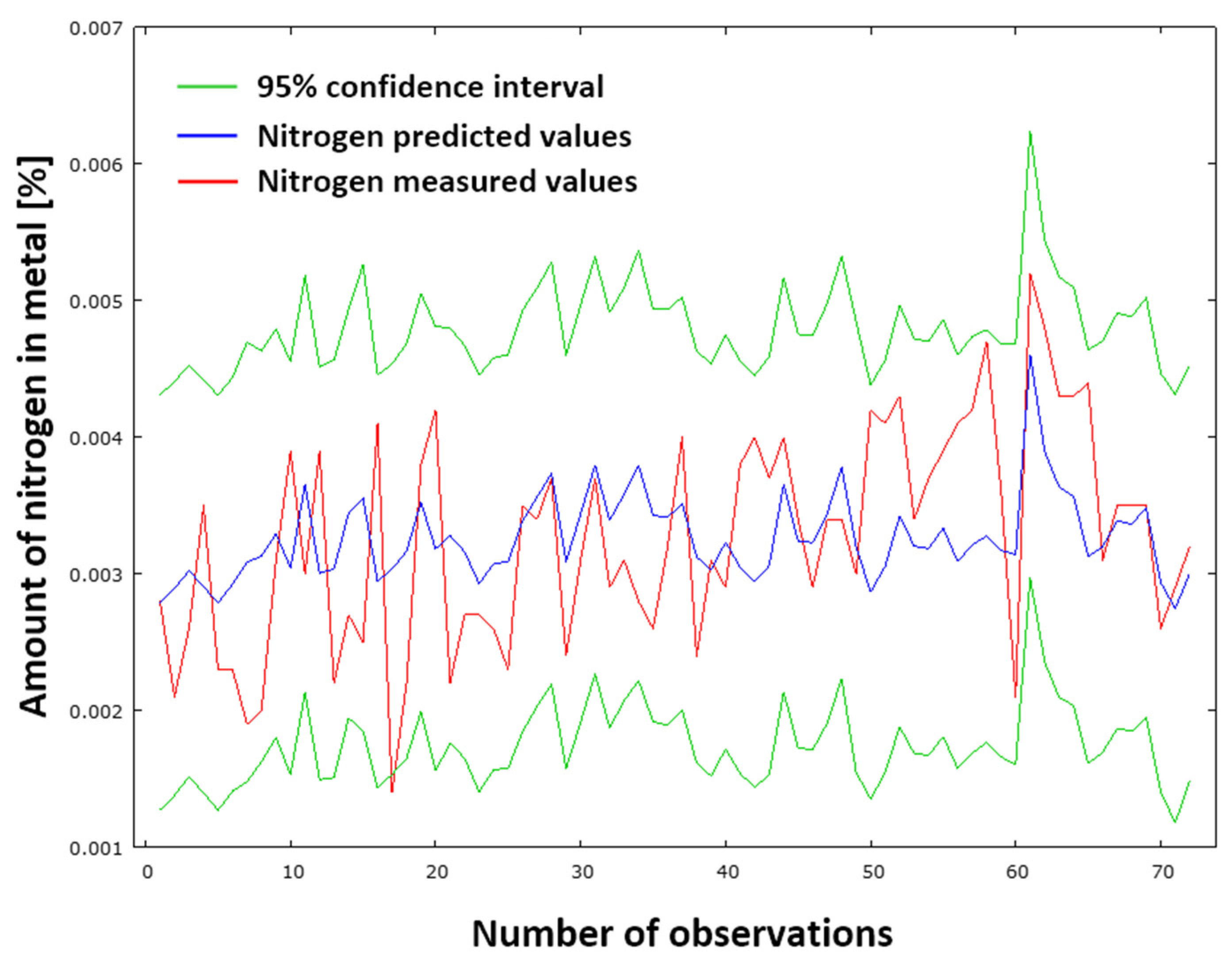
Figure 15 provides a graphical representation of the comparison between measured and predicted results using the N_DeS model (29). The red curve signifies the measured values, whilst the blue curve denotes the predicted values of nitrogen content in pig iron following desulfurization. The green curves represent the 95% confidence interval. The standard deviation of the residuals is 0.000718051. This low value indicates minimal discrepancies between the measured and predicted datasets. Consequently, the N_DeS model (29) provides accurate results.

To detect incorrect specifications in the proposed model, heteroscedasticity tests are used to test the non-constant variance of random components [73]. The tests verify whether any significant variables have been omitted from the mathematical model [74]. White’s heteroscedasticity test and Breusch–Pagan’s heteroscedasticity test were used for testing. For both tests, the null hypothesis H₀ applies: no heteroscedasticity, as opposed to the alternative hypothesis H₁: heteroscedasticity present. The test statistic for White’s test of heteroscedasticity is 15.0079. The null hypothesis is rejected if the value of White’s test statistic is greater than the critical value χ²(20) at the corresponding confidence level α. However, this is not the case, because χ²(20) = 31.41 > 15.0079. Consequently, the null hypothesis H₀ regarding the absence of heteroscedasticity is accepted. The Breusch–Pagan test statistic for heteroscedasticity is 3.00616. The null hypothesis H₀ is rejected if the value of the Breusch–Pagan statistic is greater than the corresponding critical chi-squared value χ²(5) at the chosen confidence level α. However, this is not the case because χ²(5) = 11.07 > 3.00616. Therefore, we accept the null hypothesis (H₀) of the absence of heteroscedasticity. Both tests confirmed the absence of heteroscedasticity, and thus the variance of random components exhibits homoscedasticity, meaning that no significant variable is omitted from the proposed model.

Multicollinearity testing is used to verify the suitability of the factors affecting the amount of nitrogen in metal. In a multiple regression model, multicollinearity assesses the extent to which two or more prognostic factors are correlated. If there is a high degree of correlation, even a small change in the dataset could result in a significant change in the estimated strength of the coefficient. However, multicollinearity does not reduce the model’s overall predictive power and reliability, only affecting the calculations relating to individual predictors [75]. Multicollinearity is assessed by the Variance Inflation Factor (VIF) [76], whose values for the analyzed factors a₁–a₅ (Table 4) are provided in

Table 19. Results of the VIF test for the factors that influence the nitrogen content of desulphurized pig iron.

Parameter	Value
Amount of sulfur removed	3.184
Amount of blown nitrogen as carrier gas for desulphurization mixture	1.127
Weight of pig iron after desulfurization	1.258
Amount of desulphurization mixture	1.089
Temperature difference of pig iron before and after desulfurization	3.468

. The minimum value is 1, with values above 10 indicating high multicollinearity.

Time series extrapolation produces forecasts based on estimates of the parameters of a specific mathematical model whose quality has been confirmed by various statistical tests. Therefore, it can be expected that the resulting forecasts will not differ greatly from reality. The accuracy of the forecasts is assessed using various average characteristics.

The Mean Absolute Error (MAE) is a measure of the average absolute deviation of actual values from estimated (predicted) values. Following the substitution of the given Equation (24), the resulting statistic is found to be MAE_DeS = 1.3374 × 10⁻¹⁰. Consequently, it can be deduced that the Mean Absolute Error is negligible.

The Mean Percentage Error (MPE) expresses the degree of distortion. After substituting into Equation (25), the result MPE_DeS = −3.5785% was obtained. It can, therefore, be concluded that the proposed model systematically overestimates reality, with the predicted values being, on average, 3.5785% higher than the actual values.

The Mean Absolute Percentage Error (MAPE) is a statistical metric that calculates the average magnitude of forecast errors as a percentage relative to actual values over the entire forecast period. Following the substitution of the observed statistic into Equation (26), the result is MAPE_DeS = 16.5411%.

The accuracy of the N_DeS model (29) is determined through the substitution of the model’s parameters into Equation (27). Subsequently, Equation (30) can be established, thereby determining the accuracy of the N_DeS model, as outlined in Equation (31).

$$\mathrm{Model}\mathrm{accuracy}:{\mathrm{N}}_{\mathrm{DeS}}=100-{\mathrm{MAPE}}_{\mathrm{DeS}}$$

(30)

Model accuracy: N_DeS = 83.4589%

(31)

4.2. Model for Predicting Nitrogen Content in Molten Crude Steel Before Tapping from BOF

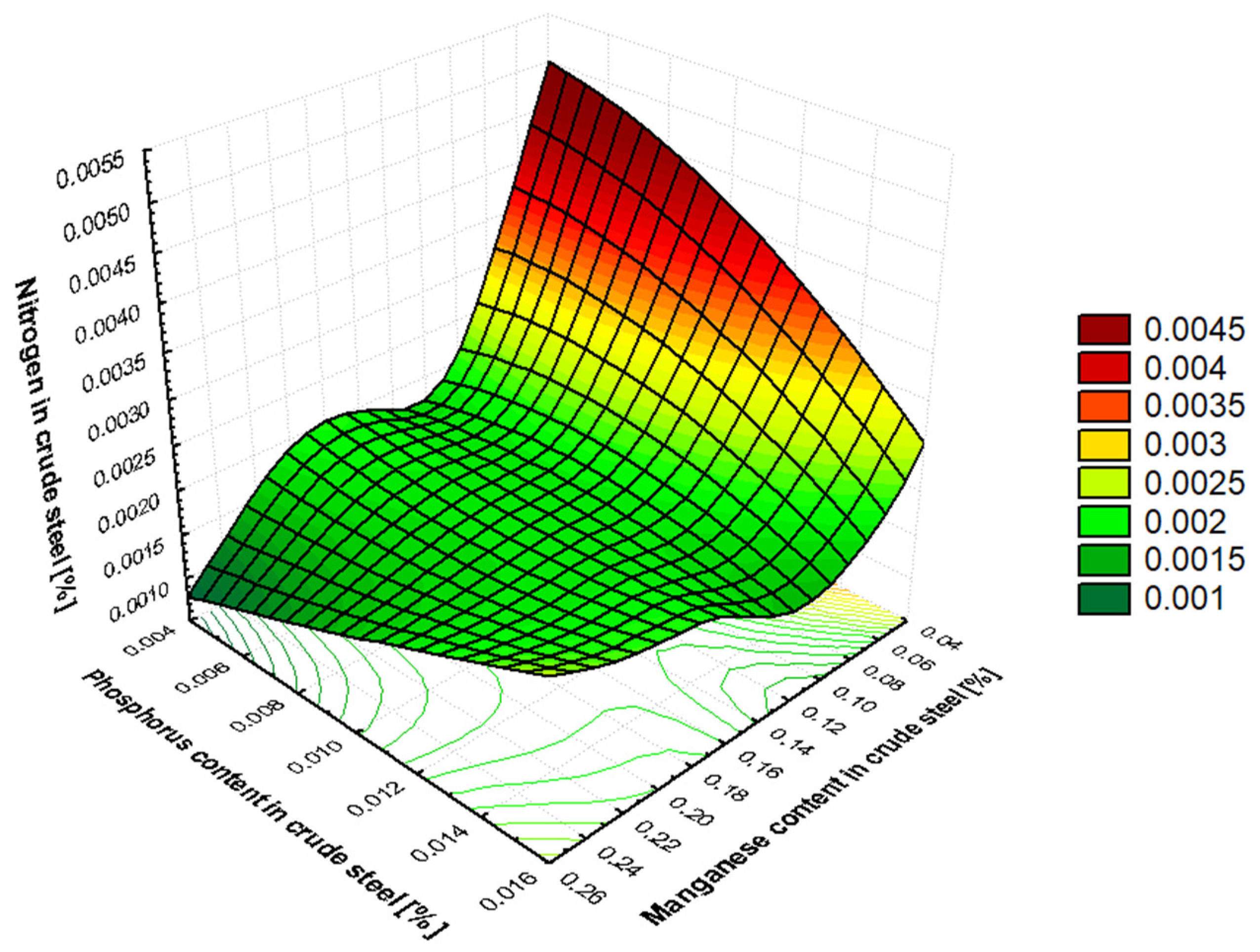
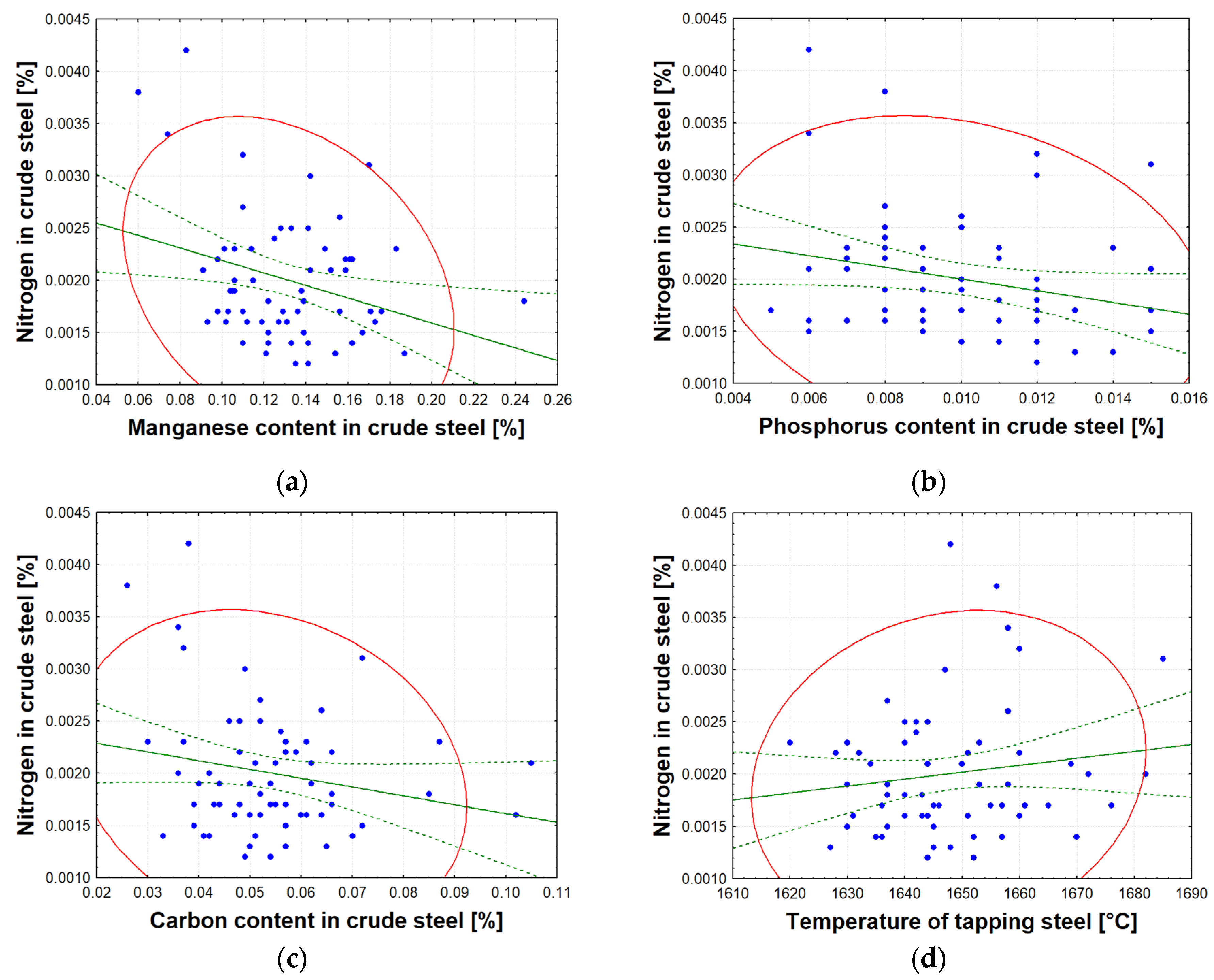
Section 3.2 and Table 6 show the ranking of factors affecting the amount of dissolved nitrogen in crude steel before it is tapped from the BOF. The results can be interpreted as follows: The most significant factor causing increased nitrogen content in crude steel is the total oxygen reblow time, which correlates very well with operational reality. The nitrogen content of high-purity oxygen (oxygen purity level of 95%) can vary significantly, from 70 to 1250 ppm of nitrogen. Reblow is performed either due to an inadequate chemical composition or a low temperature of the crude steel, and this increases the amount of nitrogen dissolved in the metal. The content of manganese, phosphorus, and carbon relates to the amount removed during the refining process. The greater the removal of these elements during heat, the greater the nitrogen content of the crude steel, which is closely related to the blowing time, amount of high-purity oxygen supplied, and intensity of oxygen blowing. The effect of the amount of briquettes added on the increase in dissolved nitrogen in the produced crude steel is related to its binder, molasses. Molasses is used in the production of briquettes at a proportion of up to 10 wt.%. Sugar beet molasses contains nitrogen in its structure and has the chemical formula C₆H₁₂NNaO₃S [77]. Tapping temperature affects the amount of nitrogen dissolved in crude steel. More nitrogen is dissolved at higher tapping temperatures. This is because the solubility of nitrogen in molten steel increases with temperature.

Based on Table 9, it can be observed that correct results were achieved using the OLS method. The standard deviation of the dependent variable (0.000614) when compared to the mean value of the dependent variable (0.002002) yielded a coefficient of variation of approximately 0.31 (SD/Mean). This indicates that the variability of the dependent variable is to a considerable extent governed, and it is estimated to account for approximately 31% of its mean value.

As demonstrated in Table 1, the coefficient of determination, according to Cohen’s distribution, manifests only moderate values. However, it is imperative to underscore the non-stationary nature of data from integrated systems and the fact that these are operational data, for which achieving average correlation coefficients is a substantial accomplishment.

The sum of squares of residuals is 0.000017. A low value indicates that the absolute errors of the model are very small, which is a positive sign for the accuracy of predictions.

The F-test tests whether the null hypothesis H₀ primarily applies, i.e., ${\sigma }_2^2={\sigma }_1^2$, or if the alternative hypothesis applies, i.e., H₁: ${\sigma }_2^2\ne {\sigma }_1^2$. The critical value of the F-distribution for a significance level of 10% is F_crit(7, 55) = 1.829. Since F_crit(7, 55) < F(7, 55), i.e., 1.829 < 2.326593, it can be concluded that the null hypothesis can be rejected, meaning that the standard deviations of the datasets are 90% different from each other.

The Durbin–Watson statistic value of 2.000830 is almost ideal. A value close to 2.0 indicates the absence of autocorrelation in the model residuals, thus supporting the null hypothesis H₀ concerning the absence of autocorrelation. This is a highly positive finding, as it fulfils one of the fundamental assumptions of linear regression, namely, the independence of errors. In Granger–Newbold’s comparison of spurious regression, it is possible to conclude, on the basis of Equation (28), that, in this case, there is no indication of spurious regression, because the value of the coefficient of determination R² is lower than the value of the DW test.

The augmented Dickey–Fuller test was applied to assess cointegration. This test evaluates the null hypothesis, H₀: the variables are not cointegrated, against the alternative hypothesis, H₁: the variables are cointegrated. Figure 16 presents the results of this cointegration analysis, carried out using the statistical tool Gretl 2025a.

As depicted in Figure 16, the p-value is 0.01596, which is below the significance level (α = 0.05), leading us to reject the null hypothesis (H₀) in favor of the alternative (H₁). Consequently, the series are cointegrated: each is non-stationary on its own, but their linear combination is stationary. Accordingly, spurious regression cannot occur in the mathematical model. Moreover, the markedly negative value of tau_c(8) = −5.61958 offers strong evidence for rejecting the null hypothesis.

The test parameters demonstrate the suitability of the configuration of variables listed in Table 8. Equation (23) can be used to create a mathematical model for predicting the nitrogen content of raw steel before tapping it from the basic oxygen furnace. The resulting model takes the form of Equation (32).

N_BOF = −0.0137962 + 7.06124 × 10⁻⁶ · B₁ − 0.000306035 · B₂ − 0.0469186 · B₃ − 0.00499063 · B₄ − 3.44051 × 10⁻⁸ · B₅ + 1.04457 × 10⁻⁵ · B₆ − 3.96352 × 10⁻⁷ · B₇

(32)

where:

N_BOF: predicted nitrogen content in crude steel before tapping from BOF;

B₁: oxygen reblow time [s];

B₂: manganese content in crude steel [%];

B₃: phosphorus content in crude steel [%];

B₄: carbon content in crude steel [%];

B₅: briquettes [kg];

B₆: temperature of tapping steel [°C];

B₇: oxygen blowing time [s].

• The validity ranges of the model (32) are exhibited in

  Table 20. Validity range of the N_BOF model (32) for predicting the amount of nitrogen content in crude steel prior to tapping from BOF.

  Parameter	Range of Values
  Oxygen reblow time [s]	0–100
  Manganese content in crude steel [%]	0.060–0.244
  Phosphorus content in crude steel [%]	0.005–0.015
  Carbon content in crude steel [%]	0.026–0.105
  Briquettes [kg]	0–3260
  Temperature of tapping steel [°C]	1620–1685
  Oxygen flowing time [s]	1601–2322

  .

The proposed N_BOF model (32) followed the same rigorous diagnostic process as the N_DeS model (29). This process involved the use of precise testing analyses and graphical representations. The evaluation of the model is grounded in the assessment of residuals. Residuals serve to illustrate the discrepancy between the measured value and the predicted value of the amount of nitrogen in the crude steel prior to tapping. As illustrated in Figure 17a, the residual variance is presented graphically, while Figure 17b offers a residual analysis with respect to the timeline.

As illustrated in Figure 17a, the residual deviations are randomly dispersed around zero. Furthermore, the graph does not exhibit any discernible trend or pattern. Consequently, the model is well designed and meets the assumptions. As demonstrated in Figure 17b, the sign of the residual values undergoes a substantial alteration over the course of the experiment. This finding suggests that the designed model generally does not significantly overestimate or underestimate the calculated nitrogen values in metal when making predictions. The calculation of the sum of squares of residuals (Table 9) yields a value of 0.000017, which corroborates this viewpoint, as it is proximate to zero. This finding—that is, the normality of the residuals—can be seen in Figure 18, where the points (red dots) can be seen to be arranged quite close to the blue line. This arrangement demonstrates a normal distribution of the residuals. This finding is also confirmed by the histogram in Figure 19.

As illustrated in Figure 20, a graphical representation is provided of the comparison between measured and predicted results using the N_BOF model (32). The red curve represents the measured values, whilst the blue curve denotes the predicted values of nitrogen content in crude steel prior to tapping. The green curves represent the 95% confidence interval. The standard deviation of the residuals is calculated to be 0.000548932. The observed value, which is of negligible magnitude, signifies that there is minimal discrepancy between the two datasets, i.e., the measured and predicted ones, respectively. Consequently, it can be posited that the N_BOF model (32) provides accurate results.

The White and Breusch–Pagan tests were used to assess the presence of heteroscedasticity, and to verify the null hypothesis (H₀), which assumes the absence of heteroscedasticity, and the alternative hypothesis (H₁), which assumes its presence. The White test yielded a value of 34.3269. The null hypothesis is rejected if the value of the test statistic is greater than the corresponding critical value, χ²(34), at the chosen confidence level, α. However, this is not the case because χ²(34) = 48.602 > 34.3269. Therefore, in White’s test, the null hypothesis of no heteroscedasticity is accepted. The Breusch–Pagan test statistic for heteroscedasticity is 8.66205. The null hypothesis (H₀) is rejected if the value of the Breusch–Pagan test statistic is greater than the corresponding critical χ²(7) value at the chosen confidence level α. However, this is also not the case here, as χ²(7) = 14.067 > 8.66205. According to the Breusch–Pagan statistic, the null hypothesis (H₀): no heteroscedasticity is accepted.

As part of the solution to multicollinearity, the variance inflation factor (VIF) is evaluated. The values for the analyzed factors b₁–b₇ (Table 8) are shown in

Table 21. Results of the VIF test for the factors that influence the nitrogen content of crude steel prior to tapping.

Parameter	Value
Oxygen reblow time	1.166
Manganese content in crude steel	2.609
Phosphorus content in crude steel	2.540
Carbon content in crude steel	1.582
Briquettes	1.184
Temperature of tapping steel	1.550
Oxygen flowing time	1.075

. The test results indicate low to no multicollinearity (1 is the minimal value). This indicates that the independent variables are well separated, meaning that each variable contributes unique information to the model. Based on the VIF test, the proposed N_BOF (32) model also shows stability, with reliable regression coefficients that are unaffected by excessive correlation between variables.

The accuracy of the N_BOF model (32) can be evaluated as follows. The Mean Absolute Error (MAE) was calculated using Equation (24), and the result is MAE_BOF = 1.3606 × 10⁻¹⁰. It can therefore be concluded that the average absolute error is very small.

The Mean Percentage Error (MPE) was computed based on Equation (25), and, after substituting into the relationship, the result is MPE_BOF = −6.1515%. It can therefore be concluded that reality is systematically overestimated by the proposed model, with the predicted values being 6.1515% higher than the actual values on average.

The average size of forecast errors compared to actual values across the entire forecast period is expressed using the Mean Absolute Percentage Error (MAPE). Substituting into Equation (26), we obtain the result MAPE_BOF = 22.7696%. The accuracy of the N_BOF model (32) can be determined by substituting the model’s parameters into Equation (27). This establishes Equation (33), which determines the accuracy of the NBOF model as outlined in Equation (34).

$$\mathrm{Model}\mathrm{accuracy}:N_{BOF}=100-MAP{E}_{BOF}$$

(33)

Model accuracy: N_BOF = 77.2304%

(34)

4.3. Model for Predicting Nitrogen Content in Molten Steel at the Beginning of Secondary Metallurgy

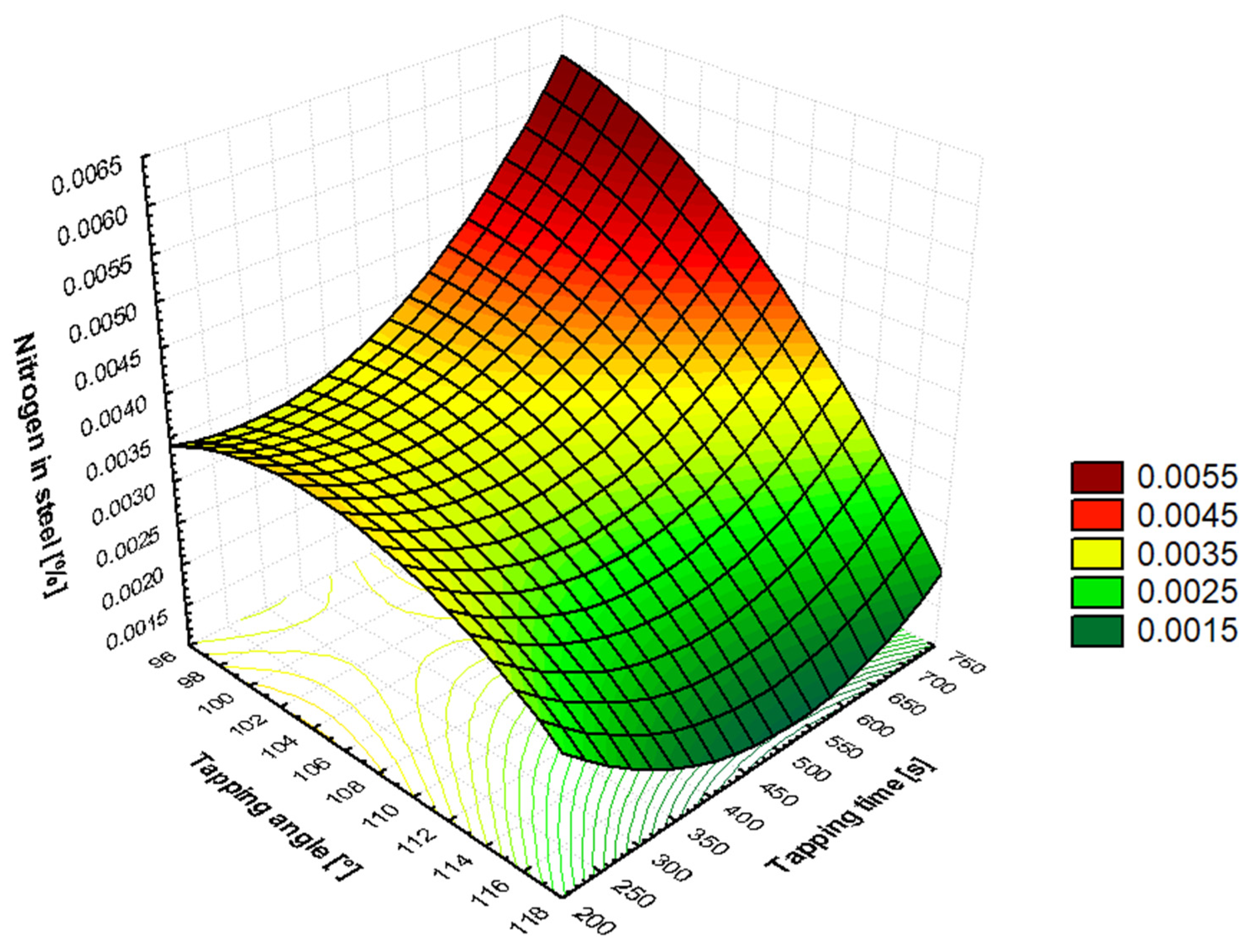
It has been shown in Section 3.3 (Table 10) that, as the tapping angle is increased, the nitrogen content in molten steel is reduced. This dependency is associated with the length of the tapping steel stream. With a smaller BOF vessel tilt, the length of the tapped steel stream is greater, meaning more tapped steel comes into contact with the atmosphere, creating a larger reaction area. As the converter tilt increases, the steel flowing into the ladle is straighter and shorter, resulting in a smaller reaction surface. The duration of the tapping time is also found to be significantly related to the length of time the steel is in contact with air (79% of air consists of nitrogen). It has been demonstrated that an increase in the duration of the tapping time results in an increase in the nitrogen content dissolved in the steel, due to the prolongation of the steel’s exposure to the air. At the beginning of secondary metallurgy, silicon in steel comes from the FeSi ferroalloy. This ferroalloy is added to steel only after a carbonized deoxidizer or carburizing coke is added. This ensures the boiling of the steel and the generation of a large amount of CO bubbles, which subsequently generate CO₂. This reduces the amount of active oxygen at the metal–gas interface, enabling the metal to become supersaturated with atmospheric nitrogen during intense steel boiling. 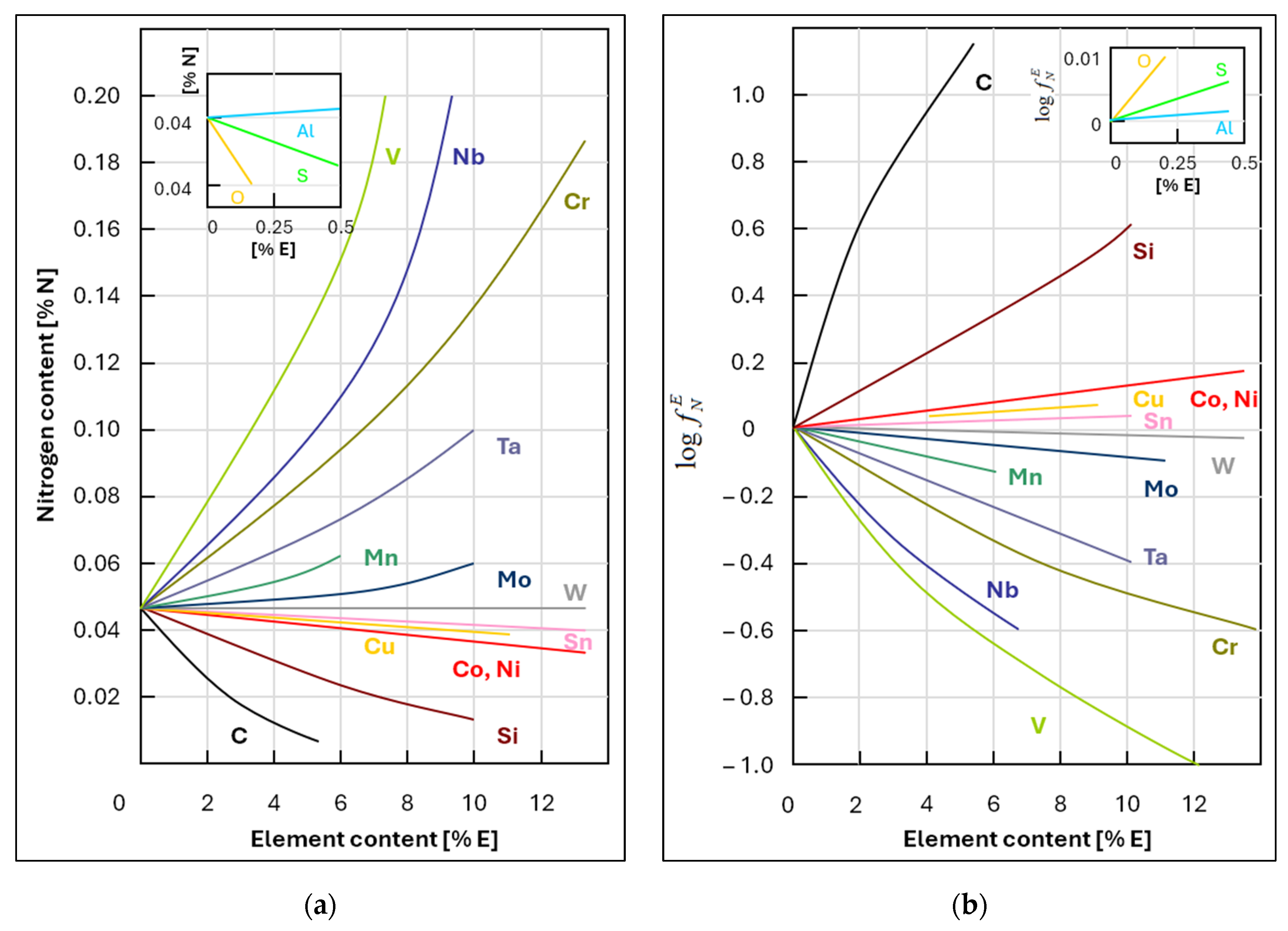After FeSi is added, the silicon also reacts with the active oxygen in the metal to form SiO₂, which increases the nitrogen transfer coefficient into the metal. Depending on the manufacturer, FeSi contains approximately 80–150 ppm of nitrogen. Moreover, Wagner’s interaction coefficient for the Fe–Si–N system is $e_{Si}^N= 0.047$. A positive value indicates that silicon increases the activity coefficient of nitrogen and thus also the equilibrium solubility of nitrogen in molten steel. At the beginning of secondary metallurgy (SM), manganese comes from both the crude steel produced in the BOF and the FeMn aff. alloy added during the SM process. Manganese increases the solubility of nitrogen in steel. Similarly, the FeMn aff. ferroalloy contains 40–80 ppm of nitrogen, depending on the supplier. Wagner’s interaction coefficient for the Fe–Mn–N system is $e_{Mn}^N= 0.013$. 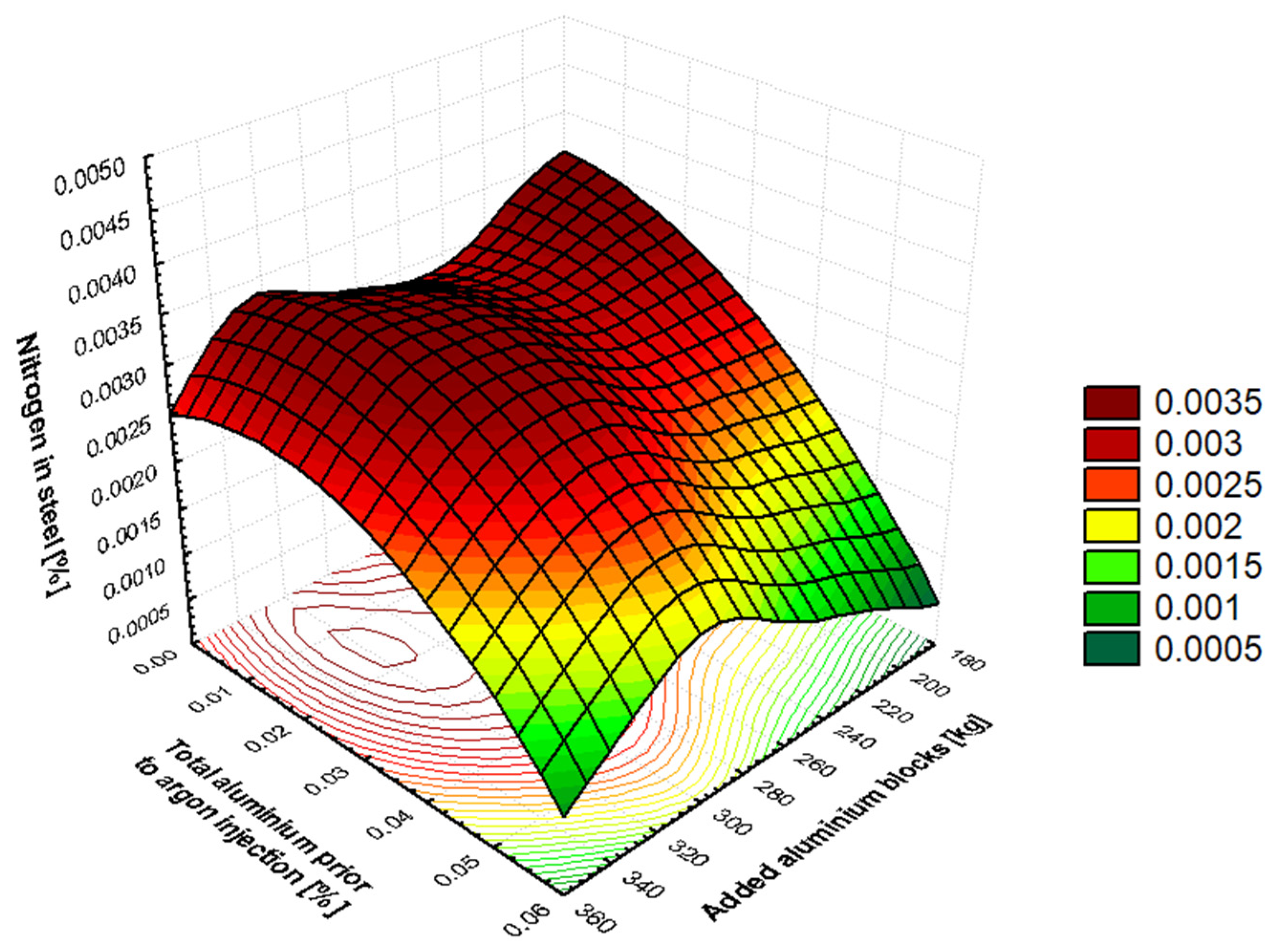A positive value indicates that manganese increases the activity coefficient of nitrogen and thus also the equilibrium solubility of nitrogen in molten steel. Oxygen is a highly active element on the surface of metal and occupies active sites at the metal–gas phase interface. Therefore, oxygen in crude steel slows down the dissolution of nitrogen in the metal. Adding a large amount of aluminum in the form of blocks significantly reduces the activity of oxygen in the metal. This reduces the amount of oxygen at the metal–gas interface and increases the nitrogen transfer coefficient, allowing nitrogen to dissolve into the metal and increasing its content. This is the reason why fully-killed steels have a higher nitrogen content than semi-killed steels, as deoxidation removes more oxygen and requires more added aluminum as a deoxidizer. During this process, the metal is mixed intensively and comes into contact with air. This is why the nitrogen that enters the metal during aluminum-based deoxidation comes from the atmosphere. For steel grades that require a very low final nitrogen value, deoxidation using aluminum is performed during processing at SM with chopped aluminum wire rather than aluminum blocks during tapping from BOF. The efficiency of deoxidation using chopped aluminum wire is 85–92%. Wagner’s interaction coefficient for the Fe–Al–N system is $e_{Al}^N= -0.017$. A negative value indicates that aluminium decreases the activity coefficient of nitrogen, thereby reducing the equilibrium solubility of nitrogen in molten steel. Therefore, adding 0.03% aluminium to the metal reduces the equilibrium nitrogen content by approximately 3–4 ppm at 1600 °C.

The results presented in Table 13 confirm the validity of the ordinary least squares (OLS) estimation approach. The coefficient of variation, calculated as the ratio of the standard deviation (0.000888) to the mean value (0.003160) of the dependent variable, equals approximately 0.28 (SD/Mean). This indicates that the dispersion of the dependent variable is substantially controlled, with the variability representing approximately 28% of the mean value.

As shown in Table 1, according to Cohen’s distribution, the coefficient of determination only exhibits moderate values. However, it is important to emphasize the non-stationary nature of the data from integrated systems, and the fact that these are operational data for which achieving average correlation coefficients is a significant achievement.

The sum of the squares of the residuals is 0.000035. This low value indicates that the model’s absolute errors are very small, suggesting that predictions will be accurate.

The F-test determines whether the null hypothesis (H₀: ${\sigma }_2^2={\sigma }_1^2$) or the alternative hypothesis (H₁: ${\sigma }_2^2\ne {\sigma }_1^2$) applies. The critical value of the F-distribution for a 10% significance level is F_crit(7, 67) = 1.808. As F_crit(7, 67) < F(7, 67), i.e., 1.808 < 6.453, the null hypothesis can be rejected. This means that the standard deviations of the datasets are 90% different from each other.

The Durbin–Watson statistic of 1.872243 (Table 13) provides evidence for the absence of autocorrelation among model residuals, thereby supporting the null hypothesis H₀ regarding the independence of error terms. This finding is particularly significant as it satisfies a fundamental assumption underlying linear regression analysis, specifically the requirement for error independence. According to the Granger–Newbold criterion in Equation (28), no spurious regression is detected since R² < DW, confirming model validity.

The augmented Dickey–Fuller test was employed to examine cointegration relationships among the variables. The test framework evaluates the null hypothesis H₀ (absence of cointegration) against the alternative hypothesis H₁ (presence of cointegration). The cointegration analysis results, conducted using the statistical software Gretl 2025a, are presented in Figure 21.

As illustrated in Figure 21, the p-value is 0.003933, which is significantly below the significance level (α = 0.05). This indicates that the null hypothesis (H₀) is rejected and the alternative (H₁) is accepted. Consequently, the series are cointegrated: each is non-stationary on its own, but their linear combination is stationary and spurious regression is precluded in the mathematical model. Furthermore, the markedly negative value of tau_c(8) = −6.0245 provides substantial evidence to support the rejection of the null hypothesis—series are cointegrated.

The test parameters demonstrate the suitability of the configuration of variables listed in Table 10. Equation (23) can be utilized to formulate a mathematical model for predicting the nitrogen content in steel at the beginning of secondary metallurgy. The resulting model assumes Equation (35).

N_SMB = 0.00982567 − 7.89409 × 10⁻⁵ · C₁ + 0.00368566 · C₂ − 0.00987549 · C₃ + 0.00442257 · C₄ − 0.00140863 · C₅ + 6.15271 × 10⁻⁷ · C₆ + 6.28702 × 10⁻⁶ · C₇

(35)

where:

N_SMB: predicted nitrogen content in steel at the beginning of secondary metallurgy,

C₁: tapping angle [°];

C₂: silicon in molten steel prior to argon bubbling [%];

C₃: total aluminum prior to argon bubbling [%];

C₄: carbon in molten steel prior to argon bubbling [%];

C₅: manganese in molten steel prior to argon bubbling [%];

C₆: tapping time [s];

C₇: added aluminum blocks [kg].

• The validity ranges of the model (35) are illustrated in

  Table 22. Validity range of the N_SMB model (35) for predicting the amount of nitrogen content in steel at the beginning of secondary metallurgy.

  Parameter	Range of Values
  Tapping angle [°]	98–117
  Silicon in molten steel prior to argon bubbling [%]	0–0.403
  Total aluminum prior to argon bubbling [%]	0.006–0.056
  Carbon in molten steel prior to argon bubbling [%]	0.026–0.171
  Manganese in molten steel prior to argon bubbling [%]	0.174–1.290
  Tapping time [s]	249–683
  Added aluminum blocks [kg]	200–350

  .

The proposed N_SMB model (35) was subjected to the same rigorous diagnostic process as the N_DeS model (29) and N_BOF model (32). This process involved precise testing, analysis, and graphical interpretation. The model’s evaluation is based on the analysis of residuals. Residuals illustrate the discrepancy between the measured and predicted amounts of nitrogen in the crude steel prior to tapping. Figure 22a illustrates the residual variance graphically, while Figure 22b provides a residual analysis over time.

As depicted in Figure 22a, the residual deviations exhibit a random distribution around zero without any observable systematic trend or pattern. This distribution confirms that the model is appropriately specified and satisfies the underlying statistical assumptions. As shown in Figure 22b, the sign of the residual values changes substantially over the course of the experiment. This suggests that the designed model generally does not significantly overestimate or underestimate the calculated nitrogen values in metal when making predictions. Calculating the sum of squares of residuals (Table 13) yields a value of 0.000035, which corroborates this viewpoint as it is close to zero. Figure 23 illustrates this finding, showing that the points (red dots) are arranged quite close to the blue line, indicating the normality of the residuals. This demonstrates a normal distribution of the residuals. The histogram in Figure 24 also confirms this finding.

Figure 25 presents a comparative analysis of measured versus predicted values generated by the N_SMB model (35). The graphical representation displays measured values (red curve), predicted nitrogen concentrations in crude steel prior to tapping (blue curve), and the 95% confidence interval (green curves). The calculated standard deviation of residuals is 0.000721066, indicating minimal discrepancy between observed and predicted datasets. This negligible deviation demonstrates that the N_SMB model (35) exhibits satisfactory predictive accuracy.

The White and Breusch–Pagan tests were employed to evaluate the presence of heteroscedasticity and to verify the null hypothesis (H₀), which assumes the absence of heteroscedasticity, and the alternative hypothesis (H₁), which assumes its presence. The White test yielded a value of 42.766. The null hypothesis is to be rejected if the value of the test statistic is greater than the corresponding critical value, χ²(35), at the chosen confidence level, α = 0.05. However, this is not the case, because χ²(35) = 49,802 > 42,766. Consequently, in White’s test, the null hypothesis of no heteroscedasticity is accepted. The Breusch–Pagan test statistic for heteroscedasticity is 4.94841. The null hypothesis (H₀) is rejected if the value of the Breusch–Pagan test statistic is greater than the corresponding critical χ²(7) value at the chosen confidence level. However, this is not applicable in this instance, as χ²(7) = 14.067 > 4.94841. It is evident that, in accordance with the Breusch–Pagan statistic, the null hypothesis (H₀) is accepted, namely that there is no heteroscedasticity.

As part of the solution to multicollinearity, the variance inflation factor (VIF) is evaluated. The values for the analyzed factors c₁–c₇ (Table 12) are shown in

Table 23. Results of the VIF test for the factors that influence the nitrogen content in steel at the beginning of the secondary steelmaking.

Parameter	Value
Tapping angle	1.102
Silicon in molten steel prior to argon bubbling	4.056
Total aluminum prior to argon bubbling	1.133
Carbon in molten steel prior to argon bubbling	6.466
Manganese in molten steel prior to argon bubbling	6.760
Tapping time	1.289
Added aluminum blocks	1.211

. The VIF values indicate that the regression model is relatively favorable. Those that do not exhibit multicollinearity have values close to the ideal of 1, while variables such as carbon, manganese, and silicon in steel exhibit slight multicollinearity but do not exceed the critical VIF value of 10. The VIF values for carbon, manganese, and silicon indicate their correlated behavior. However, their higher VIF test values are not a shortcoming of the model but rather reflect actual metallurgical relationships. This correlation stems from their shared roles in steelmaking processes as they naturally form part of the chemical composition of both raw iron and steel. Due to their similar affinity for oxygen at high temperatures, they react similarly with oxygen, are subject to similar thermodynamic laws in steel production and processing, and influence each other’s final properties. In the context of steel finishing in secondary metallurgy, this correlation is both expected and technologically justified, confirming the accuracy of the statistical analysis observations. Intensive mixing of the steel during tapping from the Basic Oxygen Furnace (BOF), the boiling of the steel at the bottom of the ladle, and the addition of aluminum to deoxidize the steel significantly reduce the amount of nitrogen dissolved in the metal by transporting nitrogen to the metal–slag interface. In secondary steel metallurgy, the correlation between carbon, manganese, and silicon dissolved in steel is a natural phenomenon with fundamental practical significance. Understanding and utilizing this correlation enables more efficient process control, improves product quality in terms of nitrogen content, and generates economic savings. For modern steel producers, this correlation is an invaluable tool for optimizing production processes and ensuring consistent steel quality. Due to this, each variable provides unique information to the N_SMB model (35).

The accuracy of the N_SMB model can be evaluated as follows: The Mean Absolute Error (MAE) was calculated using Equation (24), giving a result of MAE_SMB = 2.407 × 10⁻¹¹. Therefore, it can be concluded that the average absolute error is very negligible.

The mean percentage error (MPE) was computed based on Equation (25). After substituting this into the relationship, the result is MPE_SMB = −5.3582%. Therefore, it can be concluded that the proposed model systematically overestimates reality, with the predicted values being, on average, 5.3582% higher than the actual values.

The Mean Absolute Percentage Error (MAPE) is used to express the average size of forecast errors compared to actual values across the entire forecast period. Substituting this into Equation (26) gives MAPE_SMB = 20.0341%. The accuracy of the N_SMB model can be determined by substituting its parameters into Equation (27). This establishes Equation (36), which determines the accuracy of the NBOF model, as outlined in Equation (37).

$$\mathrm{Model}\mathrm{accuracy}:N_{SMB}=100-MAP{E}_{SMB}$$

(36)

Model accuracy: N_SMB = 79.9659%

(37)

4.4. Model for Predicting Nitrogen Content in Molten Steel at the End of Secondary Metallurgy

The most significant factors affecting the amount of nitrogen dissolved in molten steel (see Table 14) can be described as follows: The solubility of nitrogen in liquid steel is governed by Sievert’s law, whereby the equilibrium solubility of nitrogen in steel increases with temperature. Despite thermodynamics predicting higher nitrogen solubility at higher temperatures, industrial observations demonstrate a contrary trend, whereby the ultimate nitrogen content in steel decreases with increasing temperature during secondary metallurgy. This phenomenon can be attributed to the predominance of kinetic factors over thermodynamic equilibrium. At the beginning of the SM process, a significant number of CO bubbles are generated in the ladle, thereby assisting in the mixing of the melt. It has been demonstrated that at elevated temperatures, there is an increase in the volume of CO bubbles, and that the reaction [C] + [O] = {CO} proceeds at a faster rate [78]. However, at this stage, the elevated presence of surface–active elements, such as oxygen and sulfur, inhibits the process of rapid desulfurization. In the later stages of SM, when the generation of CO is reduced due to the depletion of reagents in the metal, argon assumes the role of the mixing agent. However, it has been demonstrated that, at elevated temperatures, the inhibitory effect of surface–active elements is reduced [79]. It has been demonstrated that, by reducing the amount of oxygen in the metal, it is possible to effectively remove nitrogen from the metal using the residual amount of CO bubbles in combination with argon [80]. The argon is fed into the metal through a porous plug located at the bottom of the casting ladle. As the temperature of the metal is increased, the viscosity of the steel is also reduced, thus facilitating the movement of CO and Ar bubbles. Experimental evidence has demonstrated that elevating the temperature from 1550 °C to 1620 °C enhances the saturation solubility of nitrogen, whereas concurrently increasing the rate constant for nitrogen removal and the mass transfer coefficient has also been observed [81]. During the process of deoxidation of steel tapped from BOF, a carbonized deoxidizer or carburizing coke is added. This process ensures that the steel boils and a large number of CO bubbles are generated. Subsequently, CO₂ is created. This reduces the amount of active oxygen at the metal–gas interface, enabling the metal to become supersaturated with atmospheric nitrogen during intense steel boiling. Adding FeMn aff. (not nitrogenous FeMnN) increases the nitrogen content of steel. The nitrogen in FeMn comes from atmospheric nitrogen that comes into contact with molten FeMn during the production process. Carousel tapping of FeMn creates a large reaction surface between the ferroalloy and the atmosphere, causing the absorption of large amounts of atmospheric nitrogen into the FeMn. The ferroalloy FeMn aff. has been found to contain nitrogen at concentrations ranging from 40 to 80 ppm, with variations depending on the supplier. The interaction coefficient for the Fe–Mn–N system, as determined by Wagner, is $e_{Mn}^N= 0.013$. A positive value indicates that manganese increases the activity coefficient of nitrogen, thus increasing the equilibrium solubility of nitrogen in molten steel. The final manganese content at the end of secondary metallurgy is closely related to the amount of FeMn added during the secondary metallurgy stage of steel processing.

The results presented in Table 17 confirm the validity of the ordinary least squares (OLS) estimation approach. The coefficient of variation, calculated as the ratio of the standard deviation (0.000790) to the mean value (0.003270) of the dependent variable, equals approximately 0.24 (SD/Mean). Consequently, the dataset displays low relative dispersion, indicating that variability constitutes only 24% of the central tendency. This supports the ordinary least squares assumptions, thereby confirming the methodological soundness of the OLS estimator and validating the reliability of the inferences derived from Table 17.

In the context of analyzing industrial data from steel production, the value of R² = 0.241736 can be considered acceptable. Industrial processes are characterized by high variability and complex interactions between process variables. Consequently, even a low value of R² can be informative and useful, especially if the regression coefficients are statistically significant and the result of the coefficient of determination can, therefore, be considered significant in terms of the nature of the data being processed.

The sum of the squares of the residuals is 0.000033. It is evident that the low value indicates that the model’s absolute errors are minimal, thereby suggesting that predictions will be accurate.

The F-test is a statistical procedure used to determine whether the null hypothesis (H₀: ${\sigma }_2^2={\sigma }_1^2$) or the alternative hypothesis (H₁: ${\sigma }_2^2\ne {\sigma }_1^2$) applies. The critical value of the F-distribution for a 10% significance level is F_crit(4, 67) = 2.031. As F_crit(4, 67) < F(4, 67), i.e., 2.031 < 2.682089, the null hypothesis can be rejected. This indicates that the standard deviations of the datasets differ by 90%.

With a value of 2.029951, the Durbin–Watson statistic is almost ideal. A value close to 2.0 indicates an absence of autocorrelation in the model residuals, thus supporting the null hypothesis (H₀) of an absence of autocorrelation. This is a highly positive finding as it fulfils one of the fundamental assumptions of linear regression: the independence of errors. According to Granger and Newbold’s comparison of spurious regression, the relation in Equation (28) suggests that there is no indication of spurious regression in this case, as the value of the coefficient of determination R² is lower than the DW test value.

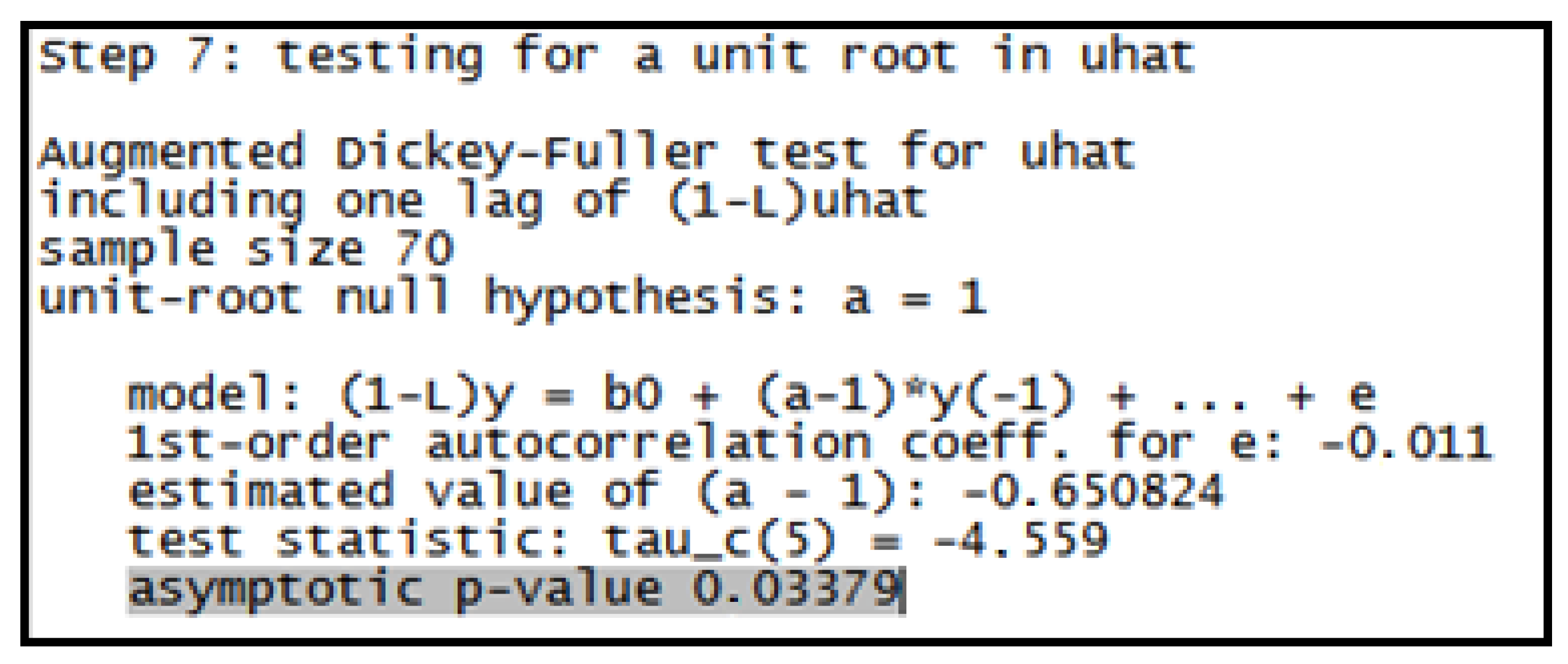
The augmented Dickey–Fuller test was used to analyze the cointegration relationships between the variables. This test evaluates the null hypothesis (H₀: absence of cointegration) against the alternative hypothesis (H₁: presence of cointegration). The results of the cointegration analysis, which was conducted using the Gretl 2025a statistical software, are presented in Figure 26.

As shown in Figure 26, the p-value is 0.03379, which is below the significance level α = 0.05. This indicates that the null hypothesis (H₀) is rejected, and the alternative hypothesis (H₁) is accepted. Consequently, the series are cointegrated: while each series is non-stationary on its own, their linear combination is stationary. Therefore, spurious regression can be ruled out in the mathematical model. Furthermore, the markedly negative value of tau_c(5) = −4.559 provides substantial evidence in support of rejecting the null hypothesis. For this reason, the series are cointegrated.

The test parameters demonstrate the suitability of the configuration of variables listed in Table 14. Equation (23) can be employed to formulate a mathematical model for predicting the nitrogen content in steel at the conclusion of secondary metallurgy. The resulting model assumes the form of Equation (38).

N_SME = 0.0257714 − 1.45992 × 10⁻⁵ · D₁ + 0.0126950 · D₂ + 3.08438 × 10⁻⁶ · D₃ − 0.00153525 · D₄

(38)

where:

N_SME: predicted nitrogen content in steel at the end of secondary metallurgy;

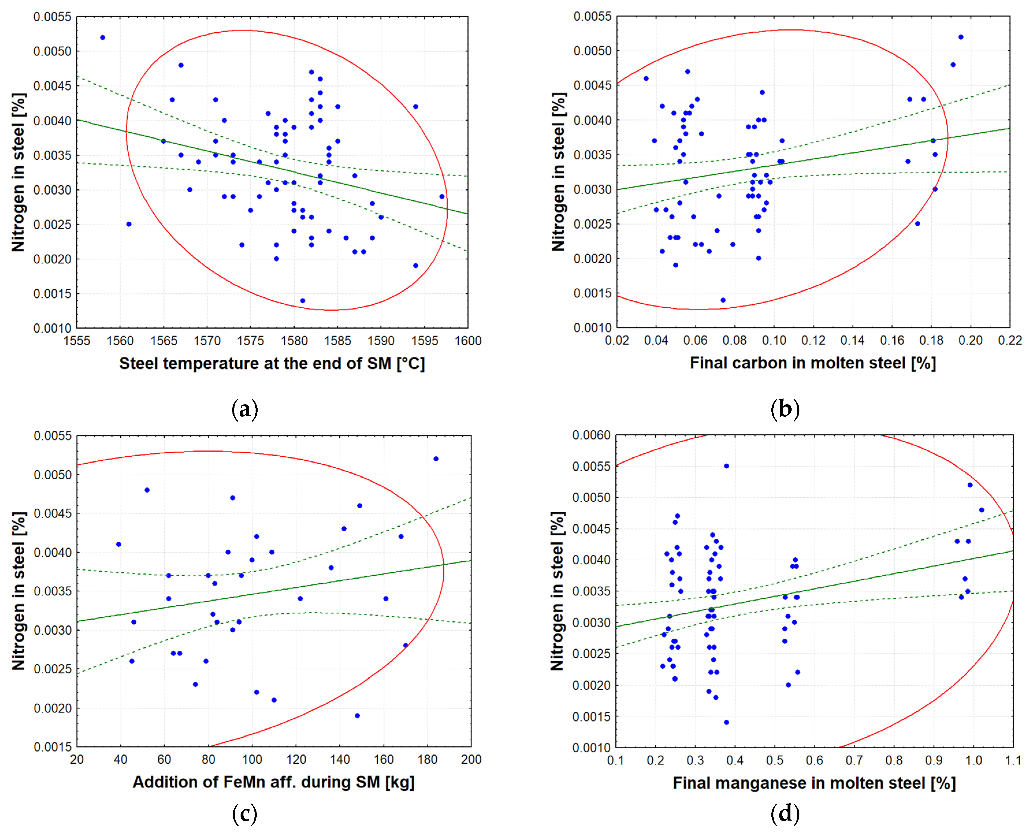
D₁: steel temperature at the end of SM [°C];

D₂: final carbon in molten steel [%];

D₃: addition of FeMn aff. during SM [%];

D₄: final manganese in molten steel [%].

• The validity ranges of the model (38) are illustrated in

  Table 24. Validity range of the N_SME model (38) for predicting the amount of nitrogen content in steel at the end of secondary metallurgy.

  Parameter	Range of Values
  Steel temperature at the end of SM [°C]	1558–1597
  Final carbon in molten steel [%]	0.039–0.195
  Addition of FeMn aff. during SM [%]	0–184
  Final manganese in molten steel [%]	0.218–1.380

  .

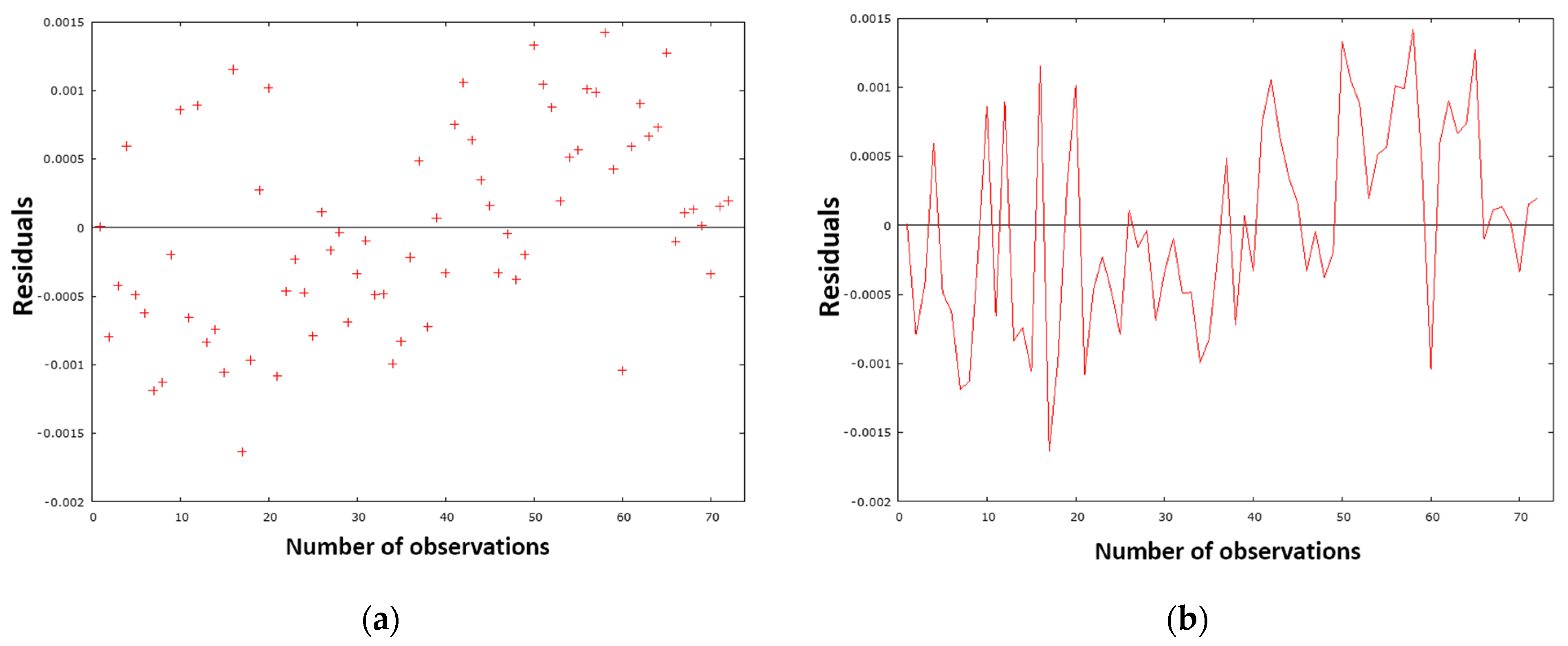
The proposed N_SME model (38) was subjected to the same rigorous diagnostic process as previous models. The process entailed methodical testing, thorough analysis, and graphical interpretation. The evaluation of the model is based on an analysis of residuals. As illustrated in Figure 27a, the residual variance is presented graphically, while Figure 27b provides a residual analysis over time.

The distribution of residuals in Figure 27a suggests that the random homoscedasticity assumption is valid, which is favorable for the model’s reliability. However, the time series in Figure 27b reveals potential issues of serial correlation and systematic sampling (around observations 15–20), though testing for autocorrelation of residuals does not confirm these. It can therefore be concluded that the model is adequately specified.

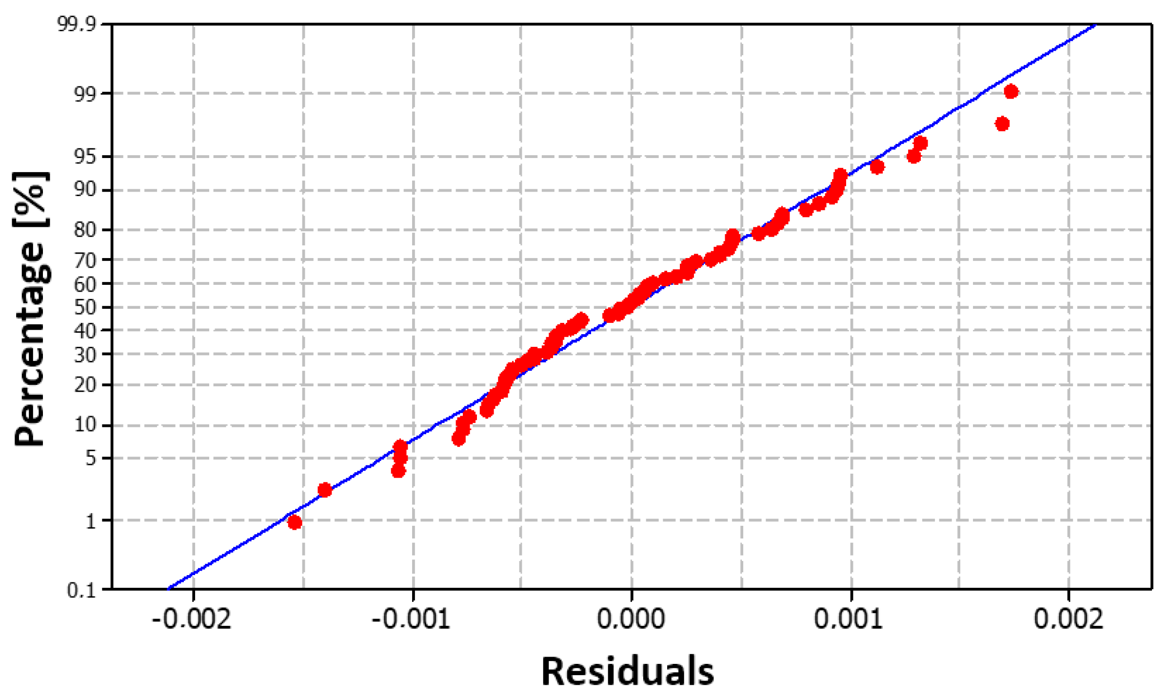
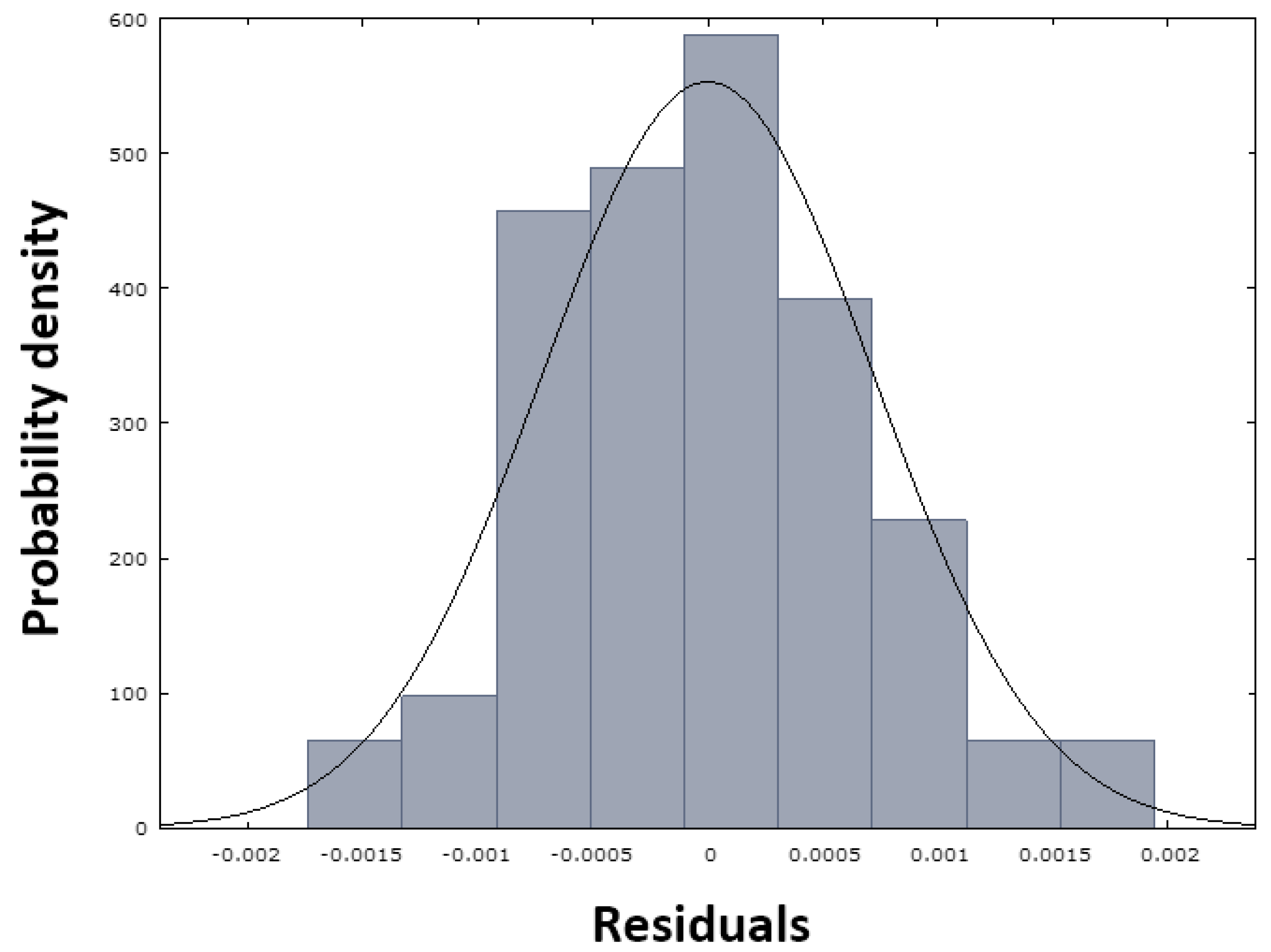
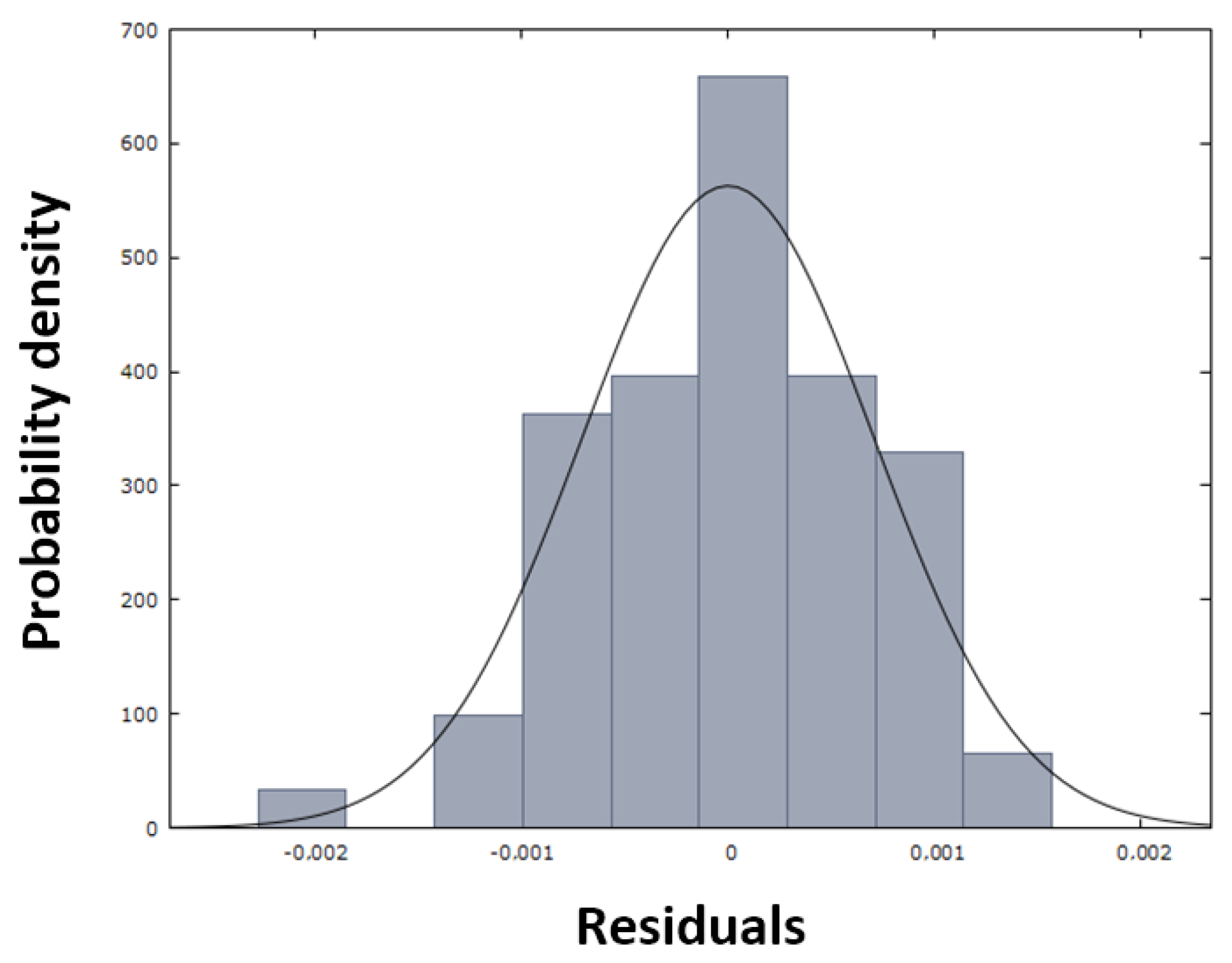
Both diagnostic plots (Figure 28 and Figure 29) suggest that the residuals exhibit an approximately normal distribution, with slight deviations from perfect normality, particularly at extreme values and at the peak of the distribution. For practical purposes, however, we can consider the assumption of residual normality to be sufficiently satisfied.

Figure 30 shows a comparison of the measured and predicted values generated by the N_SME model (38). The graph shows the measured values (red curve), the predicted nitrogen concentrations in crude steel prior to tapping (blue curve), and the 95% confidence interval (green curves). The calculated standard deviation of residuals is 0.00070872, indicating a minimal discrepancy between the observed and predicted datasets. This negligible deviation shows that the N_SME model (38) has satisfactory predictive accuracy.

The White and Breusch–Pagan tests were employed to evaluate the presence of heteroscedasticity and to verify the null hypothesis (H₀), which assumes the absence of heteroscedasticity, and the alternative hypothesis (H₁), which assumes its presence. The White test yielded a value of 15.7133. The null hypothesis is to be rejected if the value of the test statistic is greater than the corresponding critical value, χ²(14), at the chosen confidence level, α = 0.05. However, this would not be the case because χ²(14) = 23.685 > 15.7133. Due to this, in White’s test, the null hypothesis of no heteroscedasticity is accepted. The Breusch–Pagan test statistic for heteroscedasticity is 3.90746. The null hypothesis (H₀) is rejected if the value of the Breusch–Pagan test statistic is greater than the corresponding critical χ²(4) value at the chosen confidence level. However, this is not applicable in this instance, as χ²(4) = 9.488 > 3.90746. It is evident that, in accordance with the Breusch–Pagan statistic, the null hypothesis (H₀) is accepted, namely, that there is no heteroscedasticity.

The variance inflation factor (VIF) is evaluated as part of the solution to multicollinearity. The VIF values for the analyzed factors d₁–d₄ (Table 16) are shown in

Table 25. Results of the VIF test for the factors that influence the nitrogen content in steel at the end of the secondary steelmaking.

Parameter	Value
Steel temperature at the end of SM [°C]	1.665
Final carbon in molten steel [%]	6.103
Addition of FeMn aff. during SM [%]	1.009
Final manganese in molten steel [%]	5.867

. These values indicate that the regression model is relatively favorable. The resulting VIF statistics indicate either no multicollinearity (values around 1) or slightly increased multicollinearity (values around 6). However, all values are below the critical threshold of 10, indicating that serious multicollinearity problems do not threaten the model. The analysis of VIF values confirms the statistical robustness of the regression model. Higher values for carbon and manganese are technologically justified by the chemical dependence of these elements in steelmaking processes. Therefore, the model can be considered suitable for further analysis without the need to eliminate variables or make further structural adjustments. Because of this, each variable provides unique information to the N_SME model (38).

The accuracy of the N_SMB model can be evaluated as follows: The Mean Absolute Error (MAE) was calculated using Equation (24), giving a result of MAE_SME = 0.00056649. Therefore, it can be concluded that the average absolute error is very small.

The mean percentage error (MPE) was computed based on Equation (25). After substituting this into the relationship, the result is MPE_SME = −5.6189%. Consequently, it can be deduced that the proposed model systematically overestimates reality, with the predicted values being, on average, 5.6189% higher than the actual values.

The Mean Absolute Percentage Error (MAPE) is used to express the average size of forecast errors compared to actual values across the entire forecast period. Substituting into Equation (26) yields MAPE_SME = 19.6271%. The accuracy of the N_SME model can be determined by substituting its parameters into Equation (27). This establishes Equation (39), which determines the accuracy of the N_SME model, as outlined in Equation (40).

$$\mathrm{Model}\mathrm{accuracy}:N_{SME}=100-MAP{E}_{SME}$$

(39)

Model accuracy: N_SME = 80.3729%

(40)

5. Conclusions

The presented research introduces a comprehensive system of predictive models for nitrogen content control in steel across individual production stages in the basic oxygen furnace process. Four specialized mathematical models based on the Ordinary Least Squares (OLS) method were successfully developed, covering key technological stages: pig iron desulfurization (N_DeS), crude steel before tapping from BOF (N_BOF), beginning of secondary metallurgy (N_SMB), and end of secondary metallurgy (N_SME).

The results demonstrate that the proposed models achieve satisfactory predictive accuracy with the following values: N_DeS = 83.46%, N_BOF = 77.23%, N_SMB = 79.97%, and N_SME = 80.37%. A hierarchy of factors influencing nitrogen content was identified for each stage, revealing that the most significant factors vary depending on the technological phase of production.

The acquired values were then subjected to a series of verification methods, including a heteroscedasticity test, a normality test, an autocorrelation test, a collinearity test, and a graphical examination of the distribution of residuals. In order to verify the accuracy of the proposed model using modern regression analysis, econometric cointegration analysis was also applied. All algorithms and methodologies that were subjected to rigorous testing during the steel production and processing phases that were monitored were found to provide conclusions that serve to confirm the proposed models for predicting nitrogen in metal. Consequently, it can be concluded that the results obtained from the proposed prediction formulas are reliable within the calculated accuracy of the model and boundary conditions.

The data being exclusively sourced from U. S. Steel Košice, Slovakia, means that the developed models reflect the unique technological conditions, raw material characteristics, and operational procedures specific to this facility. Through effective knowledge transfer and subsequent integration into process control systems, these models could facilitate initiative-taking parameter optimization while reducing dependence on laboratory testing times, thereby preventing excessive nitrogen content in the final steel products.

The proposed models are designed to serve as a practical tool for predicting nitrogen values in metal at specific production stages. This has the potential to enhance the efficiency of the production process and reduce the costs associated with chemical analysis of metal for the presence of nitrogen. The models created are valid within the specified ranges of values for individual parameters (Table 18, Table 20, Table 22, and Table 24), which also correspond to the prescribed values of the chemical composition of the analyses steel grades, whose chemical composition is given in Section 2. In order to enhance the accuracy and robustness of predictive models, the following recommendations are proposed: the implementation of advanced machine learning algorithms, such as neural networks, random forest, or support vector machines, which have the capacity to better capture nonlinear relationships between variables; and the expansion of the dataset with additional operational parameters and longer time series, in order to increase statistical significance.